Valuing Retail Shopping Center Lease Contracts

Hoon ChoΨ James D. Shilling†

University of Wisconsin University of Wisconsin

April 2006

Abstract

In this paper we set up a simple real option model of retail shopping center leases. Themodel incorporates the effects of stochastic sales externalities and the possibility of tenantdefault. The model sheds new light on a number of puzzles: Why a Jorgensonian usercost of capital may overestimate shopping center values. Why retail tenants pay theirlandlord a percentage of revenue (above a sales breakpoint) in addition to a traditionalfixed rent. Why an increase in sales volatility may reduce, rather than increase, the valueof a shopping center. Why base and percentage rents may move positively together, andnot negatively as others have suggested. Why retail property capitalization rates andinterest rates can be negatively, as opposed to positively, related with each other. And:Why leases with a percentage of sales rental are often given little or no value for purposesof financing by lenders, regardless of whether or not the tenant is a national chain withsubstantial net worth.

Keywords: options, stochastic sales externalities, and retail shopping centers

JEL Classification: G12

ΨUniversity of Wisconsin, School of Business, Madison, Wisconsin 53706, Email: hooncho@students.wisc.edu.

†University of Wisconsin, School of Business, Madison, Wisconsin 53706, Email: jshilling@bus. wisc.edu.

For helpful comments, we thank Martha Peyton and Thomas Park.

1. Introduction

The pricing of retail leases has especially received attention in studies by Benjamin, Boyle and

Sirmans (1990, 1992), Brueckner (1993), Colwell and Nunneke (1998), Pashigian and Gould

(1998), and Gould, Pashigian, and Prendergast (2005), and by Grenadier (1995, 1996), Hen-

dershott and Ward (2000, 2002), Moordian and Yang (2000), Clapham (2003), and Benjamin

and Chinloy (2004). The studies by Benjamin, Boyle and Sirmans (1990, 1992), Brueckner

(1993), Colwell and Nunneke (1998), Pashigian and Gould (1998), and Gould, Pashigian, and

Prendergast (2005) discuss the pricing of retail leases in a deterministic framework in which

consumers are drawn to shop at the center by the reputation and advertising of the major

retailer. These models have problems, however, in valuing percentage of sales rentals, rent

bumps, expense stops, etc.

The studies by Grenadier (1995, 1996), Hendershott and Ward (2000, 2002), Mooradian

and Yang (2000), Clapham (2003), and Benjamin and Chinloy (2004), on the other hand,

discuss the pricing of retail leases in a framework in which sales follow a stochastic process.

In these models, feedback effects, such as the loss of a major tenant (or a decline in the

tenant’s customer drawing power) on sales, the center’s occupancy rate, and rent levels of the

other tenants, are generally ignored. Therefore, these models systematically underestimate

risk and overestimate value when default is an important element in the analysis.

The present study integrates these two lines of research. The model developed here treats

the stochastic component of store sales in a manner similar to Hendershott and Ward (2000,

2002), and shared and generative business within the shopping center in a manner similar to

Brueckner (1993). Additionally, the model allows for any tenant of any size to default, and

for default of a key anchor tenant under the lease agreement to lead to further defaults by

1

other tenants.

We assume tenants have a claim on all future profits (modeled as a stochastic process)

and the market value of the center represents the expectation of these cash flows discounted

at a constant risk-adjusted discount rate. Tenants are price-takers in the leasing market,

competing with many other tenants in a perfectly competitive market. Rental prices are fixed

for the term of the lease at lease commencement. These rental prices vary by type of tenant

so as to take into account customer-drawing ability. The single optimization problem is for

the tenant to determine when to exercise his or her default option.

The solution to the model follows by applying stochastic dynamic programming. The

analysis is performed on a lease by lease basis. The results are summed across all leases to

obtain the market value of the center. Different sets of simulation are then carried out to

examine the comparative statics of the model and study the impact of shifts in rental rates

and the level of return on valuation.

Several new results emerge. One, the usual certainty theory for measuring the user cost

of a retail lease as the sum of the expected risk-adjusted discount rate, plus the depreciation

incurred and minus the rate of asset price change no longer applies. The user cost also needs to

include a risk premium to compensate the owner/tenant for the risk that the sales externality

effects at the center could dissipate or disappear over time. Two, and somewhat related,

ignoring this risk premium may significantly overestimate shopping center value. Three, the

greater the expected volatility in sales, the less valuable is the lease contract to the owner.

Others have suggested that the more uncertain the sales, the greater the value of the shopping

center. Four, base and percentage rents in our model may move positively together, and not

negatively as others have suggested. Five, retail property capitalization rates and interest

2

rates can be negatively, as opposed to positively, related with each other (as we shall show

below). Six, the model reveals a perhaps somewhat latent role for percentage of sales rentals:

namely, to offset the negative value to center owners of the tenant’s option to cease to operate

at the center or, at worst, to default.1

But this is not all. The model also helps to explain why leases with a percentage of sales

rental are often given little or no value for purposes of financing by lenders. If the role of

percentage of sales rentals is, in fact, to offset the negative value to center owners of the

tenant’s option to default, this would mean that percentage rents and tenant defaults would

not have to be taken into account in the valuation, as long as the default-free lease cash flows

were discounted at the risk-adjusted rate of return.

The remainder of the paper is organized as follows. The paper first develops a model

for the pricing of retail leases that depends on thirteen parameters, one of those being the

extent to which individual tenants take advantage of one another as to confer benefits on

one another. The paper then describes the initial parameterization of the model. Next, we

present a discussion of the simulation results, followed then by conclusions.

2. Model Setup

There are n different tenants at the shopping center. Each tenant signs a (long-term) lease

with a fixed base rent, and a percentage rent clause. Tenants let space at the center at time

t = 0 and remain there until default; there are no tenant default costs. This assumes all leases1Compare this to Benjamin, Boyle, and Sirmans (1990), and Brueckner (1993): who argue that percentage

rents serve as a mechanism to shift risk from susceptible tenants to landlords who can better handle risk;however, for this to happen the optimal contract needs to be in the form of a pure percentage rent and cannothave a fixed rent component (see Lee (1995)). Miceli and Sirmans(1995) offer a substantially different account,in which percentage lease agreements are used to coordinate the behaviors of multiple interdependent tenantsthrough a common agent, the shopping center owner. Wheaton (2000), and Riddiough and Williams (2005)argue that percentage lease agreements are used to align the interest of the shopping center owner with thatof the tenants.

3

have a co-tenancy or kick-out clause, which allows tenants at the center to default without

further cost if one of the anchor tenants at the center defaults or ceases to operate, or if sales

should fall below a certain level.2

Formally, we let Si(t) stand for sales per square foot for tenant i. Sales are produced with

the help of two factors, the amount of space that is occupied by tenant i and the amount of

space allocated to the other tenants, according to the constant-elasticity production function

Si(t) = Di(t) ·Xi(t)Qλi

i

∏

j 6=i

Qγji

j . We use Qi and Qj to denote the amount of space occupied

by tenants i and j, respectively. The elasticities of production are λi and γji, where λi < 0

and γji is either negative or positive. For example, a higher Qi(t) means a lower Si(t), and

a higher Qj(t) means a higher Si(t), on condition, obviously, that tenant j confers a positive

externality on tenant i. Should γji = 0, tenant j would confer no externality on tenant

i and, should γji be negative, tenant j would generate a negative externality. We use the

following notation, Xi, to denote demand shocks (i.e., something that causes a shift in the

production function). We assume Xi(t) is an event that evolves as a geometric Brownian

motion, hence dXi(t) = µiXi(t)dt + σiXi(t)dZi(t), where µi is the instantaneous conditional

expected percentage change in Xi per unit time, σi is the instantaneous conditional standard

deviation per unit time, and dZi(t) represents the increments of a standard Weiner process.

We use the notation, Di(t), to account for normal depreciation. We assume that Di(t) follows

the deterministic function dDi(t) = −θiDi(t)dt and Di(0) = 1, where θi is the economic rate

of depreciation applied to Di(t).

In certain parts of the paper (for comparison purposes) we will focus on three different

2The one sure way for sales at the center to fall below a certain level is for one of the anchor tenants todefault (see Gatzlaff, Sirmans, and Diskin (1994)). However, there are many other variables to consider andthis is not the only way that center sales can fall. For example, center sales can fall, and fall hard, if thecenter finds itself being anchored by the number 3, 4, or 5 grocer in the market and losing market share toWal-Mart, or if the center finds itself being anchored by an all-around department store and losing marketshare to “category killers” like Home Depot, Toy-R-Us, or Circuit City.

4

lease contracts: a pure fixed rent contract, a profit share rent contract (where the tenant pays

nothing but percentage rent), and a percentage rent contract (where the tenant pays a base

rent plus an overage rent, giving the center owner higher annual rents in years when tenant

sales are particularly strong). For that purpose, we provide here the definitions of these

(i) a pure fixed rent contract is given by P ai (t) = αi for all sales, where α equals a fixed

base rent.

(ii) a profit share rent contract is given by P bi (t) = αi + βiSi(t), where βi is an overage

rate, and βiSi(t) can be viewed as an incentive payment to the center owner.

(iii) a percentage rent contract is given by P ci (t) = αi +βi[Si(t)− Si] · I [Si(t) > Si], where

Si is a sales threshold level and I [Si(t) > Si] represents an indicator function, 1 if Si(t) > Si

and 0 otherwise.

We assume (for computational simplicity) that all other operating costs (e.g., property charges

such taxed, insurance, and maintenance) are zero.3

The approach in the paper is to perform a lease by lease analysis to estimate the dollar

value of each lease. We then sum across all leases to obtain the market value of the center.

We assume that the center owner is the developer and landlord. We assume that the

center owner has already decided the amount of investment and the optimal tenant mix at

the center. Also, the center owner has decided on αi, βi, Si. We assume that these contract

terms are set in a competitive market. Tenants choose when (and whether at all) to exercise

the option to leave the center.

3These recoveries often have significant value to the center owner, which means that valuations ignoringthese recoveries will be too low.

5

3. Value of a Pure Fixed Rent Contract

We can compute the present value of a pure fixed rent contract as follows. Let Vi(Qi, Q−i, Xi(0),

Di(0)) be tenant i’s profit function (in present value terms). This value function is just the

expected (discounted) value of all future profits, i.e.,

Vi(Qi, Q−i, Xi(0), Di(0)) = E0[

∞∫

0

e−rit(Si(t) − P ai (t)) ·Qi(t))dt] (1)

where Q−i = {Q1, Q2, . . . , Qi−1, Qi+1, . . . , Qn} and ri is a constant risk-adjusted discount

rate – constant because risk is assumed to be unchanging during the life of the lease, and

risk-adjusted because we assume Xi(t) grows at µi rather than at a risk-neutral rate. The

infinite time horizon structure in (1) implies that there need not be a definite date when the

tenant must cease to operate or elect to default.

The problem is to choose a boundary where tenant i is free to terminate its lease (without

further cost) in order to maximize (1). We define the Hamilton-Jacobi-Bellman equation by

riV (Qi, Q−i, Xi, Di) = E[(Si(t) − P ai (t)) ·Qi(t))] +

E[dV ]dt

(2)

That is, the return on investment, riV (Qi, Q−i, Xi, Di), equals the per period cash flow,

E[(Si(t) − P ai (t)) · Qi(t))], plus the expected rate of capital gain, E[dV ]

dt . Then using Ito’s

lemma we can write

E[dV ] = {µiXiVX +12σ2

iX2i VXX − θiDiVD +

∑

j 6=i

pji}dt (3)

where VX is the first derivative of V with respect to Xi, VXX is the second derivative of V

with respect to Xi, VD is the first derivative of V with respect to Di, and pji is given by

6

pji ≈ E

[VQj

dQj

dt

](4)

Here pji represents the expected change in V (Qi, Q−i, Xi, Di) due to the possible exit of

tenant j from the mall (which could occur when tenant j’s retail sales fall below some critical

level). pji has two components: the expected loss if tenant j defaults, VQj , and the probability

that default will occur, dQj

dt .4

The general solution to (3) is

V (Qi,Yi) = A1(Qi)Y θi

i +B1(Qi)Yi + C1(Qi) (5)

where Yi = DiXi. The default boundary condition where tenant i is free to exit the mall

occurs when Y ∗i falls below a certain multiple ki of Qi, where kiQi is an exogenous value, not

controlled by uncertainty. The value of kiQi can be viewed as a certain recovery or liquidation

value – i.e., what the tenant walks away with when he or she leaves the center. One would

expect the value of kiQi to be quite small, since most retailers typically maintain restricted

cash accounts and have few tangible assets. Further, because the focus of the paper is on

what happens when tenant i finds itself in a situation where one of the major tenants at the

center has already gone bankrupt or ceases to operate, or on what happens when the center

is losing market share and sales to other centers, no reletting of Qi is permitted.

The value matching condition at the trigger value of Y ∗i is

V (Qi,Y∗i ) = A1(Qi)Y ∗θi

i +B1(Qi)Y ∗i + C1(Qi) = kiQi (6)

4Reasonable parameter values are: VQj= 0.25 (from Gatzlaff, Sirmans and Diskin (1994), who conclude

that non-anchor tenant rents decline by an estimated 25% after the loss of a major tenant) anddQj

dt= 0.03

to 0.04 (from our simulation analysis). This suggests a value of pji in the 0.0075 to 0.0100 range.

7

This condition is easy to interpret. It equates the value of the default option to the certain

recovery value.

The smooth-pasting condition is

∂F (Qi,Y∗i )

∂Y ∗i

= θiA1(Qi)Y ∗θi−1i +B1(Qi) = 0 (7)

where

θi =−

(µi − θi − 1

2σ2i

)−

√(µi − θi − 1

2σ2i

)2 + 2σ2i (ri + pi)

σ2i

and

pi =∑

j 6=i

pji and pi ≥ 0.

This condition ensures that the function relating the default option to the certain recovery

value at the point of default has zero slope.

The value function that satisfies these two conditions is

V (Qi,Yi) = 11 − θi

(αi

ri + pi+ ki

)Qi

(Yi

Y ∗i

)θi

+

Qλi+1i

∏

j 6=i

Qγji

j

ri + θi − µi + piYi − αiQi

ri + pi

(8)

where

Y ∗i =

θi

θi − 1

(αi

ri + pi+ ki

)ri + θi − µi + pi

Qλi

i

∏

j 6=i

Qγji

j

.

8

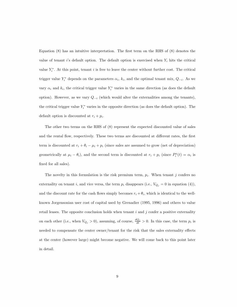
Equation (8) has an intuitive interpretation. The first term on the RHS of (8) denotes the

value of tenant i’s default option. The default option is exercised when Yi hits the critical

value Y ∗i . At this point, tenant i is free to leave the center without further cost. The critical

trigger value Y ∗i depends on the parameters αi, ki, and the optimal tenant mix, Q−i. As we

vary αi and ki, the critical trigger value Y ∗i varies in the same direction (as does the default

option). However, as we vary Q−i (which would alter the externalities among the tenants),

the critical trigger value Y ∗i varies in the opposite direction (as does the default option). The

default option is discounted at ri + pi.

The other two terms on the RHS of (8) represent the expected discounted value of sales

and the rental flow, respectively. These two terms are discounted at different rates, the first

term is discounted at ri + θi − µi + pi (since sales are assumed to grow (net of depreciation)

geometrically at µi − θi), and the second term is discounted at ri + pi (since P ai (t) = αi is

fixed for all sales).

The novelty in this formulation is the risk premium term, pi. When tenant j confers no

externality on tenant i, and vice versa, the term pi disappears (i.e., VQj = 0 in equation (4)),

and the discount rate for the cash flows simply becomes ri + θi, which is identical to the well-

known Jorgensonian user cost of capital used by Grenadier (1995, 1996) and others to value

retail leases. The opposite conclusion holds when tenant i and j confer a positive externality

on each other (i.e., when VQj > 0), assuming, of course, dQj

dt > 0. In this case, the term pi is

needed to compensate the center owner/tenant for the risk that the sales externality effects

at the center (however large) might become negative. We will come back to this point later

in detail.

9

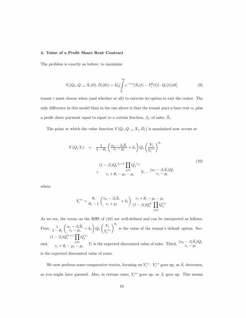
4. Value of a Profit Share Rent Contract

The problem is exactly as before: to maximize

Vi(Qi, Q−i, Xi(0), Di(0)) = E0[

∞∫

0

e−rit(Si(t) − P bi (t)) ·Qi(t))dt] (9)

tenant i must choose when (and whether at all) to exercise its option to exit the center. The

only difference in this model than in the one above is that the tenant pays a base rent αi plus

a profit share payment equal to equal to a certain fraction, βi, of sales, Si.

The point at which the value function V (Qi, Q−i, Xi, Di) is maximized now occurs at

V (Qi,Yi) = 11 − θi

(αi − βiSiri − pi

+ ki

)Qi

(Yi

Y ∗∗i

)θi

+

(1 − βi)Qiλi+1

∏

j 6=i

Qjγji

ri + θi − µi − piYi −

(αi − βiSi)Qiri − pi

(10)

where

Y ∗∗i =

θi

θi − 1

(αi − βiSi

ri + pi+ ki

)ri + θi − µi − pi

(1 − βi)Qλi

i

∏

j 6=i

Qγji

j

As we see, the terms on the RHS of (10) are well-defined and can be interpreted as follows.

First, 11 − θi

(αi − βiSiri − pi

+ ki

)Qi

(Yi

Y ∗∗i

)θi

is the value of the tenant’s default option. Sec-

ond,

(1 − βi)Qλi+1i

∏

j 6=i

Qγji

j

ri + θi − µi − piYi is the expected discounted value of sales. Third, (αi − βiSi)Qi

ri − pi

is the expected discounted value of rents.

We now perform some comparative statics, focusing on Y ∗∗i . Y ∗∗

i goes up, as Si decreases,

as you might have guessed. Also, in certain cases, Y ∗∗i goes up, as βi goes up. This means

10

that tenants are more likely to walk away when they are only getting a limited upside.

Mathematically, these results follow from

∂Y ∗∗i

∂Si= θi

1 − θi· βiri + pi

· ri + ρi − µi + pi

(1 − βi)Qλii

∏

j 6=i

Qγjij

< 0

∂Y ∗∗i

∂βi= θi

1 − θi· Si − αi − (ri + pi)ki

(1 − βi)(ri + pi)· ri + ρi − µi + pi

(1 − βi)Qλii

∏

j 6=i

Qγjij

>< 0

This latter expression is positive if Si ≤ αi + (ri + pi)ki.

5. Value of a Percentage Rent Contract

Now we turn to an analysis of percentage rent contracts. The model in outline form is as

follows. We define Vi(Qi, Q−i, Xi(0), Di(0)) for a percentage rent contract as

Vi(Qi, Q−i, Xi(0), Di(0)) = E0[

∞∫

0

e−rit(Si(t) − P ci (t)) ·Qi(t))dt] (11)

We need to determine two value functions; a value function describing the value of the lease

when Si(t) ≤ Si, which we denote as VA(Qi, Yi), and a value describing the value of the lease

when Si ≥ Si(t), which we denote as VB(Qi, Yi).

These two value functions are given by

VA(Qi, Yi) = A1(Qi)Y ωi1i +A2(Qi)Y ωi2

i +

Qλi+1i

∏

j 6=i

Qγji

j

ri + θi − µi + piYi −

αiQi

ri + pi(12)

and

11

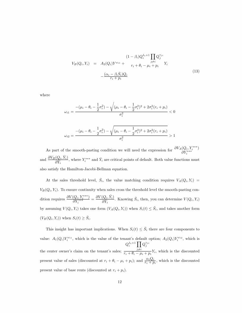
VB(Qi, Yi) = A3(Qi)Y ωi1 +

(1 − βi)Qλi+1i

∏

j 6=i

Qγji

j

ri + θi − µi + piYi

− (αi − βiSi)Qiri + pi

(13)

where

ωi1 =−(µi − θi −

12σ2

i ) −√

(µi − θi −12σ2

i )2 + 2σ2i (ri + pi)

σ2i

< 0

ωi2 =−(µi − θi −

12σ2

i ) −√

(µi − θi −12σ2

i )2 + 2σ2i (ri + pi)

σ2i

> 1

As part of the smooth-pasting condition we will need the expression for ∂VA(Qi, Y∗∗∗i )

∂Y ∗∗∗i

and ∂VB(Qi, Yi)∂Yi

, where Y ∗∗∗i and Yi are critical points of default. Both value functions must

also satisfy the Hamilton-Jacobi-Bellman equation.

At the sales threshold level, Si, the value matching condition requires VA(Qi, Yi) =

VB(Qi, Yi). To ensure continuity when sales cross the threshold level the smooth-pasting con-

dition requires ∂V (Qi, Y∗∗∗i )

∂Y ∗∗∗i

= ∂V (Qi, Yi)∂Yi

. Knowing Si, then, you can determine V (Qi, Yi)

by assuming V (Qi, Yi) takes one form (VA(Qi, Yi)) when Si(t) ≤ Si, and takes another form

(VB(Qi, Yi)) when Si(t) ≥ Si.

This insight has important implications. When Si(t) ≤ Si there are four components to

value: A1(Qi)Y ωi1i , which is the value of the tenant’s default option; A2(Qi)Y ωi2

i , which is

the center owner’s claim on the tenant’s sales;

Qλi+1i

∏

j 6=i

Qγji

j

ri + θi − µi + piYi, which is the discounted

present value of sales (discounted at ri + θi − µi + pi); and αiQiri + pi

, which is the discounted

present value of base rents (discounted at ri + pi).

12

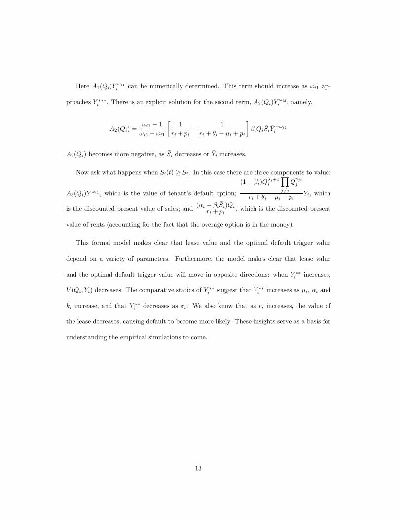
Here A1(Qi)Y ωi1i can be numerically determined. This term should increase as ωi1 ap-

proaches Y ∗∗∗i . There is an explicit solution for the second term, A2(Qi)Y ωi2

i , namely,

A2(Qi) =ωi1 − 1ωi2 − ωi1

[1

ri + pi− 1ri + θi − µi + pi

]βiQiSiY

−ωi2i

A2(Qi) becomes more negative, as Si decreases or Yi increases.

Now ask what happens when Si(t) ≥ Si. In this case there are three components to value:

A3(Qi)Y ωi1 , which is the value of tenant’s default option;

(1 − βi)Qλi+1i

∏

j 6=i

Qγji

j

ri + θi − µi + piYi, which

is the discounted present value of sales; and (αi − βiSi)Qiri + pi

, which is the discounted present

value of rents (accounting for the fact that the overage option is in the money).

This formal model makes clear that lease value and the optimal default trigger value

depend on a variety of parameters. Furthermore, the model makes clear that lease value

and the optimal default trigger value will move in opposite directions: when Y ∗∗i increases,

V (Qi, Yi) decreases. The comparative statics of Y ∗∗i suggest that Y ∗∗

i increases as µi, αi and

ki increase, and that Y ∗∗i decreases as σi. We also know that as ri increases, the value of

the lease decreases, causing default to become more likely. These insights serve as a basis for

understanding the empirical simulations to come.

13

6. Parameterization of the Model

The exogenous variables in the model are the following:

1. tenant mix: Qi and Q−i = {Q1, Q2, . . . , Qi−1, Qi+1, . . . , Qn}

2. production and sales externality parameters: λi and γji for each tenant

3. demand shock parameters: µi and σi

4. rate of economic depreciation: θi

5. lease contract terms: αi, βi, and Si

6. initial sales level: Si(0)

7. discount rate and risk premium: ri and pi

8. liquidation value: ki

A study of retail leases might take several forms, including the pricing of leases used in

community, neighborhood, regional, superregional, fashion/specialty, power, theme/festival,

outlet, and lifestyle centers. This paper studies one of these forms viz. neighborhood centers.

We take a representative neighborhood center from a large institutional real estate owner

and investor. The center has 34 tenants. The tenant mix is: 2 anchor tenants and 32 non-

anchors (see below). We parameterize our model to match this center’s lease terms and sales

information. This adds a degree of realism to the analysis.

The parameter µi is set equal to 3%; our best guess on the nominal growth in retail sales.

θi is of no real import because µi − θi is what matters in the model; so a set of µ and θ’s can

be selected to be consistent with any value of V . We set θi = 0.

The discount rate ri and risk premium pi are set to match the survey data reported in

Korpacz, a quarterly survey of real estate investors concerning office, retail, apartment, and

industrial returns. We set ri = 8% and pi = 1%, for an overall (unlevered) required return

of 9%. (As an aside, Shilling (2003) notes that there seems to be a significant equity risk

14

premium puzzle in real estate. Here the inclusion of the term pi helps to explain why this

premium might exist, at least for retail properties, that is.) We set the valuation multiple

ki = 2. This valuation multiple is consistent with those derived from market transactions as

reported by Kozloff (2005).

The remaining parameter values – Qi and Q−i = {Q1, Q2, . . . , Qi−1, Qi+1, . . . , Qn}, λi

and γji, α, βi, and S, and Si(0) – are discussed in more detail in the next two sections.

7. Estimating the Stochastic Sales Externalities among Retail Tenants

7.1 Estimation Model

This section deals with the estimation of the stochastic sales externalities (ρji) between ten-

ants. Assume that retailers fall into two categories, anchor and nonanchor tenants. A linear

time trend specification for identifying the stochastic component of sales (per square foot) for

retailers that are anchor tenants is

ln(Sj(t)/Qj) = a0f1 + a1f2 + a2t+ a3W + εaj (t) j = 1, 2 (14)

and that for nonanchor tenants is

ln(Si(t)/Qi) = b0x1 + b1x2 + b2x3 + b4t+ b5ln(Qi) + b6W + εbi (t) i = 1, . . . , 32 (15)

where f1 and f2 are fixed effects dummies (that take the value 1 for anchor tenant j and 0

otherwise), x1, x2, and x3 are tenant size dummy variables equal to 1 when Qi for tenant i

is below 2000 square feet, between 2000 and 4000 square feet, and above 4000 square feet,

respectively, t is a time trend (ranging from 1 in September 2003 to 25 in September 2005), W

15

is a seasonal dummy variable, which takes a value of 1 in December (since sales in December

are significantly higher than other months) and 0 otherwise, and εaj (t) for j = 1, 2 and εbi (t) for

i = 1, 2, . . . , 32 are i.i.d. error terms, where εaj (t) ∼ N(0, σ2(εaj (t))) and εbi (t) ∼ N(0, σ2(εbi (t))),

respectively.

Our first test is to test if equation (14) applies to both anchor tenants j = 1, 2, or whether

two different models should be used. For this test, we will construct a Chow test. We first

estimate (14) separately, once using only the data for anchor tenant j = 1 and the other for

using the data for anchor tenant j = 2. We then pool our data into one set and estimate

equation (14) for both j = 1, 2. A Chow test fails to indicate any difference in the two

equations. The computed F-value is only 1.12, falling below the level of significance for

rejection (p-value = 0.30).

Our second test is to test if equation (15) applies to all 32 nonanchor tenants, or whether

separate models should be used. Here we run a Chow test with 32 equations. The estimated

F-value is 1.18, which fails to reject the null hypothesis that the slope and intercept parameters

are distinct (p-value = 0.31).

We use equation (14) to estimate the residuals εa1(t) and εa2(t) for anchor tenants j = 1, 2 for

each period t. We use equation (15) to estimate an average residual εb(t) across all nonanchor

tenants i = 1, 2, . . . , 32 for each period t. We then regress εb(t) on εa1(t) and εa2(t). That is,

we estimate

εb(t) = τ0εa1(t) + τ1ε

a2(t) + ζ(t) (16)

where τ0 =√ρ1σ(εb(t))σ(εa1(t))

, τ1 =√ρ2σ(εb(t))σ(εa2(t))

, ζ(t) =√

1 − ρ1 − ρ2σ(εb(t))σ(ζ(t)) ψ(t), ρ1 = Corr(εb(t),

16

εa1(t)), ρ2 = Corr(εb(t), εa2(t)), and ψ(t) is an error term. This equation follows from the de-

finition of Corr(εb(t), εai (t)) for i = 1, 2. From (14) and (15), we can obtain estimates for

σ(εa1(t)), σ(εa2(t)), and σ(εb(t)). From (16), we can obtain an estimate of σ(ψ(t)). This allows

us to solve for ρ1 and ρ2 (the extent to which higher anchor tenant sales will result in higher

non-anchor tenant sales).

An immediate consequence of this result is that we can use ρ1 and ρ2 as two alternative

parameter values of the instantaneous correlation coefficient ρji, defined by

dZjdZi = ρjidt (17)

where dZj and dZi are Wiener processes in the sales functions for tenants j (anchor tenant)

and i (nonanchor tenants), respectively. ρji is a key parameter in our analysis. We generally

expect ρji to be positive and significant in most shopping centers (which is why the loss of a

major tenant often has a big impact on a shopping center). Below, we report on our estimates

of ρ1 and ρ2.

7.2 Empirical Illustration

The data used to estimate (14) and (15) are summarized in table 1. Our data include infor-

mation on Qi and Q−i = {Q1, Q2, . . . , Qi−1, Qi+1, . . . , Qn}, Si(t), and α, βi and S; although

summary information on only the first four of these variables is reported in table 1. We also

have data on the estimated market value of the center, along with property capitalization

rate information.

Using this data, we have estimated the linear time trend models as specified in (14) and

(15): for the two largest tenants in the sample (which we take to be the anchor tenants), and

17

Categoryby size

No. ofretail-ers

Averagesize in

sf

Sizestddev

Averagesalespsf

Salesstddev

Averagerentpsf

Rentstddev

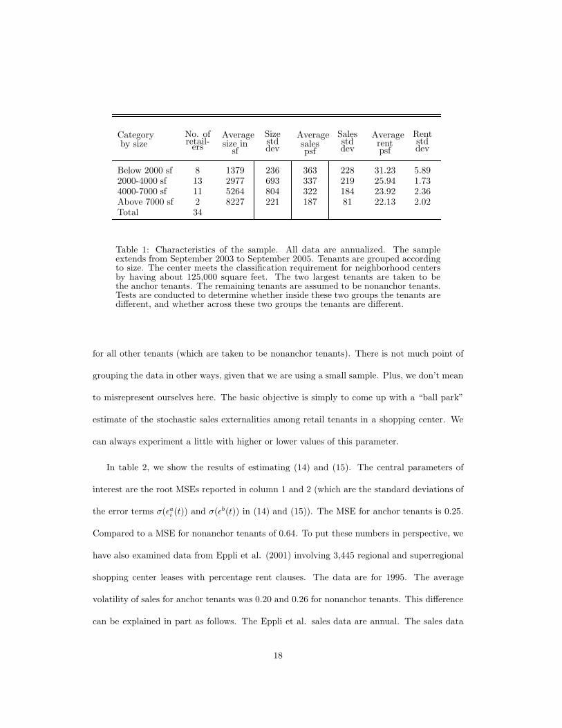
Below 2000 sf 8 1379 236 363 228 31.23 5.892000-4000 sf 13 2977 693 337 219 25.94 1.734000-7000 sf 11 5264 804 322 184 23.92 2.36Above 7000 sf 2 8227 221 187 81 22.13 2.02Total 34

Table 1: Characteristics of the sample. All data are annualized. The sampleextends from September 2003 to September 2005. Tenants are grouped accordingto size. The center meets the classification requirement for neighborhood centersby having about 125,000 square feet. The two largest tenants are taken to bethe anchor tenants. The remaining tenants are assumed to be nonanchor tenants.Tests are conducted to determine whether inside these two groups the tenants aredifferent, and whether across these two groups the tenants are different.

for all other tenants (which are taken to be nonanchor tenants). There is not much point of

grouping the data in other ways, given that we are using a small sample. Plus, we don’t mean

to misrepresent ourselves here. The basic objective is simply to come up with a “ball park”

estimate of the stochastic sales externalities among retail tenants in a shopping center. We

can always experiment a little with higher or lower values of this parameter.

In table 2, we show the results of estimating (14) and (15). The central parameters of

interest are the root MSEs reported in column 1 and 2 (which are the standard deviations of

the error terms σ(εai (t)) and σ(εb(t)) in (14) and (15)). The MSE for anchor tenants is 0.25.

Compared to a MSE for nonanchor tenants of 0.64. To put these numbers in perspective, we

have also examined data from Eppli et al. (2001) involving 3,445 regional and superregional

shopping center leases with percentage rent clauses. The data are for 1995. The average

volatility of sales for anchor tenants was 0.20 and 0.26 for nonanchor tenants. This difference

can be explained in part as follows. The Eppli et al. sales data are annual. The sales data

18

Anchor Nonanchor

f1 2.76(31.62)

f2 2.33(26.53)

x1 4.51(5.24)

x2 4.79(5.09)

x3 4.75(4.66)

t 0.0045 0.0061(0.84) (1.71)

ln(Qi) -0.21(-1.76)

W 0.65 0.63(4.90) (6.87)

Root MSE 0.25 0.64R2 0.99 0.96

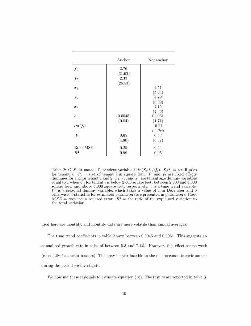
Table 2: OLS estimates. Dependent variable is ln(Si(t)/Qi). Si(t) = retail salesfor tenant i. Qi = size of tenant i in square feet. f1 and f2 are fixed effectsdummies for anchor tenant 1 and 2. x1, x2, and x3 are tenant size dummy variablesequal to 1 when Qi for tenant i is below 2,000 square feet, between 2,000 and 4,000square feet, and above 4,000 square feet, respectively. t is a time trend variable.W is a seasonal dummy variable, which takes a value of 1 in December and 0otherwise. t-statistics for estimated parameters are presented in parameters. RootMSE = root mean squared error. R2 = the ratio of the explained variation tothe total variation.

used here are monthly, and monthly data are more volatile than annual averages.

The time trend coefficients in table 2 vary between 0.0045 and 0.0061. This suggests an

annualized growth rate in sales of between 5.3 and 7.4%. However, this effect seems weak

(especially for anchor tenants). This may be attributable to the macroeconomic environment

during the period we investigate.

We now use these residuals to estimate equation (16). The results are reported in table 3.

19

Coefficientestimates

εa1(t) 0.26(2.19)

εa2(t) 0.23(1.98)

Root MSE 0.64R2 0.02

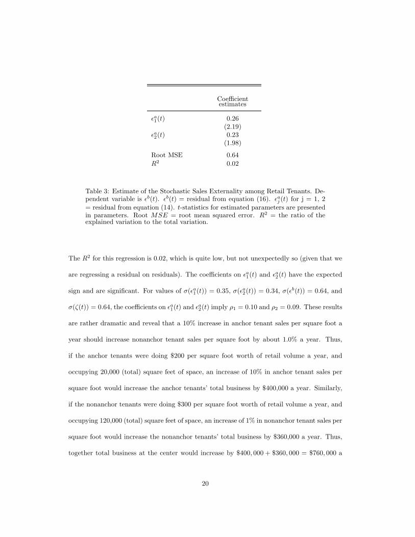
Table 3: Estimate of the Stochastic Sales Externality among Retail Tenants. De-pendent variable is εb(t). εb(t) = residual from equation (16). εaj (t) for j = 1, 2= residual from equation (14). t-statistics for estimated parameters are presentedin parameters. Root MSE = root mean squared error. R2 = the ratio of theexplained variation to the total variation.

The R2 for this regression is 0.02, which is quite low, but not unexpectedly so (given that we

are regressing a residual on residuals). The coefficients on εa1(t) and εa2(t) have the expected

sign and are significant. For values of σ(εa1(t)) = 0.35, σ(εa2(t)) = 0.34, σ(εb(t)) = 0.64, and

σ(ζ(t)) = 0.64, the coefficients on εa1(t) and εa2(t) imply ρ1 = 0.10 and ρ2 = 0.09. These results

are rather dramatic and reveal that a 10% increase in anchor tenant sales per square foot a

year should increase nonanchor tenant sales per square foot by about 1.0% a year. Thus,

if the anchor tenants were doing $200 per square foot worth of retail volume a year, and

occupying 20,000 (total) square feet of space, an increase of 10% in anchor tenant sales per

square foot would increase the anchor tenants’ total business by $400,000 a year. Similarly,

if the nonanchor tenants were doing $300 per square foot worth of retail volume a year, and

occupying 120,000 (total) square feet of space, an increase of 1% in nonanchor tenant sales per

square foot would increase the nonanchor tenants’ total business by $360,000 a year. Thus,

together total business at the center would increase by $400, 000 + $360, 000 = $760, 000 a

20

year, which is an additional $0.90 a year in purchases at the nonanchor tenant stores per

every additional $1 a year in purchases at the anchor tenant stores.

We can now use this information about ρ1 and ρ2 in a ceteris paribus analysis to simulate

the distribution of sales that would prevail if anchor tenants convey a positive sales externality

on nonanchor tenants. The simulated sales are generated assuming µ = .03, σ = .30, ρij = 0

(i.e., nonanchor tenants confer no externalities on the anchors), and S(0) = $200 per square

foot for a typical anchor tenant and µ = .03, σ = .50, ρji = 0.20, and S(0) = $300 per square

foot for a nonanchor tenant.

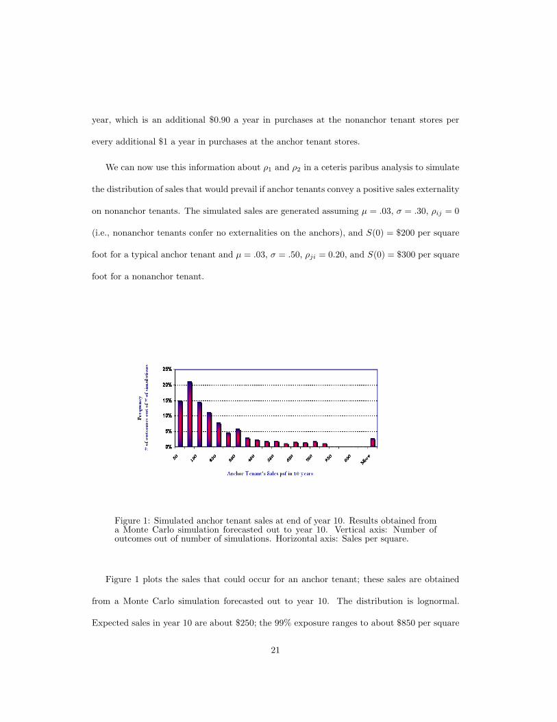
Figure 1: Simulated anchor tenant sales at end of year 10. Results obtained froma Monte Carlo simulation forecasted out to year 10. Vertical axis: Number ofoutcomes out of number of simulations. Horizontal axis: Sales per square.

Figure 1 plots the sales that could occur for an anchor tenant; these sales are obtained

from a Monte Carlo simulation forecasted out to year 10. The distribution is lognormal.

Expected sales in year 10 are about $250; the 99% exposure ranges to about $850 per square

21

foot.

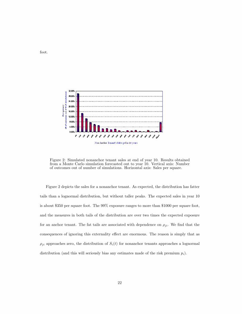
Figure 2: Simulated nonanchor tenant sales at end of year 10. Results obtainedfrom a Monte Carlo simulation forecasted out to year 10. Vertical axis: Numberof outcomes out of number of simulations. Horizontal axis: Sales per square.

Figure 2 depicts the sales for a nonanchor tenant. As expected, the distribution has fatter

tails than a lognormal distribution, but without taller peaks. The expected sales in year 10

is about $350 per square foot. The 99% exposure ranges to more than $1000 per square foot,

and the measures in both tails of the distribution are over two times the expected exposure

for an anchor tenant. The fat tails are associated with dependence on ρji. We find that the

consequences of ignoring this externality effect are enormous. The reason is simply that as

ρji approaches zero, the distribution of Si(t) for nonanchor tenants approaches a lognormal

distribution (and this will seriously bias any estimates made of the risk premium pi).

22

8. Specification of Production Parameters and Lease Contract Terms

There are eight remaining exogenous variables that need to be specified: the four produc-

tion parameters Qi, Q−i = {Q1, Q2, . . . , Qi−1, Qi+1, . . . , Qn}, λi, and γji, and the four lease

contract terms αi, βi, S, and Si(0). The values of λi and γji are not observed; however,

these values (along with Qi, Q−i = {Q1, Q2, . . . , Qi−1, Qi+1, . . . , Qn}) can be inferred. Be-

cause Si(t) = Di(t) ·Xi(t)Qλi

i

∏

j 6=i

Qγji

j applies for all t, we can substitute the value Si(0) for

YiQλi

i

∏j 6=i Q

γji

j , and plug this result back into our model; thereby eliminating the specifica-

tion of Qi, Q−i = {Q1, Q2, . . . , Qi−1, Qi+1, . . . , Qn}, λi, and γji.

The four lease contract terms αi, βi, S, and Si(0) are chosen to be consistent with the

data. We set αi = $30 per square foot, βi = 0.07, S = $400 per square foot, and Si(0) = $300

per square foot for percentage rent contracts. The simulation model is then coded with

the demand shock parameters, the rate of economic depreciation, the initial sales level, the

discount rate and risk premium, the liquidation value, and an assumed value of V = $265 per

square foot and solved for an equivalent fixed rent for a pure fixed rent contract. The solution

was $40.26 per square assuming a nonexistent probability of default.

9. Some Simulation Results

Here we present a number of simulations to illustrate the basic workings of the model.

9.1 Increase in Sales Percentage Rate

Figure 3 depicts the value of four different lease contracts, and illustrates the effect of varying

the percentage rental rate for each one of these leases. The four different lease contracts

depicted are: op(1, 0) denotes a pure fixed rent contract with default; op(0, 0) denotes a pure

fixed rent contract without default; we use op(1, 1) to denote a percentage rent contract

23

with default; and op(0, 1) to denote a percentage rent contract without default. This vector

notation is convenient (and will be used throughout the remainder of the paper), the first

argument denotes with default (= 1) or without default (= 0); the second argument denotes

a pure fixed rent contract (= 0) or a percentage rent contract (= 1).

Figure 3: Simulated increase in sales percentage rate on the value of a retaillease. Results obtained from a Monte Carlo simulation. Vertical axis: Value ofretail lease (V ). Horizontal axis: Sales percentage rate (βi). op(1, 0) denotes apure fixed rent contract with default; op(0, 0) denotes a pure fixed rent contractwithout default; we use op(1, 1) to denote a percentage rent contract with default;and op(0, 1) to denote a percentage rent contract without default.

Each point on the graph should be thought of as a separate lease contract with a different

sales percentage rate. The value of a pure (default-free) fixed rent contract in this case is

invariant with respect to a change in sales percentage rate βi; which is no big surprise. Also

no big surprise, op(0, 0 shows up in β−V space as above op(1, 0). This comparison is a pretty

trivial example.

24

Comparing op(0, 1) and op(0, 0) is, however, nontrivial. The results suggest (ignoring

default) that a percentage rent clause is of positive value to a shopping center owner, but

negative to a tenant. Furthermore, the results suggest that a percentage rent clause can

perhaps add substantial value; maybe as much as 50% or more.

This comparison, however, overlooks a vital fact – the tenant’s embedded default option.

This embedded option to leave the center is of positive value to the tenant, but negative to the

shopping center owner. Furthermore, for small values of βi, the value of this option can more

than offset the full value of percentage rent clause, causing op(1, 1) to fall below op(0, 0). For

large values of βi, the opposite result holds: the value of the percentage rent clause more than

offsets the tenant’s option to default; which makes sense. The two options are not linearly

related; together, they are a compound option.

Next, if you think about it, what figure 3 shows is that for moderate values of βi the values

of these two options are such that one may simply give them little or no weight for purposes

of, say, financing, and simply discount the fixed guaranteed minimum rent to arrive at value

(compare op(1, 1) and op(0, 0) for moderate values of βi). This finding, oddly enough, helps

to explain why, in practice, many lenders give little or no value to straight percentage of sales

rentals for the purpose of financing. Oddly, enough, these lenders appear to be getting values

right, but perhaps for the wrong reasons.

What is also interesting about figure 3 is that it offers a somewhat latent role for percentage

of sales rentals: namely, to offset the negative value to center owners of the tenant’s option

to default.

25

9.2 Increase in Volatility

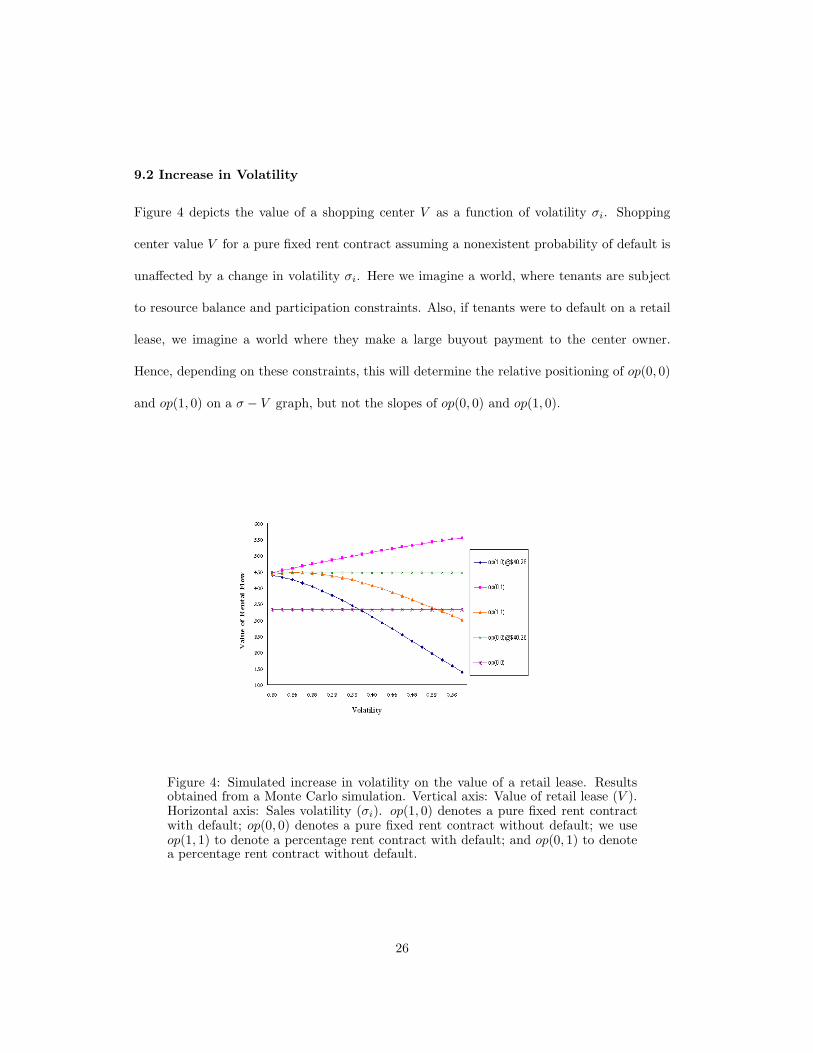
Figure 4 depicts the value of a shopping center V as a function of volatility σi. Shopping

center value V for a pure fixed rent contract assuming a nonexistent probability of default is

unaffected by a change in volatility σi. Here we imagine a world, where tenants are subject

to resource balance and participation constraints. Also, if tenants were to default on a retail

lease, we imagine a world where they make a large buyout payment to the center owner.

Hence, depending on these constraints, this will determine the relative positioning of op(0, 0)

and op(1, 0) on a σ − V graph, but not the slopes of op(0, 0) and op(1, 0).

Figure 4: Simulated increase in volatility on the value of a retail lease. Resultsobtained from a Monte Carlo simulation. Vertical axis: Value of retail lease (V ).Horizontal axis: Sales volatility (σi). op(1, 0) denotes a pure fixed rent contractwith default; op(0, 0) denotes a pure fixed rent contract without default; we useop(1, 1) to denote a percentage rent contract with default; and op(0, 1) to denotea percentage rent contract without default.

26

V for a percentage rent contract, however, declines as σ increases. Others suggest that V

should increase as σ increases; uncertainty raises the value of a percentage rent clause. This

prediction ignores, however, risk considerations and possible externalities. After controlling

for these two effects, we find that V decreases as σi increases. This occurs because the tenant’s

option to default more than offsets the value of a percentage rent clause. This is especially

true for moderate to large values of σi; compare op(1, 1) to op(1, 0) for values of σi between,

say, 0.4 and 0.6. For small values of σi, however, V appears to increase as σi increases, but

by not by much; compare op(1, 1) to op(0, 1) for values of σi between 0.2 and 0.25. This,

again, illustrates the point that, together, the tenant’s option to default and the percentage

rent clause are compound options.

9.3 Increase in Sales Percentage Rate and Sales Threshold Level

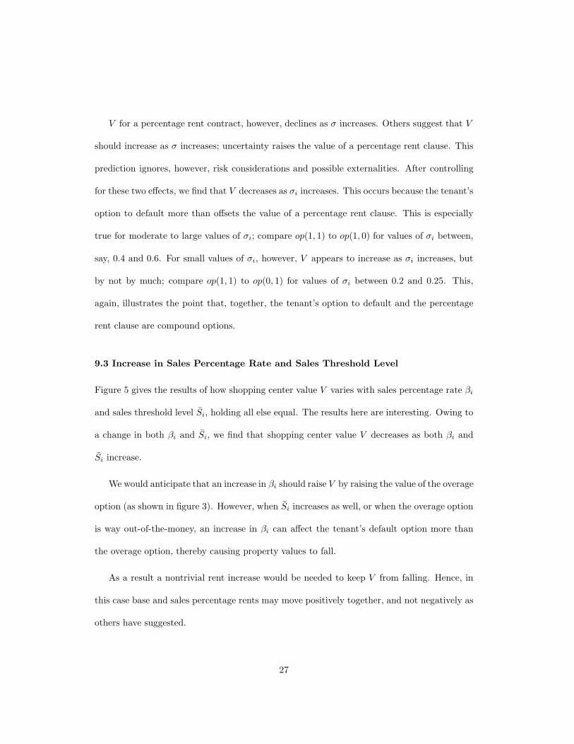
Figure 5 gives the results of how shopping center value V varies with sales percentage rate βi

and sales threshold level Si, holding all else equal. The results here are interesting. Owing to

a change in both βi and Si, we find that shopping center value V decreases as both βi and

Si increase.

We would anticipate that an increase in βi should raise V by raising the value of the overage

option (as shown in figure 3). However, when Si increases as well, or when the overage option

is way out-of-the-money, an increase in βi can affect the tenant’s default option more than

the overage option, thereby causing property values to fall.

As a result a nontrivial rent increase would be needed to keep V from falling. Hence, in

this case base and sales percentage rents may move positively together, and not negatively as

others have suggested.

27

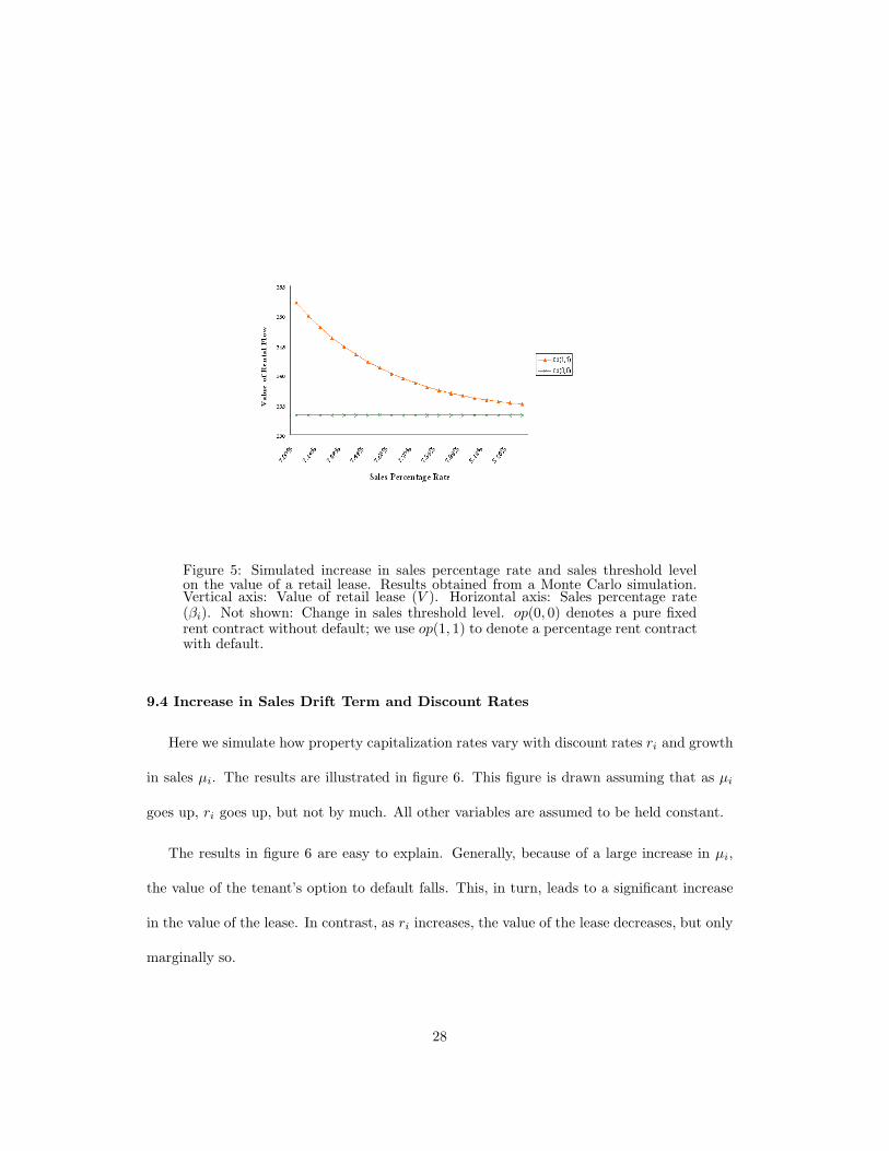
Figure 5: Simulated increase in sales percentage rate and sales threshold levelon the value of a retail lease. Results obtained from a Monte Carlo simulation.Vertical axis: Value of retail lease (V ). Horizontal axis: Sales percentage rate(βi). Not shown: Change in sales threshold level. op(0, 0) denotes a pure fixedrent contract without default; we use op(1, 1) to denote a percentage rent contractwith default.

9.4 Increase in Sales Drift Term and Discount Rates

Here we simulate how property capitalization rates vary with discount rates ri and growth

in sales µi. The results are illustrated in figure 6. This figure is drawn assuming that as µi

goes up, ri goes up, but not by much. All other variables are assumed to be held constant.

The results in figure 6 are easy to explain. Generally, because of a large increase in µi,

the value of the tenant’s option to default falls. This, in turn, leads to a significant increase

in the value of the lease. In contrast, as ri increases, the value of the lease decreases, but only

marginally so.

28

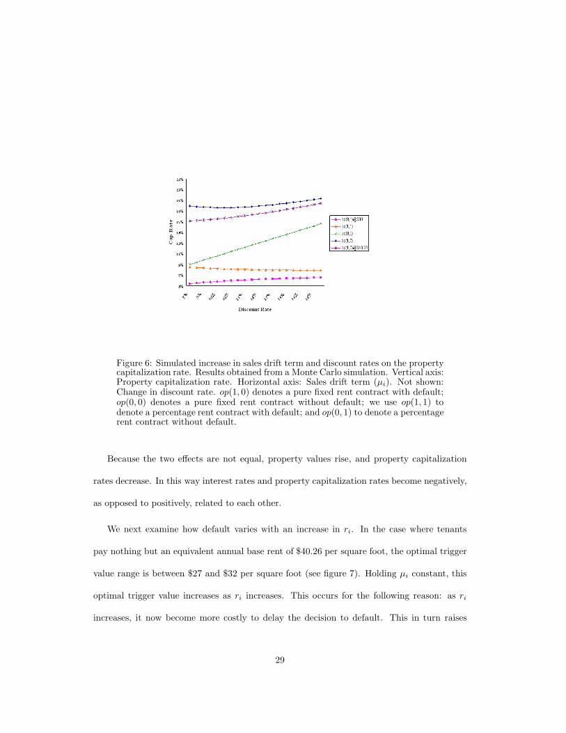
Figure 6: Simulated increase in sales drift term and discount rates on the propertycapitalization rate. Results obtained from a Monte Carlo simulation. Vertical axis:Property capitalization rate. Horizontal axis: Sales drift term (µi). Not shown:Change in discount rate. op(1, 0) denotes a pure fixed rent contract with default;op(0, 0) denotes a pure fixed rent contract without default; we use op(1, 1) todenote a percentage rent contract with default; and op(0, 1) to denote a percentagerent contract without default.

Because the two effects are not equal, property values rise, and property capitalization

rates decrease. In this way interest rates and property capitalization rates become negatively,

as opposed to positively, related to each other.

We next examine how default varies with an increase in ri. In the case where tenants

pay nothing but an equivalent annual base rent of $40.26 per square foot, the optimal trigger

value range is between $27 and $32 per square foot (see figure 7). Holding µi constant, this

optimal trigger value increases as ri increases. This occurs for the following reason: as ri

increases, it now become more costly to delay the decision to default. This in turn raises

29

the optimal trigger value (although the range is quite small for the parameter values used in

these calculations). Next, a ceteris paribus increase in the optimal trigger value lowers the

property price, which would raise the capitalization rate. So with a large enough increase in

ri, interest rates and property capitalization rates could go back to being positively related

to each other.

Figure 7: Optimal trigger value as a function of the discount rate. Results obtainedfrom a Monte Carlo simulation. Vertical axis: Discount rate (r). Horizontal axis:Optimal default trigger value. op(1, 0) denotes a pure fixed rent contract withdefault; we use op(1, 1) to denote a percentage rent contract with default; andop(0, 1) to denote a percentage rent contract without default.

By comparison when tenants pay a percentage rent, the optimal trigger values are generally

between $25 and $30 per square foot. These lower trigger values mean that property prices

are higher (less default risk) and capitalization rates are lower.

Since the optimal trigger values are declining in opportunity costs, property values are

30

even higher for pure fixed rent contracts at an annual base rent of $30 per square foot, which

also makes sense. But, of course, we don’t expect to observe such contracts in the market.

9.5 Increase in Stochastic Sales Externality Risk Premium

At the start of the paper we said that the usual theory for measuring the user cost of

a retail lease as the sum of the expected risk-adjusted discount rate, plus the depreciation

incurred and minus the rate of asset price change no longer applies. Rather the user cost

needs to include a risk premium to compensate the owner/tenant for the risk that the sales

externality effects at the center could dissipate or disappear over time. We also said that

ignoring this risk premium may significantly overestimate shopping center value. Here we

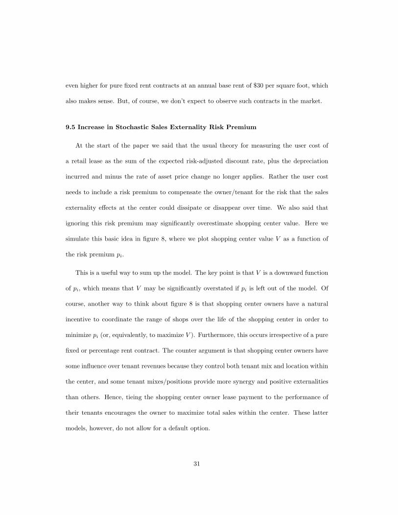
simulate this basic idea in figure 8, where we plot shopping center value V as a function of

the risk premium pi.

This is a useful way to sum up the model. The key point is that V is a downward function

of pi, which means that V may be significantly overstated if pi is left out of the model. Of

course, another way to think about figure 8 is that shopping center owners have a natural

incentive to coordinate the range of shops over the life of the shopping center in order to

minimize pi (or, equivalently, to maximize V ). Furthermore, this occurs irrespective of a pure

fixed or percentage rent contract. The counter argument is that shopping center owners have

some influence over tenant revenues because they control both tenant mix and location within

the center, and some tenant mixes/positions provide more synergy and positive externalities

than others. Hence, tieing the shopping center owner lease payment to the performance of

their tenants encourages the owner to maximize total sales within the center. These latter

models, however, do not allow for a default option.

31

Figure 8: Simulated increase in stochastic sales externality risk premium on thevalue of a retail lease. Results obtained from a Monte Carlo simulation. Verticalaxis: Value of retail lease (V ). Horizontal axis: Stochastic sales externality riskpremium (pi). Not shown: Change in discount rate. op(1, 0) denotes a pure fixedrent contract with default; op(0, 0) denotes a pure fixed rent contract withoutdefault; we use op(1, 1) to denote a percentage rent contract with default; andop(0, 1) to denote a percentage rent contract without default.

10. Conclusions

In this paper we have provided a general formulation for valuing a retail shopping center under

uncertainty. We then analyzed the effects of changes in sales percentage rates, uncertainty,

sales threshold levels, sales drift terms, discount rates, and risk premia on valuation.

Our model differs from previous studies in a number of ways. Previous studies in the

literature are concerned either with inter-store externalities (and with showing that center

owners need to allocate as much as 60% of the space at the center to large major retailers

at low rents in order to maximize total revenues at the center), or with the pricing of retail

32

leases in a framework in which sales follow a stochastic process. These models typically ignore

feedback effects, such as the loss of a major tenant (or a decline in the tenant’s customer

drawing power) on sales, occupancy rates, and rent levels of the other tenants. We in this

paper are concerned with an environment in which sales are stochastic; rents are set in a

competitive market; tenants confer a positive externality on each other; and in which defaults

can occur. We then use the model to show that the usual certainty theory for measuring the

user cost of a retail lease as the sum of the expected risk-adjusted discount rate, plus the

depreciation incurred and minus the rate of asset price change no longer applies; instead, one

needs to discount at a slightly higher discount rate to compensate the owner/tenant for the

risk that the sales externality effects at the center could dissipate or disappear over time.

Several other features of the above theory are perhaps worthy of notice. First, ignoring

these feedback effects means that shopping center valuations are perhaps too high and prop-

erty capitalization rates are too low. Second, it is a feature of the theory that a percentage

rent clause is of positive value to a shopping center owner, but negative to a tenant. It is also

a feature of the theory that the tenant’s embedded default option is of positive value to the

tenant, but negative to the shopping center owner. Generally, we find that these two options

offset one another, thereby offering a perhaps somewhat latent role for percentage of sales

rentals: to offset the negative value to center owners of the tenant’s embedded default option.

It is also a feature of the theory that shopping center owners have a natural incentive to

coordinate the merchandise mix of the shops over the life of the shopping center in order to

minimize the value of the tenant’s embedded default option. This is an important point, a

point that has gone unnoticed.

Even though the model is relatively simple, it helps to explain a variety of phenomena

33

ranging from an increase in sales volatility may reduce, rather than increase, shopping center

value, as others have suggested; why base and percentage rents may move positively together,

and not negatively as others have suggested; why retail property capitalization rates and in-

terest rates can be negatively, as opposed to positively, related with each other; and why leases

with a percentage of sales rental are often given little or no value for purposes of financing

by lenders, regardless of whether or not the tenant is a national chain with substantial net

worth.

34

11. References

1. Benjamin John D., Boyle Glenn W. and Sirmans C.F., Retail Leasing: The Determi-nants of Shopping Center Rents. AREUEA Journal 18(3) 1990 pp. 302-312.

2. Benjamin, John D., Boyle Glenn W. and Sirmans C.F., Price Discrimination in Shop-ping Center Leases. Journal of Urban Economics 32, 1992, pp 299-317.

3. Benjamin John D. and Chinloy Peter, The Structure of a Retail Lease Journal of RealEstate Research 26(2) 2004 pp. 223-236.

4. Brueckner, Jan K., Inter-Store Externalities and Space Allocation in Shopping Centers.Journal of Real Estate Finance and Economics 7 1993 pp.5-16.

5. Clapham, Eric, A Note on Embedded Lease Options Journal of Real Estate Research25(3) 2003 pp. 347-359.

6. Colwell, Peter F and Munneke, Henry J., Percentage Lease and the Advantages of Re-gional Malls. Journal of Real Estate Research, 15(3), 1998, pp. 239-252.

7. Eppli, Mark J., Hendershott Patric H., Mejia, Louis C. and Shilling, James D., Base andOverage Rent Clauses in Retail Leases: Motivation and Use, University of WisconsinWorking Paper, 2001.

8. Gatzlaff, Dean H., Sirmans, G. Stacy, and Diskin, Barry A., The Effect of Anchor Ten-ant Loss on Shopping Center Rents, Journal of Real Estate Research 9 (1994) pp. 99-110.

9. Gould, Eric C., Pashigian, Peter B., and Prendergast, Canice J., Contracts, Externali-ties, and Incentives in Shopping Malls Review of Economics and Statistics, 87(3), 2005pp. 411-422.

10. Grenadier, Steven R., Valuing Lease Contracts: A Real-Option Approach Journal ofFinancial Economics 38 1995 pp.297-331.

11. Hendershott, Patric H. and Ward, Charles, Incorporating Option-like Features in theValuation of Shopping Centers Real Estate Finance Winter 2000 pp. 31-36.

35

12. Hendershott, Patric H. and Ward, Charles, Valuing and Pricing Retail Leases with Re-newal and Overage Options Journal of Real Estate Finance and Economics 26(2/3) 2003pp. 223-240.

13. Kozloff, Emme, Retail: Tackling the Biggest Operating Expense, Labor, With Work-force Management Tools, Bernstein Research Call, 2005.

14. Lee, Kangoh, Optimal Retail Lease Contracts: The Principal-Agent Approach RegionalScience and Urban Economics 25 1995 pp.727-738.

15. Miceli, Thomas J. and Sirmans, C.F., Contracting with Spatial Externalities and AgencyProblems. Regional Science and Urban Economics 25 1995 pp. 355-372.

16. Mooradian, Yang and Yang, Shiawee X. Cancelation Strategies in Commercial Real Es-tate Leasing. Real Estate Economics 28(1) 2000 pp. 65-88.

17. Pashigian, Peter B. and Gould, Eric D. Internalizing Externalities: The Pricing of Spacein Shopping Malls. Journal of Law and Economics 1998 pp. 115-142.

18. Riddiough, Timothy, and Williams, Joseph, Optimal Contracting on Retail Space, Uni-versity of Wisconsin Working Paper, 2005.

19. Shilling, James D. Is Their a Risk Premium Puzzle in Real Estate? Real Estate Eco-nomics, 31 (3) 2003 pp. 315-330.

20. Wheaton, William C. Percentage Rent in Retail Leasing: The Alignment of Landlord-Tenant Interests. Real Estate Economics 28(2) 2000 pp.185-204.

36

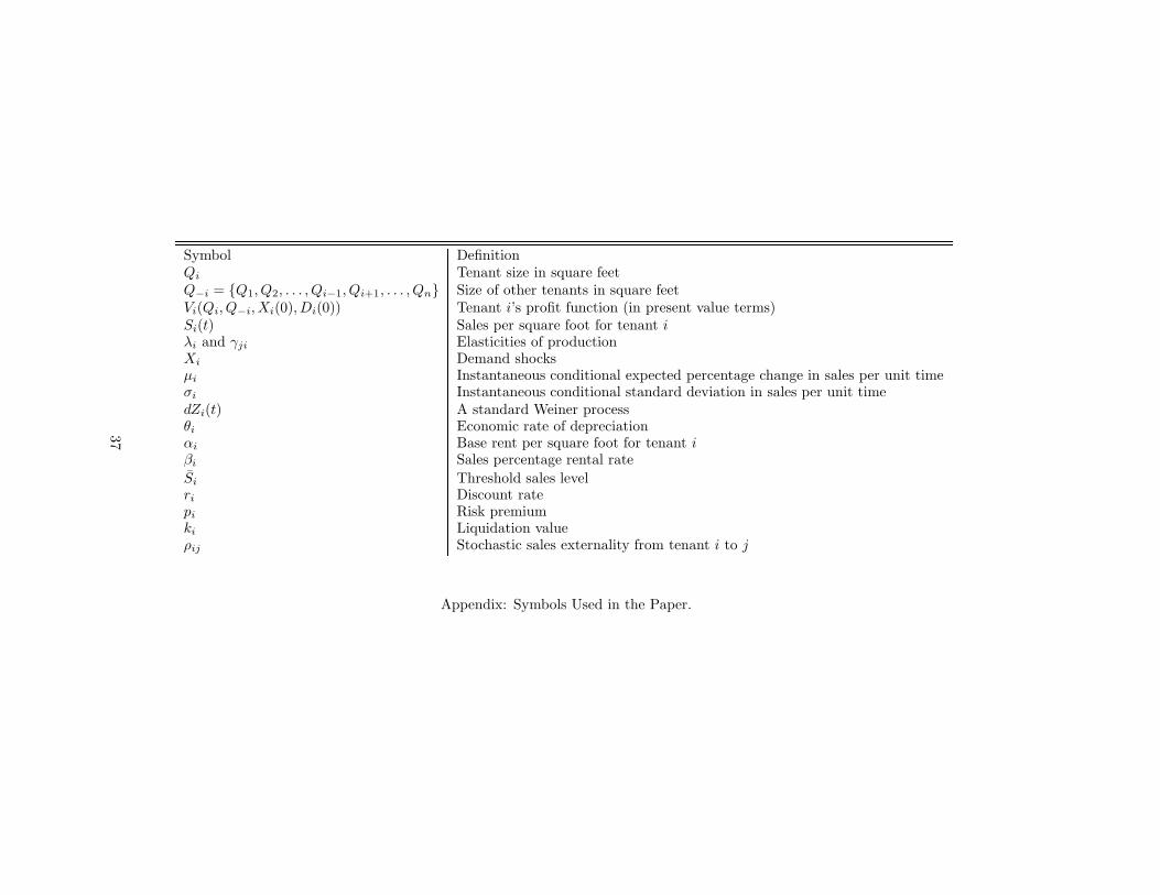
Symbol DefinitionQi Tenant size in square feetQ−i = {Q1, Q2, . . . , Qi−1, Qi+1, . . . , Qn} Size of other tenants in square feetVi(Qi, Q−i, Xi(0), Di(0)) Tenant i’s profit function (in present value terms)Si(t) Sales per square foot for tenant iλi and γji Elasticities of productionXi Demand shocksµi Instantaneous conditional expected percentage change in sales per unit timeσi Instantaneous conditional standard deviation in sales per unit timedZi(t) A standard Weiner processθi Economic rate of depreciationαi Base rent per square foot for tenant iβi Sales percentage rental rateSi Threshold sales levelri Discount ratepi Risk premiumki Liquidation valueρij Stochastic sales externality from tenant i to j

Appendix: Symbols Used in the Paper.

37