Value-Relevance of Accounting Information for Intangible...

Value-Relevance of Accounting Information for Intangible-Intensive

Industries and the Impact of Scale Factor

Mustafa Ciftci Binghamton University, SUNY

School of Management PO Box 6000

Binghamton, NY 13902-6000 [email protected]

March 2010



Abstract

Prior research suggests that accounting information is not useful when valuing firms

with large amount of intangibles (Amir and Lev (1996)). However, using R2 from

regression of earnings and book values on prices, Collins et al. (1997) (hereafter CMW)

find that value-relevance for intangible-intensive industries is as high as not intangible-

intensive. An explanation for the discrepancy between Amir and Lev (1996) and CMW is

that the high value-relevance for intangible-intensive industries documented by CMW is

due to not controlling for the differences in scale (Brown et al. (1999)). Consistent with

this explanation, we find that, once we control for scale factor, R2 is approximately 30%

lower for intangible-intensive than not intangible-intensive industries. In addition, we

find that the intertemporal decline in value-relevance for all industries documented by

Brown et al. (1999) is due to intangible-intensive industries suggesting that intangible-

intensive industries are substantially affecting the evolution of characteristics of financial

reporting system as a whole.



I. Introduction

In this paper we investigate the value-relevance of accounting information for

intangible-intensive and not intangible-intensive industries. US GAAP does not allow the

capitalization of research and development (R&D) expenditures and most of other

intangibles, while it allows the capitalization of capital of expenditures.1 The asymmetric

treatment of intangibles has been heavily criticized in prior literature. Amir and Lev

(1996) argue that financial accounting information is of limited usefulness to investors

when valuing technology and pharmaceutical companies that invest heavily in

intangibles. However, CMW find that value-relevance of accounting information for

intangible-intensive industries is as high as not intangible-intensive. Similarly, Francis

and Schipper (1999) also did not find economically significant difference in value-

relevance of accounting information between high-tech and low-tech industries.

Consequently, the evidence in CMW is not consistent with the arguments in Amir and

Lev (1996). One explanation given by Lev and Zarowin (1999) for this discrepancy is

that the expensing of R&D expenditures on average should not necessarily lead to lower

value-relevance for intangible-intensive industries. They state that if firms in intangible

intensive-industries are on average in R&D steady state, accounting information on

average should not be distorted for them.

1 Lev (2001) R&D is the most important intangibles. Thus, we will primarily focus about the accounting treatment of R&D in our arguments.

2

We try to shed light on the conflicting evidence in prior literature about the

informational deficiencies for intangible-intensive firms. We use data from Compustat

and CRSP between 1975 and 2006 available in 2008 tapes. We first explore whether the

earnings and book values for intangible intensive industries are distorted for intangible-

intensive industries. We find that the mean earnings (book values) are 62% (20%) greater

under capitalization than that under expensing of R&D for intangible-industries,

suggesting that accounting information in intangible-intensive industries is on average

heavily distorted. An alternative explanation for the high value-relevance for intangible-

intensive industries documented by CMW is omitting a variable from the regression

which is correlated with variables included. Brown et al. (1999) argue that lack of control

for the variation in scale factor might bias the R2 from regression of prices with earnings

and book values. They analytically show that CV (coefficient of variation) of scale factor

is positively related to R2 from price regressions. Following the arguments in Brown et al.

(1999), we find that the CVs of scale factor proxies are 27%-32% larger for intangible-

intensive industries than not intangible-intensive.

We then explore the impact scale factor on value-relevance of accounting

information. Without including CVs of scale factor proxies, consistent with CMW, we

did not find any significant difference in value-relevance between intangible-intensive

and not intangible-intensive industries (R2s for both groups are around 58-60%).

However, when we include CVs of scale factor proxies, we find that R2 for intangible-

intensive is 18% less than not intangible-intensive industries, suggesting that R2 is 30%

(18%/60%) smaller for intangible-intensive industries. In addition, to explore the impact

of capitalization on value-relevance, we adjust earnings and book values to eliminate the

impact of expensing of R&D, we find that the difference between two industry groups

3

decline by one third to 11.80%, indicating that indeed expensing reduces value-relevance

to some extent.

Brown et al. (1999) document that the increase in value-relevance of accounting

information documented by CMW and Francis and Schipper (1999) is due to increase CV

of scale factor over time and once we control for it, the value-relevance declines

intertemporally. We investigate whether the intertemporal decline in value-relevance of

accounting information for all firms documented by Brown et al. (1999) is driven by

intangible-intensive industries. Consistent with this expectation, we find that there is no

statistically significant decline in value-relevance of accounting information for not

intangible-intensive industries, whereas there is a significant decline for intangible-

intensive.

The findings in this paper have important implication for the debate about the

accounting treatment of intangible assets and the information environment for intangible-

intensive industries. Intangible-intensive companies are playing an unprecedented role in

US economy in the last three decades. Chan et al. (2001) state that technology-based

firms and pharmaceutical industry together account for 40% of the value of the S&P500.

Considering the enormous role played by intangible-intensive firms in today�’s economy,

an important issue is whether the current accounting system satisfies the informational

needs of investors with respect to intangibles. In fact SEC recently announced a proposed

schedule to adopt International Financial Reporting System (IFRS) in the US which

allows capitalization of development costs (IAS 38). The findings in this paper suggest

that indeed the accounting information is less useful for intangible-intensive industries

and raise the possibility that switching to IFRS might improve value-relevance for

intangible-intensive industries.

4

Our paper also contributes to the literature investigating the intertemporal trends in

value-relevance of accounting information. Brown et al. (1999) document an

intertemporal decline once we control the variation in scale factor. Core et al. (2003)

document a substantially low value-relevance in recent �“New Economy�” sub-period,

1995-1999. However, it is not clear whether the decline in value-relevance in the new

economy sub-period is temporary or permanent. We show that intertemporal pattern for

all industries documented by Brown et al. is due to intangible-intensive industries and

that the low value-relevance in the new economy sub-period is temporary and it reverts

back to its prior levels after 2002.

This paper also contributes to the recent line of research which indicates that

intangible-intensive firms are increasingly affecting the overall characteristics of the

information produced by financial reporting system. Darrouh and Ye (2007) underline the

importance unrecorded intangibles in resolving the puzzling negative relationship

between market values and earnings for loss firms. Similarly, Franzen et al. (2007)

documents the impact of unrecorded R&D on measures of distress risk such as Altman z-

score. These studies suggest intangible-intensive firms increasingly affecting

characteristics of financial reporting system as a whole. We contribute this line of

research by documenting that when it comes to intertemporal trends in value-relevance of

accounting information, intangible-intensive firms also play a significant role. In fact,

given the recent evidence by Dichev and Tang (2008) that there is a decline in matching

of revenues and expenses, intangible-intensive firms might be also responsible for this

decline as well.

The rest of the paper is organized as follows. Section 2 provides the literature

review and research questions. Section 3 presents research design and section 4 sample

5

description and descriptive statistics. Section 5 presents results and finally section 6

concludes the paper.

2. Literature Review and Research Questions

2.1. Value-relevance of Accounting Information for Intangible-intensive Industries

In today�’s economy intangible assets play a role as important as physical and

financial assets. Federal Reserve economist Nakamura states that �“U.S. companies spend

annually on intangibles is on par with total corporate investment in physical assets.�”2

The growing importance of intangibles in the economy in the last three decades attracted

the attention of academia to issues related to these assets. An important type of intangible

asset is R&D. Prior research documents that R&D expenditures are associated with future

earnings, suggesting that these expenditures have future benefits like other assets (Lev

and Sougiannis, 1996). However, Generally Accepted Accounting Principles (U.S.

GAAP) do not treat R&D expenditures as assets, and require them to be expensed as

incurred. Several researchers raise concern about the usefulness of financial information

due to expensing of R&D. Even though R&D is immediately expensed, the benefits

associated with R&D are realized much later and are not matched previously expensed

R&D expenditures. Consequently, the primary accounting principle of matching revenues

with expenses is seriously distorted (Lev and Zarowin, 1999).

Amir and Lev (1996) argue that while intangible assets contribute to the market

value of these firms, current accounting rules do not allow recording these assets.

Consequently information provided in financial statements is not useful to investor when

valuing the firms with large amounts of intangible assets. Amir and Lev (1996) find that

2 Lev (2001)

6

earnings, book values and cash flows are largely irrelevant on a stand-alone basis when

valuing companies in the cellular telephone industry. They further state that �“the

accounting measurement and reporting system is ill-equipped to provide value-relevant

information in emerging high-tech industries, such as wireless communications.

However, they did no explore whether their results apply to all intangible-intensive

industries. However, CMW document that the R2 from regression of earnings and book

values on prices is slightly greater for intangible-intensive industries than not intangible-

intensive industries. Similarly, Francis and Schipper (1999) show that high-tech firms

have similar value-relevance compared to low-tech firms. Thus, the arguments in Amir

and Lev (1996) are in conflict with the evidence provided by CMW and Francis Schipper

(1999).

One explanation provided by Lev and Zarowin (1999) for the discrepancy between

Amir and Lev (1996) and CMW is that accounting numbers on average are not distorted

for intangible-intensive industries. They argue that in steady R&D state environment, the

immediate expensing of R&D will result in the same earnings as those based on R&D

capitalization. They further state that �“it is only when the investment rate on intangibles

changes over time that reported earnings based expensing will materially differ from

economics earnings based on capitalization.�” However, they do not clarify whether firms

in intangible-intensive-industries are on average in steady R&D state or whether

accounting information for firms in intangible-intensive industries are on average

distorted.

Another recent study in value-relevance on accounting information for intangible-

intensive firms is Monahan (2005). He investigates whether adjusting accounting

numbers for expensing of R&D improves value-relevance (i.e. R2). He finds that

7

capitalization leads to statistically significant increase in value-relevance only when a

firm has high future R&D growth and high conservatism (i.e. he measures conservatism

with the intensity of R&D capital to total asset ratio). However, he does not take into

account the impact of CV of scale factor when making comparisons across groups.

Moreover, he does not investigate the differences neither in value-relevance nor

intertemporal pattern in value-relevance between intangible-intensive and not intangible

intensive industries.

2.2. The Impact of Scale Factor on Value-Relevance

Brown et al. (1999) provide theoretical evidence about the impact of scale factor on

value-relevance. In a regression of earnings on prices R2 shows how much of the

variation in price can be explained by the variation in EPS. Hence, R2 seems to be

reasonable measure of value-relevance. Brown et al. (1999) argue that comparison of R2s

among different groups might be misleading if R2 is also affected by scale. To illustrate

the impact of scale on R2, we present the notation from Brown et al. (1999). Let us

assume following linear bivariate relationship between z = (z1,�…. zn) and w = (w1,�…. wn).

zi = a + b wi + ei (1)

Equation (1) is free of scale. In this model zi can be considered as value of a stock at

the end of a period and wi, the EPS in the period. In equation (1), R2 represents the

explanatory power of independent variable. On the other hand, a researcher usually can

merely observe scale-affected data. To observe the impact of scale now assume that data

is affected by a scale factor, s = (s1,�…. sn), then equation (1) becomes:

si zi = a si + b si wi + si ei (2)

8

Brown et al. (1999) show that R2 of the estimated relationship between z and w is

affected is affected by both the variation in s, scale-factor and variation in w. An example

for scale differences provided by Brown et al. (1999) is Berkshire Hataway, with a share

price of $45,000 and IBM, with a share price of $100. Researchers, such as CMW,

usually regress prices on accounting data such as EPS do not control for the impact of

scale effect. Thus, they estimate following model.

yi = + xi + gi (3)

Where

yi = si zi, xi = si wi, and gi = si ei,

In equation (3), asi is omitted, compared to equation (2), which would lead to

correlated omitted variable problem. Brown et al. (1999) show that omitting scale factor

in the above equation will bias not only the coefficient estimates but also the R2 from the

regression. Moreover, they analytically show that there is a positive relationship between

R2 and CV of scale factor. The stock splits share repurchases are endogenous corporate

choices which affect scale factor. In addition, differences in ROE and payout ratios also

affect scale factor. Thus, they suggest that when making comparisons among different

groups of interest based on R2, one has to control for scale. One way they suggest to

control variation in scale is regressing R2 from the price regression on CV of scale factor

proxies such as CV of price and book value.

2.3. Intertemporal Patterns in Value-Relevance of Accounting Information

There have been recent arguments that historical cost financial statements lost

value-relevance because of the shift from an industrialized economy to a high-tech,

service-oriented economy (CMW). CMW provided several reasons for the intertemporal

9

decline in value-relevance of accounting information. One reason they suggest is that

there is an increase in the number of intangible-intensive firms over time. Given the

argument in Amir and Lev (1996) that accounting information is less value-relevant for

firms in intangible-intensive industries, the intertemporal increase in the number of

intangible-intensive firms should lead to intertemporal decline in value-relevance of

accounting information. The other reason is the increase in the number of firms reporting

loss and increase in nonrecurring items over time. Elliot and Hanna (1996) and Hayn

(1995) suggest that negative earnings and nonrecurring items can adversely affect the

value-relevance of earnings. Based on this motivation, CMW investigates the

intertemporal pattern in value-relevance of accounting information over 41 years between

1953 and 1993. Contrary to the above claims, they find that the combined value-

relevance of earnings and book values increase over past 40 years rather than decline.

They, however, find that value-relevance of bottom line earnings has declined over time

having been replaced by an increase in value relevance of book values. Francis and

Schipper (1999) also provide similar intertemporal increase in value-relevance of

accounting information.

Brown et al. (1999) on the other hand, argue that the intertemporal increase in

combined value-relevance of earnings and book values documented by CMW is due to

scale effect which acts as a correlated omitted variable. They use CV of share price and

book value per share as proxy for CV of scale factor and document that, once we control

for scale factor, there is in fact an intertemporal decline in combined value-relevance of

earnings and book values. They also argue that the increase in value-relevance

documented in prior studies is due to increase in CV of scale factor. However, Brown et

al. (1999) do not investigate the intertemporal pattern in value-relevance for intangible-

10

intensive and not intangible-intensive industries separately. Core et al. (2003) document a

decline in value-relevance of accounting information in the period between 1995 to 1999,

which they call �“New Economy�” sub-period, compared to earlier years. However, their

data ends in 1999. Thus, it is unclear whether the decline in value-relevance in the new

economy period is temporary or permanent. A recent study by Dichev and Tang (2008)

documents that there is an intertemporal increase in mis-matching of revenues with

expenses and this mismatching leads to decline in persistence and predictability of

earnings. They further conjecture that the intertemporal decline in value-relevance of

earnings documented by CMW and Francis and Schipper et al. (1999) might be due to

increase in mis-matching of revenues and expenses. However, they do not explore the

validity their conjectures.

2.4. Research Questions

As suggested in the above sections there is an apparent discrepancy between the

arguments in Amir and Lev (1996) and CMW. One explanation for this discrepancy, as

suggested by Lev and Zarowin (1999), is that accounting information on average is not

distorted for intangible-intensive industries. Thus, our first research question is whether

accounting information, namely earnings and book values, is on average distorted for

intangible-intensive industries. If accounting information is not distorted on average for

intangible-intensive industries, then it is reasonable not to find any difference in value-

relevance between two groups.

Second, we compare the value-relevance of accounting information and incremental

value-relevance for earnings and book values for intangible-intensive and not intangible-

intensive industries over our sample period to see whether indeed value-relevance is

11

similar for both groups as suggested by CMW. They use data between 1953 and 1993,

whereas we use data over 1975 and 2006. Investigation of the issue in the period after

1993 is important because the technology boom is realized especially after second half of

1990s. Third, we investigate how capitalization of R&D would affect the total value-

relevance and incremental value relevance of earnings and book values. To the extent that

expensing reduces value-relevance, we should observe significant increases in value-

relevance of accounting information when we capitalize R&D.

Fourth, we investigate how scale factor affects the differences in value-relevance of

accounting information between intangible-intensive and not intangible-intensive

industries. It might be possible that the discrepancy between the evidence in CMW and

arguments Amir and Lev (1996) about the value-relevance of accounting information for

intangible-intensive industries might be due to lack of control for variation in scale factor.

Firms in intangible-intensive industries operate in a highly volatile business environment.

Chan et al. (2001) suggest that the R&D expenditures are associated with volatility of

stock returns. Kothari et al. (2002) suggest that the variability of earnings for R&D

expenditures is four and a half times greater than that for capital expenditures. Thus,

variation in scale factor might be greater for intangible-intensive industries, which then

might lead to higher R2 for these industries. The last question we investigate is how

intangible-intensive industries affect the intertemporal trends in value-relevance

documented in prior literature. Specifically, we explore whether there is a difference in

intertemporal pattern in the total and incremental value-relevance of earnings and book

values between intangible-intensive and not intangible-intensive industries after

controlling for variation in scale.

12

3. Research Design

Our measure of value-relevance is R2 from the regression of prices on earnings and

book values consistent with CMW. While value-relevance is also measured by return

regressions, we focus on price regression as returns are scale-free and our focus in this

study is the impact of scale factor on value-relevance of accounting information.

However, return regressions might be affected from other types of correlated omitted

variables such as growth (Collins and Kothari, 1989). We first replicate CMW with our

sample and try to see whether there is a significant difference in value-relevance between

intangible-intensive and not intangible-intensive industries. We estimate the following

price regressions separately for intangible-intensive and not intangible-intensive

industries.

Pit = 0 + 1 EPSit+ 2 BVPSit+ it (4)

Pit = 0 + 1 EPSit+ it (5)

Pit = 0 + 1 BVPSit+ it (6)

Where:

Pit is share price for firm i three months after fiscal year-end in year t adjusted

for stock splits using adjustment factor from CRSP.

EPSit is earnings per share for firm i in fiscal year t (it is calculated as net

earnings (NI from Compustat) divided by number of shares outstanding

(CSHO from Compustat).

BVPSit is book value per share (it is calculated as book value of equity (CEQ from

Compustat) divided number of shares outstanding).

13

If intangible-intensive industries have lower value-relevance compared to not

intangible-intensive industries, the R2 from the above price regressions should be lower

for these industries. CMW did not find any economically significant difference in R2

between intangible-intensive and not intangible-intensive industries with all of these

models. Consistent with CMW, we use cross-sectional regressions and calculate the t-

statistics based on variation of annual coefficient estimates using Fama and McBeth

(1973) procedure. To investigate the impact of capitalization on value-relevance, we also

estimate the above models using earnings and book values adjusted for expensing of

R&D. We use straight line amortization with five years of useful life as suggested by

Chan et al. (2001) to calculate earnings and book values under capitalization. If

expensing of R&D leads to distortion in accounting information and hence, decline in

value-relevance, we should observe significant increase in value-relevance under

capitalization of R&D.

Next, we explore the impact of CVs of scale factor on value-relevance. Consistent

with Brown et al. (1999), we use book value per share, BVPS, and share price, P as

proxies for scale factor. We augment Brown et al. (1999) model and regress the R2

generated from the estimation of equations (4), (5) and (6) on CVs of scale factor proxies.

R2pt = 0 + 1 INTpt+ 2 CV_Ppt+ 3 CV_BVPSpt+ pt (7)

Where,

R2pt is R2 from estimation of equation (4) or (5) or (6) for group p in year t

(there are two groups: intangible-intensive and not intangible-intensive).

14

INT pt is an indicator variable which equals one for intangible-intensive group

and zero for not intangible-intensive. The industries in intangible-intensive

group as defined as by CMW are: SIC codes 282 plastic and synthetic

materials; 283 drugs; 357 computer and office equipment; 367 electronic

components and accessories; 48 communications; 73 business services; 87

engineering, accounting, R&D and management related services. Not

intangible-industries are all industries except intangible-intensive

industries.

CV_Ppt is coefficient of variation of share price for group p in year t (it is

calculated as standard deviation of share price divided by absolute value

of mean).

CV_BVPSpt is coefficient of variation for book value per share for group p in year t (it

is calculated as standard deviation of book value per share divided by

mean).

Both dependent and independent variables are calculated in each year for each

group. The R2 from the full model, equation (4), shows the combined value-relevance of

earnings and book values. We repeat our analysis using R2 from equation (5) and (6) to

explore the value-relevance of earnings and book value only. The coefficient estimate of

INT in equation (7) shows the difference in R2 between intangible-intensive and not

intangible-intensive industries after controlling for CV_P and CV_BVPS. If the high R2

for intangible-intensive industries is due to bias in R2 caused by CV of scale factor, the

R2 should be significantly lower for these industries in equation (7), once we control for

CVs. Thus, we expect INT to have negative sign. Consistent with CMW, we also

15

investigate incremental value relevance of earnings and book values for each group. To

generate incremental R2 for earnings (book value), we deduct R2 generated from

regression of book value (earnings) in equation 5 (6) from total R2 from equation 4.

INCR-R2Et = R2

Tt - R2Bt

INCR-R2Bt = R2

Tt - R2Et

Where, R2Et (R2

Bt) is R2 for earnings generated from equation 6 (5) in year t and

R2T is total R2 from equation 4. INCR-R2

Et (INCR-R2Bt) is incremental R2 for earnings

(book value) in year t. Next, we investigate the intertemporal pattern in value-relevance

of accounting information for intangible-intensive and not intangible intensive industries.

We estimate the following models.

R2t = 0 + 1 TIMEt+ 2 CV_EPSt+ 3 CV_BVPSt+ t (8)

R2pt = 0 + 1TIMEpt + 2INTpt+ 3INTpt*TIMEpt + 4CV_EPSpt+ 5CV_BVPSpt+ pt (9)

where

TIMEpt is year t minus 1975 for group p.

The coefficient estimate of TIME is equation (8) indicates the intertemporal pattern

in value-relevance of accounting information for all industries before separating them

into two groups. Brown et al. (1999) suggest that there is an intertemporal decline in

value-relevance of accounting information once we control for CV of scale factor. Thus,

we expect TIME to be negative. Next, we estimate equation (9) to explore the

intertemporal pattern in value-relevance for intangible-intensive and not intangible-

intensive industries separately. The coefficient estimate of TIME is equation (9) indicates

the intertemporal pattern for not intangible-intensive industries, whereas the interaction

16

term, INT*TIME, shows the difference in intertemporal pattern between intangible-

intensive and not intangible-intensive industries. If the intertemporal decline in value

relevance is greater (smaller) for intangible-intensive than not intangible-intensive

industries, the coefficient estimate of INT*TIME should be negative (positive). We also

estimate equations (8) and (9) using INCR-R2Et and INCR-R2

Bt as dependent variable to

explore the intertemporal pattern in the incremental R2 from earnings and book values.

4. Sample Selection and Descriptive Statistics

4.1. Sample Selection

Our sample consists of firm-year observations from CRSP and Compustat between

1975 and 2006. The sample period of CMW starts from 1953 and that for Brown et al.

start from 1958. Our focus is comparison of value-relevance of intangibles-intensive with

not intangible-intensive industries, while their focus is primarily exploring the

intertemporal pattern in value relevance of accounting information over last four decades.

SFAS No. 2, which requires expensing of R&D expenditures, has been enacted in

October 1974. Consistent with, many studies related to R&D such as Lev and Sougiannis

(1996) and Chan et al. (2001) have a sample period starting from 1975. Besides the

impact of intangible-intensive industries on overall economy was very small before

1970s. Thus, it is reasonable to expect the expensing of R&D have little effect on the

value-relevance of intangible-intensive industries prior to 1975. Our sample extends until

2006 because we use price available three months after fiscal year.

Consistent with CMW and Brown et al. (1999), we delete the firm-year

observations with book value of equity (CEQ from Compustat) and total assets (AT from

Compustat) greater than zero. We also exclude the observations at top and bottom 1.5%

17

of earnings-to-price, book-value-to-market value, absolute value of one-time items as a

percent of net income before one-time items and observations with studentized residuals

greater than four in any of the yearly regressions in equations (4-6). We have 152,871

firm-year observations. 33,493 of these observations are from intangible-intensive

industries, while 119,378 are from not-intangible-intensive industries. We use intangible-

intensive industry definitions from CMW.

4.2. Descriptive Statistics

We first present descriptive statistics in Table 1 to see the sample characteristics for

intangible-intensive and not intangible-intensive industries. The mean and median values

of share price, earnings per share, book value per share, all are smaller for intangible-

intensive industries relative to not intangible-intensive group. These results indicate that

intangible-intensive industries are systematically different compared to not intangible-

intensive industries. As expected, the mean (median) R&D expense to asset ratio, RDAS,

for intangible-intensive industries is 10.80% (4.80%) substantially greater compared to

1.80% (0%) that for not intangible-intensive industries. There is also similar difference

between two groups with RDCAPS, R&D capital to asset ratio. In addition, intangible-

intensive industries have larger market value of equity, greater absolute magnitude of

one-time items and more frequent losses.

5. Results

5.1. Distortion in Accounting Information

We first investigate whether intangible-intensive industries are in steady R&D state

as suggested by Lev and Zarowin (1999). We plot the median R&D expense to total asset

18

ratio in Figure 1a for intangible intensive-industries.3 We report only intangible-intensive

industries because the median R&D spending is zero for not intangible-intensive

industries. Figure 1a shows that there is an intertemporal increase in the median R&D

intensity intangible-intensive industries. Specifically, R&D spending per dollar of assets

increases substantially over time from 1.3% in 1975 to 7.5% in 2003. Figure 1b plots

median R&D capital to asset ratio for intangible-intensive industries. If firms in

intangible-intensive industries are in steady R&D state, R&D capital should not grow

across time because R&D expense under expensing should be approximately equal to

amortization expense under capitalization. However, figure 1b indicates that there is a

substantial growth in R&D capital over time. Overall, both figure 1a and b indicate that

R&D spending in intangible-intensive industries is on average growing over time and

they are not in R&D steady state.

Next, we explore the distortion in financial information. Lev and Zarowin (1999)

argue that earnings under capitalization represent economic earnings. Thus, it is

reasonable to assume that the differences in accounting numbers between expensing and

capitalization of R&D should reflect the distortion in the reported accounting numbers.

Our measure of distortion for EPS is earnings per share under capitalization (EPSAJ)

minus earnings per share (EPS) and divided by absolute value of earnings per share

[(EPSAJ �– EPS)/abs(EPS)]. Similarly for book value, it is book value per share under

capitalization (BVPSAJ) minus that under expensing (BVPS) divided by book value per

share [(BVPSAJ �– BVPS)/BVPS].

3 The results are even stronger with mean value. However, consistent with Franzen et al. (2007), we report median values because medians are not affected from outliers as means.

19

The mean (median) EPS in Table 1 is 0.362 (0.143), while the mean EPSAJ, is

0.585 (0.251), indicating that the mean (median) distortion in EPS is 62% (75%). The

mean (median) BVPS is 6.118 (3.683), while the mean (median) BVPSAJ, is 7.372

(4.656), which suggests that the mean (median) distortion in BVPS is 20% (26%). These

results are not consistent with the arguments in Lev and Zarowin (1999) suggesting that

earnings and book values reported in financial statements on average are distorted for

intangible-intensive industries.

We also explore if there is an intertemporal pattern in the distortion of financial

information for firms in intangible-intensive industries. As documented in figure 1, R&D

intensity is growing for firms in these industries. This growth should lead greater

distortion in recent years compared to earlier years. In figure 2a we plot the median

distortion in EPS. The distortion in EPS grows from 10-20% in 1970s to 150-200% in

late 1990s. The growth is substantial in 1990s but it also very unstable in this period

because the numerator, EPS, is very small in 1990s which leads to very large percentage

differences. In Figure 2b we plot distortion in BVPS. The distortion grows from 10-15%

in 1970s to 35-40% in 2000s. The growth in distortion of BVPS is more stable compared

to that for EPS because for BVPS the numerator is quite large. However, both with EPS

and BVPS, figure 2 shows that the distortion in accounting information grows over time

as the economy shifts toward intangible assets. On the other hand, there is not such

growth in distortion for firms in not intangible-intensive industries. Overall, figure 1, and

2 reveals the intertemporal pattern in distortion of accounting numbers, suggesting that

the explanation given by Lev and Zarowin (1999) for the discrepancy between Amir and

Lev (1996) and CMW is not supported by data.

20

5.2. Value-Relevance of Accounting Information

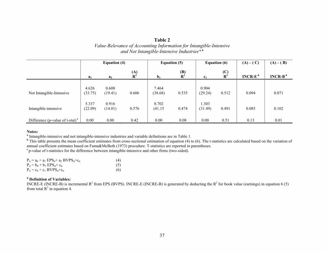
Table 2 reports the mean coefficient estimates from the above price regressions in

equations (4-6). The first three columns report the estimation results of full model,

equation (4). The mean coefficient estimate for EPS for intangible intensive industries is

5.337, while it is 4.626 for not intangible-intensive industries. The difference in

coefficient estimates is statistically significant (p-value of the difference <0.01). There is

even greater difference in the coefficient estimates for BVPS, which is 0.916, for

intangible-intensive industries and 0.608, for not intangible-intensive (p-value of the

difference <0.01). Moreover, there is not a statistically significant difference in R2

between intangible-intensive and not intangible-intensive industries. The R2 is 0.576 for

intangible-intensive industries, while it is 0.606 for not intangible-intensives. These

results are consistent which CMW.4

The next two columns report the mean coefficient estimates of equation (5),

where we include only EPS in the regression. Consistent with CMW, the R2s for both

groups are lower compared to the full model in equation (4); they are 47.4% and 53.3%

for intangible-intensive and not intangible-intensive industries, respectively and the

difference between two groups is around 6%, which is marginally significant (p-value of

the difference = 0.08). The next two columns report the mean coefficient estimates for

equation (6). The R2 for intangible-intensive industries is 50.1%, while it is 51.2% for not

intangible-intensive industries. The difference between both groups is 1.1%, much

smaller compared to the regression with EPS only in equation (5). Incremental R2 from

earnings is 9.40%, greater than that for book value for not intangible-intensive industries.

4 In Table 4 CMW report that the R2 is 50-51% in the period between 1953 to 1972, while it is around 60-75% in period between 1972 and 1993. This is consistent with their main results that value-relevance of accounting information is increasing over time.

21

However, the oppositve is true for intangible intensive industries (i.e. Incremental R2

from earnings is 8.5%, lower than 10.20%, for book value for intangible-intensive).

Overall, Table 2 is consistent with CMW that there is not an economically significant

difference in value-relevance of accounting information between intangible-intensive

than not intangible-intensive industries.

Table 3 presents the results of price regressions in equations (4-6) using adjusted

book values and earnings under hypothetical capitalization of earnings. Neither R2, nor

the coefficient estimates of EPSAJ and BVPSAJ in equation (4�’) is much different than

those with unadjusted numbers in Table 2. However, The R2 in EPSAJ only regression in

equation (5�’) for intangible-intensive increases to 51.10% compared to that of 47.40% in

Table 2 (In untabulated results we find that increase in R2 is marginally significant). On

the other hand, there is not much change in the R2 for not intangible-intensive firms

compared to those in Table 2. Hence adjusting earnings makes an economically

significant increase in the R2 for only intangible-intensive firms. There is also only 0.50-

0.70 increase in the R2 for BVPSAJ only regression in equation (6�’) suggesting that

adjusting book value for expensing of R&D does not make much improvement in value-

relevance for both groups. The last two columns show the impact of adjustment on the

incremental R2 for earnings and book values. While there is not much change in the

incremental R2 from earnings, the incremental R2 from book value declines significantly

for intangible-intensive industries (i.e. it is 7.10% in table 3 after adjustment versus

10.20% in Table 2 before adjustment; a 30% decline). In fact, the incremental R2 from

earnings after adjustment exceeds that from book value for intangible-intensive industries

while opposite was true before the adjustment. The adjustment of earnings and book

values does not lead to much increase in total R2 suggesting that the decline in

22

incremental R2 from book value is substituted by increase in R2 common to earnings and

book value. To further investigate the impact of distortion in accounting numbers in

value-relevance, in untabulated analysis, we divide intangible-intensive industries into

four groups, high and low based on the distortion in earnings and also high and low

groups based on distortion in book value. We estimate equation (4) to see how the R2

varies across the groups. We find that R2 is the lowest in the group with high distortion

and high book value per share (i.e. the R2 for high, high group was 38%, almost 20%

lower than that in Table 2). Moreover, we find that, consistent with Table 3, the distortion

in EPS is much stronger in affecting value-relevance than distortion in BVPS.

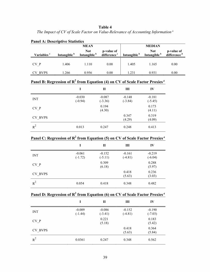
5.3. The Impact of Scale Factor on Value-Relevance

In this Section we investigate whether there are any systematic difference in scale

factor between intangible-intensive and not intangible-intensive industries which might

affect the value-relevance of accounting information documented in Table 2. Consistent

with Brown et al. (1999), we use book value per share, BVPS, and share price, P as

proxies for scale factor. Panel A of Table 4 presents the mean and median for CV of scale

factor proxies. The mean value of CV_P, the CV of share price is 1.408, while it is 1.110

for not intangible-intensive industries, which suggests a 27% (=(1.408-1.110)/1.110)

difference between two groups. The mean value of CV_BVPS, CV of book value per

share for intangible industries is 1.294, while it is 0.964 for not intangible-intensive

industries, again suggesting that CV of BVPS is 32% (=(1.294-0.964)/0.964) larger for

intangible-intensive industries. The differences in CV of scale factor proxies raise

possibility that the primary reason for high R2 for intangible-intensive industries

documented in Table 2 might be lack of control for scale factor.

23

The estimation results of equation (7) where dependent variable is R2 from the

full model are in Panel B of Table 4. When we do not include the CV of scale factor

proxies, there is only 3.0% difference between intangible intensive and not intangible-

intensive firms and the difference is not statistically significant. We include in the

regression only one scale factor proxy at a time to see the impact of each one separately.

First, we only include CV of share price, CV_P. The coefficient estimate of INT is -0.087

(p-value<0.01). The next column shows the estimation results when we include only

CV_BVPS. The coefficient estimate of INT is -0.148 (p-value<0.01), larger than the

estimation with CV_P. The last column shows the estimation results of equation (7). The

coefficient estimate of INT is -0.181 (p-value<0.01), larger than the estimation results

with any of CVs alone, suggesting that each of the scale factor proxy has incremental

explanatory power. Given that the R2 for not intangible-intensive firms reported in Table

2 is around 60%, the value-relevance of combined earnings and book values is 30%

lower for intangible-intensive than not intangible-intensive industries after controlling for

scale factor proxies (=18% / 60%). Overall, the results in panel B of Table 4 suggest that

the discrepancy between Amir and Lev (1996) and CMW is due to correlated omitted

variable in the form of scale factor. Panel C presents the results when the dependent

variable is R2 generated from EPS alone regression in equation (5). The coefficient

estimate of INT increases from -6.10% to -21.90%, when we control CV scale factor.

Hence, the largest difference in R2 between intangible-intensive and not-intangible-

intensive industries is realized for EPS alone regression. Panel D reports the results when

the dependent variable is R2 from equation (6) where the BVPS alone is the regressor.

The coefficient estimate of INT increases from -0.90% to -19.0%, when we control CV

scale factor.

24

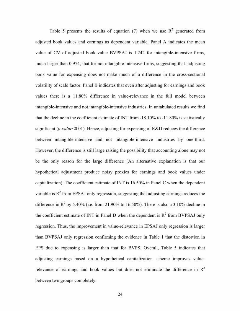
Table 5 presents the results of equation (7) when we use R2 generated from

adjusted book values and earnings as dependent variable. Panel A indicates the mean

value of CV of adjusted book value BVPSAJ is 1.242 for intangible-intensive firms,

much larger than 0.974, that for not intangible-intensive firms, suggesting that adjusting

book value for expensing does not make much of a difference in the cross-sectional

volatility of scale factor. Panel B indicates that even after adjusting for earnings and book

values there is a 11.80% difference in value-relevance in the full model between

intangible-intensive and not intangible-intensive industries. In untabulated results we find

that the decline in the coefficient estimate of INT from -18.10% to -11.80% is statistically

significant (p-value<0.01). Hence, adjusting for expensing of R&D reduces the difference

between intangible-intensive and not intangible-intensive industries by one-third.

However, the difference is still large raising the possibility that accounting alone may not

be the only reason for the large difference (An alternative explanation is that our

hypothetical adjustment produce noisy proxies for earnings and book values under

capitalization). The coefficient estimate of INT is 16.50% in Panel C when the dependent

variable is R2 from EPSAJ only regression, suggesting that adjusting earnings reduces the

difference in R2 by 5.40% (i.e. from 21.90% to 16.50%). There is also a 3.10% decline in

the coefficient estimate of INT in Panel D when the dependent is R2 from BVPSAJ only

regression. Thus, the improvement in value-relevance in EPSAJ only regression is larger

than BVPSAJ only regression confirming the evidence in Table 1 that the distortion in

EPS due to expensing is larger than that for BVPS. Overall, Table 5 indicates that

adjusting earnings based on a hypothetical capitalization scheme improves value-

relevance of earnings and book values but does not eliminate the difference in R2

between two groups completely.

25

5.4. Intertemporal Pattern in Value-Relevance

The results of intertemporal regression of equation (8) and (9) are in Table 6.

Panel A shows the results when the dependent variable is total R2 from the full model.

The first column shows the estimation of equation (8) where we do not separate the

industries into intangible-intensive and not-intangible-intensive groups. The coefficient

estimate of TIME is -0.005 negative and significant (p-value<0.01). This result is

consistent with Brown et al. (1999), which documents a decline in value-relevance for the

period of 1958-1996. The magnitude of decline is greater compared to Brown et al.,

probably because we are covering the period after 1975.5 The next column shows the

coefficient estimates of equation (9) without control variables. The coefficient estimate of

TIME is -0.002, statistically insignificant, suggesting that there is not a statistically

significant decline in value-relevance for not intangible-intensive industries. The

coefficient estimate of INT*TIME is -0.006 (p-value<0.01), suggesting that the decline in

value-relevance for intangible intensive industries is 6 basis points greater than not

intangible-intensive. The last two columns show the estimation results of equation (9).

The coefficient estimate of TIME is -0.002, statistically insignificant, and INT*TIME is -

0.007 (p-value<0.01), suggesting that including CV of scale factor proxies slightly

increases the magnitude of decline in value-relevance for intangible-intensive industries.

Moreover, the sum of the coefficients TIME and INT*TIME is -0.009 (p-value<0.01),

which confirms that there is a statistically significant decline in value-relevance for

intangible-intensive industries. Overall, Panel A of Table 6 indicates that there is not a

statistically significant decline in value-relevance for not intangible-intensive industries

5 As shown in Brown et al. (1999) Figure 3(a), the total R2 from the full model is lower in the period before 1975. However, when we repeat our analysis using the sample period of 1958-1996, the slope coefficient in our estimation for all industries is -0.003, similar to show reported in Brown et al (1999).

26

and that the decline documented by Brown et al. (1999) for all industries is primarily

driven by intangible-intensive industries. CMW document that R2 from full model in

equation (4) is attenuated when we account for one-time items, size and losses. In table 1,

we show that the frequency of losses is greater; market value of equity is larger and one-

time items are larger in absolute magnitude for intangible-intensive industries than those

for not intangible-intensive, indicating that the intertemporal pattern in value relevance

largely is affected by intangible-intensive industries.

Panel B documents intertemporal pattern in incremental R2 from EPS. There is no

statistically significant intertemporal trend for all industries.6 However, when we separate

the industries into intangible-intensive and not, we find that there is a statistically

significant decline in incremental R2 from EPS for intangible-intensive industries, while

there is no statistically significant trend for not intangible-intensive industries. Dichev

and Tang (2008) documents a decline in matching of revenues and expenses and argue

that intertemporal decline in value-relevance of earnings documented by CMW might be

due to intertemporal decline in matching. Given that expensing of R&D leads to decline

in matching, the results here are consistent with Dichev and Tang�’s conjecture that

decline in value relevance of earnings might be due to increase in mismatching probably

due to intangible-intensive industries.

Panel C reports the intertemporal pattern in incremental R2 from BVPS. There is

an intertemporal increase for all industries as reported in the first column. However,

when we separate industries into intangible-intensive and not, we see that the increase is

6 CMW documents a decline in the incremental R2 from earnings. However, their estimation period starts at 1953. Incremental R2 from earnings is quite high in 1950s and 1960s ; start to decline after 1963 and becomes quite low in mid 1970s. Hence different results documented here is due to different sample periods. In fact they also show in their Figure 1(a) that in the period between 1975 and 1993, the incremental R2 is quite flat.

27

0.4% larger (i.e. the increase for intangible-intensive firms is 0.1+0.4=0.5) for intangible-

intensive industries. Moreover, when we control for CV of scale factor proxies, there is

not statistically significant increase for not intangible-intensive industries. Overall, Panel

B and C suggest that the intertemporal pattern in the incremental R2 from earnings and

book values in CMW is realized primarily in intangible-intensive industries, while there

is not statistically significant trend for not intangible intensive industries.

5.5. Robustness Checks

We also perform several robustness checks. In untabulated results we also run

equation (7) for high and low R&D intensity firms. More specifically, we drop non-R&D

firms from the estimation. Low R&D intensity firms are those in the first three quartiles

of R&D capital to assets ratio and high R&D intensity firms are those in the top. We find

that the difference in R2 from price regressions between high and low R&D groups is

3.90%, statistically insignificant, (p-value=0.22) without controlling CV of scale factor

proxies. However, when we include the CV of scale factor proxies, the difference

between high and low R&D groups becomes 20%, statistically significant at 1% level.

These results suggest that when we define intangible-intensity based on R&D intensity,

the results are similar.

In addition, we include additional control variables in the estimation of equation

(7). CMW suggest that the intertemporal increase in value-relevance of accounting

information is due to increase in frequency of extraordinary items, proportion of the firms

that report losses and decline in average inflation adjusted market value of equity over

time. We augment equation (7) by adding ONE, the mean value of absolute value of one-

time items as a percentage of core net earnings in year t, LOSS, the percentage of firms

28

that have core net income less than zero in year t and SIZE, the natural log of mean

inflation-adjusted market value of equity of firms in year t. We find that both INT in

equation (7) is still negative and statistically significant at 1% level, suggesting that the

differential value-relevance for intangible-intensive industries is not eliminated with the

inclusion of these variables.

6. Conclusion and Future Research

Prior research suggests that accounting information is not useful when valuing firms

with large amount of intangibles (Amir and Lev, 1996). However, CMW find that value-

relevance for intangible-intensive is as high as not intangible-intensive industries. An

explanation for this discrepancy is that the high value relevance for intangible-intensive

industries documented by CMW is due to lack of control for scale factor (Brown et al.,

1999). We find that once we control for CV of scale factor, the value-relevance for

intangibles-intensive industries is substantially lower than not intangible-intensive

industries. In addition, adjusting earnings and book values for expensing of R&D reduces

the difference in value-relevance between intangible-intensive and not intangible-

intensive industries by one-third but does not completely eliminate it. Moreover, we find

that adjusting earnings has greater impact on value-relevance of earnings than book value

consistent with greater distortion in earnings. We also find that the decline in value-

relevance for all firms documented by Brown et al. (1999) is due to intangible-intensive

industries while there is no such decline for not intangible-intensive.

An extension of this study might investigate what are the underlying reasons for

higher variability of scale factor among intangible-intensive industries. Several reasons

for high variability of scale factor might be size differences, more volatile operating

29

performance and greater mismatching of revenues and expenses among intangible-

intensive industries than others. Another venue for future research is to investigate factors

that affect value-relevance when using return regressions. Return regressions are free of

scale, hence scale might not be the omitted variable causing high value-relevance in

return regressions. However, intangible-intensive firms have higher growth opportunities

which might affect the value-relevance in return regressions for these firms.

30

References Amir, E., B. Lev. 1996. �“Value-relevance of nonfinancial information: The wireless communications industry.�” Journal of Accounting and Economics, 22: 3-30.

Brown, S. K. Lo, T Lys. 1999. �“Use of R2 in accounting research: measuring changes in value relevance over the last four decades.�” Journal of Accounting and Economics, 28: 83-115.

Chan, L, J. Lakonishok, T. Sougiannis. 2001. �“The stock market valuation of research and development expenditures.�” Journal of Finance, 56: 2,431-2,457.

Collins, D.W., S.P. Kothari. 1989. �“An analysis of intertemporal and cross-sectional determinants of earnings-response-coefficients.�” Journal of Accounting & Economics, 11: 143�–181.

Collins, D.W., E.L. Maydew, I.S. Weiss. 1997. �“Changes-in the value-relevance of earnings and book values over the past forty years.�” Journal of Accounting and Economics, 24: 39-67.

Core, J.E. W.R. Guay, A. Vand Buskirk. 2003. �“Market valuations in the New Economy: an investigation of what has changed.�” Journal of Accounting and Economics, 34: 43-67.

Darrough, M.N., J. Ye. 2007 “Valuation of Loss Firms in a Knowledge-Based Economy.�” Review of Accounting Studies, 12:61-93.

Dichev, I.L. and V.W. Tang. 2008. �“Matching and the changing properties of accounting earnings over the last 40 years.�” Accounting Review, 83:1460-1425.

Elliot, J., J. Hanna. 1996. �“Repeated accounting write-offs and the information content of earnings.�” Journal of Accounting Research, 34:135-155.

Fama, E.F., J. MacBeth. 1973 �“Risk, return and equilibrium: Empirical tests.�” Journal of Political Economy, 81:607-636.

Francis, J., K. Schipper. 1999. �“Have financial statements lost their relevance?�” Journal of Accounting Research, 37:319-352.

Franzen, A.L., K.J. Rodgers, T.T. Simin. 2007. �“Measuring distress risk: The effect of R&D intensity.�” Journal of Finance, 62: 2,931-2968.

Hayn, C. 1995. �“The information content of losses.�” Journal of Accounting and Economics, 20:125-153.

Kothari, S.P., T.E. Laguerre, J.A. Leone. 2002. �“Capitalization versus expensing: Evidence on the uncertainty of future earnings from capital expenditures versus R&D outlays.�” Review of Accounting Studies, 7: 355-382.

Lev B. 2001. �“Intangibles�” Brookings Institution Press, Washington D.C.

31

Lev, B., T. Sougiannis. 1996. �“The capitalization, amortization and value-relevance of R&D.�” Journal of Accounting and Economics, 21: 107-138.

Lev, B., P. Zarowin. 1999. �“The boundaries of financial reporting and how to extend them.�” Journal of Accounting Research, 37:353-385.

Monahan S. 2005. �“Conservatism, growth and the role of accounting numbers in the fundamental analysis process.�” Review of Accounting Studies, 10: 227-260.

32

Figure 1a Median Value of R&D Expense to Asset Ratio across Time for Intangible-Intensive Industries

0

0.01

0.02

0.03

0.04

0.05

0.06

0.07

0.08

1975

1977

1979

1981

1983

1985

1987

1989

1991

1993

1995

1997

1999

2001

2003

2005

Figure 1b Median Value of R&D Capital to Asset Ratio across Time for Intangible-Intensive Industries

0

0.02

0.04

0.06

0.08

0.1

0.12

0.14

0.16

0.18

0.2

1975

1977

1979

1981

1983

1985

1987

1989

1991

1993

1995

1997

1999

2001

2003

2005

33

Figure 2a Median Value of Distortion in EPS across Time for Intangible-Intensive and Not Intangible-Intensive Industries. Distortion in EPS = [(EPS_adj �– EPS)/abs(EPS)]

Figure 2b Median Value of Distortion in BVPS across Time for Intangible-Intensive and Not Intangible-Intensive Industries. Distortion in BVPS = [(BVPS_adj �– BVPS)/BVPS]

34

Figure 3 The R2 for Annual Regressions of Price on Book Value and Earnings for

Intangible-Intensive and Not Intangible-Intensive Industries

35

Table 1 Descriptive Statistics for Intangible-Intensive

and Not Intangible-Intensive Industries a, b Panel A: Descriptive Statistics (N=152,871) MEAN MEDIAN

Variables e Intangible Not

Intangible p-value of

difference c Intangible Not

Intangible p-value of

difference d

P 14.815 17.211 0.00 8.710 13.375 0.00

EPS 0.362 1.193 0.00 0.143 0.823 0.00

EPSAJ 0.585 1.252 0.00 0.251 0.869 0.00

BVPS 6.118 11.583 0.00 3.683 8.364 0.00

BVPSAJ 7.372 12.123 0.00 4.656 8.788 0.00

RDAS 0.103 0.018 0.00 0.048 0.000 0.00

RDCAPS 0.250 0.044 0.00 0.105 0.000 0.00

ONE -0.079 -0.052 0.00 0.000 0.000 0.00

LOSS 0.392 0.193 0.00 0.000 0.000 0.00

MV 1,733 1,149 0.00 100 99 0.60

ONEP 0.319 0.240 0.00 0.000 0.000 0.00 Notes: a The sample consists of firm-year observation in CRSP and Compustat between 1975 and 2006 with book value of equity and total assets greater than zero. We exclude the observation at top and bottom ranked at 1.5% of earnings-to-price, book-value-to-market value, absolute value of one-time items as a percent of net income before one-time items and (3) observations with studentized residuals greater than four in any of the yearly regressions of price on earnings, price on book value, price on earnings and book value. Intangible-intensive industries contain 33,493 firm-year observations, while there are 119,378 firm-year observations for not intangible-intensive industries. b Intangible industries are SIC codes 282 plastic and synthetic materials; 283 drugs; 357 computer and office equipment; 367 electronic components and accessories; 48 communications; 73 business services; 87 engineering, accounting, R&D and management services. The rest of industries are included in not intangible-intensive group. c p-value of t-statistics for the difference between intangible-intensive and other firms (two-sided). d p-value of z-stat based on Wilcoxon rank sum test for the difference between intangible-intensive and other firms (two-sided). e Definition of Variables: P is share price three month after year-end in year t adjusted for stock splits. EPS is earnings per share of in year t calculated as Net Income (NI) divided by the number of shares outstanding (CSHO from Compustat). BVPS Book value per share in year t calculated as book value of equity (CEQ from Compustat) divided by

36

the number of shares outstanding. RDAS is R&D expense (XRD from Compustat) to total asset (AT from Comupstat) ratio. RDCAPS is R&D capital to total asset ratio. ONE is one-time items per share calculated as one-time items (i.e. sum of extraordinary items (XI from Compustat), discontinued operations (DISC from Compustat) and special items (SPI from Compustat)) divided by the number of shares outstanding. LOSS is frequency of loss. A firm is considerd to be a loss firm if core earnings (net income (NI from Compustat) minus one-time items) is less than zero. MV is market value of equity; calculated as share price times shares outstanding three months after fiscal year end both from CRSP. ONEP is absolute value of one-time items as a percentage of core earnings.

37

Table 2 Value-Relevance of Accounting Information for Intangible-Intensive

and Not Intangible-Intensive Industries a, b

Equation (4) Equation (5) Equation (6) (A) – ( C) (A) – ( B)

a1 a2 (A) R2 b1

(B) R2 c1

(C) R2 INCR-E d INCR-B d

Not Intangible-Intensive 4.626

(33.75) 0.608

(19.41) 0.606 7.464

(38.68) 0.535 0.904

(29.24) 0.512 0.094 0.071

Intangible-intensive 5.337

(22.09) 0.916

(14.01) 0.576 8.702 (41.15 0.474

1.303 (31.49) 0.491 0.085 0.102

Difference (p-value of t-stat) c 0.00 0.00 0.42 0.00 0.08 0.00 0.51 0.13 0.01 Notes: a Intangible-intensive and not intangible-intensive industries and variable definitions are in Table 1. b This table presents the mean coefficient estimates from cross-sectional estimation of equation (4) to (6). The t-statistics are calculated based on the variation of annual coefficient estimates based on Fama&McBeth (1973) procedure. T-statistics are reported in parentheses. c p-value of t-statistics for the difference between intangible-intensive and other firms (two-sided). Pit = a0 + a1 EPSit+ a2 BVPSit+ it (4) Pit = b0 + b1 EPSit+ it (5) Pit = c0 + c1 BVPSit+ it (6) d Definition of Variables: INCRE-E (INCRE-B) is incremental R2 from EPS (BVPS). INCRE-E (INCRE-B) is generated by deducting the R2 for book value (earnings) in equation 6 (5) from total R2 in equation 4.

38

Table 3 Value-Relevance of Accounting Information with Adjusted Earnings and Book Values a, b

Equation (4’) Equation (5’) Equation (6’) (A) – ( C) (A) – ( B)

a1 a2 (A) R2 b1

(B) R2 c1

(C) R2 INCR-E d INCR-B d

Not Intangible-Intensive 4.522

(33.39) 0.591

(18.73) 0.613 7.340

(34.18) 0.541 1.088

(28.34) 0.519 0.094 0.072

Intangible-intensive 0.582 8.345

(46.39) 0.511 1.300

(31.18) 0.496 0.086 0.071

Difference (p-value of t-stat) c 0.00 0.00 0.00 0.00 0.17 0.85 Notes: a Intangible-intensive and not intangible-intensive industries and variable definitions are in Table 1. b This table presents the mean coefficient estimates from cross-sectional estimation of equation (4�’) to (6�’). The t-statistics are calculated based on the variation of annual coefficient estimates based on Fama&McBeth (1973) procedure. T-statistics are reported in parentheses. c p-value of t-statistics for the difference between intangible-intensive and other firms (two-sided). Pit = a0 + a1 EPSAJit+ a2 BVPSAJit+ it (4�’) Pit = b0 + b1 EPSAJit+ it (5�’) Pit = c0 + c1 BVPSAJit+ it (6�’)

d Definition of Variables: INCRE-E (INCRE-B) is incremental R2 from EPS (BVPS). INCRE-E (INCRE-B) is generated by deducting the R2 for book value (earnings) in equation 6 �‘(5�’) from total R2 in equation 4.

39

Table 4 The Impact of CV of Scale Factor on Value-Relevance of Accounting Information e

Panel A: Descriptive Statistics MEAN MEDIAN

Variables e Intangible b Not

Intangible b p-value of difference c Intangible b

Not Intangible b

p-value of difference d

CV_P 1.406 1.110 0.00 1.405 1.165 0.00

CV_BVPS 1.266 0.956 0.00 1.231 0.931 0.00 Panel B: Regression of R2 from Equation (4) on CV of Scale Factor Proxies d

I II III IV

INT -0.030 (-0.94)

-0.087 (-3.36)

-0.148 (-3.84)

-0.181 (-5.45)

CV_P 0.194 (4.30) 0.173

(4.11)

CV_BVPS 0.347 (4.29)

0.319 (4.09)

R2 0.013 0.247 0.248 0.413

Panel C: Regression of R2 from Equation (5) on CV of Scale Factor Proxies d

I II III IV

INT -0.061 (-1.72)

-0.152 (-5.11)

-0.161 (-4.81)

-0.219 (-6.04)

CV_P 0.309 (6.18) 0.288

(5.97)

CV_BVPS 0.418 (5.63)

0.236 (3.03)

R2 0.054 0.418 0.348 0.482

Panel D: Regression of R2 from Equation (6) on CV of Scale Factor Proxies d

I II III IV

INT -0.009 (-1.44)

-0.086 (-3.41)

-0.152 (-4.81)

-0.190 (-7.03)

CV_P 0.221 (5.18) 0.183

(5.42)

CV_BVPS 0.418 (5.63)

0.364 (5.84)

R2 0.0361 0.247 0.348 0.562

40

Notes: a Intangible-intensive and not intangible-intensive industries are defined in Table 1. b p-value of t-statistics for the difference between intangible-intensive and other firms (two-sided). c p-value of z-stat based on Wilcoxon rank sum test for the difference between intangible-intensive and other firms (two-sided). d This table presents the mean coefficient estimates from equation (7). T-statistics are reported in parentheses. R2

pt = 0 + 1 INTpt+ 2 CV_Ppt+ 3 CV_BVPSpt+ pt (7) e Definition of Variables: R2

pt is R2 from estimation of equation (4), (5) or (6) for group p in year t (there are two groups: intangible-intensive and not intangible-intensive).

INT pt is an indicator variable which equals one for intangible-intensive group and zero for not intangible-intensive. The industries in intangible-intensive group as defined as by CMW Not intangible-industries are all industries except intangible-intensive industries.

CV_Ppt is coefficient of variation of share price for group p in year t (it is calculated as standard deviation of share price divided by absolute value of mean).

CV_BVPSpt is coefficient of variation for book value per share for group p in year t (it is calculated as standard deviation of book value per share divided by mean).

41

Table 5 The Impact of CV of Scale Factor Proxies on Value-Relevance of Accounting Information

with Adjusted Earnings and Book Values e Panel A: Descriptive Statistics MEAN MEDIAN

Variables e Intangible b Not

Intangible b p-value of difference c Intangible b

Not Intangible b

p-value of difference d

CV_BVPSAJ 1.242 0.974 0.00 1.201 0.969 0.00 Panel B: Regression of R2 from Equation (4’) on CV of Scale Factor Proxies d

I II III IV

INT -0.012 (-0.39)

-0.061 (-2.39)

-0.102 (-3.64)

-0.118 (-4.47)

CV_P 0.167 (3.85) 0.114

(2.79)

CV_BVPSAJ 0.334 (4.91)

0.276 (4.01)

R2 0.004 0.199 0.286 0.368

Panel C: Regression of R2 from Equation (5’) on CV of Scale Factor Proxies d

I II III IV

INT -0.030 (-0.89)

-0.111 (-3.89)

-0.135 (-3.82)

-0.165 (-5.41)

CV_P 0.277 (5.74) 0.225

(4.79)

CV_BVPSAJ 0.390 (4.51)

0.270 (3.55)

R2 0.016 0.361 0.262 0.467

Panel D: Regression of R2 from Equation (6’) on CV of Scale Factor Proxies d

I II III IV

INT -0.024 (-0.80)

-0.089 (-3.70)

-0.135 (-5.21)

-0.159 (-6.89)

CV_P 0.224 (5.52) 0.161

(4.62)

CV_BVPSAJ 0.416 (6.56)

0.330 (5.70)

R2 0.014 0.343 0.422 0.574

42

Notes: a Intangible-intensive and not intangible-intensive industries are defined in Table 1. b p-value of t-statistics for the difference between intangible-intensive and other firms (two-sided). c p-value of z-stat based on Wilcoxon rank sum test for the difference between intangible-intensive and other firms (two-sided). d This table presents the mean coefficient estimates from equation (7). T-statistics are reported in parentheses. R2

pt = 0 + 1 INTpt+ 2 CV_Ppt+ 3 CV_BVPSAJpt+ pt (7�’) e Definition of Variables: R2

pt is R2 from estimation of equation (4�’), (5�’) or (6�’) for group p in year t (there are two groups: intangible-intensive and not intangible-intensive).



CV_BVPSAJpt is coefficient of variation for adjusted book value per share for group p in year t (it is calculated as standard deviation of book value per share divided by mean).

43

Table 6 The Intertemporal Pattern in Value-Relevance of Accounting Information for Intangible-

Intensive and Not Intangible-Intensive Industries a, b Panel A: Intertemporal Pattern in Total R2 from Equation (4)

Variables d Equation (8) Equation (9)

without control Equation (9)

TIME -0.005 (-2.97)

-0.002 (-1.17)

-0.002 (-0.96)

INT 0.060 (1.48)

-0.014 (-0.24)

INT * TIME -0.006 (-2.65)

-0.007 (-3.07)

CV_P -0.095 (-1.36)

-0.033 (-0.35)

CV_BVPS 0.181 (2.78)

0.314 (4.40)

R2 0.2801 0.321 0.492 d F-test: TIME + INT * TIME = 0 24.69**

13.44**

Panel B: Intertemporal Pattern in Incremental R2 from EPS

Variables d Equation (8) Equation (9) w/o control Equation (9)

TIME -0.001 (-0.74)

0.001 (1.71)

0.000 (0.09)

INT 0.006 (0.48)

0.046 (2.48)

INT * TIME -0.001 (-1.79)

-0.002 (-2.20)

CV_P -0.003 (-0.23)

-0.045 (-1.58)

CV_BVPS 0.049 (2.55)

0.065 (-2.89)

R2 0.181 0.119 0.264 d F-test: TIME + INT * TIME = 0 0.06 2.61*

44

Panel C: Intertemporal Pattern in Incremental R2 from BVPS

Variables d Equation (8) Equation (9) w/o control Equation (9)

TIME 0.002 (2.71)

0.001 (2.28)

0.001 (1.48)

INT -0.003 (-1.68)

-0.043 (-1.76)

INT * TIME 0.004 (4.26)

0.004 (3.87)

CV_P -0.102 (-1.78)

-0.045 (-1.58)

CV_BVPS 0.136 (3.50)

0.065 (-2.89)

R2 0.489 0.604 0.6293 d F-test: TIME + INT * TIME = 0 70.64** 16.28**

Notes: a Intangible-intensive and not intangible-intensive industries are defined in Table 1. b This table presents the coefficient estimates from equations (8) and (9). T-statistics are reported in parentheses. R2

t = 0 + 1 TIMEt+ 2 CV_EPSt+ 3 CV_BVPSt+ t (8) R2

pt = 0 + 1TIMEpt + 2INTpt+ 3INTpt*TIMEpt + 4CV_EPSpt+ 5CV_BVPSpt+ pt (9) c F-test results show whether the sum of coefficient estimates of TIMEpt + INTpt*TIMEpt equals zero in equation (9). * and ** shows statistical significance at 10% and 5% respectively, with the F-test.

d Definition of Variables: TIMEpt is year t minus 1975 for group p. R2

pt is either R2 from estimation of equation (4) or incremental R2 for EPS and BVPS for group p in year t (there are two groups: intangible-intensive and not intangible-intensive).



CV_BVPSpt is coefficient of variation for book value per share for group p in year t (it is calculated as standard deviation of book value per share divided by mean).

Value-Relevance of Accounting Information for Intangible...

Documents

Transcript of Value-Relevance of Accounting Information for Intangible...