Sampan Nettayanun*

Value Investing: Circle of Competencein the Thai Insurance Industry

DOI 10.1515/apjri-2016-0019

Abstract: This study explores the strategy of value investing, specifically for theinsurance industry in Thailand. It employs multiple measures of “value,” sui-table for insurance companies, such as the price-to-earning (PE), price-to-book(PB), and cyclically adjusted price-to-earnings (CAPE). Value premium exists inthe Thai insurance industry, and most of the value portfolios constructed fromthese measures significantly outperform the market, even when adjusting forprice volatility and portfolio’s β. The cumulative returns are also higher for thevalue stocks, when compared to the growth stocks, and the Thai stock market.Constructing a value portfolio, using the PE ratio, results in the highest returnsand is far better than PB and CAPE. The value anomaly cannot be fullyexplained by either the capital asset pricing model or the Fama-French three-factor models.

Keywords: value investing, portfolio management, circle of competence, riskmanagement, insurance, property & casualty insurance, life insurance

1 Introduction

Value investing has been popular among institutional and individual investors inThailand. The idea is originally from Dodd and Graham (1951) and Graham (2003).Various studies, such as Basu (1977), Fama and French (1992, 1993, 1996, 1998,2006, 2012, 2015), Piotroski (2000), Piotroski and So (2012), Asness, Moskowitz,and Pedersen (2013), Asness et al. (2015), and Novy-Marx (2013, 2015), find thatvalue portfolios outperform growth portfolios. Value stocks are defined as eitherhaving a low price-to-book ratio, or a low price-to-earnings ratio. Growth stocksare defined as either having a high PB ratio, or a high PE ratio.

This study puts a new twist on the value investing research. The objectiveis to focus exclusively on value portfolios constructed using only insurance

*Corresponding author: Sampan Nettayanun, Department of Business, Economics andCommunications, Naresuan University, 99 Moo 9 Taphoe, Phitsanulok, Mueng 65000, Thailand,E-mail: sampann@nu.ac.th

Asia Pac J Risk Insur 2016; aop

companies. The idea of investing in a particular set of stocks that each investorknows well is well established in the value investing community. This philoso-phy is called the investor’s “circle of competence”. To the author’s knowledge,this study is the first to formally explore the circle of competence. It also aims tofind the best value measure for insurance companies to quantitatively constructa value portfolio. Finally, it intends to explain the value anomaly using existingtheoretical and empirical models similar to previous literature.

Notable value investors claim that the value investor does not have to knowor understand every company in the market. Investors might be able to imple-ment value investing using some companies or industries that they truly under-stand. The notion of a circle of competence has been popularized by WarrenBuffett and Charlie Munger, two of the most successful value investors. Theystate that they do not need to invest in companies or industries that they donot understand. For example, in a 1996 letter to shareholders of BerkshireHathaway, Buffett stated:

Should you choose, however, to construct your own portfolio, there are a few thoughtsworth remembering. Intelligent investing is not complex, though that is far from sayingthat it is easy. What an investor needs is the ability to correctly evaluate selected busi-nesses. Note that word ‘selected’: You don’t have to be an expert on every company, oreven many. You only have to be able to evaluate companies within your circle of compe-tence. The size of that circle is not very important; knowing its boundaries, however, isvital.1

In the same spirit as Warren Buffett, Andrew Carnegie, one of the world’swealthiest magnates also emphasized the importance of staying within the circleof competence by saying:

My advice to young men would be not only to concentrate their whole time andattention on the one business in life in which they engage, but to put every dollar oftheir capital into it. If there be any business that will not bear extension, the true policyis to invest the surplus in first-class security which will yield a moderate but certainrevenue if some other growing business cannot be found. As for myself my decision wastaken early. I would concentrate upon the manufacture of iron and steel and be masterin that.2

Is it true that by focusing on a particular industry, investors can beat themarket in the long term? This study explores the performance of value portfolioconstruction from stocks only in the Thai insurance industry using hand-collected

1 See the 1996 Warren Buffett’s Letter to Berkshire Shareholders of Berkshire Hathaway Inc.2 Carnegie (2012)

2 S. Nettayanun

data from the Stock Exchange of Thailand.3 This study is different from theprevious traditional value studies in the following ways. First, it studies valueinvesting in only a specific sector, namely the Thai insurance industry. By study-ing only one sector, it has the benefit of using a more proper and effective way toidentify value stocks. In addition, it eliminates heterogeneity among differentindustries when ranking stocks based on their value measures. As each sectorexperiences different growth prospects and cycles, and illustrates unlike charac-teristics, using a particular measure across all sectors seems to be inappropriateto identify value stocks. In addition, this study differentiates from other valuepremium studies because the insurance industry is a unique sector. The construc-tion of the balance sheet and the earnings statement are quite different from otherindustries. Therefore, the study needed to take a more careful approach whenanalyzing the value of investing in the insurance industry by offering variousmeasurements of value.

More specifically, price-to-book (PB) was used as a measure of value. Manyvalue investing gurus claim that it is the most appropriate way to measure theintrinsic value of an insurance company. As the balance sheet of an insurancecompany consists of financial assets and liabilities, the book value is theremainder of assets and liabilities that belong to equity owners. The PB mea-sure is similar to previous “value” studies. In addition, price-to-earnings (PE)ratio was used, similar to Basu (1977) to capture the value stocks. The cyclicallyadjusted price-to-earnings (CAPE) was also used, similar to Campbell andShiller (1988). This is due to the fact that the earnings of an insurance companyin a single year might affect the way we pick value stocks. For example, aninsurance company might have one particularly bad year, due to a catastrophicevent, and the event might create much lower earnings than the true earningpower of the company. The company might also be a good underwriter over along period of time. We can call this kind of company, “good but unlucky.”Therefore, this might result in a negative PE ratio for a catastrophic year. If weuse only a PE ratio to capture the value stock, some insurers might be

3 The author uses the SETSMART database provided by the Stock Exchange of Thailand. Thiseducational version is only available to some Thai universities for educational purposes. Theuniversities that have the Stock Exchange of Thailand Investment Center (SETIC), which is alearning center for investors, have the right to access the database. The database provides a lotof information for each stock. However, it is in a website style. For example, one page canprovide five-year balance sheet of a public company. The database does not provide financialinformation in a query-able structure like Compustat, CRISP, or NAIC databases. The author ofthis study, therefore, had to carefully collect insurers’ financial variables one-by-one at a time.This process is one of the most time-consuming tasks of this study.

Value Investing 3

eliminated from the analysis. Hence, average earnings might result in a moreappropriate measure of a value stock.

The results are in line with other studies. Constructing value portfoliosbased on PB, PE, and CAPE34 outperform both the market portfolios and thegrowth portfolios. However, using CAPE55 does not result in value premium. Inparticular, value investing greatly outperforms during the period between theAsian financial crisis and the global financial crisis. Adjusting for volatilityyields the same results. This implies that CAPM does not fully capture thevalue premium, similar to the results of Fama and French (2006). In addition,the Fama-French three-factor model does not capture the value anomaly. Thismight be due to the fact that the number of stocks in each portfolio is small.Therefore, the dispersion from non-systematic risks (the sample variance of εsis too high to be explained by the market returns). It dominates systematic riskwhich is represented by β. Therefore, there is no apparent relationship betweenthe returns of the value portfolio and the Fama-French factors. Overall, inves-tors can outperform the market, even adjusting for the volatility, by applying avalue investing strategy in the Thai insurance industry. However, investorsmust choose an appropriate value measure to construct the insurance valueportfolio.

This study proceeds as follows. Section 2 explores related theories andempirical findings about value investing. Section 3 outlines the portfolio con-struction procedures and how the data was collected. Section 4 reports theperformance of various portfolios when compared to the market. Section 5uses CAPM to explain the value anomaly in the Thai insurance industry.Section 6 attempts to explain the anomaly using the Fama-French three-factormodel. Lastly, the study concludes with a discussion of the implications of thefindings and recommendations for future research.

2 Related Theories and Empirical Findings

Benjamin Graham is the father of value investing. His books; Dodd andGraham (1951), and Graham (2003), propose a value strategy for investing.He states that investors can outperform the general market by constructing aportfolio consisting of a low price-to-book ratio or a low price-to-earnings ratio.

4 CAPE3 is cyclically adjusted price-to-earnings ratio based on three-year earnings.5 CAPE5 is cyclically adjusted price-to-earnings ratio based on five-year earnings.

4 S. Nettayanun

By using this strategy, investors have what Benjamin Graham calls margins ofsafety, which means that the price is below the intrinsic value of the business.Many prominent investors have successfully followed this unique strategy,such as Warren Buffett, Charlie Munger, Irvin Kahn, Walter Schloss, JoelGreenblatt, Christopher Browne, Seth Klarman, and Martin Whitman. Forinstance, Frazzini, Kabiller, and Pedersen (2013) find that BerkshireHathaway outperforms any stocks and mutual funds using Sharpe’s ratiocriteria. This is due to the combination of value, safe, quality investing, plusleverage. In addition to the success of the superinvestors from Graham-and-Doddsville,6 researchers also find evidence that value portfolios outperformmarket portfolios and growth portfolios.

Fama and French (1992, 1993, 1998, 2006, 2015) also discover that portfoliosof value stocks with a low PB, tend to outperform the market. There are doubtsthat the capital asset pricing model can capture the anomalies in the stockreturns. For example, Fama and French (2006) also find that value stocks out-perform the market, but CAPM does not capture the value premium. In additionto stocks, Asness, Moskowitz, and Pedersen (2013) find that value premiumexists through many other asset classes.

Focusing on the Thai stock market, Sareewiwatthana (2011, 2012, 2013),in line with Fama and French (1992, 1993, 1998, 2006, 2015), find that portfo-lios consisting of value stocks significantly outperform the market.Sareewiwatthana (2011) uses various measures, such as PB, PE, and dividendyield to pick value stocks. The study ranks them in order to form valueportfolios and defines the low PB, PE, and dividend yield to be value stocks.The study finds that value portfolios significantly outperformed the SET index.Sareewiwatthana (2012) combines growth and the price-to-earnings ratio toform a PEG ratio to capture the value stocks. The study constructs a portfoliowith a low PEG ratio and finds that it outperforms the market and also a low-PEG portfolio. Sareewiwatthana (2013) implements Sareewiwatthana (2012) byadding the other ratios, such as return of equity (ROE) and return on asset(ROA). Adding these ratios help value portfolios to outperform the market evenbetter. Overall, the evidence suggests that value investing outperforms themarket in the Stock Exchange of Thailand.

Value anomaly can be explained by both a rational and behavioralargument. According to the model in Sharpe (1964), higher (lower) risk stocksshould have a higher (lower) expected return. Value stocks occur because

6 Buffett, Warren (2004). “The Superinvestors of Graham-and-Doddsville.” Hermes: TheColumbia Business School Magazine: 415.

Value Investing 5

investors require higher than expected returns from riskier stocks. Therefore,the investors get higher than average returns due to the fact that they have tobear more risk in the portfolio. For example, Fama and French (1995) showthat lower PB stocks tend to be in a distressed situation and tend to provide alow return on equity. On the other hand, the behavioral finance literatureexplains that value stocks happen as a result of human behavior. For exam-ple, an overreaction by investors to news about a company can result in thestock prices being much lower than their fundamental value, according toBondt and Thaler (1985), Lakonishok, Shleifer, and Vishny (1994), and Daniel,Hirshleifer, and Subrahmanyam (1998). Noise traders and arbitrageurs canalso create the situation where the price and the fundamental value arediverged, according to Shleifer and Vishny (1997). A classic statement thatexplains the value premium from both schools of thought is from Dodd andGraham (1951):

In other words, the market is not a weighing machine, on which the value of each issue isrecorded by an exact and impersonal mechanism, in accordance with its specific qualities.Rather should we say that the market is a voting machine, whereon countless individualsregister choices which are the product partly of reason and partly of emotion.

This statement implies that value investing works because in the short term,stock prices can deviate from their fundamental value. However, over the longterm, the price can reflect the intrinsic value. The price can get to be very closeor at the true fundamental value. It is the job of value investors to find and getthe benefit of this anomaly by buying securities when the price and value aredeviated, and then waiting until the prices to go back to the intrinsic value in thelong term.

3 Portfolio Construction and Data Collection

This study uses the Stock Exchange of Thailand dataset from January of 1990until December of 2014, available from the SETSMART database. The StockExchange of Thailand (SET) has 521 companies listed in the stock market.The Stock Exchange of Thailand also has the Market for AlternativeInvestment (MAI) for smaller companies, with 129 companies.7 All Thai publiclylisted insurance companies are listed in the SET. Investors have no limit in

7 See http://www.set.or.th/set/marketstatistics.do

6 S. Nettayanun

investing in the Thai listed companies, although, foreign ownership is limited at49% for financial institutions in Thailand. The Thai insurance industry consistsof property and casualty (P&C), and life. According to the Office of InsuranceCommission of Thailand,8 the P&C insurance consists of four main lines ofbusinesses; fire, marine, auto, and miscellaneous. The life insurance industryconsists of life, accident, health, industrial life, and group life. Table 1 showsinformation for both the life and P&C insurance industry in Thailand. It includesnet premium written, total assets, number of insurers, number of insurers listedin the Stock Exchange of Thailand, and the number of stocks in the valueportfolio for each year.9

According to Table 1, there are some interesting findings. Firstly, the numberof insurers in the life insurance industry has been far less than the P&C insurers.Therefore, this might be a sign that the competition in the life insurance industrymight have been less aggressive than the P&C industry. In addition, the numberof both life and P&C jumped from 1996 to 1997. This was due to the fact that theBank of Thailand tried to make financial institutions more competitive, moreopen, and wanted to promote the insurance products for Thai people. Hence, theOffice of Insurance Commission of Thailand opened up for Thai and foreigninvestors to get new licenses to operate the life and P&C business. Manyobtained new licenses. However, the Asian financial crisis arrived right afterthe implementation of the new policy. The Office of Insurance Commission ofThailand stopped issuing new licenses, due to insolvency concerns. Therefore,the number of companies has not changed much for life insurers. On the otherhand, the number of P&C insurers has decreased from the peak of 80 to 64 dueto mergers and acquisitions, and insolvencies.

The net premium written for the life insurance industry has accelerated at ahigher rate than the P&C industry from 1997 to 2014. The author suspects thatThai people are more cautious about their financial planning. In addition, thefinancial planning has been popularized by life insurers, the Stock Exchange ofThailand, and also the Office of Insurance Commission of Thailand. It might alsobe because the life insurers have offered various new insurance products. The

8 See http://www.oic.or.th/th/industry/statistic/23. The data from 1997 to 2014 is available inelectronic version on the website. However, the data from 1990–1997 is only available on paper,which the author had to hand-collect from the library of the Office of Insurance Commission ofThailand. The Office of Insurance Commission of Thailand publishes the Annual InsuranceReport of Thailand every year that contains the information.9 The number of stocks in the value portfolio is derived from the methodology in the followingsections.

Value Investing 7

channels in which they have sold their product have increased tremendouslythrough their own networks, agents, brokers, and banks. The net premiumwritten and total assets in 2011–2012 for P&C increased significantly. This was

Table 1: Thai insurance industry information from 1990–2014.

Year Life NPW(in M Baht)

Life Assets(in M Baht)

# ofLife

P&C NPW(in M Baht)

P&C Assets(in M Baht)

# ofP&C

# ofStocks

# inPort

, , , ,

, , , ,

, , , ,

, , , ,

, , , ,

, , , ,

, , , ,

, , , ,

, , , ,

, , , ,

, , , ,

, , , ,

, , , ,

, , , ,

, , , ,

, , , ,

, , , ,

, , , ,

, , , ,

, , , ,

, ,, , ,

, ,, , ,

, ,, , ,

, ,, , ,

, ,, , ,

Note: This table shows information about the Thai insurance industry. The first column repre-sents the year of the data. The second column is the net premium written by life insurancecompanies in Thailand. The third column is the total assets of life insurers. The fourth columncounts the number of life insurance companies, including a foreign company with a branch inThailand. The fifth column represents the net premium written by the property and casualtyinsurers in Thailand including foreign insurers with their branches in Thailand. The sixthcolumn represents the total assets of the property and casualty insurers. The seventh columncounts the number of property and casualty insurers. The eighth column counts the number oflisted insurers, including life and property, and casualty in the Stock Exchange of Thailand. Thelast column shows the number of stocks that are in the value portfolio in each year. The lastcolumn also represents the number of stocks in the growth portfolio in each year.

8 S. Nettayanun

because of the great flood event in Thailand. The author suspects that was theresult of more people and companies being very cautious about catastrophicrisks than never before. In addition, it might also be due to the increase inpremium prices.

To test whether value stocks outperform the general market, the author ofthis study constructed portfolios of stocks using the following criteria. First,portfolios of insurance companies using the price-to-book ratio wereconstructed. Second, portfolios were constructed using the price-to-earningsratio. Third, the cyclically adjusted price-to-earnings ratio was used. Allproperty and casualty, and life insurers within the Thai stock market wereused to test the hypothesis. Most of the listed insurance companies are P&C.There have been very few life insurance companies in the market. For exam-ple, there are currently two life insurers in the Stock Exchange of Thailand.Therefore, it is impossible to construct the portfolio into life and P&C.The analysis will be based on both life and P&C together. The analysis ofseparating life and P&C might be possible in another country, like the US,where there are many more life insurance companies in the stock market.Due to this limitation, the study analyzes the insurance companies into asingle dataset.

3.1 Value Portfolio from PB Ratio

For each year, the portfolios rebalance in the beginning of January. For PB, thestudy constructed two portfolios by ordering the PB ratios of all insurers.10 TheLOW PB portfolio was then constructed, consisting of the lowest quartile ofstocks with the lowest PB ratios. There were 18 insurers listed in the most recentdata. Therefore, one quartile consists of 4.5 companies, which was roundeddown to 4 companies. Returns with the adjusted dividend of the portfolio foreach month will be collected. As the data does not provide the exact date of thedividend, the dividend yield was divided by 12 and added to the price return toadjust for the total return. The proportion of each position was equally weighted.The HIGH PB portfolio was constructed to capture the growth stocks. This is thesame as the LOW PB portfolio, except the portfolio picks the highest quartile ofPB. The two portfolios were compared to the SET-index portfolio with adjusteddividends.

10 The PB ratio is defined as price-per-share divided by book value per share.

Value Investing 9

3.2 Value Portfolio from PE Ratio

The value portfolio was constructed using the PE ratio.11 For each year, theportfolio was rebalanced in the beginning of January. Two portfolios wereconstructed by ordering the PE ratios of each insurer. The negative value stocksare not considered in constructing the value portfolio. The LOW PE portfolio wasconstructed, consisting of the lowest quartile of stocks with the lowest PE ratios.The proportion of each position was equally weighted. Returns were collectedfor each month, including the dividend of the portfolio. The available period ofPE portfolios are different from PB portfolios due to the fact that SETSMART doesnot have earnings-per-share until 1997. Therefore, the analysis of the PE portfo-lio starts in the beginning of 1998. The HIGH PE portfolio was also constructed tocapture the growth stocks. This is the same as the LOW PE portfolio, except theportfolio picks the highest quartile of PE. The two portfolios were compared tothe SET-index portfolio and adjusted with the dividend.

3.3 Value Portfolio from Cyclically Adjusted Price-to-EarningsRatio

Insurers’ earnings are different to other businesses. According to Cummins,Weiss, and Zi (1999) and Nettayanun (2014), there are three main operationswithin an insurance company. First, it pools and bears underwriting risks.Second, it serves its customers through servicing, related to the incurred loss.Third, it gets some other earnings from the investment of the insurance float,which is the premium that the insurer collects and waits to be paid in the future.The first component can be quite volatile due to catastrophic loss. For example,there was a great flood in Thailand in 2011. Most of the insurers faced under-writing losses. Using a regular PE ratio might not give a complete view of thevalue of the insurers. Therefore, it might be better to capture value stock via thecyclically adjusted price-to-earnings ratio. The ratio averages the earnings inmultiple years, according to Campbell and Shiller (1988). Basically, it is the pricedivided by average earnings adjusted by inflation for 10 years. Particularly,

11 PE ratio is defined as price per share divided by earning per share. PE is thought to be abetter measure of value as it takes return-on-equity (ROE) into consideration. Since, PE = price

EPS ,hence PE = price

book *bookEPS . This is the same as writing PE = PB

ROE. A higher PB increases PE if ROE staysconstant. On the other hand, a higher ROE lowers the PE ratio if PB stays constant. Therefore,PE is superior to PB in the sense that it captures both ROE and PB at the same time. However,PB is superior to PE because assets are more stable than earnings.

10 S. Nettayanun

CAPE =pricecurrent

ðeps*t − 1 + eps*t − 2 + . . . + eps*t − 10Þ=10[1]

where eps*i is earnings adjusted by the inflation rate to the current period fromyear i. The inflation rates for each year are from the Bank of Thailand.12 Threeand five years were used, instead of 10 years, of CAPE to construct the portfolio,due to starting the analysis from 2002 as earnings data can be found starting in1997. Using 10 years of CAPE resulted in very short timeframe to test theportfolio performance, from 2007 to 2014, which might not be sufficient toshow the value premium. CAPE3 and CAPE5 are used to designate CAPE,using an average of three and five years, respectively. Two portfolios wereconstructed by ordering the CAPE3 of each insurer. The negative value ofCAPE3 stocks were not considered in constructing the value portfolio. TheLOW CAPE3 portfolio consisted of the lowest quartile of stocks with the lowestCAPE3 ratios. The proportion of each position were equally weighted. Returns,including the dividend of the portfolio were collected for each month. The HIGHCAPE3 portfolio was also constructed to capture the growth stocks. This is thesame as the LOW CAPE3 portfolio, except that the portfolio picks the highestquartile of CAPE3. The same exercise was repeated for CAPE5. All portfolios werecompared to the SET-index portfolio, adjusted with dividends.

4 Results

The results of the simulated portfolios from various measures will be discussedin detail. First, there will be an explanation of the results from the portfolioordering of the PB ratios. Second, the results of the portfolio, using the PE ratio,will be shown. The performance of the last two portfolios use CAPE3 and CAPE5,respectively.

4.1 Portfolios Constructed from Price-to-Book Ratio

According to Table 2, the portfolio that consisted of low PB stocks, outperformedthe portfolio consisting of high PB stocks, based on the monthly arithmeticaverage, the annual geometric average, and the monthly excess average ofreturns. The low PB portfolio achieved 1.52% arithmetic average return

12 See http://www.bot.or.th/Thai/Statistics/Graph/Pages/Main3.aspx

Value Investing 11

compared to 0.91% of the high PB portfolio. The low PB stocks give 14.04%geometric average returns per year compared to 5.65% of the high PB stocks.However, the low PB stocks have lower minimum monthly returns (–30.62%)than the high PB stocks (–22.33%). In addition, low PB stocks have a maximumreturn (74.55%) that is higher than the high PB stocks (46.54%). This can beinterpreted as follows. On average, low PB stocks have higher average returnsthan high PB stocks. However, low PB stocks have wider ranges of returns thanthe high PB stocks. As expected, the volatility of low PB stocks is higher than thehigh PB stocks. This is the prediction following the CAPM. Higher volatility leadsto higher expected returns from the portfolio.

Adjusting for volatility, low PB stocks have a return of 12.75% compared to8.90% for high PB stocks. The F-test was performed to validate the equality ofvariances between the low PB and the high PB portfolios. The p-value of theF-test is 1.62 × 10− 7 with the F-statistics at 1.82. This implies that the volatilityof low PB stocks is different from the high PB stocks. The t-test was performed,assuming unequal variances from F-test, to check whether the means of thetwo portfolios are the same. The test gives t-statistics at 0.87 and p-value of

Table 2: Portfolios constructed from price-to-book ratio.

LOW PB SET HIGH PB

Min (per month) −.% −.% −.%Max (per month) .% .% .%Arithematic average (per month) .% .% .%Geometric average (per year) .% .% .%Volatility (per month) .% .% .%VaR95% (per month) −.% −.% −.%Average (Ri − Rf ) (per month) .% .% .%Sharpe ratio (per month) .% .% .%β to SET −.% .%Cumulative return of Baht . . .

Note: This table shows information resulting from the construction of portfolios sorting theprice-to-book ratio. The portfolios were rebalanced in the beginning of January every year. Thefirst column, LOW PB, represents the portfolio constructed from the first quartile of PB ratios. Thesecond column, SET, is the market portfolio with the dividends reinvested. The third column, HIGHPB, represents the last quartile of PB ratios. The table shows all statistics from each portfolio.Volatility is the standard deviation of the monthly returns of each portfolio. VaR95% is the first five

percentile of the monthly returns. The Sharpe ratio is defined as rp − rfσp

. Beta of the portfolio is

calculated from βp =COVðrp, rmÞ

σ2m

. rp is the per-month-return of the portfolio p. rf is the return of risk-

free interest rate per month. σp is the volatility of portfolio p.

12 S. Nettayanun

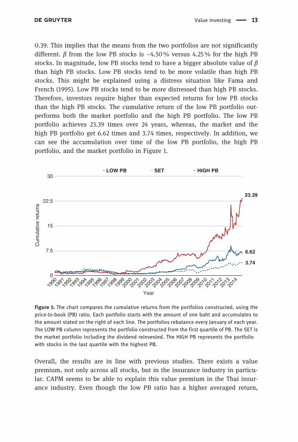
0.39. This implies that the means from the two portfolios are not significantlydifferent. β from the low PB stocks is –4.50% versus 4.25% for the high PBstocks. In magnitude, low PB stocks tend to have a bigger absolute value of βthan high PB stocks. Low PB stocks tend to be more volatile than high PBstocks. This might be explained using a distress situation like Fama andFrench (1995). Low PB stocks tend to be more distressed than high PB stocks.Therefore, investors require higher than expected returns for low PB stocksthan the high PB stocks. The cumulative return of the low PB portfolio out-performs both the market portfolio and the high PB portfolio. The low PBportfolio achieves 23.39 times over 24 years, whereas, the market and thehigh PB portfolio get 6.62 times and 3.74 times, respectively. In addition, wecan see the accumulation over time of the low PB portfolio, the high PBportfolio, and the market portfolio in Figure 1.

Overall, the results are in line with previous studies. There exists a valuepremium, not only across all stocks, but in the insurance industry in particu-lar. CAPM seems to be able to explain this value premium in the Thai insur-ance industry. Even though the low PB ratio has a higher averaged return,

6.62

3.74

Cum

ulat

ive

retu

rns

7.5

15

22.5

0

30

Year19

9019

9119

9219

9319

9419

9519

9619

9719

9819

9920

0020

0120

0220

0320

0420

0520

0620

0720

0820

0920

1020

1120

1220

1320

14

LOW PB SET HIGH PB

23.39

Figure 1: The chart compares the cumulative returns from the portfolios constructed, using theprice-to-book (PB) ratio. Each portfolio starts with the amount of one baht and accumulates tothe amount stated on the right of each line. The portfolios rebalance every January of each year.The LOW PB column represents the portfolio constructed from the first quartile of PB. The SET isthe market portfolio including the dividend reinvested. The HIGH PB represents the portfoliowith stocks in the last quartile with the highest PB.

Value Investing 13

investors face higher volatility by holding these stocks. The portfolio of low PBstocks have a deeper worst month than the high PB stocks. On the other hand,the low PB stocks have the best returns in a single month. However, low PBinsurers’ stocks cumulatively outperform the high PB insurers’ stocks by awide margin.

4.2 Portfolios Constructed from Price-to-Earning Ratio

The following is the result of the portfolios’ returns constructed from the price-to-earnings (PE) ratio. According to Table 3, the portfolio contains stocks withlow PE that outperform the portfolio that consists of high PE, based on themonthly arithmetic average, the annual geometric average, and the monthlyexcess average. The low PE portfolio achieves 3.15% arithmetic average com-pared to 0.96% of the high PE portfolio. Low PE stocks give 41.21% geometricaverage per year compared to 10.03% of the high PE stocks. The difference onthe geometric average is very wide. The low PE portfolio has the worst return foreach month (–21.51%) compared to the high PE stocks (–20.77%). In addition,low PE stocks have a much higher maximum monthly return (68.11%) higher

Table 3: Portfolios constructed from price-to-earning ratio.

LOW PE SET HIGH PE

Min (per month) (%) −. −. −.Max (per month) (%) . . .Arithematic average (per month) (%) . . .Geometric average (per year) (%) . . .Volatility (per month) (%) . . .VaR95% (per month) (%) −. −. −.Average (Ri − Rf ) (per month) (%) . . .Sharpe ratio (per month) (%) . . .β to SET (%) . .Cumulative return of Baht . . .

Note: This table shows information resulting from the construction of portfolios from sorting theprice-to-earnings ratio. The portfolios are rebalanced every January. The first column, LOW PE,represents the first quartile of PE ratios. The second column, SET is the market portfolio includingdividends reinvested. The third column, HIGH PE, represents the last quartile of PE ratios. The tableshows all statistics from each portfolio. Volatility is the standard deviation of themonthly returns ofeach portfolio. VaR95% is the first five percentile of the monthly returns. Sharpe ratio is defined asrp − rfσp

. Beta of the portfolio is calculated from βp =COVðrp, rmÞ

σ2m

. rp is the per-month-return of the

portfolio p. rf is the return of risk-free interest rate per month. σp is the volatility of portfolio p.

14 S. Nettayanun

than the high PE stocks (38.18%). To summarize, on average, low PE stocks tendto have a higher average than high PE stocks. During the bad months, the twoportfolios seem to have similar returns. However, the low PE ratio portfolio has ahigh return during the best month.

Adjusting for volatility, low PE stocks have a volatility of 9.73% comparedto 6.51% for the high PE stocks. An F-test was used to validate the equality ofvariances between the low PE and the high PE portfolios. The p-value of theF-test is 8.58 × 10− 9 with the F-statistics at 0.44. This implies that the volatility oflow PE stocks is different from the high PE stocks. A t-test was also performed,assuming unequal variances from F-test, to check whether the means of the twoportfolios are the same. The test gives t-statistics at 2.68 and p-value of 0.004.This implies that we can reject the null hypothesis that the means from the twoportfolios are the same at 0.01 level. β derived from the low PE stocks is 5.43%versus 1.73% for the high PE stocks. This is in line with the volatility of eachportfolio. Low PE stocks tend to be more volatile than high PE stocks. This is inline with the results constructed using PB ratios. In addition, the low PE stockportfolio has a higher VaR95%, which indicates less than 95% confidence thatthe risk of loss in return for a particular month of the low PE portfolio is lowerthan the high PE portfolio, and the market portfolio. Therefore, these resultscannot be fully explained by reasoning that higher price risk should be compen-sated by higher expected return.

The cumulative return of the low PE portfolio outperforms both the marketportfolio and the high PE portfolio. The low PE ratio achieves 250.06 times over16 years. The market and the high PE portfolio get 6.77 times and 4.62 times,respectively. In addition, figure 2 illustrates the cumulative return and themovement pattern of the low PE portfolio, the high PE portfolio, and the marketportfolio.

Overall, the results are in line with previous studies that show a valuepremium in the Thai insurance industry. Although value premium can beexplained by having higher volatility in stock prices, it cannot be explainedfrom the perspective of the minimum return and the value at risk. However, lowPE stocks in the insurance industry outperform the high PE stocks by a widemargin in terms of cumulative returns over a period of 16 years.13

13 The data of earnings for each stock started in 1997. Therefore, there are only about 16 yearsto accumulate returns. This is different from the PB case. The PB ratios have been availablesince 1990. There are 24 years for portfolio construction in the PB case.

Value Investing 15

4.3 Portfolios Constructed from Three-Year CyclicallyAdjusted Price-to-Earnings Ratio

The following are the results from portfolios constructed from the three-yearcyclically adjusted price-to-earnings ratio. According to Table 4, a portfolioconsisting of stocks with a low level of CAPE3 outperforms a portfolio consistingof high CAPE3, based on the monthly arithmetic average, the annual geometricaverage, and the excess average. The low CAPE3 portfolio achieves a 2.31%arithmetic average compared to 1.42% for the high CAPE3 portfolio. Low CAPE3stocks give a 28.31% geometric average per year versus 16.83% for high CAPE3stocks. The low CAPE3 portfolio has the worst return (–34.14%) for each monthand is lower than the high CAPE3 stocks (–22.96%). In addition, low CAPE3stocks have a much higher best monthly return (59.64%) than the high CAPE3stocks (33.68%).

6.77

250.06

4.62

Cum

ulat

ive

Ret

urns

75

150

225

0

300

Year19

9819

9920

0020

0120

0220

0320

0420

0520

0620

0720

0820

0920

1020

1120

1220

1320

14

LOW PE SET HIGH PE

Figure 2: The chart compares cumulative returns from the portfolios constructed using theprice-to-earnings (PE) ratio. Each portfolio starts with the amount of one baht and accumulatesto the amount stated on the right of each line. The portfolios rebalance every January of eachyear. The LOW PE represents the portfolio constructed from the first quartile stocks with thelowest PE. The SET is the market portfolio including dividend reinvested. The HIGH PE repre-sents the portfolio using stocks in the last quartile with the highest PE.

16 S. Nettayanun

Adjusting for volatility, low CAPE3 stocks have a volatility of 8.90%versus 6.50% forhigh CAPE3 stocks. The author performed the F-test to validate the equality ofvariances between the low CAPE3 and the high CAPE3 portfolios. The p-value ofthe F-test is 1.56 × 10− 5 with the F-statistics at 0.53. This implies that the volatility oflow CAPE3 stocks is different from the high CAPE3 stocks. The author performed thet-test, assuming unequal variances from F-test, to check whether the means of thetwo portfolios are the same. The test gives t-statistics at 1.08 and p-value of 0.28. Thisimplies that the means from the two portfolios are not significantly different. β fromthe low PE stocks is –1.71% and 3.25% for the high CAPE3 stocks. This is in line withthe volatility of each portfolio. Even though the volatility of the low CAPE3 stocks ishigher than the high CAPE3, the β result is the reverse. This implies that the volatilitydoes not quite explain the value premium when we use CAPE3. The low CAPE3portfolio outperforms the high CAPE3 under Sharpe ratio. Therefore, the result thathigher volatility should be compensated by a higher than expected return cannot befully explained by the CAPM.

The cumulative return of the low CAPE3 portfolio outperforms both themarket portfolio and the high CAPE3 portfolio. The low PE portfolio achieves

Table 4: Portfolios constructed from three-year cyclically adjusted price-to-earnings ratio.

LOW CAPE SET HIGH CAPE

Min (per month) −.% −.% −.%Max (per month) .% .% .%Arithematic Average (per month) .% .% .%Geometric Average (per year) .% .% .%Volatility (per month) .% .% .%VaR95% (per month) −.% −.% −.%Average (Ri − Rf ) (per month) .% .% .%Sharpe Ratio (per month) .% .% .%β to SET −.% .%Cumulative Return of Baht . . .

Note: This table shows information resulting from the construction of portfolios by sorting thethree-year cyclically adjusted price-to-earnings ratio. The portfolios are rebalanced everyJanuary. The first column, LOW CAPE3, represents the first quartile of CAPE3 ratios. The secondcolumn, SET, is the market portfolio, including dividends reinvested. The third column, HIGHCAPE3, represents the last quartile of CAPE3 ratios. The table shows all statistics from eachportfolio. Volatility is the standard deviation of the monthly returns of each portfolio. VaR95% is

the first five percentile of the monthly returns. Sharpe ratio is defined as rp − rfσp

. Beta of the

portfolio is calculated from βp =COVðrp, rmÞ

σ2m

. rp is the per-month-return of the portfolio p. rf is the

return from risk-free interest rate per month. σp is the volatility of portfolio p.

Value Investing 17

32.78 times over 14 years, whereas, the market and the high CAPE3 portfoliosachieve 5.07 times and 8.82 times, respectively. In addition, figure 3 illustratesthe cumulative return and the movement pattern of the low CAPE3 portfolio, thehigh CAPE3 portfolio, and the market portfolio.

Overall, there is a value premium as a result of using CAPE3, although it canbe explained by having higher volatility in stock prices. In addition, using theSharpe ratio, the low CAPE3 stocks still outperform the high CAPE3.Interestingly, both the low and high CAPE3 stocks outperform the market asa whole. This is due to the fact that the insurance industry outperformsthe market as a whole during the period used. The setback of this result isdue to the shorter time period as we lose about three years of data foraveraging the lagged earnings. The results would be more reliable if therewere a longer time period.

8.82

32.78

5.07

Cum

ulat

ive

Ret

urns

10

20

30

0

40

Year20

0020

0120

0220

0320

0420

0520

0620

0720

0820

0920

1020

1120

1220

1320

14

LOW CAPE3 SET HIGH CAPE3

Figure 3: The chart compares cumulative returns from the portfolios constructed using CAPE3.Each portfolio starts with the amount of one baht and accumulates to the amount stated on theright of each line. The portfolios rebalance every January of each year. The HIGH CAPE3represents the portfolio constructed from the first quartile stocks with the lowest CAPE3 ratios.The SET is the market portfolio including dividend reinvested. The HIGH CAPE3 represents theportfolio using stocks in the last quartile with the highest CAPE3.

18 S. Nettayanun

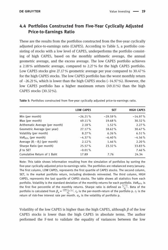
4.4 Portfolios Constructed from Five-Year Cyclically AdjustedPrice-to-Earnings Ratio

These are the results from the portfolios constructed from the five-year cyclicallyadjusted price-to-earnings ratio (CAPE5). According to Table 5, a portfolio con-sisting of stocks with a low level of CAPE5, underperforms the portfolio consist-ing of high CAPE5, based on the monthly arithmetic average, the annualgeometric average, and the excess average. The low CAPE5 portfolio achievesa 2.18% arithmetic average, compared to 2.27% for the high CAPE5 portfolio.Low CAPE5 stocks give 27.17% geometric average per year compared to 30.47%for the high CAPE5 stocks. The low CAPE5 portfolio has the worst monthly returnof –26.21%, which is lower than the high CAPE5 stocks (–14.97%). However, thelow CAPE5 portfolio has a higher maximum return (49.11%) than the highCAPE5 stocks (30.32%).

Volatility of the low CAPE5 is higher than the high CAPE5, although β of the lowCAPE5 stocks is lower than the high CAPE5 in absolute terms. The authorperformed the F-test to validate the equality of variances between the low

Table 5: Portfolios constructed from five-year cyclically adjusted price-to-earnings ratio.

LOW CAPE SET HIGH CAPE

Min (per month) −.% −.% −.%Max (per month) .% .% .%Arithematic Average (per month) .% .% .%Geometric Average (per year) .% .% .%Volatility (per month) .% .% .%VaR95% (per month) −.% −.% −.%Average (Ri − Rf ) (per month) .% .% .%Sharpe Ratio (per month) .% .% .%β to SET −.% .%Cumulative Return of Baht . . .

Note: This table shows information resulting from the simulation of portfolios by sorting thefive-year cyclically adjusted price-to-earnings ratio. The portfolios are rebalanced every January.The first column, LOW CAPE5, represents the first quartile of CAPE5 stocks. The second column,SET, is the market portfolio return, including dividends reinvested. The third column, HIGHCAPE5, represents the last quartile of CAPE5 stocks. The table shows all statistics from eachportfolio. Volatility is the standard deviation of the monthly returns for each portfolio. VaR95% isthe first five percentile of the monthly returns. Sharpe ratio is defined as rp − rf

σp. Beta of the

portfolio is calculated from βp =COVðrp, rmÞ

σ2m

. rp is the per-month-return of the portfolio p. rf is thereturn of risk-free interest rate per month. σp is the volatility of portfolio p.

Value Investing 19

CAPE5 and the high CAPE5 portfolios. The p-value of the F-test is 0.002 with theF-statistics at 0.62. This implies that the volatility of low CAPE5 stocks isdifferent from the high CAPE5 stocks. A t-test was performed, assuming unequalvariances from F-test, to check whether the means of the two portfolios are thesame. The test gives t-statistics at 0.10 and p-value of 0.92. This implies that themeans from the two portfolios are not significantly different. The low CAPE5stocks underperform in both Sharpe ratio and cumulative return. Hence, there isno value premium using the CAPE5 measure. CAPE10, using the 10-year averagesaw a similar result. One explanation of this result might be due to the under-writing standard of insurance companies. Using the long-term average of earn-ings might not reflect the true fundamental value, either going forward orcurrently embedded in the insurer. Therefore, using earnings data that go toofar back in time does not represent the true underlying earning power of the Thaiinsurance firms. Figure 4 shows the cumulative returns from the low CAPE5, thehigh CAPE5, and the market portfolios.

24.34

7.76

17.89

Cum

ulat

ive

Ret

urns

7.5

15

22.5

0

30

Year20

0220

0320

0420

0520

0620

0720

0820

0920

1020

1120

1220

1320

14

LOW CAPE5 SET HIGH CAPE5

Figure 4: The chart compares cumulative returns from the portfolios constructed using theCAPE5 year ratio. Each portfolio starts with the amount of one baht and accumulates to theamount stated on the right of each line. The portfolios rebalance every January of each year. TheLOW CAPE5 represents the portfolio constructed from the first quartile stocks with the lowestCAPE5. The SET is the market portfolio including dividend reinvested. The HIGH CAPE5 repre-sents the portfolio using stocks in the last quartile with the highest CAPE5.

20 S. Nettayanun

4.5 All Measures

Figure 5 shows the cumulative returns of various value portfolios constructedfrom different value measures. The timeframe starts in 2002 because CAPE5 wasavailable since that year. All of the value measures outperform the returns of theThai stock market. According to the figure, the PE ratio outperforms other valuemeasures. Low PB ratio is the worst among various measures but still outper-forms the market. Therefore, using a low PE ratio might give the best indicator ofvalue among insurer stocks.

Cum

ulat

ive

Ret

urns

0

12

24

36

48

60

Year20

0220

0320

0420

0520

0620

0720

0820

0920

1020

1120

1220

1320

14

LOW PB LOW PE LOW CAPE3 LOW CAPE5 Insurance Industry SET

Figure 5: The chart compares cumulative returns from the portfolios constructed using stockswith a low value indicator. Each portfolio starts with the amount of one baht and accumulatesto the amount stated on the right of each line. The portfolios rebalance every January of eachyear. The LOW PB column represents the portfolio constructed from the first quartile of PBratios. The SET is the market portfolio including dividend reinvested. The LOW PE represents theportfolio constructed from the first quartile stocks with the lowest PE. The LOW CAPE3 repre-sents the portfolio constructed from the first quartile stocks with the lowest CAPE3. The LOWCAPE5 represents the portfolio constructed from the first quartile stocks with the lowest CAPE5.The SET is the market portfolio including dividend reinvested. The Insurance Industry includesthe dividend reinvested. The insurance portfolio is constructed using the returns of all insur-ance companies in the Thai stock market.

Value Investing 21

4.6 Stability of the Value Strategy with Financial Crises:A Robust Check

This section studies the stability of the value portfolio before and after thefinancial crises. It captures the performance of the value portfolio, focusing atthe pre and post-crisis events. The Thailand stock market experienced somesignificant drops during the Asian financial crisis of 1997, and the globalfinancial crisis of 2008–2009. According to the SET index data,14 around theAsian financial crisis, it reached the highest point at 1528.83 in October 1994.Then it tumbled to 214 in August of 1998. Then again, around the globalfinancial crisis, it reached the highest point at 907.28 in October 2007. Then ittumbled to 431.5 in March 2009. Therefore, the study splits the timeframe intothree periods. The first period starts in the beginning of 1990 and extends to theend of 1996. The second period starts at the beginning of 1997 and extends to theend of 2008. Finally, the last period starts at the beginning of 2009 andcontinues until the end of 2014. The criteria to split them is that 1997 and2009 are the points in which the market seemed to be in panic. The onlyvalue measure that is available from 1990 to 2014 is the PB ratio. Therefore,the study focuses the result of value stock using the PB ratio and how it worksacross all these crises.

Overall, the value investing strategy is mostly a winning strategy over thesethree periods, according to Table 6. These results are similar when using adataset from 1990–2014, although, the value premium is not quite apparent inperiod 1 (from 1990 to 1996). The arithmetic monthly average of low PB stocks islower than the high PB stocks. The t-test, assuming different variances, gives t-statistics of 0.05 and a p-value of 95.64%. Therefore, it cannot reject the nullhypothesis that the means are equal. However, the low PB portfolio still giveshigher geometric average and higher cumulative return than the high PB port-folio. The magnitude of value premium from 1990 to 1996 is not obvious andmight be due to the fact that there are only 2 to 3 stocks in the portfolios for theyear 1990 and 1991 respectively. This is due to the low number of insurancestocks in the Thai stock exchange. The noises of the returns might be too high togive clear characteristics of the low and the high PB stocks. Hence, it does notshow signs of value premium from 1990 to 1996.

On the other hand, an obvious value premium occurs in the period afterthe Asian financial crisis and before the global financial crisis (1997–2008). The

14 See http://www.set.or.th/en/market/market–statistics.html

22 S. Nettayanun

Table 6: Portfolios constructed from price-to-book ratio separated by the financial crises.

LOW PB SET HIGH PB

Period : –Min (per month) −.% −.% −.%Max (per month) .% .% .%Arithematic Average (per month) .% .% .%Geometric Average (per year) .% .% .%Volatility (per month) .% .% .%Average (Ri − Rf ) (per month) −.% .% .%Sharpe Ratio (per month) −.% .% .%VaR95% (per month) −.% −.% −.%β to SET .% .%Cumulative Return of Baht . . .

Period : –Min (per month) −.% −.% −.%Max (per month) .% .% .%Arithematic Average (per month) .% .% .%Geometric Average (per year) .% −.% .%Volatility (per month) .% .% .%VaR95% (per month) −.% −.% −.%Average (Ri − Rf ) (per month) .% .% .%Sharpe Ratio (per month) .% .% .%β to SET −.% .%Cumulative Return of Baht . . .

Period : –Min (per month) −.% −.% −.%Max (per month) .% .% .%Arithematic Average (per month) .% .% .%Geometric Average (per year) .% .% .%Volatility (per month) .% .% .%VaR95% (per month) −.% −.% −.%Average (Ri − Rf ) (per month) .% .% .%Sharpe Ratio (per month) .% .% .%β to SET −.% −.%Cumulative Return of Baht . . .

Note: This table shows information resulting from the construction of portfolios sorting theprice-to-book ratio. It splits time periods by the occurrences of financial crises. The first period isfrom 1990 to 1996. The second period is from 1997 to 2008. The last period is from 2009 to 2014.The portfolios were rebalanced in the beginning of January every year. The first column, LOW PB,represents the portfolio constructed from the first quartile of PB ratios. The second column, SET, isthe market portfolio with the dividends reinvested. The third column, HIGH PB, represents the lastquartile of PB ratios. The table shows all statistics from each portfolio. Volatility is the standarddeviation of the monthly returns of each portfolio. VaR95% is the first five percentile of the monthly

returns. The Sharpe ratio is defined as. rp − rfσm

. Beta of the portfolio is calculated from βp =COVðrp , rmÞ

σ2p

.

rp is the per-month-return of the portfolio p. rf is the return of risk-free interest rate permonth. σp is

the volatility of portfolio p.

Value Investing 23

value portfolio greatly outperforms the growth portfolio across all performancemeasures. Although, the t-test assuming different variances, has a p-value of0.13, we cannot imply that the returns are different. The geometric average ismuch higher for the value stocks. There is also evidence of value premium from2009 to 2014. The value and growth stocks seem to underperform the SET indexduring this period. However, value stocks still outperform the growth stock from2009 to 2014. Overall, the value investing strategy seems to work well, evencontrolling for financial crises.

5 Can Value Premium Be Explained by CAPM?

According to the capital asset pricing model (CAPM), higher expectations ofreturns compensate for higher risk. CAPM uses the price’s β to measure the riskof each stock. Value stocks result in higher average returns. Therefore, weshould expect to observe higher β for the value portfolio. However, researchershave found the opposite. For example, Fama and French (2006) find that CAPMfails to capture value premium. An examination of whether CAPM can fullycapture value premium is explored in this section.

The following model is used in order to explore the relationship betweenvalue premium and CAPM:

RpðtÞ−Rf ðtÞ= α+ βMarket½RMarketðtÞ−Rf ðtÞ�+ εðtÞ. [2]

The excess returns on the left-hand side of eq. [2] are regressed on the excessreturns of the Stock Exchange of Thailand returns including dividends. The risk-free rates Rf ðtÞ are obtained from the Bank of Thailand’s website. According toTable 7, CAPM does not fully explain the value premium. The CAPM αs are allpositive and significant for the low PB, low PE, and the low CAPE3 that exhibitsvalue premium, as discussed in the previous sections. In addition, there is amixed result, suggesting that value portfolios should have higher βs than thegrowth portfolios. Using PB and CAPE3 measures, βs in the value portfolios aresmaller than the growth portfolios. However, using PE as a measure, the growthportfolio has lower β than the value portfolio. Therefore, if volatility of theportfolio is the measure for risk, we cannot conclude that the value portfolioachieves higher returns than the growth portfolio due to risk. The R2’s are alsolow in all the cases. Therefore, market excess returns do a poor job in explainingthe portfolio’s excess returns.

24 S. Nettayanun

Table 8 is the same as Table 7 except the Asia market returns are used instead ofthe SET index’s returns. Asia market returns and Asia risk-free rates are fromKenneth French’s website. Again, CAPM does not fully explain the value pre-mium. All the α’s of the value portfolios are positive and significant. Valueportfolios have higher βs than the growth portfolios in absolute terms and inall cases. Therefore, using the Asia market index to capture the portfolio returnshas the same results as implied by CAPM. However, R2’s are low for all the casessimilar to the previous case when the SET index returns were used. Therefore,

Table 7: CAPM using SET index.

Portfolio α βSET R2 F-Stat P-Val Obs Year

LOW PB .** −. . . . –[.] [–.]

HIGH PB . . . . . –[.] [.]

LOW PE .*** . . . . –[.] [.]

HIGH PE .* . . . . –[.] [.]

LOW CAPE .*** −. . . . –[.] [–.]

HIGH CAPE .*** . . . . –[.] [.]

Note: This table shows information resulting from OLS regressions of the value portfolio excessreturns, constructed from PB, PE and CAPE3, based on SET market index excess returns,including dividends. LOW PB is the portfolio containing the lowest quartile of PB. HIGH PB isthe portfolio containing stocks with the highest quartile of PB. LOW PE is the portfolio consist-ing of stocks with the lowest quartile of PE. HIGH PE is a portfolio consisting of stocks with thehighest quartile of PE. LOW CAPE3 is a portfolio that contains the lowest quartile of CAPE3stocks. Lastly, HIGH CAPE3 is a portfolio containing high CAPE3 stocks. α column represents theconstant coefficients from all OLS regressions. βSET is the column that contains the coefficientsof the SET index excess returns, including dividends. R2 is the column that represents the R2

value of each regression. F −Stat is the value of the F-statistics to test whether the βSET shouldbe zero. P −Val is the column that represents the p-value from the F-test. Obs is the observa-tion column that represents the number of observations in each particular regression. Year isthe column to represent the year for which data was used, due to the availability of PB, PE andCAPE3. The numbers in square brackets are the t-statistics to test whether each coefficient issignificantly different from zero. *,**, and *** represent the significant levels of 0.10, 0.05, and0.01, respectively, from the t-tests.

Value Investing 25

Asian market index excess returns do a poor job in explaining the portfolios’excess returns.

Next, the global portfolio returns and global risk-free rates from KennethFrench’s website are used to test whether value premium can be explained bythe global market index, as shown in Table 9. According to Table αs are allpositive and significant for the value portfolio. Therefore, CAPM, using globalmarket returns, does not fully explain the value anomaly. In addition, βs in thevalue portfolios is not shown to be more than the growth portfolio in all cases inabsolute terms. In the PE case, β of the portfolio is lower than the growth

Table 8: CAPM using Asia market index.

Portfolio α βAsia R2 F-Stat P-Val Obs Year

LOW PB .** –. . . . –. –.

HIGH PB . . . . . –. .

LOW PE .*** –. . . . –. –.

HIGH PE .* –. . . . –. –.

LOW CAPE .*** –. . . . –. –.

HIGH CAPE .*** . . . . –. .

Note: This table shows information resulting from OLS regressions of value portfolio excessreturns, constructed from PB, PE and CAPE3, based on the Asia market index excessreturns from Kenneth French’s website. LOW PB is the portfolio containing the lowest quartileof PB. HIGH PB is a portfolio containing stocks with the highest quartile of PB. LOW PE is theportfolio consisting of stocks with the lowest quartile of PE. HIGH PE is a portfolio consisting ofstocks with the highest quartile of PE. LOW CAPE3 is a portfolio that contains the lowestquartile of CAPE3 stocks. Lastly, HIGH CAPE3 is a portfolio containing high CAPE3 stocks. Theα column represents the constant coefficients from all OLS regressions. βAsia is a column thatcontains the coefficients of the Asia market excess returns. R2 is the column that represents theR2 value of each regression. F −Stat is the value of the F-statistics to test whether the βAsia

should be zero. P −Val is the column that represents the p-value from the F-test. Obs is theobservation column that represents the number of observations in each particular regression.Year is the column that represents the year for which data was used due to the availability ofPB, PE and CAPE3. The numbers in square brackets are the t-statistics to test whether eachcoefficient is significantly different from zero. *,**, and *** represent the significant levels of0.10, 0.05, and 0.01, respectively, from the t-tests.

26 S. Nettayanun

portfolio. Therefore, if we use price volatility as a proxy for risks, we cannotconclude that the value portfolio is riskier than the growth portfolio.

According to Tables 7, 8 and 9, it appears that CAPM does not fully explainthe value premium. αs are all positive and significant using all of the market’sreturns. In addition, βs in the value portfolios are not always higher than thegrowth portfolios, as CAPM predicts. This result is similar to Fama and French(2006) that states that CAPM fails to capture value anomalies. Therefore, adiscussion to try to explain the value premium, using the Fama-French three-factor model, will follow in the next section.

Table 9: CAPM using global market index.

Portfolio α βGlobal R2 F-Stat P-Val Obs Year

LOW PB .** . . . . –. –.

HIGH PB . . . . . –. –.

LOW PE .*** . . . . –. .

HIGH PE .* –. . . . –. –.

LOW CAPE .*** –. . . . –. –.

HIGH CAPE .** . . . . –. .

Note: This table shows information resulting from OLS regressions of value-portfolio excessreturns constructed from PB, PE and CAPE3, based on global market index excess returns fromKenneth French’s website. LOW PB is the portfolio containing the lowest quartile of PB. HIGH PBis a portfolio containing stocks with the highest quartile of PB. LOW PE is the portfolioconsisting of stocks with the lowest quartile of PE. HIGH PE is a portfolio consisting of stockswith the highest quartile of PE. LOW CAPE3 is a portfolio that contains the lowest quartile ofCAPE3 stocks. Lastly, HIGH CAPE3 is a portfolio containing high CAPE3 stocks. The α columnrepresents the constant coefficients from all OLS regressions. βGlobal is a column that containsthe coefficients of the global market excess returns. R2 is the column that represents the R2

value of each regression. F −Stat is the value of the F-statistics to test whether the βGlobal

should be zero. P −Val is the column that represents the p-value from the F-test. Obs is theobservation column that represents the number of observations in each particular regression.Year is the column to represent the year for which data was used due to the availability of PB,PE and CAPE3. The numbers in square brackets are the t-statistics to test whether eachcoefficient is significantly different from zero. *,**, and *** represent the significant levels of0.10, 0.05, and 0.01, respectively, from the t-tests.

Value Investing 27

6 Can Fama-French Three-Factor Model Explainthe Value Anomaly?

Next, the Fama-French three-factor model is used to explain the value premiumintroduced in Fama and French (1993). In particular, the following equation isregressed:

RpðtÞ−Rf ðtÞ= α+ βMarket½RMarketðtÞ−Rf ðtÞ�+ βSML*RSMLðtÞ + βHML*RHMLðtÞ+ εðtÞ.[3]

In addition to market excess returns in the CAPM model, the factors are smallminus large (SML) and high minus low (HML). These factors use data fromKenneth French’s website. SML is the portfolio returns from investing in smallstocks and shorting large stocks. HML is the portfolio returns from investing inhigh book-to-market stocks and shorting low book-to-market stocks. If the Fama-French three-factor model can explain the value anomaly, the author of thisstudy would expect the α to be indifferent from zero. In addition, as theinsurance portfolio construction is based on value, it could be expected thatthe HML factor helps to explain the value anomaly. The Asia and global Fama-French three-factor returns are extracted from Kenneth French’s website. TheAsia factors exclude Japan, due to the fact that Japan has not exhibited valuepremium in the market over the past 26 years.

According to Table 10, the Fama-French three-factor model, using the Asiadata excluding Japan, still does not capture the value anomaly. The intercept orα is still significantly positive. The R2 is higher than previous sections fromCAPM, although this is what is expected as more variables are added to theregression. Observations are different in each measure (PB, PE, and CAPE3) dueto the availability of each measure. The only factor that is significant is from theuse of CAPE3. The βHML is positive and significant, which is counterintuitive.βHML should be positive for the low CAPE3 case, as expected.

According to Table 11, using the global Fama-French three-factor model stillfails to explain the anomaly of insurance value portfolios. The α’s or the inter-cept of the regression are all positive and significant for the value portfolio. Inaddition, the growth portfolio has positive and significant α as well. However,the size factor has a positive and significant coefficient for the low PB case. Thisimplies that size factor can partially explain the value premium, although onlyin the PB case.

Overall, the global and Asia Fama-French three-factor models do not fullyexplain the value premiums of insurance value portfolios. The explanation ofthis finding could involve several issues, including the number of stocks in the

28 S. Nettayanun

value portfolio and the factors themselves. On average, each value portfolioconsists of about four stocks. These stocks can be volatile in comparison to thestudies of Fama and French (1993) that contain hundreds of stocks. The noise inthe regression is so high that the Fama-French three-factor models fail to findthe relationship between portfolio returns and the factors. The implication ofthis is that if investors concentrate on a few stocks instead of many, they canoutperform the market with low portfolio volatility. In addition, as the availableFama-French three-factor models were used, globally and for Asia, they mightnot be able to provide the explanation within the local market of Thailand.

Table 10: Asia market Fama-French three-factor model.

Portfolio α βAsia βSMB βHML R2 F-Stat P-Val Obs Year

LOW PB .* –. . . . . . –. –. . .

HIGH PB . . . . . . . –. . . .

LOW PE .*** –. . . . . . –. –. . .

HIGH PE . –. . . . . . –. –. . .

LOW CAPE .*** –. . . . . . –. –. . .

HIGH CAPE .* . –. .** . . . –. . –. .

Note: This table shows information resulting from OLS regressions of value-portfolio excessreturns constructed from PB, PE and CAPE3 on the Fama-French three-factor model. Particularly,it uses three factors including Asia market excess returns, SML, and HML factors from KennethFrench’s website. LOW PB is the portfolio containing the lowest quartile of PB. HIGH PB is aportfolio containing stocks with the highest quartile of PB. LOW PE is the portfolio consisting ofstocks with the lowest quartile of PE. HIGH PE is a portfolio consisting of stocks with the highestquartile of PE. LOW CAPE3 is a portfolio that contains the lowest quartile of CAPE3 stocks. Lastly,HIGH CAPE3 is a portfolio containing high CAPE3 stocks. α column represents the constantcoefficients from all OLS regressions. βAsia is a column that contains the coefficients of the Asiamarket excess returns. βSMB is a column that contains the size factor of the Fama-French three-factor model. βHML is a column that contains the value factor of the Fama-French three-factormodel. R2 is the column that represents the R2 value of each regression. F −Stat is the value ofthe F-statistics to test whether the βs should be zero. P −Val is the column that represents thep-value from the F-test. Obs is the observation column that represents the number of observa-tions in each particular regression. Year is the column to represent the year for which data wasused due to the availability of PB, PE and CAPE3. The numbers in square brackets are the t-statistics to test whether each coefficient is significantly different from zero. *, **, and ***represent the significant levels of 0.10, 0.05, and 0.01, respectively, from the t-tests.

Value Investing 29

Therefore, it leaves some room for future research to construct a local Fama-French three-factor model to explain this anomaly.

7 Conclusion

The study explores value stocks, specifically for the insurance industry inThailand. According to the results, we can argue that by focusing on a particular

Table 11: Global Fama-French three-factor model.

Portfolio α βGlobal βSMB βHML R2 F-Stat P-Val Obs Year

LOW PB .** –. .** . . . . –. –. . .

HIGH PB . –. .* . . . . –. –. . .

LOW PE .*** . . . . . . –. . . .

HIGH PE . –. .* . . . . –. –. . .

LOW CAPE .*** –. . . . . . –. –. . .

HIGH CAPE .** . . . . . . –. . . .

Note: This table shows information resulting from OLS regressions of value-portfolio excessreturns constructed from PB, PE and CAPE3 on the Fama-French three-factor model. Particularly,it uses three factors, including global market excess returns, SML, and HML factors fromKenneth French’s website. LOW PB is the portfolio containing the lowest quartile of PB. HIGHPB is a portfolio containing stocks with the highest quartile of PB. LOW PE is a portfolioconsisting of stocks with the lowest quartile of PE. HIGH PE is a portfolio consisting of stockswith the highest quartile of PE. LOW CAPE3 is a portfolio that contains the lowest quartile ofCAPE3 stocks. Lastly, HIGH CAPE3 is a portfolio containing high CAPE3 stocks. α columnrepresents the constant coefficients from all OLS regressions. βGlobal is a column that containsthe coefficients of the global market excess returns. βSMB is a column that contains the sizefactor of the Fama-French three-factor model. βHML is a column that contains the value factor ofthe Fama-French three-factor model. R2 is the column that represents the R2 value of eachregression. F −Stat is the value of the F-statistics to test whether the βs should be zero. P −Valis the column that represents the p-value from the F-test. Obs is the observation column thatrepresents the number of observations in each particular regression. Year is a column torepresent the year that data is used due to the availability of PB, PE and CAPE3. The numbersin square brackets are the t-statistics to test whether each coefficient is significantly differentfrom zero. *, **, and *** represent the significant levels of 0.10, 0.05, and 0.01, respectively,from the t-tests.

30 S. Nettayanun

industry, investors can still outperform the market using a value investingstrategy. Similar to previous value studies, this study finds value premiumswithin the Thai insurance industry. Investing in low value measures, such asPE, PB, CAPE3, and CAPE5, outperforms the market, although value premiumdoes not always occur when looking too far back over many years, for examplein the CAPE5 case. Using the traditional PE ratio can be very profitable to beatthe market. This result is similar to Basu (1977). Using the value measure by PBratio does not perform quite as well for insurance stocks, compared to the PEmeasure. However, the study does not consider size, so we cannot draw aconclusion that is similar to Fama and French (1992) that combines size andvalue factors, and absorbs the price-to-earnings factor to predict the returnsfrom the stocks.

According to the results, price volatility from CAPM does not fully explainthe value premium. Value stocks widely outperform the high PE, PB and CAPE3,even when adjusted for volatility and β. Jensen’s α is also higher for the valueportfolio. In addition, the Fama-French three-factor model using global and Asiafactors does not capture the value anomaly. The author of this study suspectsthat this is due to the small number of stocks in the portfolio, and also becausethe factors are not local enough for the Thai market. On the other hand, it showsthat investors can achieve superior results by investing in low PB, PE and CAPE3insurance stocks. It also achieves superior absolute returns with lower portfoliovolatility.

Still, this study has some limitations. First, it focuses particularly on theinsurance industry. It assumes that investors have a circle of competence that isbased on the insurance industry. The study could, therefore be expanded toother industries within the stock market. Second, the number of stocks in theportfolio is arguably small (four, on average). Therefore, this result might bebiased toward this limited dataset. One might argue that this is a result from adata snooping problem. However, one might also argue that in order to beat themarket, there does not need to be a huge amount of stocks in the portfolio,which is the main point of this study. In addition, the study also uses a longperiod of time to construct and rebalance the portfolio. The results that show thevalue portfolio outperforming the growth portfolio seems to be in line withprevious studies of the Thai stock market, such as Sareewiwatthana (2011,2012, 2013).

In addition, there might be other factors in the behavior of investors toexplain the value anomaly. The author leaves it to future research to explorethese issues. In addition, the paper does not incorporate any quality measuresinto constructing the portfolios, as in Novy-Marx (2013) or Novy-Marx (2015),although the pure value portfolio can still outperform the market.

Value Investing 31

Furthermore, circles of competence in other industries should be explored.The obvious choice is the banking industry. There are many aspects in theinsurance industry that are similar to the banking industry. Various valuemeasures can still be used for constructing value portfolios as the bankingindustry also exhibits a cyclical nature. The author suspects that some valuemeasures might not be applicable for non-financial industries. For example,using the CAPE measure might not be appropriate for a growth industry. Theintention of using CAPE for this study is because the insurance industry iscyclical. Therefore, researchers who carry out the circle of competence researchmight have to be cautious when choosing appropriate value measures. After all,the practice of investing in the things that an investor understands, or within acircle of competence, has begun.

Funding: Naresuan University, (Grant / Award Number: ‘R2558C244’)

References

Asness, C., A. Frazzini, R. Israel, and T. Moskowitz 2015. “Fact, Fiction, and Value Investing.”Available at SSRN 2595747.

Asness, C. S., J. Moskowitz, and L. H. Pedersen. 2013. “Value and Momentum Everywhere.”Journal of Finance 68 (3):929–85.

Basu, S. 1977. “Investment Performance of Common Stocks in Relation to Their Price-EarningsRatios: A Test of the Efficient Market Hypothesis.” Journal of Finance 32 (3):663–82.

Bondt, W. F., and R. Thaler. 1985. “Does the Stock Market Overreact?” Journal of Finance40 (3):793–805.

Campbell, J. Y., and R. J. Shiller. 1988. “Stock Prices, Earnings, and Expected Dividends.”The Journal of Finance 43 (3):661–76.

Carnegie, A. 2012. The Autobiography of Andrew Carnegie. Chaleston, SC: CreateSpaceIndependent Publishing Platform.

Cummins, J. D., M. A. Weiss, and H. Zi. 1999. “Organizational Form and Efficiency: TheCoexistence of Stock and Mutual Property-Liability Insurers.” Management Science45 (9):1254–69.

Daniel, K., D. Hirshleifer, and A. Subrahmanyam. 1998. “Investor Psychology and SecurityMarket Under and Overreactions.” Journal of Finance 53 (6):1839–85.

Dodd, D., and B. Graham. 1951. Security Analysis: The Classic 1951 Edition. New York: McGrawHill.

Fama, E. F., and K. R. French. 1992. “The Crosssection of Expected Stock Returns.” Journal ofFinance 47 (2):427–65.

Fama, E. F., and K. R. French. 1993. “Common Risk Factors in the Returns on Stocks andBonds.” Journal of Financial Economics 33:3–56.

Fama, E. F., and K. R. French. 1995. “Size and Book-to-Market Factors in Earnings and Returns.”Journal of Finance 50 (1):131–55.

32 S. Nettayanun

Fama, E. F., and K. R. French. 1996. “Multifactor Explanations of Asset Pricing Anomalies.”Journal of Finance 51 (1):55–84.

Fama, E. F., and K. R. French. 1998. “Value Versus Growth: The International Evidence.” Journalof Finance 53 (6):1975–99.

Fama, E. F., and K. R. French. 2006. “The Value Premium and the CAPM.” Journal of Finance61 (5):2163–85.

Fama, E. F., and K. R. French. 2012. “Size, Value, and Momentum in International StockReturns.” Journal of Financial Economics 105 (3):457–72.

Fama, E. F., and K. R. French. 2015. “A Five-Factor Asset Pricing Model.” Journal of FinancialEconomics 116 (1):1–22.

Frazzini, A., D. Kabiller, and L. H. Pedersen 2013. “Buffett’s Alpha.” Working Paper.Graham, B.. 2003. The Intelligent Investor: The Definitive Book on Value Investing. a Book of

Practical Counsel, Revised 7th ed. New York: Harper & Collins.Lakonishok, J., A. Shleifer, and R. W. Vishny. 1994. “Contrarian Investment, Extrapolation, and

Risk.” Journal of Finance 49 (5):1541–78.Nettayanun, S. 2014. Essays on Strategic Risk Management. Atlanta, GA: Georgia State

University.Novy-Marx, R. 2013. “The Other Side of Value: The Gross Profitability Premium.” Journal of

Financial Economics 108 (1):1–28.Novy-Marx, R. 2015. “Quality Investing.” Working Paper.Piotroski, J. D. 2000. “Value Investing: The Use of Historical Financial Statement Information to

Separate Winners From Losers.” Journal of Accounting Research 38:1–41.Piotroski, J. D., and E. C. So. 2012. “Identifying Expectation Errors in Value/Glamour Strategies:

A Fundamental Analysis Approach.” Review of Financial Studies 25 (9):2841–75.Sareewiwatthana, P. 2011. “Value Investing in Thailand: The Test of Basic Screening Rules.”

International Review of Business Research Papers 7 (4):1–13.Sareewiwatthana, P. 2012. “Value Investing in Thailand: Evidence From the Use of PEG.”

Technology and Investment 3 (2):113–20.Sareewiwatthana, P. 2013. “Common Financial Ratios and Value Investing in Thailand.” Journal

of Finance and Investment Analysis 2 (3):69–85.Sharpe, W. F. 1964. “Capital Asset Prices: A Theory of Market Equilibrium Under Conditions of

Risk.” Journal of Finance 19 (3):425–42.Shleifer, A., and R. W. Vishny. 1997. “The Limits of Arbitrage.” Journal of Finance 52 (1):35–55.

Value Investing 33