Valuation of Near-Market Endogenous Assets∗

Dennis Fixler

The Bureau of Economic Analysis

Ryan Greenaway-McGrevy

The Bureau of Economic Analysis

February 17, 2012

Abstract

For many kinds of assets, the growth rate of the real asset stock is a

nonlinear function of the economic owner’s decision whether to invest or

extract the asset. Examples within the economy are primarily biological

assets, both privately owned (such as those found in aquaculature and

agriculture) and publicly owned or regulated (such as fish stocks, and in

some case, timber stocks.) Optimal exploitation of the asset necessitates

that the future possible growth rates in the asset must be considered when

determining the optimal amount of extraction today. In this sense, the

level of the asset is determined by the economic owner or regulator and

is thus said to be endogenous. This paper considers existing methods for

the valuation of these endogenous assets when observed transaction prices

are lacking. In particular, we consider valuation in a near-market context,

whereby the the economist can only observe income flows from the asset.

This near-market approach to asset valuation is particularly important

for environmental accounting when transaction prices for the asset or the

right to exploit the asset are lacking. We give sufficient restrictions on the

revenue and cost structure of the firm in order to permit asset valuation

based on average profits. In an emprical application, we combine economic

and biomass data to value the US Bering Sea crab fisheries.∗The views expressed herein are those of the authors and not those of the Bureau of

Economic Analysis or the Department of Commerce.

1

1 Introduction.

Obtaining an accurate valuation of a natural resource is central to the United

Nations System of Environmental Economic Accounts (SEEA). A revised SEEA

central framework is due for publication in 2012. The valuation of endogenous

natural assets is an important class of natural resource assets. By endogenous

assets we mean assets whose stocks in part vary by an internal growth process.

One such natural asset that has received a lot of attention in the economics

literature is fisheries. The treatment of fisheries is cast in a capital theoretic

context in which the optimal stock is determined by discounting the benefits

and costs over time subject to the constraints of the growth process. See for

example Scott (1954), Gordon, (1954), Crutchfield and Zellner (1962), and Tur-

vey (1964); the role of these treatments is described in Munro (1992). The

dynamic optimization problem is an offshoot of the Hotelling (1931) and the

models described in Clark (1985).

Other types of natural assets to which this framework could apply is forests,

wild animal preserves, and to some extent this is the problem underlying culti-

vated assets such as herds, vineyards and so on.

The effort in the literature is directed toward determining optimal stock

and optimal extraction. In this paper the focus is on the determination of the

asset value given the optimal stock and extraction. From this asset value we

can then obtain a real measure of the stock of capital. The standard approach

to measuring the stock of capital is to take the initial value, add investments

and subtract depreciation, obsolescence and so on. For the endogenous assets

considered herein may of these additions and subtractions are inherent - the

growth process for fish considers the birth and death of the stock as well as the

extraction that is part of the production process.

Hotelling valuation (HV) is conventionally applied to assets for which the

growth in the quantity of the asset is independent of the decision to extract or

invest in the asset.1 For example, Miller and Upton (1985) apply HV to oil and

gas reserves, while the Integrated Economic-Environmental Satellite Accounts

1We refer the reader to the Appendix for a brief overview of Hotelling valuation applied to

these conventional assets when marginal profits are constant.

2

(IEESAs, 1994a,1994b) produced by the BEA apply HV to both subsoil hydro-

carbon and mineral assets in the US economy. Here the physical quantity of

asset is independent of how much the firm chooses to extract; indeed, the phys-

ical quantity of the asset below the ground is fixed. Yet independence is clearly

not appropriate for other assets in the economy. For example, the growth in

many cultivated biological assets, such as fish raised in fish farms, is dependent

on whether or not the firm chooses to extract some of the asset. We describe

these assets as endogenous in the sense that the firm simultaneously chooses a

sequences of extraction levels and a long-run asset level in order to maximize

the value of the asset. In this paper we consider Hotelling valuation (HV) for

assets with this type of endogenous growth.

Examples of endogenous assets within the economy are primarily biological

assets, both privately owned (such as those found in aquaculture and agricul-

ture) and publicly owned or regulated (such as fish stocks, and in some cases,

timber stocks.) Typically, growth is specified as a function of the level of the

asset stock, so that the economic owner or regulator will simultaneously choose

an extraction level and a asset quantity to maximize the present value of future

profits.2 Value added generated by these assets that fall within this category

contributed just over 1.02% of the US economy over the 1999-2008 period, as

the table below demonstrates. For comparison, oil, gas and mining extraction

together made up 1.13% of the economy. The value added generated by the

entire Agriculture Forestry and Fishing industry was $136,413 million for 2009

(current dollars). If we were to apply a back-of-the-envelope present value calcu-

lation, assuming that all future revenue from the sector would remain the same

(in 2009 dollars), this would place the present value between 3.4 and 1.9 trillion

dollars, using a discount rate of 4% and 7%, respectively. For comparison, the

total market value of all corporations traded on the NYSE was 12 trillion in

August 2010.

2 In some cases growth is specified as a function of the age of the stock. For example Clarke

and Reed (1989) specify the natural growth in trees as a function of the age of the tree.

3

Value Added of selected Industries as % of GDP

Agriculture, Forestry, Oil Mining,

forestry, fishing, and except

fishing, Farms and related Mining gas oil and

Year and hunting activities extraction gas

1998 1.14 0.90 0.24 0.92 0.45 0.32

1999 0.99 0.76 0.23 0.88 0.46 0.31

2000 0.96 0.74 0.22 1.09 0.68 0.28

2001 0.96 0.74 0.22 1.16 0.71 0.27

2002 0.89 0.68 0.21 1.03 0.63 0.26

2003 1.04 0.83 0.21 1.21 0.80 0.25

2004 1.20 1.00 0.21 1.34 0.90 0.26

2005 1.01 0.81 0.20 1.52 1.02 0.29

2006 0.91 0.69 0.22 1.71 1.10 0.30

2007 1.04 0.83 0.22 1.72 1.07 0.31

2008 1.13 0.91 0.22 2.13 1.41 0.34

mean 1.02 0.81 0.22 1.34 0.84 0.29

HV for endogenous assets combines economic theory, describing optimal firm

behavior given a set of constraints, with biological models of the natural world.

In particular, we will require mathematical functions that describe how the asset

grows in response to the extractive decisions of the firm. The models for solving

the firm’s problem are well-established in the literature (see Clark, 2010, for

a detailed overview of so-called “bioeconomic” methods), and this paper will

draw on many of the theories already well established in the literature. In this

sense we are not re-inventing the wheel. Rather, the purpose of the paper is

outline these methods, and discuss what assumptions on the models would be

necessary for us to derive accurate valuation of these assets given an observed

income stream from the asset. The issue is thus seeing how far firm- or industry-

level accounting information can be used to obtain values for endogenous assets.

Such assets will be called “near-market” assets; although transactions prices for

4

the asset itself are lacking, we can observe the price and quantity of the goods

flowing from the asset. We will begin by stating the firm’s extraction problem

within a general and rich model that permits various cost and market structures

on the economic side, and we will initially remain agnostic about the biological

growth function. Having solved the model, we will then outline the weakest

possible assumptions that facilitate asset valuation given the observed income

stream from the asset.

Typically data for the marginal profit of extraction across a range of different

extraction rates is lacking. This would inform us about the profitability of the

firm as we change the amount extracted, and in a dynamic setting, knowledge

of the marginal profitability of extraction is crucial as the firm will select a

sequence of current and future extraction rates in order to maximize the value

of the asset. Instead, one can only usually observe average profit per unit from

extraction of the asset through conventional cost and revenue per unit reports.

In order to infer valuation based on this data, one must impose simplifying

assumptions between the observed average return and the unobserved marginal

return in order to derive a valuation from the data. (See for example, Miller

and Upton, 1985, and Nordhaus and Kokkelenberg, 1999). In what follows we

will outline sufficient assumptions for valuation from average per-unit profit.

Another important factor in solving the optimal control problem of the firm

is the ownership structure of the asset. The firm may take into account how its

extraction this season will affect the future stock level, which in turn will affect

the firm’s profits in beyond the current period. When the number of owners

is sufficiently small, a profit-maximizing firm will take the affect of its current

extraction on the future stock level into account. Consider an aquaculture firm,

for example. The firm has exclusive rights to extract fish from its private tanks.

In contrast, when ownership is sufficiently sparse, so that the effect of the firm’s

extraction on the asset level is very small, a profit-maximizing firm will not take

the affect of its current extraction into account. For example if a wild resource

is permitted to be extracted by some firms through regulation, then the effect

of the firm’s extraction on the stock level is arbitrarily small. If the firm’s take

is sufficiently small the firm may not take into account its current extraction

on the future stock of the asset. Predictably this leads to the firm adopting a

5

higher level of extraction in the short run. Yet increasingly extraction of these

assets is regulated by a central authority. For these assets, the total extraction

(across all firms permitted access) is set by the authority is order to attain

a long-run asset stock level. Of course, the target long-run level may not be

the profit-maximizing level of the asset. Thus we will argue that the first best

option in this eventuality is to operationalize the regulator’s stated goal - if she

has one - into an objective function. A second best option will be to assume

that the authority acts as the optimizer buy choosing the optimal stock level to

maximize firm profits. In either case, we may use firm-level accounting data to

value the resource.

The rest of the paper is organized as follows. In section 2 we outline the

optimal control theory to be used to value the near-market assets. In this section

we will also outline sufficient conditions on firm cost and revenue for valuation

to be possible based on average profitability data. In section 3 we will consider

the specific example of the Bering Sea crab fisheries. Section four concludes.

2 Theory.

We begin by stating the dynamic optimization problem of the representative

firm. Much of what we summarize here has been gleaned from Clarke (2010).

Before we begin it is instructive to define the following notation.

Notation. We define the following.

Ht : extraction (or “harvest”) at time t.

Xt : asset stock at time t.

Vt : value of asset stock at time t.

δ : discount rate.

g (Xt) : growth function for asset stock.

p (Ht) : inverse demand function for Ht.

c (Ht,Xt) : firm cost function.

Firm cost c (Ht,Xt) is a function of both the harvest Ht and the asset

stock Xt at time t. As a function of Ht we are permitting standard increasing

6

marginal costs. Costs are also permitted to be a function of the asset size Xt,

reflecting “search costs”: As abundance of many biological stocks increases, the

costs associated with searching for the asset decrease. This aspect may be more

relevant for “wild” stocks such as fish as opposed to cultivated biological assets.

For search costs we would expect ∂c (Ht,Xt) /∂Xt < 0. Similar flexibility is

permitted in models of optimal extraction of non-renewable assets. For example,

when an oil well is new, oil extraction is cheap as the oil is under pressure and can

be extracted easily (see, for example, chapter 3 of Nordhaus and Kokkelenberg,

1999; Miller and Upton, 1985). In this case ∂c (Ht,Xt) /∂Xt < 0.

We permit the price received by the firm p (Ht) to be a function of the

quantity harvested, thereby permitting the firm to exhibit market power. Firm

profits are given by

π (Ht,Xt) = (p (Ht)− c (Ht,Xt))Ht

Note that profit is not necessarily linear in extraction Ht. Valuation of the asset

boils down to

V0 =

Z ∞0

e−δtπ (Ht,Xt) dt =

Z ∞0

e−δt [(p (Ht)− c (Ht,Xt))Ht] dt. (1)

We must solve for {Ht}∞t=1 and {Xt}∞t=1. The optimal control problem becomesa variation in Hotelling (1931).

2.1 Generalized Hotelling Model.

The firm’s problem is to maximize the objective function;

V0 = max{Ht}∞t=1

Z ∞0

e−δtπ (Ht,Xt) dt, (2)

subject to the constraints

Xt = g (Xt)−Ht,

Xt ≥ 0,

0 ≤ Ht ≤ Hmax.

The current value Hamiltonian is

L (Ht,Xt, ψ) = π (Ht,Xt) + ψt (g (Xt)−Ht) (3)

7

where ψt := eδtλt, and λt is the shadow price for the present value Hamiltonian.

Then the first order conditions (FOCS) are

∂L (Ht,Xt, ψ)

∂Ht= 0

∂L (Ht,Xt, ψ)

∂Xt= δψt − ψt

which under (3) imply that

∂π (Ht,Xt)

∂Ht= ψt, (4)

ψt = δψt −∂π (Ht,Xt)

∂Xt− ψtg

0 (Xt) , (5)

respectively. Eq.(4) says that the marginal value of harvesting must equal the

marginal product of the asset in equilibrium. Eq.(5) can be re-written as

δ =ψtψt+

∂π (Ht,Xt)

∂Xtψt+ g0 (Xt)

which says that the marginal return to delaying extraction (capital gains on

the asset ψtψtplus the effect on profit ∂π(Ht,Xt)

∂Xtψtplus marginal changes in volume

g0 (Xt)) must be equal to the rate of time preference. Combining the results we

have

ψt = (δ − g0 (Xt))∂π (Ht,Xt)

∂Ht− ∂π (Ht,Xt)

∂Xt

Note that if ∂π(Ht,Xt)∂Xt

= 0, the above implies that the shadow price changes at

rate δ − g0 (Xt).

Equilibrium. Equilibrium is defined by setting ψt = 0 and Xt = 0, which

give us our solutions X∗t and H∗t :

g0 (X∗t ) +∂π (H∗t ,X

∗t ) /∂X

∗t

∂π (H∗t ,X∗t ) /∂H

∗t

= δ (6)

g (X∗t ) = H∗t (7)

Together these two equations characterize the amount extracted H∗t as well as

the asset stock X∗t in equilibrium. (H∗t is often referred to as the “economic

sustainable yield”.) Exact expressions require specifying more a precise profit

function π (Ht,Xt) and growth function g (Xt). We address each issue in the

following two sub-sections. After this, we will discuss transition to the equilib-

rium. We will argue that the transition to equilibrium depends on the market

structure.

8

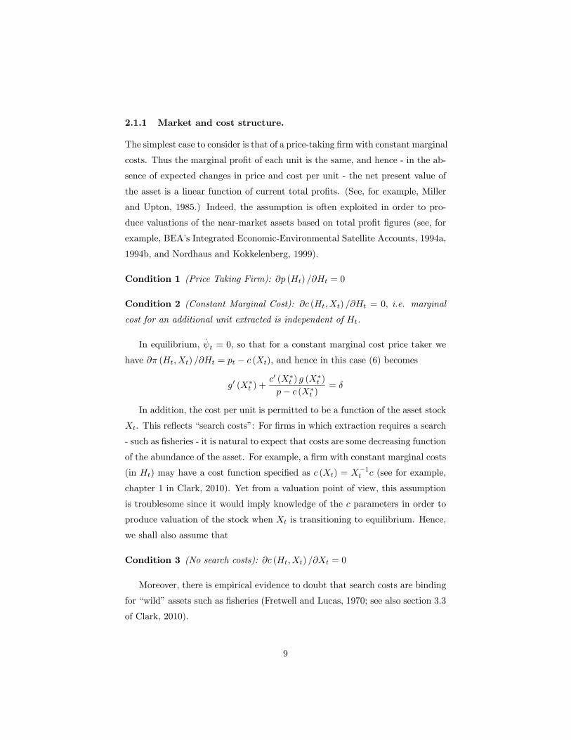
2.1.1 Market and cost structure.

The simplest case to consider is that of a price-taking firm with constant marginal

costs. Thus the marginal profit of each unit is the same, and hence - in the ab-

sence of expected changes in price and cost per unit - the net present value of

the asset is a linear function of current total profits. (See, for example, Miller

and Upton, 1985.) Indeed, the assumption is often exploited in order to pro-

duce valuations of the near-market assets based on total profit figures (see, for

example, BEA’s Integrated Economic-Environmental Satellite Accounts, 1994a,

1994b, and Nordhaus and Kokkelenberg, 1999).

Condition 1 (Price Taking Firm): ∂p (Ht) /∂Ht = 0

Condition 2 (Constant Marginal Cost): ∂c (Ht,Xt) /∂Ht = 0, i.e. marginal

cost for an additional unit extracted is independent of Ht.

In equilibrium, ψt = 0, so that for a constant marginal cost price taker we

have ∂π (Ht,Xt) /∂Ht = pt − c (Xt), and hence in this case (6) becomes

g0 (X∗t ) +c0 (X∗t ) g (X

∗t )

p− c (X∗t )= δ

In addition, the cost per unit is permitted to be a function of the asset stock

Xt. This reflects “search costs”: For firms in which extraction requires a search

- such as fisheries - it is natural to expect that costs are some decreasing function

of the abundance of the asset. For example, a firm with constant marginal costs

(in Ht) may have a cost function specified as c (Xt) = X−1t c (see for example,

chapter 1 in Clark, 2010). Yet from a valuation point of view, this assumption

is troublesome since it would imply knowledge of the c parameters in order to

produce valuation of the stock when Xt is transitioning to equilibrium. Hence,

we shall also assume that

Condition 3 (No search costs): ∂c (Ht,Xt) /∂Xt = 0

Moreover, there is empirical evidence to doubt that search costs are binding

for “wild” assets such as fisheries (Fretwell and Lucas, 1970; see also section 3.3

of Clark, 2010).

9

Thus under this additional assumption (6) becomes

g0 (X∗t ) = δ, (8)

which together with g (X∗t ) = H∗t , characterizes the stock level and extraction

for a given growth function g (Xt). Thus if the asset is at equilibrium X∗t ,

valuation of the asset simplifies to

V0 =

Z ∞0

e−δtπ (H∗t ) dt = (p0 − c0) g (X∗t )

Z ∞0

e−δtdt, (9)

where the second equality holds if we assume that future price and cost per unit

extracted is the same as current price and cost per unit extracted.

2.1.2 Variation in Productive Efficiency.

Much of the empirical literature has examined the cause of variation in efficiency

both across time and firms. For example, Kompas and Che (2005) showed how

the introduction of a transferable quota system resulted in aggregate cost reduc-

tions in the Australian South East Trawl fishery. Kirkley, Squires and Strand

(1998) and Alvarex and Schmidt (2006) examine and test various hypotheses

for the variation in technical efficiency between boats.

Changes in technical efficiency can be incoporated into the model through

the per-unit costs function c (Ht,Xt). Notably the per-unit cost function c (Xt,Ht)

in the general model outlined above is time-invariant. However care must be

taken to distinguish between movements along the cost function from shifts in

the cost function depending on the soruce of increases in efficiency. For ex-

ample, reductions in marginal cost due to a policy-maker restricting catch or

to increased stock levels would represent a movement along the cost function.

Changes in technology and improvements in managerial skill would represent

a shift in the cost function. This could be accounted for by interacting an ad-

ditional variable with the cost function, such as α (t) · c (Ht,Xt). When using

solving the optimal control problem to value a stock, any foreseable secular

trends in the cost function would have to be incorporated into the firm’s prob-

lem, complicating the optimal control problem by adding an additional state

variable α (t).

10

2.1.3 Uncertainty.

The model outlined above is deterministic. In practice the firm faces a variety

of risks; prices can vary, costs can vary, the growth function may be unknown,

and there may be unforeseeable factors that affect the stock (e.g., “catastrophic

losses” in fisheries). The uncertainty associated with these variables would likely

affect the price a buyer would be willing to pay for the asset.

The textbook approach to incorporating uncertainty into the NPV formula

is to adjust the discount rate upwards to reflect risk. The income streams going

forward used in the NPV formula are then the expectation of the income streams

(given that in the stochastic world we no longer know the income streams with

certainty). Clarke and Reed (1989) show formally that bioeconomic asset val-

uation in a Gaussian framework is equivalent to valuation using an adjusted

discount rate and the expected income streams. This naturally raises the is-

sue of what discount rate to use in practice. Further complicating the issue is

the emerging consensus that the discount rate itself varies over time as investor

appetite for risk varies over the business cycle (Cochrane, 2010). This would

suggest that the discount rate needs updating over the business cycle.

The selection of the appropriate discount rate for the costs associated with

climate change at the macro level has been the subject of intense debate. Nord-

haus (1997) characterizes two contrasting approaches, the ‘descriptive approach’

“asks what combination of parameters can rationalize existing rates of returns”

on the assets we observe in the market place. The ‘prescriptive approach’ “be-

gins with a view about time preference and inequality aversion and from this

concludes what the appropriate discount rate is.” The latter approach may be

characterized as normative, the former as positive approaches to select the dis-

count rate. The prescriptive discount rate is often selected to be low on the basis

of ethical arguments, as in the Stern Review (Stern, 2006). As pointed out by

Nordhaus (1997), the two views can be reconciled by considering the scarcity

of the asset in question in the future. That said, Nordhaus (2007) criticizes the

Stern review discount rate as being excessively low.

As we show below in our application, selection of the discount rate can have

a massive impact on the value of the asset in the Hotelling model. Practitioners

11

thereby need to exercise care when selecting the appropriate discount factor.

We next consider candidate growth functions g (Xt) for the asset.

2.1.4 Growth Functions.

Valuation hinges on the growth function g (Xt). (The growth function across

specific range of Xt is sometimes referred to as the “sustainable yield curve; e.g.

paragraph 5.83 in Chapter 5 of SEEA and Figure 5.4.1. The extraction level

is sustainable because change in the stock level can be harvested each period

without affecting the stock level.) In a data rich environment it may be possible

to estimate such a function by nonparametric techniques. In the absence of such

data, we may have to rely on a parametric specification that permits limited

flexibility. A commonly used growth function in biological applications is the

logistic function

gl (Xt) := rXt (1−Xt/K) ,

where K is the maximum asset size. Below we graph the function g (Xt) against

Xt for various r and K values.

Unharvested assets approach the steady state level or “carrying capacity” K.

The parameter r controls the height of the function, and therefore it governs the

speed at which the asset approaches the carrying capacity K in the absence of

harvesting. For stocks that are in transition (see section 2.2 below), r governs

the rate at which the stock approaches the equilibrium level X∗t when Xt < X∗t .

It also governs the amount of the resource that can be extracted sustainably.

The greater r is (all else being equal), the greater the growth rate in the stock

for eachXt, and hence the greater the amount that can be sustainably harvested

in each period.

Under this parametric structure we have two parameters to estimate: r

and K. Thus we require at east two biological data points from which to fit

the curve. It is common for asset owners to collect data on the “maximum

sustainable yield” (MSY) which in terms of the given growth function is

Hmsy = g (Xmsy) , where Xmsy maximizes g (Xt)

12

0

0.5

1

1.5

2

2.5

3

3.5

4

4.5

0 10 20 30 40 50

g(Xt)

Xt

r = 0.2, K = 40 r = 0.2, K = 30 r = 0.4, K = 40

Figure 1: Logistic Functions: gl (Xt) := rXt (1−Xt/K)

In terms of the figure above, Hmsy denotes the maximum height of the function.

It is also common for the asset owner to know the stock level corresponding to

the MSY, i.e. Xmsy. These two data points would be sufficient to identify the

logistic growth curve.

As the number of data points is increased, more complicated growth spec-

ifications can be considered. For many biological resources, severe harvesting

can lead to a population collapse (Hutchings, 2000), a result prohibited by the

logistic function. (For any non zero stock level less than the carrying capacity,

growth is positive in the logistic function.) A commonly cited example is fish-

eries. It is thus common for growth functions to permit critical depensation,

meaning there is a minimum non-zero stock size, below which natural growth is

negative. Thus if the population falls below this “minimum viable population”

(MVP), the stock will collapse. The growth function displayed below features

a minimum viable population. It is constructed by simply adding a constant

to the logistic function. Here the MVP is 4 units. For any Xt ≤ 4 we have

gl (Xt) ≤ 0.

13

-1

-0.5

0

0.5

1

1.5

0 10 20 30 40

g(Xt)

Xt

r = 0.2, K = 40, C = -0.72r = 0.2, K = 40, C = -0.72

Figure 2: Logistic Function with Depensation: gl (Xt) := rXt (1−Xt/K) + C

Next we consider a skewed logistic function of the form

gl (Xt) := rXαt (1−Xt/K)

For α > 1 the function is skewed to the right, whilst for α < 1 it is skewed to

the left.

We have considered a couple of prominent growth functions used in the

bionomic literature. However, we can accommodate a wide variety of functional

forms. The only sufficient property that is necessary is differentiability of the

growth function. Hence the growth function must be smooth. It is also useful

to assume a single global maximum to ensure there is a single stock level that

corresponds to the maximum sustainable yield.

2.1.5 Graphical representation of the long-run equilibrium

Below we graph the bioeconomic equilibrium for the price taking firm with

constant marginal costs and no search costs. The equilibrium condition is given

in (8) above. In this case, the stock level is selected so that the slope of the

growth function is equal to the discount rate. In the figure below we set the

14

0

5

10

15

20

25

30

35

40

45

50

0 10 20 30 40

g(Xt)

Xt

r = 0.2, K = 40, alpha = 2

Figure 3: Skewed Logistic Function: gl (Xt) := rXαt (1−Xt/K)

discount rate to 5.5%. Note that in this example, the sustainable resource rent

is a scaling of the growth function because price and cost is constant.

Note that the optimal stock level in this case (X∗t = 15) is below the stock

the level associated with the maximum sustainable yield (Xmsy = 20). This will

be true for any positive discount rate, and it reflects the opportunity cost of

asset ownership. In equilibrium, the rate if return on the asset must equate to

that the owner could receive by selling the asset and investing the proceeds. In

the example above, the rate of return on the unharvested asset is 5.5% due to

endogenous growth (recall that price is constant here) when Xt = 15.

In this simple example the optimal stock and harvest is independent of the

price per unit and cost per unit (provided the marginal revenue per unit is

positive). Both variables are assumed constant in this simple case, so that the

firm does not consider the effect of its behavior on either variable. We will now

consider relaxing this assumption.

We consider the more complicated model whose equilibrium is given in (7).

That is, let us introduce search costs to the model. In this case the firms costs

15

0

0.5

1

1.5

2

2.5

3

3.5

0 5 10 15 20 25 30 35 40Xt

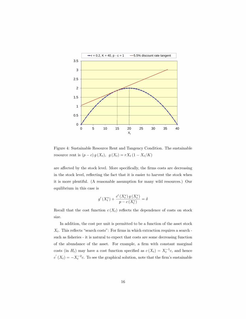
r = 0.2, K = 40, p - c = 1 5.5% discount rate tangent

Figure 4: Sustainable Resource Rent and Tangency Condition. The sustainable

resource rent is (p− c) g (Xt), g (Xt) = rXt (1−Xt/K)

are affected by the stock level. More specifically, the firms costs are decreasing

in the stock level, reflecting the fact that it is easier to harvest the stock when

it is more plentiful. (A reasonable assumption for many wild resources.) Our

equilibrium in this case is

g0 (X∗t ) +c0 (X∗t ) g (X

∗t )

p− c (X∗t )= δ

Recall that the cost function c (Xt) reflects the dependence of costs on stock

size.

In addition, the cost per unit is permitted to be a function of the asset stock

Xt. This reflects “search costs”: For firms in which extraction requires a search -

such as fisheries - it is natural to expect that costs are some decreasing function

of the abundance of the asset. For example, a firm with constant marginal

costs (in Ht) may have a cost function specified as c (Xt) = X−1t c, and hence

c0(Xt) = −X−2t c. To see the graphical solution, note that the firm’s sustainable

16

-4

-3

-2

-1

0

1

2

3

4

5

6

0 5 10 15 20 25 30 35 40

Xt

r = 0.2, K = 40, p = 3, c = 20 5.5% discount rate tangent

Figure 5: Sustainable Resource Rent and Tangency Condition. The sustainable

resource rent is (p− c) g (Xt), g (Xt) = rXt (1−Xt/K), c (Xt) = cX−1t

resource rent for a given stock level Xt is

(p− c (Xt)) g (Xt) =

µp− c

Xt

¶rXt

µ1− Xt

K

¶so that the solution is simply given by the point where this function has slope

equal to δ. See figure 5.

The introduction of search costs pushes the optimal stock level to the right,

simply because due to the reduction in cost by doing so. If the search costs are

sufficiently great, and the discount rate sufficiently low, the optimal stock level

can be to the right of the maximum sustainable yield, as occurs in this example.

(Note that the MSY for the growth function in the example in the figure is 20.)

This is because the effect of search costs outweighs the effect of discounting in

this particular example.

17

2.2 Transition to equilibrium.

Although we have solved for the asset level and extraction rate in equilibrium for

our general model, we have not yet discussed how the transition to equilibrium

occurs.

When the profit function is linear in Ht, the firm simply stops extraction or

extracts the required amount to get to X∗t as fast as possible. This would be the

case for price-taking firms with constant marginal cost, or in general firms with

profit functions linear in Ht. The extraction rate Ht is said to be a switching

function, where

Ht =

⎧⎨⎩ 0 if Xt < X∗t

Hmax if Xt > X∗t.

Ht obeying the above insures that the equilibrium stock level is reached as fast

as possible (c.f. eq. (2.46) in Clark, 2010).

However, if the owner has market power, then as the supply is restricted

to conserve and grow the asset base, the price is driven up. At some point,

the price reaches such a level that it becomes optimal for the owner to extract.

Thus under market power - and in more general cases where the profit function

is non-linear in Ht - there is a smooth transition to the optimal stock level. This

smooth transition can be solved for recursively, by solving backwards from the

equilibrium conditions. In general this recursion is dependent on key parameters

governing cost and price that will be unobservable to the economist. However,

because the assumption of market power is untenable for many of the firms we

are considering, we will not pursue this solution any further. We refer the reader

to chapter 4 of Clark (1985) for a more detailed explanation of how the optimal

transition path can be derived in a more complicated model with market power.

Smooth transition may also occur if there are search costs. As the asset stock

is conserved, the marginal cost of extraction decreases, and again at some point

it becomes optimal to extract. However, as stated above, due to both the lack

of empirical and theoretical relevance of search costs and the complications it

would create for valuation, we shall continue to maintain zero search costs.

18

2.3 Separation of Asset Owner and Extracting Firm

The dynamic optimization problem has thus far only considered the case in

which the extracting firm has exclusive property rights to harvest the asset stock.

The only influence on the stock level is the firm’s own extraction, and hence

the firm only takes into account its own extraction when solving the dynamic

optimization problem. This precludes cases in which other factors that are not

under the control of the firm can affect the stock level. In particular it precludes

the case in which other firms are harvesting the stock.

In practice for many wild biological resources no single firm has exclusive

rights to harvest. In this case, the effect of any single given firm’s extraction

rate on the growth of the asset becomes diluted as the number of firms accessing

the asset increases. For a large enough number of firms, each firm will disregard

its own extraction rate when optimizing future profits,and each firm will also

disregard the extraction rate of other firms. (In practice this situation closely

corresponds to unregulated wild resources, whereby any firm can enter and har-

vest the stock.) In this case the dynamic aspect of the optimization problem

disappears, and the firm simply selects the harvest rate at which marginal cost

equals marginal revenue. The value of the stock can then be derived under

this so-called “open access” situation given the growth function of the stock.

Typically the asset value is far below that in the case where a single firm has

exclusive property rights. In many cases the wild resource is harvested until

it disappears. However, open access is becoming increasingly scarce as govern-

ments act to preserve wild resources. Typically this is achieved by the regulator

(henceforth “owner”) limiting the amount harvested over a given period.

In this subsection we consider the case in which the owner of the stock

distributes rights to harvest to extracting firms in each period. The owner

manages the sequence of harvests according to some objective function, and

under the assumption that the harvesting rights are exhausted once distributed

(that is, the extractor does not harvest any less than he is permitted). We will

consider the case of a continuum of competing firms, so that the individual firm

does not consider the impact of its harvest on the growth rate of the asset, nor

does it interact strategically with other firms when choosing its own extraction

19

rate. Instead, we assume that a regulator sets totalHt according to her objective

function, before allocating out individual extraction rights hi,t to various firms

i = 1, ...., n, subject to Ht =Pn

i=1 hi,t. Obviously we must make an assumption

about the regulator’s objective function.

When the resource manager has a stated extraction policy, the best op-

tion may be to use the stated policy to determine the asset value regardless of

whether the stated policy is economically optimal. In the example given in the

following section, the resource manager explicitly states its control policy for

Ht as a function of the underlying stock size Xt, so that we can directly predict

how Ht will change over time (given of course some growth function.) Often

these so-called “reference point” strategies are set without regard to optimiz-

ing the value of the asset, but are rather ad-hoc rules for managing the stock

to a stock level somewhere in the vicinity of Xmsy (Hilborn, 2002). Typically

these reference point rules are linear functions of the underlying stock level. For

example, a linear reference point rule is as follows.

Ht =

⎧⎪⎪⎨⎪⎪⎩0 if Xt ≤ a

(b− a)−1 (Hmax − a) if a < Xt ≤ b

Hmax if Xt > b

Note that under this reference point rule, if b = Xmsy, then for all Xt > Xmsy

there is unrestricted extraction of the asset. In this way convergence to the

steady state may not be smooth, let alone be achieved at all. Another reference

point rule that ensures convergence to Xmsy is as follows.

Ht =

⎧⎪⎪⎨⎪⎪⎩0 if Xt ≤ a

(b− a)−1 (Hmsy − a) if a < Xt ≤ b

Hmsy if Xt > b

(10)

Although this rule does not maximize the asset value, it does ensure smooth

convergence to Xmsy.

In the absence of a stated policy, the economist must make an assumption

about the regulator’s objective function. In such situations we may wish to

assume that the regulator’s goal is to maximize firm profits, and has knowledge

of the costs and market structure for the good in question. Such an assumption

may rightly be perceived as heroic. Yet we require an assumption about the

20

objective function of the agent controlling the asset, and in the absence of a

better assumption, we will assume that the regulator has profit maximization

as her primary goal. In this case, she chooses H∗t according to (6) and (7).

3 Application.

In this section we use biological and accounting data provided by the National

Oceanic and Atmospheric Administration (NOAA) in order to value an Alaskan

crab fishery. NOAA provides estimates of stock levels, catch levels, Hmsy and

Xmsy as well as reference points rules (10) for determination of the fishing quotas

(“total allowable catch”). NOAA also provides limited accounting data on the

costs and revenues realized by firms harvesting the crabs.

NOAA conducts surveys of many wild fish stock populations, but economic

data associated with these stocks is lacking. However, recipients of fishing quo-

tas in the Alaskan King Crab fishery are required to fill out economic surveys

administered by the NOAA. These surveys cover the revenues from Alaskan

crab harvesting, and a substantial proportion of the costs. On the cost side,

gasoline and capital costs are omitted from the survey. The 2010 Stock Assess-

ment and Fishery Evaluation (SAFE) report contains this limited accounting

survey data for the Alaskan Crab fisheries. The SAFE surveys are issued on

an annual basis, but SAFEs previous to 2010 typically only contain data on

harvests and stock levels. In what follows, we will combine the accounting data

from the 2010 SAFE with biomass data from the 2009 SAFE into a working

example for valuation of near-market assets under endogenous growth.

All data are at an annual frequency. Typically, the fleet harvests several

species of crab across a given year. The most harvested are the Bristol Bay Red

King crab, Opilio (Snow) crab, and the Tanner crab. We will value these three

stocks jointly, because some of the costs from the 2010 SAFE report are not

allocated to the harvesting of each species.

21

3.1 Growth function.

NOAA publishes detailed data on the stock levels for the Alaskan King crab,

Tanner crab and Opilio (“Snow”) crab stocks together with estimates of the

Hmsy and Xmsy. From this we can identify a two-parameter growth function,

such as the logistic function. NOAA also publishes past data on Total Allow-

able Catch (TAC) and realized catches for the fisheries. They also publish their

stated reference point rules for determining future TACs. Given a growth func-

tion, from this data we can infer the future growth in the asset stock and TAC

under NOAA’s stated reference point rules for extraction of the stock to bring

the stock level toXmsy. Tables 1 to 3 below give the past and predicted managed

changes in three crab stocks located in the Bering Sea.

Table 1: Projected Harvests and Stocks (millions lbs)

Bristol Bay Red King Crab

Xmsy Hmsy Xt Ht gl (Xt)

2005 80 18

2006 82 16

2007 86 20

2008 75.1 24.2 95.6 20.4 22.4

2009 75.1 24.2 97.6 24.2 22.0

2010 75.1 24.2 95.5 24.2 22.4

2011 75.1 24.2 93.7 24.2 22.7

2012 75.1 24.2 92.2 24.2 22.9

2013 75.1 24.2 90.9 24.2 23.1

2014 75.1 24.2 89.9 24.2 23.3

2015 75.1 24.2 88.9 24.2 23.4

2020 75.1 24.2 85.6 24.2 23.7

2030 75.1 24.2 82.3 24.2 24.0

Entries in bold denote historical data obtained from the 2009 SAFE. Here Ht

denotes the annual harvest and Xt denotes the stock level at the start of the season.

Entries in standard font denote estimates for the maximum sustainable yield Hmsy

22

and the MSY stock level Xmsy and are obtained from the 2009 SAFE. Numbers in

italics represent our projections using harvest rates Ht prescribed by the stated

reference point rules from the 2009 SAFE and growth in stock levels using the

logistic growth function gl (Xt). The reference point rule used by NOAA for the

King Crab is Ht = Hmsy because Xt > Xmsy. The stated years refer to the year in

which the fishing season begins; e.g. “2008” refers to the 2008-2009 fishing season.

Note that projected extraction rates are set equal to the Hmsy for the King

crab stock. This is because stock levels in 2008 exceed the maximum sustainable

yield stock level. Thus going forward it is assumed that the TAC in each season

will be set equal to the estimated Hmsy = 24.2. (This is in accordance with

the stated reference point rules of NOAA in the 2009 SAFE.) We can see that

as time passes the stock level is forecasted to approach the Xmsy = 75.1 rather

slowly.

Table 2: Projected Harvests and Stocks (millions lbs)

Bering Strait Tanner Crab

Xmsy Hmsy Xt Ht gl (Xt)

2005 86.2 4.2

2006 126.6 12.0

2007 150.7 8.8

2008 189.6 26.7 118.2 5.0 22.9

2009 189.6 26.7 136.2 18.3 24.6

2010 189.6 26.7 142.4 19.3 25.0

2011 189.6 26.7 148.1 20.2 25.4

2012 189.6 26.7 153.3 21.0 25.7

2013 189.6 26.7 158.0 21.7 25.9

2014 189.6 26.7 162.2 22.4 26.1

2015 189.6 26.7 165.9 23.0 26.3

2020 189.6 26.7 178.7 25.0 26.6

2030 189.6 26.7 187.5 26.3 26.7

23

See note to table 1 above. The reference point rule used by NOAA for the Tanner

Crab is Ht = Hmsy (Xt/Xmsy − 0.1) /0.9.

Table 3: Projected Harvests and Stocks (millions lbs)

Bering Strait Snow Crab

Xmsy Hmsy Xt Ht gl (Xt)

2005 188.0 46.9

2006 218.0 49.4

2007 218.0 78.6

2008 317.7 101.9 241.0 69.5 96.0

2009 317.7 101.9 267.5 85.8 99.4

2010 317.7 101.9 281.0 90.1 100.5

2011 317.7 101.9 291.4 93.5 101.2

2012 317.7 101.9 299.2 96.0 101.6

2013 317.7 101.9 304.8 97.8 101.7

2014 317.7 101.9 308.7 99.0 101.8

2015 317.7 101.9 311.5 99.9 101.9

2020 317.7 101.9 316.8 101.6 101.9

2030 317.7 101.9 317.7 101.9 101.9

See note to table 1 above. The reference point rule used by NOAA for the Snow

Crab is Ht = Hmsy (Xt/Xmsy − 0.1) /0.9.

Note that while the King crab stocks were above their maximum sustain-

able yield biomass in 2008, the Snow and Tanner crab stocks were below their

corresponding MSY biomass levels. For these two crab stocks, the reference

point transition function applied by NOAA prescribes a harvesting rate that

approaches the MSY from below. As time passes the projected harvest ap-

poaches Hmsy, with the Hmsy being reached by 2030 for both the Snow and

Tanner crab stocks. This demonstrates the importance of knowing where the

current stock level is in relation to the maximum sustainable yield stock level is

when projecting the harvesting rates into the future.

24

3.2 Valuation.

Tables 4 and 5 below summarize the economic data for the entire crab fishery.

Note that we impute a gasoline cost using average fuel prices in Alaska. The Red

King crab, Tanner crab and Snow crab fisheries exhibit substantial variation in

revenue over the period. This is more due to volatility in the price received per

25

pound of crab over the time period rather than from changes in volume of catch.

Table 4: Revenue and Costs for Alaskan Crab Fisheries

revenue labor bait observer costs gas avg. return

Year mil $ mil $ mil $ mil $ mil $ mil $

Bristol Bay Red King Crab

1998 42.38 9.38 1.17 0.03 n/a n/a

2001 45.57 9.83 0.96 0.16 n/a n/a

2004 78.35 17.31 1.32 0.02 n/a n/a

2005 84.87 11.16 0.75 0.00 25.70 47.26

2006 60.95 8.17 0.59 0.00 23.08 29.11

2007 87.84 11.03 0.77 0.00 30.94 45.10

2008 96.97 13.15 0.98 0.00 48.04 34.80

Bering Strait Snow Crab

1998 150.13 33.77 4.28 0.12 n/a n/a

2001 39.27 7.91 1.33 0.05 n/a n/a

2004 54.33 11.68 1.18 0.06 n/a n/a

2005 46.24 10.00 0.94 0.04 30.88 4.38

2006 39.90 5.66 0.54 0.00 38.25 -4.55

2007 56.74 8.34 0.45 0.00 31.58 16.37

2008 98.41 14.60 0.65 0.00 68.82 14.35

Bering Strait Tanner Crab

1998 — — — n/a n/a n/a

2001 0.03 0.00 0.00 n/a n/a n/a

2004 — — — n/a n/a n/a

2005 0.44 0.05 0.01 0.01 0.09 0.35

2006 1.44 0.22 0.02 0.00 0.54 0.90

2007 3.99 0.58 0.08 0.00 0.76 3.23

2008 4.04 2.73 0.12 0.00 1.09 2.95

“Observer costs” refer to the costs associated with monitoring of fishing practices by

the regulator. Data obtained from the 2010 SAFE.

26

Table 5: Costs for all Alaskan Crab Fisheries

Taxes Co-op Freight Storage Gear Pots Repairs Capital

fees Invst.

mil $ mil $ mil $ mil $ mil $ mil $ mil $ mil $

Additional Costs: All Fisheries

1998 4.19 n/a 0.01 1.53 3.49 3.97 0.02 22.47

2001 1.94 n/a n/a 1.23 1.80 0.96 0.02 13.26

2004 2.84 n/a n/a 1.53 1.93 0.95 0.02 17.88

2005 5.27 0.28 0.00 0.96 0.84 0.69 0.00 0.55

2006 5.92 0.47 0.00 0.54 0.91 0.54 0.00 0.55

2007 9.50 0.82 0.00 0.59 0.73 0.37 0.00 1.87

2008 13.46 0.56 0.00 0.87 1.28 0.53 0.00 0.68

Data obtained from the 2010 SAFE. Note that 2008 refers to the 2008-2009 fishing

season.

We thus have data on the average profitability of the crab fishery. As stated

under the previous subsection, under the assumption of perfect competition,

constant marginal cost, and no search costs, average profit is equal to marginal

profit per unit. We can use the projected growth in the harvest - given in tables

1 to 3 - to back out an estimate of the profitability of the fishery. We assume all

costs per unit and revenues per unit are the same as in the 2008 season. Then

using the discount factor δ, we can calculate the net present value of the fishery.

In doing so, we omit taxes from the fixed costs. That is, the valuation of the

crab stock at time 0 is given by

V0 =∞Pt=1

µ1

1 + δ

¶t(Hking

t πking +Htannert πtanner +Hsnow

t πsnow − C)

where πking denotes the per-lb profit of the red king crab in 2008, and Hkingt

denotes the projected harvest rates of the king crab at time t, etc., and C

denotes the costs given in table 5 that cannot be attributed to a single crab

stock.

27

Note the similarity to the valuation equation (1) above. Here, however, we

are working in discrete time. The discount factor (1 + δ)−t corresponds to e−δt

in (1). In our example only the King Crab stock is being harvested at the

MSY level; for the remaining stocks, the annual harvest increases over time as

the stock level is built back up to the MSY level. But because we have the

harvesting policy of the regulator, we can project future harvests Ht once we

have made an assumption about the growth function g (Xt). Last, because of

our assumptions on market and firm structure, the marginal profit per unit is

expected to remain constant. That is p (Ht)− c (Xt,Ht) in (1) is constant.

Table six gives the valuations for various discount factors δ.

Table 6: Bering Sea Crabs

Valuation in current $ (mil)

δ = 0.04 δ = 0.07 δ = 0.1

1,704.299 973.605 678.756

Table 6 demonstrates that the choice of discount rate has a large impact

on the value of the asset. Increasing the discount rate from 4% to 10% more

than halves the value. As discussed earlier, in practice the determination of the

appropriate discount rate is an important task. Reporting valuations for a range

of discount rates may also be desirable in order to reflect the sensitivity of the

analysis to key model parameters. To put the range of valuations in context,

the total revenue from the Alaskan “Fisheries, Forestry and related” NAICS

industry was $316 million in 2008.

Note that capital costs have been excluded from all calculations. A final

step would be to subtract the value of the capital used in extraction - namely

the fleet of boats - from the stated value of the fishery above. As this data is

lacking, we do not take his final step, and instead treat the figures given in the

table above as a joint valuation of the fishery and fleets together.

28

4 Conclusion.

This paper summarizes the extant literature on bioeconomics. Our specific focus

is outlining the necessary assumptions that permit valuation of near-market

assets based on the average profits obtained from the asset. It is shown that for

resources that have a single owner, perfect competition, constant marginal cost,

and independence of costs from asset abundance are sufficient assumptions on

the economic side for valuation. On the biological side, it is necessary to make

an assumption of the growth function of the asset.

We apply the valuation methods to a specific US crab fishery, but the meth-

ods can be applied to a wider range of assets that grow endogenously, such as

other fishery species, forestry, agriculture and horticulture. We found that the

valuation of the crab fishery is not robust to changes in the discount rate.

5 Appendix: Classic Hotelling Valuation

In the conventional Hotelling framework the amount of the asset Xt is finite.

Hence our maximization constraint becomes

∂Xt

∂t= −Ht,

Z ∞0

Htdt = X0

Now for the price-taker with constant marginal cost, we have π (Ht,Xt) =

(pt − ct)Ht, where ct is a constant marginal cost. The solution is as follows.

The present value Hamiltonian is

L (Ht,Xt, ψ) = e−δtπ (Ht,Xt)− λHt

Then the FOCS are

∂L (Ht,Xt, ψ)

∂Ht= 0 =⇒ e−δt (pt − ct) = λt

∂L (Ht,Xt, ψ)

∂Xt= −λt =⇒ λt = 0

so λt = λ is constant. Solving out we have e−δt (pt − ct) = λ, which implies

that pt − ct = eδt (p0 − c0). Then the value asset is

V0 =

Z ∞0

e−δteδt (p0 − c0)Htdt = (p0 − c0)

Z ∞0

Htdt = (p0 − c0)X0

29

sinceR∞0

Htdt = X0, which is the classic Hotelling valuation principle.

References

[1] Alvarez, Antonio, and Peter Schmidt. "Is Skill More Important Than Luck

In Explaining Fish Catches?." Journal Of Productivity Analysis 26.1

(2006): 15-25.

[2] Clark, Colin W. (1985) “Mathematical Bioeconomics,” John Wiley & Sons,

Inc., Hoboken, New Jersey.

[3] Clark, Colin W. (2010) “Mathematical Bioeconomics,” John Wiley & Sons,

Inc., Hoboken, New Jersey.

[4] Clarke, H and Reed, W. J. (1989) “The Tree cutting problem in a stochas-

tic environment: The Case of Age-Dependent Growth” Journal of Eco-

nomic Dynamics and Control 13, 569-595.

[5] Cochrane, J. (2010). “Discount Rates”. NBER Working Paper No. 16972

[6] Crutchfield, J.A. and A. Zellner. 1962. Economic Aspects of the Pacific

Halibut Fishery, Fishery Industrial Research, vol. 1, No. 1, Washington,

US Department of Interior

[7] Fretwell, S. D., and H. L. J. Lucas.(1970) “On territorial behavior factors

influencing habitat distribution in birds.” Acta Biotheor., (19) 16-36.

[8] Gordon, H.S. (1954), “The economic theory of a common property resource:

the fishery,” Journal of Political Economy, 62, 124-142.

[9] Gordon, M. (1992), “Mathematical bioeconomics and the evolution of mod-

ern fisheries economics”, Bulletin of Mathematical Biology, vol. 54 no.

27, 163-184.

[10] Herrero, Ines, Sean Pascoe, and Simon Mardle. "Mix Efficiency In A Multi-

Species Fishery." Journal Of Productivity Analysis 25.3 (2006): 231-

241.

[11] Hilborn, R. (2002) “The dark side of reference points.” Bulletin of Marine

Science, March, 403-408.

30

[12] Hotelling, H (1931) “The Economics of Exhaustible Resources” Journal of

Political Economy 39, 137-75

[13] Kirkley, James, Dale Squires, and Ivar E. Strand. "Characterizing Manage-

rial Skill And Technical Efficiency In A Fishery." Journal Of Produc-

tivity Analysis 9.2 (1998): 145-160

[14] Kompas, Tom and Che, Tuong Nhu. "Efficiency Gains And Cost Reduc-

tions From Individual Transferable Quotas: A Stochastic Cost Frontier

For The Australian South East Fishery." Journal Of Productivity Anal-

ysis 23.3 (2005): 285-307.

[15] Miller, M. H. and Upton, C. W. (1985) “A Test of the Hotelling Valuation

Principle” The Journal of Political Economy 93, 1—25.

[16] National Oceanic and Atmospheric Administration (2009) “Stock Assess-

ment and Fishery Evaluation Report for the King and Tanner Crab

Fisheries of the Bering Sea and Aleutian Islands Regions.”

[17] National Oceanic and Atmospheric Administration (2010) “Stock Assess-

ment and Fishery Evaluation Report for the King and Tanner Crab

Fisheries of the Bering Sea and Aleutian Islands Regions.”

[18] Nordhaus, W. D. (1997). “Discounting in Economics and Climate Change,”

Climatic Change 37, 315—328.

[19] Nordhaus, W. D. (2007). “A Review of the Stern Review on the Economics

of Climate”. Journal of Economic Literature 45 (3): 686—702.

[20] Nordhaus, William D., and Kokkelenberg, Edward C., (1999). Nature’s

Numbers: Expanding the National Economic Accounts to Include the

Environment. National Academy Press, Washington, DC.

[21] Scott, A. (1954), “Conservation policy and capital theory,” Canadian Jour-

nal of Economics and Political Science, 20, 504-513.

[22] Stern, N. (2006) “Stern Review on the Eco-

nomics of Climate Change”, available at

http://webarchive.nationalarchives.gov.uk/+/http://www.hm-

treasury.gov.uk/sternreview_index.htm

31

[23] Turvey, R. (1964), “Optimization and suboptimization in fishery regula-

tion,” American Economic Review, 54, 64-76.

[24] U.S. Bureau of Economic Analysis. (1994a). “Integrated Economic and En-

vironmental Satellite Accounts.” Survey of Current Business, 74(4), 33-

49.

[25] U.S. Bureau of Economic Analysis. (1994b). “Accounting for Mineral Re-

sources: Issues and BEA’s Initial Estimates.” Survey of Current Busi-

ness, 74(4), 50-72.

32