Valuation of Inflation-IndexedDerivatives with three factor model

Laura Malvaez

Keble College

University of Oxford

A thesis submitted for the degree of

Msc. in Mathematical Modelling and Scientific Computing

Trinity 2005

One must learn by doing the thing,

for though you think you know it,

you have no certainty until you try.

Aristotle.

This thesis is dedicated to

my parents and my sister

for all their support, love and care.

Acknowledgements

This work was supported by Sociedad Hipotecaria Federal, S.N.C. a mortgage bank in

Mexico, through their sponsorship for professional development for employees during

2004-2005.

I am grateful to Dr. Sam Howison and Dr. Henrik Rasmussen for their helpful guidance

and comments for the elaboration of this thesis.

I would like to express my thanks to Alan Elizondo and Ramon Montenegro for the

discussions which helped me develop the ideas put forward here, and other colleagues in

SHF who assisted in gathering the data used for the analysis.

Other friends whose comments and criticism I made use of include Andrea Schnepf, Tino

Wendish, Lucy Fernandez and Salvador Venegas.

Contents

1 Introduction 1

1.1 Inflation . . . . . . . . . . . . . . . . . . . . . . . . . . . . . . . . . . . . . . . . . . . 2

1.2 Inflation-indexed securities . . . . . . . . . . . . . . . . . . . . . . . . . . . . . . . . . 3

1.2.1 Nominal Rates, Real Rates and Expected Inflation . . . . . . . . . . . . . . . 5

1.3 Inflation-indexed derivatives . . . . . . . . . . . . . . . . . . . . . . . . . . . . . . . . 6

1.3.1 Examples of Inflation-liked payout structures . . . . . . . . . . . . . . . . . . 7

1.3.2 Use of swaptions for hedging Mortgage backed securities portfolios . . . . . . 8

2 Pricing of Derivatives 10

2.1 The Martingale approach . . . . . . . . . . . . . . . . . . . . . . . . . . . . . . . . . 10

2.1.1 Martingale Pricing . . . . . . . . . . . . . . . . . . . . . . . . . . . . . . . . . 11

2.2 Heath-Jarrow-Morton Framework (HJM) . . . . . . . . . . . . . . . . . . . . . . . . 13

2.2.1 Extended Vasicek Model . . . . . . . . . . . . . . . . . . . . . . . . . . . . . . 14

2.3 Notation . . . . . . . . . . . . . . . . . . . . . . . . . . . . . . . . . . . . . . . . . . . 15

2.4 Models for pricing Inflation-Indexed derivatives . . . . . . . . . . . . . . . . . . . . . 16

2.4.1 Jarrow and Yildrim Model (2003) . . . . . . . . . . . . . . . . . . . . . . . . 16

2.4.2 Fabio Mercurio Market Model (2004) . . . . . . . . . . . . . . . . . . . . . . . 18

2.4.3 Belgrade-Benhamou-Koehler Market Model (2004) . . . . . . . . . . . . . . . 19

3 Pricing derivatives using Jarrow and Yildrim 21

3.1 Pricing formulas for basic inflation swaps . . . . . . . . . . . . . . . . . . . . . . . . 21

3.1.1 Zero-coupon swap . . . . . . . . . . . . . . . . . . . . . . . . . . . . . . . . . 21

3.1.2 Year-on-year Swap . . . . . . . . . . . . . . . . . . . . . . . . . . . . . . . . . 22

3.2 Pricing a fixed real vs. floating nominal swap . . . . . . . . . . . . . . . . . . . . . . 24

3.3 Pricing European swaption . . . . . . . . . . . . . . . . . . . . . . . . . . . . . . . . 26

i

4 Estimation of parameters and Valuation using quasi-Monte Carlo Simulation 29

4.1 Mexican Inflation Linked market . . . . . . . . . . . . . . . . . . . . . . . . . . . . . 29

4.1.1 Estimating parameters for nominal and real markets . . . . . . . . . . . . . . 29

4.1.2 Estimation of parameters of Inflation . . . . . . . . . . . . . . . . . . . . . . . 31

4.1.3 The effect of seasonality of inflation in option pricing . . . . . . . . . . . . . . 32

4.2 Quasi-Monte Carlo simulation . . . . . . . . . . . . . . . . . . . . . . . . . . . . . . . 33

4.2.1 Quasi-Random Numbers: Faure Sequence . . . . . . . . . . . . . . . . . . . . 33

4.2.2 Generating Multivariate Normal Variables . . . . . . . . . . . . . . . . . . . . 34

4.2.3 Analysis of Results . . . . . . . . . . . . . . . . . . . . . . . . . . . . . . . . . 35

5 Bermudan Swaption 38

5.1 Longstaff and Schwartz Approach . . . . . . . . . . . . . . . . . . . . . . . . . . . . . 38

5.1.1 Valuation framework . . . . . . . . . . . . . . . . . . . . . . . . . . . . . . . . 38

5.1.2 Least-Square Monte Carlo for Bermudan Swaption . . . . . . . . . . . . . . . 41

6 Conclusion 43

A Glossary 46

B Analysis of Historical Data 48

C Analysis of Results 50

D Example Faure sequences 58

D.1 The inverse cumulative normal function . . . . . . . . . . . . . . . . . . . . . . . . . 60

Bibliography 61

ii

Chapter 1

Introduction

In a world facing an aging population, the priorities of investors are changing. The investors saving

for their retirement are interested in sacrificing current spending for future consumption, only if

the real worth of their money is guaranteed. The uncertainty of future inflation and its effect in

the reduction of acquiring power is one of the driving forces that is boosting the inflation indexed

markets.

Inflation-indexed derivatives are a relatively new class of instruments in the global financial

markets. Their characteristics resemble those of the interest rate and foreign exchange derivatives.

In the past ten years, the inflation-indexed market has risen steadily in Euro-zone and in other

countries where there is an inflation-indexed securities market. The big investment banks and

financial firms still consider it as having a large potential market growth worldwide.

The main objective of this thesis is to implement a non-arbitrage model for pricing inflation-

indexed derivatives, specifically inflation-indexed swaptions in their European and Bermudan ver-

sion. In the first chapter, an introduction of inflation-related concepts is presented together with the

main motivation to research this topic. The second chapter presents an overview of the theoretical

background necessary to develop the model used for option pricing. It is worth mentioning that the

model presented is suitable for a market where some inflation-indexed securities are traded1, but

where there is not a liquid market for inflation-indexed derivatives. At the end of this chapter, a

review of two more complex models is presented as well as the reasons as why to they were not cho-

sen for implementation. In the third chapter the pricing formulas for some plain vanilla instruments

(swaps) are developed, focusing on the pricing of an European inflation-indexed swaption. Chapter

four focus on the implementation issues of the model, the estimation of parameters and analysis of

results for the European swaption. In the last chapter, we use the Longstaff and Schwartz model

for the pricing of a bermudan inflation-indexed swaption. Finally both conclusions and further

extensions of the work are presented.1It is possible to build term structure of real and nominal rates

1

To help this paper be a self contained work, there is a glossary with some key concepts or

financial “jargon” that were not defined in the body of the paper which I consider important for the

understanding of some of the theorems or explanations presented2.

1.1 Inflation

The first question that might arise is what is inflation and what causes it? Inflation can be defined

as a sustained increase in the general price level of goods across the economy, if the prices decrease

then it is called deflation. Inflation diminishes the acquiring power of the population in general.

To explain what causes inflation, economists have produced several theories using macroeconomic

and microeconomic analysis. One of the postulated underlying causes of inflation is the level of

monetary demand in the economy - how much money is being spent. Inflation tends to rise when, at

the current price level, demand for goods and services in the economy is greater than the economy’s

ability to produce them. Another factor that increases inflation is the expectation of it. Expected

inflation matters for wages and prices because future price rises reduce the amount of goods and

services that today’s wage settlement can buy. One of core purposes of the Central Banks is to

maintain stability of prices (i.e. low inflation) which they control through their monetary policy.

Expected inflation is affected by the monetary policy and how much people believe in the ability

and commitment of the authorities - the government and the central bank - to achieve their inflation

objectives.

Figure 1.1: UK CPI time series 1996-2005, CPI April 1996=100. Source: National Statistics UK

2We do not pretend to present an extensive glossary, therefore there might be concepts that are not defined andwas of interest of the reader to know their definition.

2

Consumer behaviour has seasonal features: for example consumption rises around Christmas,

followed by a period of price discounting in January; the demand of energy and warm clothing tends

to be higher in cold winter months than in the summer, and so on. To some extent, this causes

prices to fluctuate which is reflected in the consumer price indices.

In the past fifty years, most developed countries have experienced decreasing levels of inflation.

However we might be at a significant inflexion point in terms of anti-inflation policy. Deflation is

just as much of a social evil as inflation and it has changed global policy makers stance. The efforts

to avoid deflation also suggest that the political pressure for central banks to contain inflation has

temporarily reduced. The central bankers are being encouraged to take a more balanced view with

regards to the trade-off between inflation risks and growth. It is not certain that this change in

emphasis is going to be beneficial or not, but it is generating a higher uncertainty over price levels

in the next 10 years than the uncertainty in the past 10 years.

Inflation is measured in many ways. The most familiar measure in the UK is the Retail Prices

Index (RPI), but monetary policy is now based on the Consumer Prices Index ; (CPI) (See figure

1.1)). Both measure the prices of products and services that consumers buy. A price index is made

up of the prices of hundreds of goods and services - from basic items like bread to new products,

such as PCs. Prices are sampled up and down the country every month; in supermarkets, petrol

stations, travel agents, insurance companies and many other places. All these prices are combined

together to produce an overall index of prices. Inflation rate is then a measure of the average change

in prices across the economy over a specified period, most commonly 12 months. If, say, the annual

rate of inflation in January this year was 3%, then prices overall would be 3% higher than in January

last year. So a typical basket of goods and services costing, say, £100 last January would cost £103

this January.

The standard approach for modelling inflation is based on econometric models [11]. Their ob-

jective is to forecast inflation rate given a time series of data. Usually they relate inflation rate to

other macro economic variables such as short term interest rates and monetary policy and/or past

data of inflation (autoregressive models). The econometric approach nevertheless is not useful for

pricing derivatives. Econometric models are derived under the historical probability measure, while

the modern theory for option pricing requires the use of risk neutral probability which guarantees

the market is arbitrage free and the existence of a replicating hedging strategy3.

1.2 Inflation-indexed securities

Even in a stable low-inflationary environment, in the long term there remains a considerable uncer-

tainty about the real value of nominal bond returns, £100 now would have the purchasing power of

£74 in 30 years time if inflation averaged 1% but only £48 if inflation averaged 2.5%, more than3See Chapter 2 Martingale approach for option pricing.

3

50% less4. While an individual’s consumption basket might not change in the same proportion as

the change in the relevant inflation index, no other financial asset can give close to the real value

certainty of inflation-linked products.

Inflation-indexed securities are instruments that protect their buyers from changes in the general

level of prices in the economy. They guarantee that the security holder (buyer of the security) is

going to have the same purchasing power plus a fixed return. On the other hand, the borrower

(seller of security) is going to have a constant cost for their debt in real terms.

The use of indexed securities can be traced back as far as the 18th century when the state of

Massachusetts issued bills of public credit linked to the cost of silver [8]. The experience showed

that indexation based in one single good was not a good idea and more complex indexation methods

have been developed throughout history based on a basket of products that would reflect the prices

of the whole economy. It was until very recently (the second half of the 20th century) that indexed

debt became more popular in financial markets, particularly amongst governments after periods

of high and volatile inflation. For example countries in Latin America such as Argentina (1972-

1989), Brazil (1964) and Mexico (1989) have issued such securities as means of maintaining the

acceptability of long-term contracts. Countries with commitment to low inflation have made use of

indexed debt to lower their costs and to increase the credibility of their economic policies within

the markets. Recent issues include UK Gilt (1981), Australia CIBs (1985), Canada RRB (1991),

Sweden (1994), US TIPS (1997), France OATi (1998), Greece SBIL (2003) and Italy BTP(2003).

Most of the issuers of inflation-index securities are governments but corporations could also benefit

from it. Corporate balance sheets are full of real assets, so offsetting these with real liabilities could

be appealing. Large company cash flows also tend to have a considerable inflation element to them.

For instance, supermarkets sales will be similar to the inflation basket and so their prices will rise

in a similar vein. Some utilities and public infrastructure projects may have more direct inflation

linked revenues, which is strongly in their interest to hedge. Having inflation exposure hedged within

the portfolio of a corporate acts as a revenue stabiliser.

There are a large number of cash flow structures for inflation indexed securities, the most common

are capital indexed bond, interest indexed bond, current pay indexed, indexed annuity and indexed

zero-coupon bonds5.

Unique features of inflation bonds include their ability to provide low or negative return corre-

lation with other assets, long duration6 with respect to real interest rates, and low yield volatility.

Benefits (1)protect assets and future income against inflation (2)better match liabilities and assets

when both are affected by inflation (3)provide diversification in combination with other assets.

4The current inflation target of the Bank of England is 2% annually, the Mexican Central Bank inflation target is3.5% annually.

5For a description of structures Deacon et. al (2004) Chapter 2.6Look in the glossary for Duration.

4

According to the view of Barclays Capital [2], demographic pressures are such that it is quite

conceivable for the inflation-linked market to continue growing at its current rate. For instance, if

US pension funds were to allocate the same percentage of their assets to linkers as have UK pension

funds, this allocation would be larger than the current global market ($600bn). Even UK pension

funds have offset less than only a quarter of their total inflation-linked liabilities with inflation-linked

bonds. Japanese pension funds have a higher percentage of their liabilities with inflation linkages

and are further along the demographic transition but are only just starting to address this exposure.

In spite of its growth in the past years, this market is still young and as a consequence, has some

drawbacks such as lack of liquidity.

1.2.1 Nominal Rates, Real Rates and Expected Inflation

The yield on an inflation-indexed security represents the real return that the investor could realize by

holding the security to maturity. In nominal terms, the investor earns this real return plus additional

compensation for any inflation realized over the life of the security. By comparison, the total nominal

return realized by holding a nominal security to maturity is simply equal to its yield. That yield

embeds the return that the investor demands to compensate him for expected future inflation and

the risk associated with that inflation. An indexed security offers the investor protection against

unanticipated changes in inflation, while a nominal security does not.

In an environment of complete and efficient nominal and real debt markets, on any particular

day, the ex ante nominal and real rates are directly observable. If there are some investors in

both markets, the difference between nominal and real rates must reflect their expectation of future

inflation. Because investors might be compensated for bearing inflation risk, the yield on the nominal

security may include an inflation risk premium. If this risk premium is positive, as is often assumed,

inflation compensation will exceed the expected rate of inflation. In a world of deterministic interest

nominal and real rates, their difference is exactly equal to the certain inflation rate over the same

period.

The prices of real and nominal bonds not only depend on expectations of real and nominal

interest but also on tax regimes, market liquidity, the choice of index, the indexation method for

real bonds and so on. These factors are going to be ignored in this thesis in order to keep our model

simple and parsimonious.

There are a number of articles regarding the relationship between nominal and real rates, the

expectation of future inflation and inflation risk premium in several economies using the econometric

approach. For example: Sack (2000) [20] analyses US nominal and real yields and finds that the rate

of inflation expected over the next ten years fell from 3% in mid-1997 to 2.5% at the beginning of

2000. Deacon and Derry [7] described a number of techniques to produce an inflation a term structure

5

of from the UK government bonds. They concluded that their preferred was one developed by Arak

and Keicher which was used by Bank of England to produce its inflation report.

1.3 Inflation-indexed derivatives

The market for inflation-indexed or inflation-linked (IL) derivatives has grown considerably since its

beginning in the early 1990s, in countries like UK and Euro-zone. Derivatives are usually designed

and used to fill in the gaps and to produce synthetically complicated payoff structures that the

underlying market can not produce solely in order to fulfill the demand of issuers or investors. It is

not the exception with IL derivatives, they have added flexibility to the underlying inflation-indexed

bond markets and have opened up opportunities to achieve financial objectives unavailable through

the use of indexed-bonds solely. Their hedging capability against variety of risks is one of their

most appealing characteristics in reality: to match the timing and frequency of cash flows, index

matching, maturity matching among others.

The most common products traded nowadays are IL swaps (ILSs). Options (caps and floors),

swaptions and other derivatives have started trading in small amounts. They are likely to grow on

a more standardized basis, but are likely to develop in parallel with hedging requirements of the

end users (e.g. the currently trading in the UK market LPI7 swaps which are based on annual RPI

inflation but with a floor of 0% and a cap of 5%) rather than a replication of what trades in the

interest rate market8.

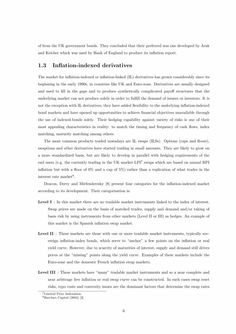
Deacon, Derry and Mirfenderesky [8] present four categories for the inflation-indexed market

according to its development. Their categorisation is:

Level I : In this market there are no tradable market instruments linked to the index of interest.

Swap prices are made on the basis of matched trades, supply and demand and/or taking of

basis risk by using instruments from other markets (Level II or III) as hedges. An example of

this market is the Spanish inflation swap market.

Level II : These markets are those with one or more tradable market instruments, typically sov-

ereign inflation-index bonds, which serve to “anchor” a few points on the inflation or real

yield curve. However, due to scarcity of maturities of interest, supply and demand still drives

prices at the “missing” points along the yield curve. Examples of these markets include the

Euro-zone and the domestic French inflation swap markets.

Level III : These markets have “many” tradable market instruments and so a near complete and

near arbitrage free inflation or real swap curve can be constructed. In such cases swap reset

risks, repo costs and convexity issues are the dominant factors that determine the swap rates7Limited Price Indexation.8Barclays Capital (2004) [2]

6

relative to the more liquid securities along the yield curve. Specific supply and demand in

the swap market becomes a secondary issue that more finely defines the inflation swap prices

within these bounds. The UK Retail Price Index (RPI) swap market falls into this category.

On the other hand, the US CPI swap market has full and liquid Treasury Inflation Protection

Securities (TIPS) curve but it is an early stage of development.

Level IV : This level is currently hypothetical because all the markets in the world fall into one of

the categories mentioned before, nevertheless it is expected to appear in the near future. This

market has reached a level of maturity, liquidity and stability analogous to the major nominal

interest rate swaps markets, such that inflation-indexed swaps trade int heir own right but

side-by-side with the inflation-indexed bonds. The ILSs would themselves be basic tradable

market instruments and their prices set independently of any underlying sovereign or other

index-linked bond market, and as a nominal counterparts.

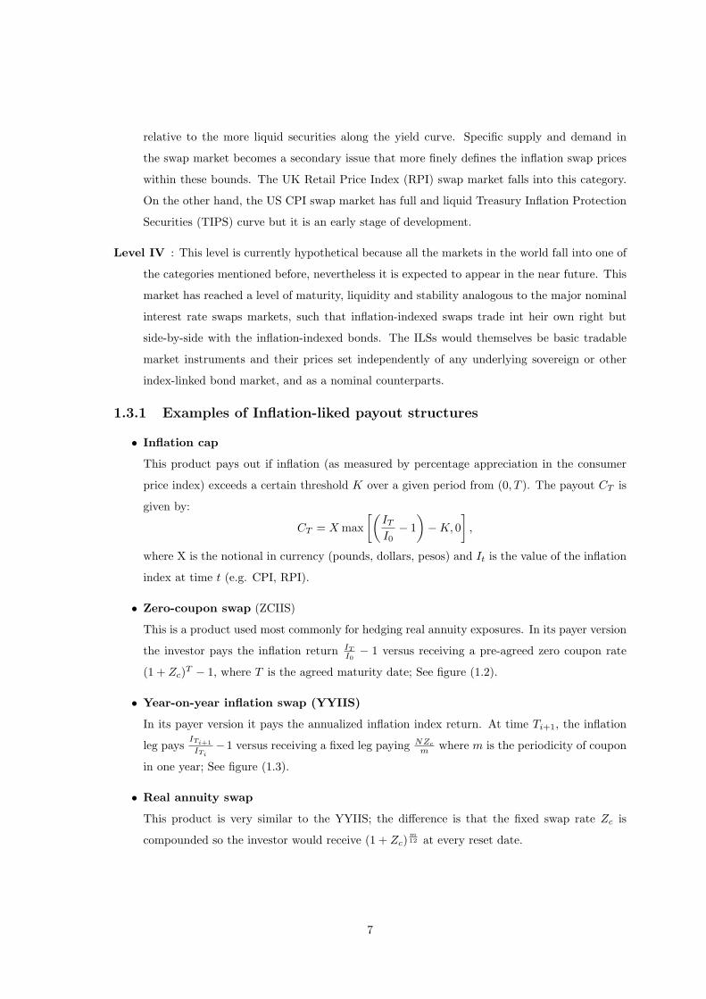
1.3.1 Examples of Inflation-liked payout structures

• Inflation cap

This product pays out if inflation (as measured by percentage appreciation in the consumer

price index) exceeds a certain threshold K over a given period from (0, T ). The payout CT is

given by:

CT = X max[(

IT

I0− 1

)−K, 0

],

where X is the notional in currency (pounds, dollars, pesos) and It is the value of the inflation

index at time t (e.g. CPI, RPI).

• Zero-coupon swap (ZCIIS)

This is a product used most commonly for hedging real annuity exposures. In its payer version

the investor pays the inflation return IT

I0− 1 versus receiving a pre-agreed zero coupon rate

(1 + Zc)T − 1, where T is the agreed maturity date; See figure (1.2).

• Year-on-year inflation swap (YYIIS)

In its payer version it pays the annualized inflation index return. At time Ti+1, the inflation

leg paysITi+1ITi

−1 versus receiving a fixed leg paying NZc

m where m is the periodicity of coupon

in one year; See figure (1.3).

• Real annuity swap

This product is very similar to the YYIIS; the difference is that the fixed swap rate Zc is

compounded so the investor would receive (1 + Zc)m12 at every reset date.

7

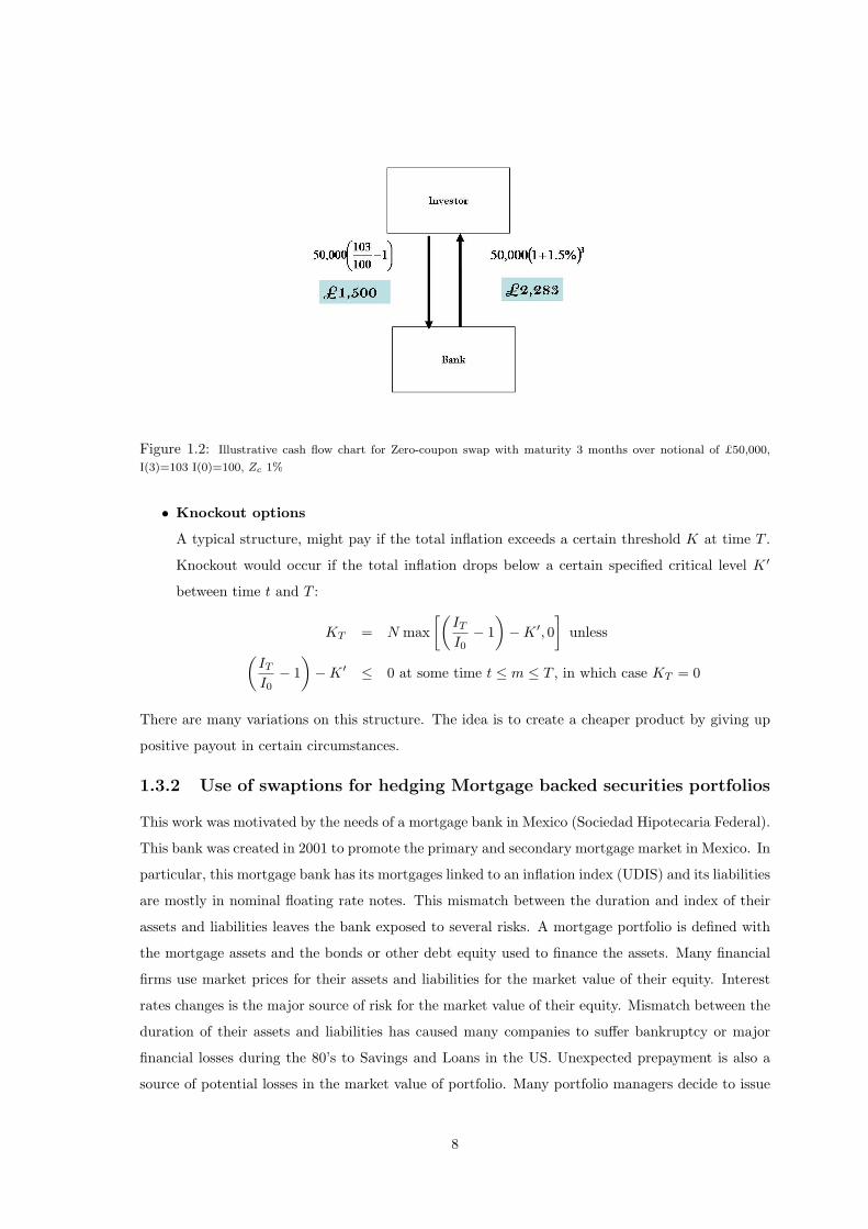
Figure 1.2: Illustrative cash flow chart for Zero-coupon swap with maturity 3 months over notional of £50,000,

I(3)=103 I(0)=100, Zc 1%

• Knockout options

A typical structure, might pay if the total inflation exceeds a certain threshold K at time T .

Knockout would occur if the total inflation drops below a certain specified critical level K ′

between time t and T :

KT = N max[(

IT

I0− 1

)−K ′, 0

]unless

(IT

I0− 1

)−K ′ ≤ 0 at some time t ≤ m ≤ T , in which case KT = 0

There are many variations on this structure. The idea is to create a cheaper product by giving up

positive payout in certain circumstances.

1.3.2 Use of swaptions for hedging Mortgage backed securities portfolios

This work was motivated by the needs of a mortgage bank in Mexico (Sociedad Hipotecaria Federal).

This bank was created in 2001 to promote the primary and secondary mortgage market in Mexico. In

particular, this mortgage bank has its mortgages linked to an inflation index (UDIS) and its liabilities

are mostly in nominal floating rate notes. This mismatch between the duration and index of their

assets and liabilities leaves the bank exposed to several risks. A mortgage portfolio is defined with

the mortgage assets and the bonds or other debt equity used to finance the assets. Many financial

firms use market prices for their assets and liabilities for the market value of their equity. Interest

rates changes is the major source of risk for the market value of their equity. Mismatch between the

duration of their assets and liabilities has caused many companies to suffer bankruptcy or major

financial losses during the 80’s to Savings and Loans in the US. Unexpected prepayment is also a

source of potential losses in the market value of portfolio. Many portfolio managers decide to issue

8

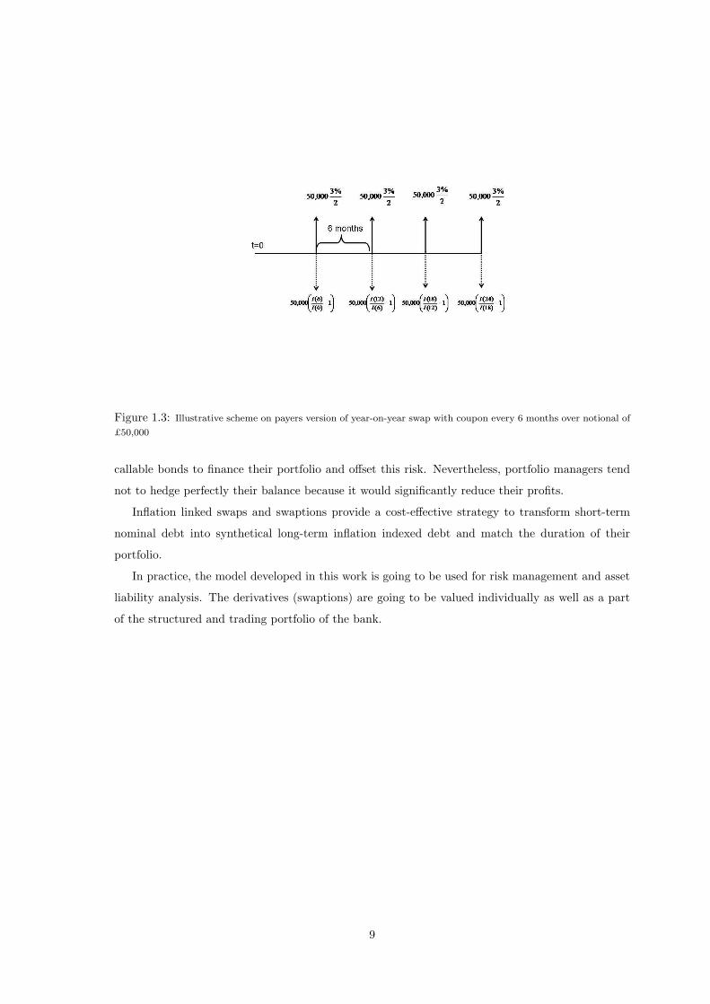
Figure 1.3: Illustrative scheme on payers version of year-on-year swap with coupon every 6 months over notional of

£50,000

callable bonds to finance their portfolio and offset this risk. Nevertheless, portfolio managers tend

not to hedge perfectly their balance because it would significantly reduce their profits.

Inflation linked swaps and swaptions provide a cost-effective strategy to transform short-term

nominal debt into synthetical long-term inflation indexed debt and match the duration of their

portfolio.

In practice, the model developed in this work is going to be used for risk management and asset

liability analysis. The derivatives (swaptions) are going to be valued individually as well as a part

of the structured and trading portfolio of the bank.

9

Chapter 2

Pricing of Derivatives

The first part of this chapter serves as introduction to martingale pricing established by Harrison and

Kreps and Harrison and Pliska, and a brief overview of the Heath Jarrow and Morton framework.

The second part of the chapter reviews the most popular models for pricing inflation-index derivatives

including some discussion about their assumptions and implementation suitability in a market with

characteristics of level II defined in Chapter 1.

2.1 The Martingale approach

Modern Financial theory has developed two fundamental theorems that state the conditions to

have an arbitrage free and complete market suitable for option pricing. Apart from their powerful

results they have allowed the development of very efficient computational implementations. The

mathematical proofs are going to be omitted due to their length and the requirement of deep results

from functional analysis1.

First we consider a market model consisting of the asset price processes S0, S1, ..., SN on the time

interval [0, T ]. The “numeraire process” S0 is assumed to be strictly positive.

Definition 2.1.1 A probability measure Q on FT is called an equivalent martingale measure for the

market model, the numeraire S0 and the time interval if it has the following properties:

• Q is equivalent2 to P on FT

• All price processes S0, S1, ..., SN are martingales under Q on the time interval [0, T ].

An equivalent martingale measure is often referred as “a martingale measure” or “an EMM”. If

Q ∼ P has the property that S0, S1, ..., SN are local martingales, then Q is called a local martingale

measure. The numeraire process S0 is always a martingale, and it is often referred as “the EMM”.1see Bjork [5, chapter 10 and 11]; he presents some of the proofs and further references.2A probability measure Q is equivalent to P if they have the same null sets, that is for all A ∈ F , Q(A) =

0 if and only if P (A) = 0.

10

The First Fundamental Theorem 2.1.1 The model is arbitrage free if and only if there exists a

martingale measure (Q ∼ P ) such that the processes

S0(t)S0(t)

,S1(t)S0(t)

, ...,SN (t)S0(t)

are (local) martingales under Q.

If the numeraire S0 is the money market account, i.e. dS0(t) = r(t)S0(t)dt, so that

S0(t) = B(t) = e−R t0 r(s)ds (2.1)

where r is the (possibly stochastic) short rate, and if we assume that all processes are Wiener driven,

then a measure Q ∼ P is a martingale measure if all assets have the short rate as their local rates

of return, i.e. the Q-dynamics are of the form

dSi(t) = Si(t)r(t)dt + Si(t)σi(t)dWQi (t) , i = 1, ..., N,

where WQ is a (multidimensional) Q-Wiener process.

Second Fundamental Theorem 2.1.2 Assuming absence of arbitrage, the market model is com-

plete if and only if the martingale measure Q is unique.

2.1.1 Martingale Pricing

If we want to price a contingent claim maturing at T given by X, first we consider the “primary”

market S0, ..., SN as given a priori. We have to determine a price process Π(t; X) for X assuming

that the primary market is arbitrage free. There are two main approaches:

• The derivative should be priced consistently with the prices of the underlying assets, i.e. the

extended market Π(·; X), S0, ..., SN is free of arbitrage.

• If the claim is attainable, with hedging portfolio h, then the only reasonable price is given by

Π(t,X) = V (t; h)

The first approach demands that there should exists a martingale measure for the extended market.

If we let Q as such measure, then the arbitrage free price process for the claim X is

Π(t;X) = S0(t)EQ

[X

S0(T )

∣∣∣Ft

]. (2.2)

where Q is the martingale measure for the a priori given market with S0 as numeraire. If we choose

the bank account B(t) as the numeraire equation (2.1) the pricing formula reduces to

Π(t; X) = EQ

[e−R T

tr(s)dsX

∣∣Ft

](2.3)

11

For the second approach we assume that X can be replicated by h. Since the holding of the derivative

contract and the holding of the replicating portfolio are equivalent, then the price of the derivative

must be given by

Π(t; X) = V (t;h)

in order to avoid arbitrage. Different choices of hedging portfolios (if such exist) will produce the

same price process.

There are two fundamental theorems that allow us to use the martingale approach to arbitrage

theory in a very simple way.

• The martingale representation theorem which shows that in a Wiener world every martingale

can be written as a stochastic integral with respect to the underlying Wiener process.

• Girsanov Theorem, which gives complete control of all absolutely continuous measure trans-

formations in a Wiener world.

The Martingale Representation Theorem 2.1.3 Let W be a d-dimensional Wiener process,

and assume that Ft is the filtration generated by the Wiener process Wt. Let M be any Ft-adapted

martingale. Then there exist uniquely determined Ft-adapted processes h1, ..., hd such that M has

the representation

M(t) = M(0) +i=1∑

d

∫ t

0

hi(s)dWi(s) , t ∈ [0, T ]. (2.4)

If the martingale M is square integrable, then h1, ..., hd are in H2.

The Girsanov Theorem 2.1.4 Let WP be a d-dimensional standard P -Wiener process on (Σ,P, P,F)

and let ϕ be any d-dimensional adapted column vector process. Choose a fixed T and define the

process L on [0, T ] by

dLt = ϕ∗t LtdWPt ,

L0 = 1,

i.e.

Lt = eR t0 ϕ∗sdW P

s − 12

R t0 ‖ϕs‖2ds.

Assume that

EP[LT ] = 1,

and define the new probability measure Q on FT by

LT =dQ

dP, on FT .

Then

dWPt = ϕtdt + dWQ

t ,

where WQ is a Q-Wiener process.

12

The process ϕ above will often be referred to as the Girsanov kernel of the measure transformation,

and is such that

EQ[e12

R T0 ‖ϕt‖2dt] < ∞;

L is called the likelihood function or the Radon-Nikodym derivative. An equivalent way (and more

popular) of formulating the conclusion of Girsanov’s Theorem is to say that the process WQ, defined

by

WQt = WP

t −∫ t

0

ϕsds (2.5)

is a standard Q-Wiener process.

2.2 Heath-Jarrow-Morton Framework (HJM)

There are a number of interest rate models where the short rate r is the only explanatory variable3.

In the framework proposed by Heath-Jarrow-Morton (HJM) the entire curve of forward rates evolves

simultaneously, according to a set of volatility curves. In principle any interest rate model with a

continuous forward rate curve can be embedded into an HJM model.

We assume that, for every fixed T > 0, the forward rate f(·, T ) has a stochastic differential which

under the objective measure P is given by

df(t, T ) = α(t, T )dt + σ(t, T )dW (t), (2.6)

f(0, T ) = f∗(0, T ), (2.7)

where dW (t) is a (d-dimensional) P -Wiener process whereas α(·, T ) and σ(·, T ) are adapted processes,

the ∗ denotes it is a market value. Equation (2.6) is one stochastic differential equation in the t-

variable for each fixed maturity T . The initial condition is the observed forward rate curve denoted

as f∗(0, T ); T ≥ 0, which will automatically fit the observed and the theoretical bond prices at

t = 0. The pricing formula for any contingent claim will be given by equation (2.3). If we have

specified α, σ and initial forward curve, by the relation

P (t, T ) = exp

−

∫ T

t

f(t, s)ds

, (2.8)

then we have specified the entire term structure P (t, T ); T > 0, 0 ≤ t ≤ T.Since there are d sources of randomness (one for each component of the d-dimensional Wiener

process), and an infinite number of traded assets (one bond for each maturity T ), an arbitrage

opportunity has been introduced into the bond market. The induced system of bond prices admits

no arbitrage if α and σ fulfill certain conditions.3For introduction to interest rate modelling and short rate models refer to Bjork[5, ch.21 and 22]

13

HJM drift condition 2.2.1 Assume that the family of forward rates given by (2.6) and that the

induced bond market is arbitrage free. Then there exists a d-dimensional column vector process

λ(t) = [λ1(t), ..., λd(t)]′

with the property that for all T ≥ 0 and for all t ≤ T we have

α(t, T ) = σ(t, T )∫ T

t

σ(t, s)′ds− σ(t, T )λ(t). (2.9)

If we now take the approach of martingale modelling, we assume that the forward rates are specified

under a martingale measure Q as

df(t, T ) = α(t, T )dt + σ(t, T )dW (t), (2.10)

f(0, T ) = f∗(0, T ), (2.11)

where W is a (d-dimensional) Q-Wiener process. A martingale measure automatically provides

arbitrage free prices, but there are different formulas for bond prices which require a consistency

relation between α and σ in the forward rate dynamics.

HJM drift condition under Q 2.2.2 Under the martingale measure Q, the processes α and σ

for every t and every t ≤ T must satisfy

α(t, T ) = σ(t, T )∫ T

t

σ(t, s)′ds. (2.12)

Under a specific choice of α and σ and initial forward term structure, the forward rates are expressed

as

f(t, T ) = f∗(0, T ) +∫ t

0

α(s, T )ds +∫ t

0

σ(s, T )dW (s).

We can compute the bond prices using formula (2.8), and use this bond prices to compute the prices

of derivatives.

2.2.1 Extended Vasicek Model

As shown above, an HJM model is fully described by the instantaneous forward rate volatility.

Several standard functional forms for σ(t, T ) have been investigated and used in practice. If we

define the volatility function as

σ(t, T ) = σeλ(T−t) , σ, λ constants, (2.13)

the Vasicek type volatility.

The extended Vasicek model has the short rate process

dr(t) = [θ(t)− a(t)r(t)]dt + σ(t)dW (t). (2.14)

14

Furthermore if we assume a(t) and σ(t) are positive constants we recover the extended Vasicek model

of Hull and White (1994) [12]. The short rate r(t) reverts to a time-dependent mean θ(t)/a, with

the process

dr(t) = (θ(t)− ar(t))dt + σdW (t). (2.15)

The time dependent function θ(t) is chosen to exactly fit the term structure of interest rates currently

observed in the market. If we denote f∗(0, T ) and P ∗(0, T ) as the market instantaneous forward

rate and market discount factor, respectively, at time 0 for the maturity T , then

f∗(0, T ) = −∂ ln P ∗(0, T )∂T

(2.16)

it can be shown that

θ(t) =∂f∗(0, T )

∂T+ af∗(0, T ) +

σ2

2a(1− e−2at). (2.17)

The price at time t of a pure discount bond paying off 1 at time T is given by the following equation

P (t, T ) = A(t, T )e−B(t,T )r(t) (2.18)

where

B(t, T ) =1a

[1− e−a(T−t)

](2.19)

A(t, T ) =P ∗(0, T )P ∗(0, t)

exp

B(t, T )f∗(0, t)− σ2

4a(1− e−2at)B(t, T )2

(2.20)

Equation (2.18) is going to be frequently used in Chapter 3 in the development of the pricing formulas

for swaps.

The extended Vasicek model is one of the most popular Affine type of models of short rate. This

type of models as seen above have explicit solutions for bond prices and some for bond option prices

and it is relatively straightforward to price other instruments4.

2.3 Notation

Before the presentation of the models we are going to introduce some notation and concepts that

will be used throughout this thesis.

• Let the subscript r stand for real, n for nominal and I for inflation.

• Let rk(t) = fk(t, t) be the continuous spot rate k ∈ r, n

• Let Bk(t) be the time t money market account value k ∈ r, n

Bk(t) = exp∫ t

0

rk(t)dv

. (2.21)

4 More discussion about Affine type models see [13, Ch. 7].

15

• Let I(t) be the value of the inflation index at time t (CPI, CPI − U, INPC)5

• Let Pn(t, T ) be the time t price of a nominal zero coupon bond maturing at time T in the

nominal currency (pounds, dollars, pesos).

• Let Pr(t, T ) be the time t price of a real zero coupon bond maturing at time T expressed in

inflation-index units. To obtain the price in nominal terms at time t we would have to multiply

this price times the value of the index at time t.

• Let fk(t, T ) for k ∈ n, r be the value at time t of forward rates for date T ; then

Pk(t, T ) = exp

−

∫ T

t

fk(t, u)du

. (2.22)

2.4 Models for pricing Inflation-Indexed derivatives

The following models are the majority (if not all) of the models in literature for pricing inflation-

indexed derivatives. They are presented in chronological order of appearance which coincides with

their level of complexity. The emphasis is going to be done in model of Jarrow and Yildrim (2003)

in which all the mathematical formulation is going to be presented. For the rest of the models we

present only a brief description and critique6.

2.4.1 Jarrow and Yildrim Model (2003)

The main reference in literature for pricing inflation-indexed derivatives is the paper of Jarrow and

Yildrim (2003)[15]. In their paper they use a HJM model to price TIPS and derivative securities.

The idea of the three-factor arbitrage-free term structure model is an analog of HJM of foreign

currency model [14]. They considered the nominal dollars as the domestic currency, the real dollars

as foreign currency and the inflation index as the spot exchange rate. The fluctuation of the real

and nominal interest rates and the inflation rate are allowed to be correlated.

Let the uncertainty of the economy be characterised by a probability space (Ω, F, P ). The

Brownian Motions Wk(t) k = n, r, I t = 0, ..., T are initialised at zero and have correlations given

by:

dWn(t)dWr(t) = ρn,rdt (2.23)

dWn(t)dWI(t) = ρn,Idt (2.24)

dWr(t)dWI(t) = ρr,Idt (2.25)

5See Chapter 1 for the definition of price index or the glossary in the appendix6Further mathematical development would increase considerably the extension of this thesis and could confuse

which model would be used.

16

The evolution of the nominal and real T -maturity forward rate is defined as:

dfk(t, T ) = αk(t, T )dt + σk(t, T )dWk(t), k ∈ r, n (2.26)

where αi is random and σk is a deterministic function of time subject to some technical conditions

of smoothness and boundedness7. The inflation index’s evolution is described by

dI(t)I(t)

= µI(t)dt + σI(t)dWI(t) (2.27)

where µI(t) is random and σI(t) is deterministic function subject to smoothness and boundedness

conditions. In this model the forward rates have a normal distribution, and the inflation index is

a lognormal distribution. Therefore, in this model it is possible to have negative nominal and real

rates.

By the First Fundamental Theorem the three processes are arbitrage free if there exist a measure

Qn equivalent to P such that

Pn(t, T )Bn(t)

,I(t)Pr(t, T )

Bn(t),I(t)Br(t)

Bn(t)(2.28)

are Qn-martingales. By Girsanov’s theorem given that Wi i = n, r, I are P -Brownian Motions there

exist market prices of (λn(t), λr(t), λI(t)) such that

dWk(t) = Wk(t)−∫ t

0

λk(s)ds for i = n, r, I (2.29)

are Qn-Brownian Motions. There following conditions ensure that the relative prices in Eq. (2.28)

are Qn-martingales.

αn(t, T ) = σn(t, T )

(∫ T

t

σn(t, s)ds− λn(t)

)(2.30)

αr(t, T ) = σr(t, T )

(∫ T

t

σr(t, s)ds− σI(t)ρr,I − λr(t)

)(2.31)

µI(t) = rn(t)− rr(t)− σI(t)λI(t) (2.32)

Eq. (2.30) is the arbitrage-free forward rate drift restriction in the original HJM model. Eq.

(2.31) is analogous to drift restriction for the real rates adjusted by the correlation and volatility

of the real rate and inflation. The last expression is called the Fisher equation. With the use of

Ito’s Lemma and the above mentioned martingales they obtained expressions for the price processes

7αn(v, T ) is Ft-adapted and jointly measurable withR T0 |αn(v, T )|dv < ∞ P-a.s. and σn(v, T ) satisfiesR T

0 σ2(v, T )dv < ∞ P-a.s.

17

under probability measure Qn:

dfn(t, T ) = σn(t, T )∫ T

t

σn(t, s)ds + σn(t, T )dWn(t) (2.33)

dfr(t, T ) = σr(t, T )∫ T

t

[σr(t, s)ds− ρr,IσI(t)] dt + σr(t, T )dWr(t) (2.34)

dI(t)I(t)

= [rn(t)− rr(t)]dt + σI(t)dWI(t) (2.35)

dPn(t, T )Pn(t, T )

= rn(t)dt−∫ T

t

σn(t, s)dWn(t) (2.36)

dPr(t, T )Pr(t, T )

=

[rr(t)− ρr,IσI(t)

∫ T

t

σr(t, s)ds

]dt

−[∫ T

t

σr(t, s)ds

]dWr(t) (2.37)

Assuming an exponentially decreasing volatility of the form σk(t, T ) = σke−ak(T−t) and that σk

is constant for k ∈ n, r, we obtain the extended Vasicek model for the short rates

drn(t) = [θn(t)− anrn(t)]dt + σndWn(t), (2.38)

drr(t) = [θr(t)− ρr,IσIσr − arrr(t)]dt + σrdWr(t), (2.39)dI(t)I(t)

= [rn(t)− rr(t)]dt + σIdWI(t), (2.40)

where θk(t) are deterministic functions to be used to exactly fit the term structures of nominal and

real rates. As already remarked, these are given by

θk(t) =∂f∗k (0, T )

∂T+ akf∗k (0, t) +

σ2k

2ak(1− e−2akt), k ∈ n, r. (2.41)

In their paper, Jarrow and Yildrim calibrated their model to US data. They tested its validity

by means of hedging analysis which resulted to be satisfactory. Furthermore they presented closed

formulas for valuation of European call option on the inflation index.

There are several shortcomings with this model, the first and most important one is that the

parameters are not directly observable in the market. The second drawback is that it does not allow

a link between instruments that are traded such as zero-coupon and year-on-year products. This

last point should not be considered if we are interested in pricing instruments in markets where there

is not a liquid market for this products.

2.4.2 Fabio Mercurio Market Model (2004)

In his recent paper (2004) Mercurio developed two market models alternative to JY (2003) and

equivalent to Belgrade et al.(2004) for pricing YYIIS. His first market model recovers the lognormal

LIBOR model for the nominal and the real rates and a geometric brownian motion for the forward

inflation index. The YYIIS price depends on: the (instantaneous) volatilities of nominal and real

18

forward rates and their correlations, for each maturity of the cash flows; the correlations between real

forward rates and forward inflation indices, again for each maturity of the cash flows. Compared

with the JY formula for YYIIS, with this model it is more complicated both in terms of input

parameters and in terms of the calculations involved. It can be solved using numerical integration.

As is typical in a market model, the input parameters can be determined more easily than in the JY

approach. This approach has the drawback that the volatility of real rates may be hard to estimate.

Given this deficiency he developed a second market model to overcome this estimation issue.

The second model uses the fact that the forward inflation index at time Ti is a martingale under

the Ti-forward measure, then he develops the process of the inflation index dI(Ti−1) under the Ti-

forward measure. The result is a pricing formula for YYIIS similar to that in the JY case and may be

preferred to the one in the LIBOR market model, since it combines the advantage of a fully-analytical

formula with that of a market-model approach. The price of YYIIS depends on the (instantaneous)

volatilities of the forward inflation indexes and their correlations, the (instantaneous) volatilities

of nominal forward rates and the instantaneous correlations between forward inflation indices and

nominal forward rates. Moreover, this formula does not depend on the volatility of real rates, which

is typically difficult to estimate.

The weakness of this model is that it is based in an approximation that affects long maturities,

specially when the correlations between the forward nominal rates and inflation are different from

zero.

Mercurio presented a comparison between his models and JY(2003) and concluded that the three

of them produced similar results when calibrating with market data although he found that they

differed when away-from-the money are considered.

2.4.3 Belgrade-Benhamou-Koehler Market Model (2004)

This model developed by Belgrade, Benhamou and Koehler (2004)[3] tries to incorporate informa-

tion coming from the zero-coupon and year-on-year swaps market to produce a no arbitrage model

analog to Brace-Gatarek-Musiela (BGM)8. This model has two main objectives, to be simple, i.e.

to have only few parameters; and to be robust i.e. to replicate market prices. Their framework

is to assume that the market model for inflation considers forward inflation index return as a dif-

fusion with deterministic volatility structure. Under the risk neutral probability measure Q this

index follows geometric Brownian Motion with deterministic drift and volatility. In their paper they

consider three different functional forms of volatility (constant, exponentially decaying and adjusted

exponentially). They present a method to parameterise the volatility structure to include the mar-

ket data of caps/floors (vol cube information). They also perform a convexity adjustment of the

inflation swaps derived from the difference of martingale measures between the numerator and the8See Joshi(2004)for more references on BGM[16].

19

denominator. Given that it is not possible to estimate implicit correlations from the market data,

they suggest some boundary conditions which for certain model hypothesis (for example constant

volatility structure) result unrealistic. This model could be used only in markets where there is

enough information from zero-coupon and year-on-year swaps. It is important to be aware that to

derive the model model some approximations where done in the process so the answer is not exact.

Another drawback of this model is that it is computationally intensive.

20

Chapter 3

Pricing derivatives using Jarrowand Yildrim

Given the interest in pricing inflation-indexed derivatives for the Mexican Market1, we take the view

that the most suitable model is that of Jarrow and Yildrim (2003). The following section the pricing

formulas for plain vanilla swaps and a fixed real vs. floating nominal swap are going to be developed.

Once we obtain this results the next chapter is going to cover the implementation of the model and

analysis of the results.

3.1 Pricing formulas for basic inflation swaps

The most actively traded inflation-indexed instruments are the Inflation-indexed Swap (IIS), espe-

cially the zero coupon swap (ZCIIS) and the year-on-year swap (YYIIS).

3.1.1 Zero-coupon swap

In this contract Party A agrees to pay Party B the inflation rate over a fixed period of time on

exchange of a fixed rate K over a notional of N pounds. Let us call as the floating the leg, the leg

paying inflation and fixed the leg, the leg paying the fixed rate. Assume the maturity of the contract

is equal to M years. The inflation will be measured as the percentage increase of the inflation index,

denoted by I(t), from time t = T0 = 0 to t = TM . At maturity the fixed leg of the contract pays

N [(1 + K)M − 1],

while the floating leg pays

N

[I(TM )I(T0)

− 1]

.

By standard no-arbitrage pricing theory the price of the floating leg2 at time t equals

ZCIISf (t, TM , I(T0), N) = NEn

e−R TM

t rn(u)du

[I(TM )I(T0)

− 1] ∣∣∣Ft

. (3.1)

1A description of Mexican market presented in the next chapter when we cover the implementation issues.2Denoted by ZCIISf the subscript f stands for floating

21

Recall En·|Ft denotes the expectation under the risk neutral martingale measure Qn, and Ft is

the σ-algebra generated by the underlying processes up to time t. By the foreign-currency analogy,

the nominal price of a real zero-coupon bond equals the nominal price of the contract paying off one

unit of the inflation index at the bond maturity, in mathematical terms for t < TM :

I(t)Pr(t, TM ) = I(t)Er

e−R TM

t rr(u)du|Ft

= En

e−R TM

t rn(u)duI(TM )|Ft

. (3.2)

If we expand the term in equation (3.1) and substitute the expectation En· in equation (3.2) we

obtain a model-independent formula for the price of the floating leg given by

ZCIISf (t, TM , I(T0), N) = N

[I(t)

I(T0)Pr(t, TM )− Pn(t, TM )

]. (3.3)

In particular the value at time t = 0

ZCIISf (0, TM , I(T0), N) = N [Pr(0, TM )− Pn(0, TM )] ,

As noted by Mercurio [19] this price is not based on specific assumptions on the evolution of the

interest rate market, but follow from the absence of arbitrage, which enable one to strip the real

zero-coupon bond prices from the quoted prices of zero-coupon inflation indexed swaps.

Furthermore the fixed rate K at which the swap has zero value at time zero is given by

K =[

Pr(0,M)Pn(0,M)

]1/M

− 1.

Given market quotes of KM = K(TM ) for given maturities TM , and the nominal bond prices it

would be possible to derive the discount factors in the real economy (if not known in the market)

using the last formula.

3.1.2 Year-on-year Swap

Continuing from the definition presented in Chapter 1, assume the year-on-year swap we want to

price have m number of periodic payments at t = T1, ...Ti, ..., TM for i = 1, ..., m we denote ϕi the

fraction of the year between [Ti−1, Ti], T0 = 0 and a notional of N . It is important to notice that

the year-on-year swap fixes the initial value of the inflation index each payment date, in contrast

with using always the initial index value I(T0). The value at time t < Ti of the floating leg3 that

will be exchanged at time Ti is equal to

Y Y IISf (t, Ti−1, Ti, ϕi, N) = NϕiEn

e−R Ti

t rn(u)du

[I(Ti)

I(Ti−1)− 1

] ∣∣∣Ft

, (3.4)

If t > Ti−1 equation (3.4) reduces to pricing a the floating leg of a ZCIIS with equation (3.3). In

the case where t < Ti−1, and using a result from iterative expectations

Y Y IISf (t, Ti−1, Ti, ϕi, N) = NϕiEn

e−R Ti−1

t rn(u)duEn

[e− R Ti

Ti−1rn(u)du

[I(Ti)

I(Ti−1)− 1

] ∣∣∣FTi−1

] ∣∣∣Ft

,

(3.5)3Denoted by Y Y IISf subscript f stands for floating.

22

The inner expectation is equation (3.1) with ZCIISf (Ti−1, Ti, I(Ti−1), 1), so the last equation is

equal to

NϕiEn

e−R Ti−1

t rndu[Pr(Ti−1, Ti)− Pn(Ti−1, Ti)]|Ft

.

= NϕiEn

e−R Ti−1

t rnduPr(Ti−1, Ti)|Ft

−NϕiPn(Ti−1, Ti). (3.6)

The expectation is the nominal discounted price of a payoff equal to the real zero-coupon bond price

Pr(Ti−1, Ti). If the real rates were deterministic, this would be equal to the present value in nominal

terms of the forward price of the real bond,

En

e−R Ti−1

t rnduPr(Ti−1, Ti)|Ft

= Pr(Ti−1, Ti)Pn(t, Ti−1) =

Pr(t, Ti)Pr(t, Ti−1)

Pn(t, Ti−1).

Since the real rates in this model are stochastic (3.6) is model dependent. Under the dynamics

defined by JY (2003) in equation (2.38), the forward price of the real bond is corrected by a factor

depending on both the nominal and real interest rates volatilities and their correlation.

If we choose as numeraire the Ti-maturing nominal bond, the resulting nominal Ti-forward mar-

tingale measure is QTin and its expectation ETi

n for a general T . Equation (3.6) under this martingale

measure is equal to

Y Y IISf (t, Ti−1, Ti, ϕi, N) = NϕiETi−1n Pr(Ti−1, Ti)|Ft −NϕiPn(Ti−1, Ti). (3.7)

In order to obtain the value of the expectation in the last equation, it is necessary to recall the

zero-coupon bond price formula in the Hull and White model presented in chapter 2 (2.18).

By the change-of-numeraire technique developed by Geman et al.(1995) and Brigo and Mercurio

(2001) the real instantaneous rate evolves under QTi−1n according to

drr(t) = [θr(t)− ar(t)− ρr,IσrσI − ρn,rσnσrBn(t, Ti−1)]dt + σrdWTi−1r (t), (3.8)

with WTi−1r a Q

Ti−1n -Brownian motion. The real rate rr(Ti−1) is a normal random variable under

this forward measure satisfying4

E[rr(Ti−1)|Ft] = rr(t)e−ar(Ti−1−t) + α(Ti−1)− α(t)e−ar(Ti−1−t) − ρr,IσIσrBr(t, Ti−1)

− ρn,rσnσr

ar + an[Br(t, Ti−1) + arBn(t, Ti−1)Br(t, Ti−1)−Bn(t, Ti−1)]

Var[rr(Ti−1)|Ft] =σ2

r

2ar[1− e−2ar(Ti−1−t)]

where

α(t) = f∗r (0, t) +σ2

r

2a2r

(1− e−art)2.

4Derivation is similar to that done by Brigo and Mercurio (2001) for Hull White p.65

23

So the real bond price Pr(Ti−1, Ti) is lognormally distributed, Mercurio (2004) obtained the closed

form formula for equation (3.7) as

Y Y IISf (t, Ti−1, Ti, ϕi, N) = NϕiPn(t, Ti−1)Pr(T, Ti)

Pr(t, Ti−1)eC(t,Ti−1,Ti) −NϕiPn(t, Ti), (3.9)

where

C(t, Ti−1, Ti) = σrBr(Ti−1, Ti)[Br(t, Ti−1)(ρr,IσI − 12σrBr(t, Ti−1)

+ρn,rσn

an + ar(1 + arBn(t, Ti−1)))− ρn,rσn

an + arBn(r, Ti−1)].

This formula takes into account the current forward price of the real bond multiplied by a the

correction factor that depends on the (instantaneous) volatilities of the nominal rate, the real rate

and the inflation index as well as the (instantaneous) correlations between nominal and real rates

and between the real rate and inflation index. If σr = 0 this term disappears and we get the

deterministic formulation for the real rate.

The value at time t of the inflation-indexed leg of the swap is the sum of all the floating payments

Y Y IISf (t, T , Ψ, N) = Nϕi(t)

[I(t)

I(Ti(t)−1)Pr(t, Ti(t))− Pn(t, Ti(t))

]

+ N

M∑

i=i(t)+1

ϕi

[Pn(t, Ti−1)

Pr(T, Ti)Pr(t, Ti−1)

eC(t,Ti−1,Ti) − Pn(t, Ti)]

where T = T1, ..., TM, Φ = ϕ1, ..., ϕM and i(t) = mini : Ti > t.

3.2 Pricing a fixed real vs. floating nominal swap

We assume for generality that the swap is going to start at some time in the future Tα (forward-start)

and the payments at periodic times Ti until its maturity TM . In this swap Party A pays a fixed

rate S over a variable notional Ni that is going to be adjusted by the inflation occurred between the

beginning of the swap Tα and the reset date Ti.

SI(Ti)I(T0)

Niϕi

and at maturityI(Ti)I(T0)

Ni

Party B at each reset date Ti pays a floating nominal rate fixed at Ti−1 over the variable notional

not adjusted by inflation namely

Niϕifn(Ti−1, Ti)

and at maturity

Ni.

24

In this type of swaps and also in currency swaps, the market practice is that notionals have to be

exchanged at the maturity of the swap to reduce the “exchange risk” for the leg receiving inflation.

In some forward starting swaps the notionals are exchanged also at the beginning of the swap.

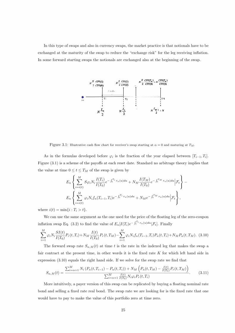
Figure 3.1: Illustrative cash flow chart for receiver’s swap starting at α = 0 and maturing at TM .

As in the formulas developed before ϕi is the fraction of the year elapsed between [Ti−1, Ti].

Figure (3.1) is a scheme of the payoffs at each reset date. Standard no arbitrage theory implies that

the value at time 0 ≤ t ≤ TM of the swap is given by

En

M∑

i=i(t)

SϕiNiI(Ti)I(T0)

e−R Ti

t rn(u)du + NMI(TM )I(T0)

e−R TM

t rn(u)du∣∣∣Ft

−

En

M∑

i=i(t)

ϕiNifn(Ti−1, Ti)e−R Ti

t rn(u)du + NMe−R TM

t rn(u)du∣∣∣Ft

,

where i(t) = mini : Ti > t.We can use the same argument as the one used for the price of the floating leg of the zero-coupon

inflation swap Eq. (3.2) to find the value of En[I(Ti)e−R Ti

t rn(u)du|Ft]. Finally

M∑

i=1

ϕiNiSI(t)I(T0)

Pr(t, Ti)+NMI(t)

I(T0)Pr(t, TM )−

M∑

i=1

ϕiNifn(Ti−1, Ti)Pn(t, Ti)+NMPn(t, TM ). (3.10)

The forward swap rate Sα,M (t) at time t is the rate in the indexed leg that makes the swap a

fair contract at the present time, in other words it is the fixed rate K for which left hand side in

expression (3.10) equals the right hand side. If we solve for the swap rate we find that

Sα,M (t) =

∑Mi=α+1 Ni (Pn(t, Ti−1)− Pn(t, Ti)) + NM

(Pn(t, TM )− I(t)

I(T0)Pr(t, TM )

)

∑Mi=α+1

I(t)I(T0)

NiϕiPr(t, Ti). (3.11)

More intuitively, a payer version of this swap can be replicated by buying a floating nominal rate

bond and selling a fixed rate real bond. The swap rate we are looking for is the fixed rate that one

would have to pay to make the value of this portfolio zero at time zero.

25

This formula is also model independent and was derived solely with the principles of no arbitrage.

It is worth to mention that for its calculation it involves no correlations or volatilities between the

nominal and real rates or inflation. In the next section we present the pricing formula for a European

swaption, where the volatilities and correlations play an important role in the pricing formula.

3.3 Pricing European swaption

A swaption is an option to enter a swap. An option on the right to pay the fixed rate in a swap

is called a payer’s swaption. An option on the right to pay the floating rate i.e. receive the fixed

rate, is called a receiver’s swaption. When there is only one exercise date (generally the beginning

of a forward starting swap or a reset date to break a swap), it is called a European swaption. To

obtain the payoff of a payer’s swaption, we assume that the underlying swap has a fixed strike rate

of K, and the maturity date is the same as the beginning of the forward starting swap Tα. If we

substitute in equation (3.10), we know that the option will be exercised if

MX

i=1

Niϕi

f(Tα, Ti−1, Ti)Pn(Tα, Ti)−K

I(Tα)

I(T0)Pr(Tα, Ti)

+ NM

Pn(Tα, TM )− I(Tα)

I(T0)Pr(Tα, TM )

> 0 (3.12)

If we use the positive-part operator and the annuity factor

C(t) =M∑

i=α+1

ϕiNiPr(t, Ti)I(t)

I(T0)(3.13)

then the payoff of a payer’s swaption is

V (Tα) = (Sα,M (Tα)−K)+C(Tα), (3.14)

where Sα,M (t) is the market swap rate at time t of a swap that starts at Tα and matures at TM .

Similarly, the pay-off of a receiver’s swaption is

(K − Sα,M (Tα)+C(Tα).

The value at time t of an European swaption maturing at Tα under the Qn is given by

V (t) = En

[V (Tα) exp

(−

∫ Tα

t

rn(s)ds

)∣∣∣Ft

], (3.15)

this involves the simulation of an integral which is rather cumbersome. There is an alternative

approach that simplifies the calculations. If we change from the risk neutral measure to the T -

forward measure, i.e. we use the nominal discount bond Pn(t, T ) with T ≥ Tα as numeraire instead

of the nominal market account; the price of the swaption is given by

V (t) = Pn(t, T )ETn

[(Sα,M (Tα)−K)+

Pn(Tα, T )C(Tα)

]. (3.16)

26

To calculate the last expectation it is necessary to find the dynamics of the factors under the

T -forward measure5. Using the change of numeraire technique developed by Brigo and Mercurio

(2001) we find the processes for the nominal rate, real rate and inflation index under the T -forward

measure

drn(t) = [θn − anrn(t)− σ2nBn(t, T )]dt + σndWT

n (t) (3.17)

drr(t) = [θr − arrr(t)− ρr,IσIσr − σrσnρn,rBn(t, T )]dt + σrdWTr (t) (3.18)

dI(t)I(t)

= [rn(t)− rr(t)− σIσnρn,IBn(t, T )]dt + σIdWTI , (3.19)

where Bn(t, T ) = 1an

(1− e−an(T−t)).

Equations (3.17)-(3.18) can be expressed as Ornstein-Ulhenbeck process and can be easily inte-

grated up to time t conditional on Fs, 0 ≤ s ≤ t

rn(t) = rn(s)e−an(t−s) +∫ t

s

e−an(t−u)(θn(u)− σ2

nBn(u, T ))du (3.20)

+σn

∫ t

s

e−an(t−u)dWTn (u)

rr(t) = rr(s)e−ar(t−s) +∫ t

s

e−ar(t−u) (θr(u)− ρr,IσIσr − σnσrρn,rBn(u, T )) du (3.21)

+σr

∫ t

s

e−ar(t−u)dWTr (u)

Therefore, rn(t) and rr(t) conditional on Fs are normally distributed with mean and variance given

respectively by

E[rn(t)|Fs] = rn(s)e−an(t−s) + ϑn(t)− e−an(t−s)ϑn(s) (3.22)

+σ2

n

2an

[e−an(t−s)Bn(s, T )−Bn(t, T )−Bn(s, t)

],

Var[rn(t)|Fs] =σ2

n

2an[1− e−2an(t−s)], (3.23)

where

ϑn(t) = f∗n(0, t) +σ2

n

2a2n

(1− e−ant)2.

E[rr(t)|Fs] = rr(s)e−ar(t−s) + ϑr(t)− e−ar(t−s)ϑr(s)−Br(s, t)ρr,IσIσr + (3.24)

+ρn,rσnσr

an + ar

[e−ar(t−s)αBn(s, T )−Bn(t, T )−Br(s, t)

],

Var[rr(t)|Fs] =σ2

r

2ar[1− e−2ar(t−s)]. (3.25)

where

ϑr(t) = f∗r (0, t) +σ2

r

2a2r

(1− e−art)2.

5Recall the dynamics of the real and nominal rates and inflation index under the nominal money market accountare given by formulas (2.38)-(2.40).

27

The logarithm of the inflation index is normally distributed with mean and variance given by

E[log I(t)|Fs] = log I(Ts)

rn(t)− rr(t)− ρn,IσIσnBn(t, T )− 12σ2

I

(t− s) (3.26)

Var[log I(t)|Fs] = σ2I . (3.27)

Once we have the correct distribution of our factors under the T -forward measure it is straight-

forward to price the European swaption at any time. If we are interested in the value at time zero

t = s = 0 of the swaption, we use the bond maturing at Tα as numeraire. The pricing formula (3.16)

reduces to

V0 = Pn(0, Tα)ETαn [V (Tα)], (3.28)

since Pn(0, Tα) is known at time zero and Pn(Tα, Tα) = 1.

28

Chapter 4

Estimation of parameters andValuation using quasi-Monte CarloSimulation

4.1 Mexican Inflation Linked market

We are going to use data from Mexico to implement the model presented in the previous chapter.

The government of Mexico started issuing inflation indexed debt already in the 1970’s. More recently,

on May 30 1996, the government introduced inflation-linked securities called Udibonos; these are

coupon indexed bonds that pay semi-annual coupons linked to the (UDI), an inflation-linked unit of

value defined in terms of the Mexican CPI. They were issued to help extend the maturity of public

debt, to lower the cost of funding and to increase the range of public financing instruments. Later

in the 1990’s, the Mexican government issued the so called Pics which are similar to Udibonos but

having maturities up to 25 years. Given the existence of these inflation-linked bonds, it is possible to

build a real term structure. Since our focus in the following is on pricing options on inflation-linked

swaps, we assume that both the nominal and real interest rate curves have already been constructed.

The derivatives market on the other hand is not developed, there are a few over-the-counter

operations but there are no quotes in the market for caps or swap volatilities neither in nominal

market nor inflation-linked market. Therefore, it is not possible to calibrate the model to existing

prices or volatilities in the market.

For the estimation of volatilities and correlations involved in the Jarrow and Yildrim model we

use historical data of bond prices and inflation index.

4.1.1 Estimating parameters for nominal and real markets

“History tends to repeat itself.” Some risk analyst believe in this and that is the reason why it is a

common practice to test the performance of portfolios in historical conditions and/or stress scenarios

to assess how much money the company can loose if it does. For pricing, the approach is to use the

29

market data to estimate the fair price implied in the markets assuming there is no arbitrage. Our

approach is based in historical data for the estimation of the volatility of the rates and inflation and

correlation between the three factors given that the main interest is for risk management purposes

and not for speculation.

We used daily data of the nominal and real term structure curves from 01-January-2001 to 08-

June-20051. We recall we considered a one-factor volatility function for the nominal and real rates

of the form

σk(t, T ) = σke−ak(T−t) , k = r, n (4.1)

where σi and ai for i = r, n are constants, which allowed us to recover the Extended Vasicek model

for short rates. If we use the dynamics of bond prices under the nominal market measure (2.36) and

(2.37) we can derive that the bond returns evolve according to the following normal distribution:

∆Pk(t, T )Pk(t, T )

− [µk]∆t ∼ N

0,

(∫ T

t

σi(t, s)ds

)2

∆t

. (4.2)

If we use daily observations (trading days) ∆t = 1252 , the expected return on the bond is small

relative to the standard deviation so it is possible to neglect it from the estimation procedure [15].

So the variance of the zero-coupon bond prices over the time interval [t, t + ∆] satisfies the equation

var

(∆Pk(t + ∆, T )

Pk(t, T )

)=

σ2k(e−ak(T−t)−1)2)∆t

a2r

(4.3)

The correlation between nominal and real rates is also crucial for option pricing, we can estimate it

with formula

ρr,n = Corr(∆rr(t), ∆rn(t)) (4.4)

If we use the observations of the real and nominal zero coupon prices generated from the term

structures we can compute the sample variance as an estimate of left side of last expression. We can

use the cross-sectional data from different maturities of the zero-coupon bonds and with non-linear

regression estimate the parameters.

The resulting estimates of these parameters are:

ar = 0.04933 σr = 0.01543an = 0.13690 σn = 0.02668

ρn,r = 0.17750

1Source Price Provider Company Valmer Inc.

30

4.1.2 Estimation of parameters of Inflation

Jarrow and Yildrim assume that the inflation index follows a lognormal distribution. We are going to

analyse the time series of inflation to test if the inflation has seasonality and to examine the possible

side effects of our simplification. For estimation we use the Mexican INPC or CPI inflation index.

This index is published by the Mexican Central Bank with a lag of 1 month. So the monthly data

points are linearly interpolated to obtain a daily index called UDI which has two weeks lag with

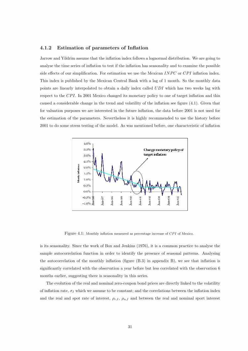
respect to the CPI. In 2001 Mexico changed its monetary policy to one of target inflation and this

caused a considerable change in the trend and volatility of the inflation see figure (4.1). Given that

for valuation purposes we are interested in the future inflation, the data before 2001 is not used for

the estimation of the parameters. Nevertheless it is highly recommended to use the history before

2001 to do some stress testing of the model. As was mentioned before, one characteristic of inflation

Figure 4.1: Monthly inflation measured as percentage increase of CPI of Mexico.

is its seasonality. Since the work of Box and Jenkins (1976), it is a common practice to analyse the

sample autocorrelation function in order to identify the presence of seasonal patterns. Analysing

the autocorrelation of the monthly inflation (figure (B.3) in appendix B), we see that inflation is

significantly correlated with the observation a year before but less correlated with the observation 6

months earlier, suggesting there is seasonality in this series.

The evolution of the real and nominal zero-coupon bond prices are directly linked to the volatility

of inflation rate, σI which we assume to be constant; and the correlations between the inflation index

and the real and spot rate of interest, ρr,I , ρn,I and between the real and nominal sport interest

31

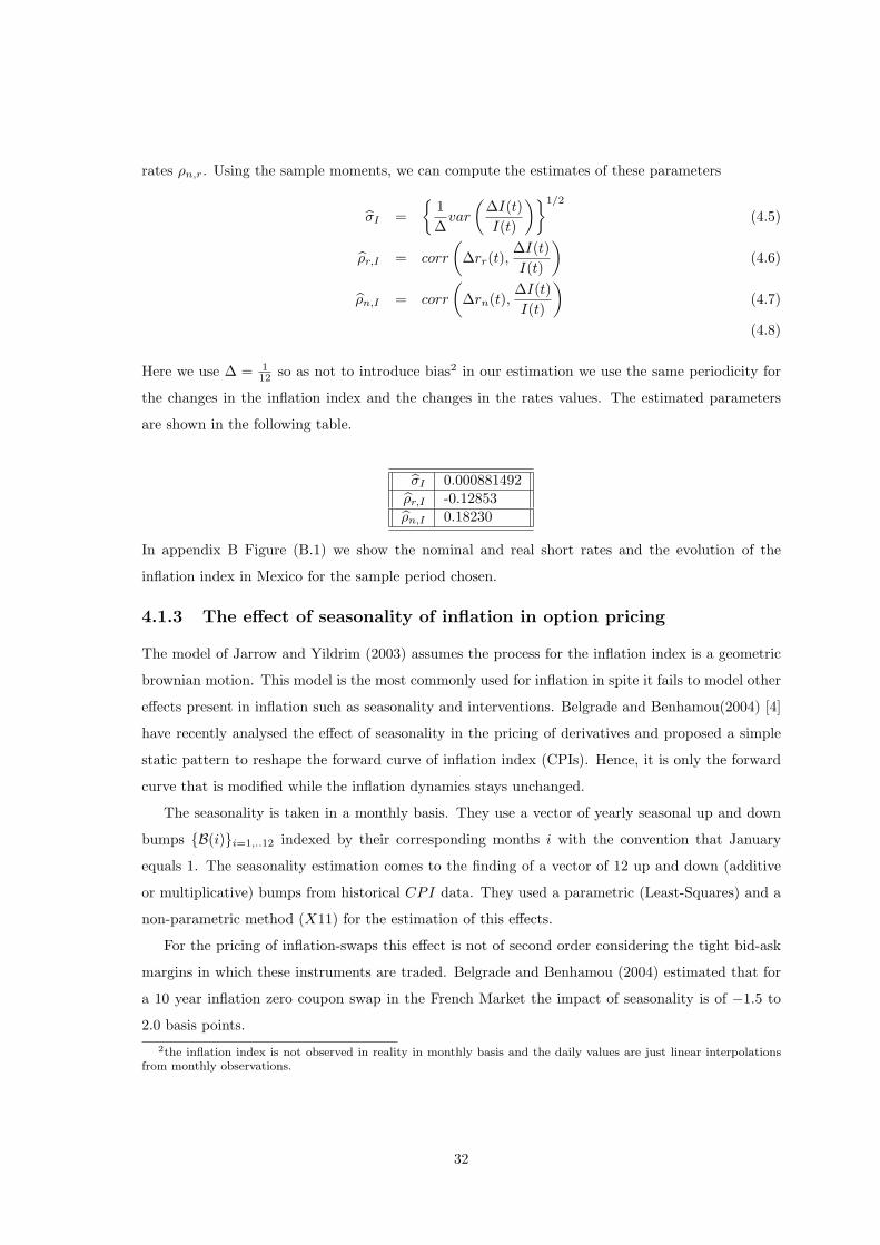
rates ρn,r. Using the sample moments, we can compute the estimates of these parameters

σI =

1∆

var

(∆I(t)I(t)

)1/2

(4.5)

ρr,I = corr

(∆rr(t),

∆I(t)I(t)

)(4.6)

ρn,I = corr

(∆rn(t),

∆I(t)I(t)

)(4.7)

(4.8)

Here we use ∆ = 112 so as not to introduce bias2 in our estimation we use the same periodicity for

the changes in the inflation index and the changes in the rates values. The estimated parameters

are shown in the following table.

σI 0.000881492ρr,I -0.12853ρn,I 0.18230

In appendix B Figure (B.1) we show the nominal and real short rates and the evolution of the

inflation index in Mexico for the sample period chosen.

4.1.3 The effect of seasonality of inflation in option pricing

The model of Jarrow and Yildrim (2003) assumes the process for the inflation index is a geometric

brownian motion. This model is the most commonly used for inflation in spite it fails to model other

effects present in inflation such as seasonality and interventions. Belgrade and Benhamou(2004) [4]

have recently analysed the effect of seasonality in the pricing of derivatives and proposed a simple

static pattern to reshape the forward curve of inflation index (CPIs). Hence, it is only the forward

curve that is modified while the inflation dynamics stays unchanged.

The seasonality is taken in a monthly basis. They use a vector of yearly seasonal up and down

bumps B(i)i=1,..12 indexed by their corresponding months i with the convention that January

equals 1. The seasonality estimation comes to the finding of a vector of 12 up and down (additive

or multiplicative) bumps from historical CPI data. They used a parametric (Least-Squares) and a

non-parametric method (X11) for the estimation of this effects.

For the pricing of inflation-swaps this effect is not of second order considering the tight bid-ask

margins in which these instruments are traded. Belgrade and Benhamou (2004) estimated that for

a 10 year inflation zero coupon swap in the French Market the impact of seasonality is of −1.5 to

2.0 basis points.2the inflation index is not observed in reality in monthly basis and the daily values are just linear interpolations

from monthly observations.

32

Nevertheless, if the focus of the model is to pricing of inflation-linked options, the seasonality

becomes of second order given that the main draw of the price is the volatility of the rates and

inflation and their correlations.

4.2 Quasi-Monte Carlo simulation

The pricing formula for the European swaption under the T -forward measure involves the calculation

of an expected value given in equation (3.28). The value of this expectation can be found by direct

integration, solving the partial differential equation that the relative price satisfies or by Monte Carlo

integration. In this case, we decided to use Monte Carlo simulation for several reasons: given that

the main goals of the implementation is to use the model for risk management and scenario analysis

it is the appropriate technique used for this purposes; consistency with the Longstaff and Schwartz

approach for pricing the Bermudan swaption; and if we decide to extend this model in the future to

a multifactor model such as Libor Market Model, it would have to use Monte Carlo for the pricing.

The basic Monte Carlo method is very simple, it essentially uses the law of large number to

evaluate the expectation. A central feature of Monte Carlo that the order of its error is O(N−1/2).

In order to add one decimal place of precision to the estimation of the price it requires 100 times as

much points, as a consequence to obtain high levels of accuracy one needs a large number of samples.

Monte Carlo simulation works because it tries to cover the unit interval in an even manner. However,

in the short term, the values may cluster around certain values which is why the simulation takes

a long time to converge. As Monte Carlo simulation is slow to converge, a lot of research has gone

into methods for increasing its speed of convergence, such as variance reduction techniques [16].

If instead we use a deterministic sequence of numbers that covers the interval, a low-discrepancy

sequence, the rate of convergence reduces to O(N−1−ε), ε > 0, where ε depends on the dimension

of the problem. Using low-discrepancy sequences to carry out Monte Carlo, is sometimes called

quasi-Monte Carlo3.

4.2.1 Quasi-Random Numbers: Faure Sequence

There are several types of low-discrepancy sequences: Halton sequences, Sobol’ sequences and Faure

sequences. In practice both Faure sequence and Sobol’ sequence are superior to the Halton sequence

[13]. Faure sequence has certain advantages for the valuation of high dimensional integrals [17].

We describe the algorithm presented in Boyle and Tan (96) for k-dimensions. Let p be the smallest

prime greater than max(k, 2), n the number of simulation. For each n, k Faure numbers are generated

3The term quasi-Monte Carlo can be misleading because the numbers are deterministically generated and do notpretend to be random.

33

recursively. Suppose that n =∑∞

j=0 a1jp

j , 0 ≤ a1j < p. Set

φ1p(n) =

∞∑

j=0

a1jp−j−1. (4.9)

For 1 ≤ s ≤ k, φsp is defined as

φsp(n) =

∞∑

j=0

asjp−j−1. (4.10)

where asj(n) are defined recursively. Suppose all as−1

j (n) are known, then

asj(n) =

∞∑

i≥j

iCjas−1j (n)mod p, (4.11)

where iCj = i!j!(i−j)! . Thus the next level of coefficients is obtained by multiplying by an upper

triangular matrix. The sequence of k-dimensional vectors φp(n)n=1,2,... is the k-dimensional Faure

sequence.

In order to generate the sequence, it is required to provide an initial point or “seed” to start the

recursions. This starting index must be greater than or equal to 1. Fox [9] recommends to use as

starting point p4 − 1 to improve uniformity.

The code used in our implementation is described in Fox (86) [9]. In Appendix B Table D we

show a table of the first 12 points generated for three dimensions in base 3 with initial point equal

to 1. In figure D.1 we show the points in plots onto two dimensions and in the cube, where we

can appreciate how they are evenly distributed to cover it. We can notice that the projections in

[1, 0)2 are identical when the distance between the factors is equal and the projection of Factor 3

and Factor 1 is equal but exchanging the axes. This phenomenon is caused by the cyclic properties

of the generator matrices, so the projections of the points in the ith and jth coordinates depends

only on the distance j − i, module the base p; further discussion of this result can be found in [10].

4.2.2 Generating Multivariate Normal Variables

To apply the Faure sequence to Monte Carlo simulation based on Normal random variables, we

map the point in the k-dimensional cube by applying the inverse normal function to the sequence

Φ−1(φn). For the inversion of the Normal distribution we use the algorithm given by Moro [16]4.

A multivariate normal distribution N(µ, Σ) is specified by its mean vector µ and covariance

matrix Σ. We know that if Z ∼ N(0, I) and X = µ + AZ, then X ∼ N(µ, AAᵀ). With the

method described above we can generate independent standard normal random variables obtained

with the inversion of the normal distribution on the Faure sequence. Thus, the problem of sampling

X reduces to finding the matrix A for which AAᵀ = Σ. A Cholesky factorization of Σ would give us

this matrix A. If Σ is positive definite, it has a Cholesky factorization and the matrix A is unique

up to changes in sign [10].4See the algorithm in Appendix D.1

34

We can simulate the nominal rate, the real rate and the logarithm of the inflation index as

multivariate normal distribution. Using the historical correlations and the mean and variance of the

three factors given by equations (3.22)-(3.25) and (3.26)-(3.27).

4.2.3 Analysis of Results

We are going to assume a flat term structure of real and nominal rates, using as reference the market

rates from 8 July 2005 in Mexico, the nominal spot rate equal to 12% and real spot rate equal to

4.5%. The inflation index used as reference is today’s index value assume equals IT0 = 1. All this

analysis (unless stated contrary) are based on a payer’s swaption that matures in one year. Its

underlying swap is a fixed real vs. floating nominal forward5 starting swap that starts also in one

year, has cash flow payments every six months and has a maturity of 5 years. We fixed the strike

of the swaption equal to the forward swap rate. In appendix C we present some graphs with the

results.

First we used 10,000 simulations (in theory to obtain close to four digits of precision). We

obtained the histograms and sample mean, standard deviation and correlation of each factor. We

verified that the sample values were very close to the theoretical or real values, see figure (C.11).

We also analysed the histogram of the payoff of the option at maturity as well as the underlying

swap rate at the maturity of the option. We find the results are consistent, all the swap rates were

below our strike would represent a payoff of zero in the option, see figure (C.12).

The next thing we analyse in an informal way is the the convergence of the method. It is not

possible to do a more formal analysis because we do not know the exact value of the price through

an analytical formula6. Graphically we see in (figure C.1) that the price of the option converges very

rapidly as we increase the number of simulations. In figure (C.2) we compare the price obtained

Monte Carlo with a variance reduction technique (antithetic sampling) for the same number of

simulations, we find the quasi-Monte Carlo is superior even with very few number of simulations.

Another interesting analysis is how the price changes as we increase or decrease the strike price.

This is because a hedger has to decide whether to hedge completely a position or use an option strike

out-of-the money and save on the cost of the option (figure C.3). The strike runs from K = .01 to

K = .04. As the strike is more in-the-money the option is more expensive because we would have

the right to enter a swap to pay a small fixed real rate in exchange of floating nominal rate, therefore

it is more likely to be exercised.

We also analysed what happens when we increase the maturity date of the option as we keep the

maturity date of the swap, i.e. we price European options for underlying swaps with less cash flows

each time (C.4). The underlying swap rate becomes very small and in some cases becomes negative

5It is described in section (3.2).6If we had the analytical solution for the price of the option we could plot the convergence and test if it is of order

O(1/n1 − ε) for ε > 0 depends on the number of dimensions [10].

35

as we evolve in the future. This is a consequence of the dynamics assumed for the inflation index. If

we recall the inflation index is modelled as a geometric brownian motion and its drift is derived from

the difference between the nominal and the real rates and a correction factor given by the change of

numeraire. When the difference between the nominal rate and the real rate is large (as is the case

for Mexico which is around 8%), the index grows exponentially and this sole effect causes that the

swap rate has to be negative in order make the present value of its cash flows equal to the value of

the floating nominal bond. This effect is not observed when the implied inflation (difference between

nominal and real rates) is not very big or when we are pricing a short dated swaption. So this is

a major drawback of this model, it is not suitable for pricing long dated instruments or with large

implied inflation.

One of the most important tests are how the price of the option changes as we change the

volatilities and correlations. We varied the volatility of each factor from .001 to .40 with increments

of .05 with constant correlations (historical). This analysis is presented graphically as surfaces of

the price of the option in figures (C.5)- (C.7) for each fixed value of the volatilities. We can conclude

that the price of the option is very sensitive to the volatility of the real rate, secondly to the volatility

of the inflation index and at last the volatility of the nominal rate. The volatility of the real rate has

the major effect because of the annuity term is involved in the pricing formula. As we mentioned

before, the level of the inflation index a determinant factor in the price of the option, and its volatility

has an effect in the simulated values of inflation. It is worth to mention that using historical data,

the volatility of the nominal rate is twice as big as the volatility of the real rates and almost 3

times bigger than the volatility of the inflation index. In periods of economic crisis the volatility of

inflation usually rises and this would have a major effect in the price of the option, more than the

effect of an increase in the volatility of the nominal rate.

We did a similar analysis to correlations, we changed the correlation between each pair of factors

from -.75 to .75 with increments of .25. In this case we had to be careful that the resulting covariance

matrix was still positive definite to be able to have a Cholesky factorization of it. When the resulting

covariance matrix was not positive definite, we assumed the price of the option was zero. The shapes

of the resulting surfaces are more complex than the analysis we presented for volatilities; see figures

(C.8)-(C.10). Graphically we can see that the shape of the surfaces is the same when the fix the

correlation between the nominal rate and inflation and the real rates and inflation. This means that

a change in their correlation would produce similar effects on the price of the option. On the other

hand, when we fix the correlation between the nominal and real rates, the surfaces have a different

pattern, which tends to have more stable behaviour. The price of the option reaches its maximum

when the correlation between nominal rates and the inflation is large and negative, and when there

is no correlation among the factors. This is a very interesting result as in periods of crisis, the

correlations may change sign or become apparently independent from one and another. The price

36

of the option on the other hand is small when we have positive correlation between real rates and

inflation, and when the correlation of the nominal rate and inflation index is either low or zero. In

this case, when the real rates and inflation index have positive correlation7, it means that if the

inflation increases, the real rate would also increase. Hence, the cash flow of the inflation indexed

leg will increase because of these two effects, the swap rate will decrease and it is less likely that the

the option will be exercised.

7Recall the historical correlation is negative.

37

Chapter 5

Bermudan Swaption

Bermudan swaptions are options to enter a swap not only in a single date, but at a sequence of

dates.

For pricing Bermudan swaptions with the Jarrow and Yildrim (2003) we are going to use Longstaff

Schwartz “Monte Carlo Regression” or “Least Squares Monte Carlo” (LSMC). This method is quite

general and has been used in practice to price interest rate Bermudan swaptions with LIBOR Forward

Models (see Brigo and Mercurio [6]).

5.1 Longstaff and Schwartz Approach

Longstaff and Schwartz (2001) developed a method to value American and Bermudan-style options

by simulation. This approach is readily applicable in path-dependent and multifactor situations

where traditional finite difference techniques or lattice methods cannot be used. At any exercise

time, the holder of the Bermudan-option optimally compares the payoff from immediate exercise

with the expected payoff from continuation, and then exercises if the immediate payoff is higher.

Therefore, the optimal exercise strategy is determined by the conditional expectation of the payoff

from continuing to keep the option alive. This method estimates the conditional expectation from

cross-sectional information in the simulation by using least squares. Specifically, the ex-post realised

payoffs from continuation are regressed on functions of the values of the state variables. The fitted

value from this regression provides a direct estimate of the conditional expectation function. By

estimating the conditional expectation function for each exercise date, it is possible to obtain a

complete specification of the optimal exercise along each path.

5.1.1 Valuation framework

The underlying LSM algorithm is based on the general derivative pricing paradigm of Black and

Scholes (1973) and Heath, Jarrow and Morton (1992), and others. We assume given a complete

probability space (Ω,F , P ) and finite time horizon [0, T ], the sample space Ω is the set of all possible

realisations of the stochastic economy between time 0 and T and has typical ω representing a sample

38

path, F is the sigma field of distinguishable events at time T , and P is a probability measure defined

on the elements of F . We define F = Ft; t ∈ [0, T ] to be the augmented filtration generated by

the price processes for the securities in the economy, and assume that FT = F . Consistent with the

no-arbitrage paradigm, we assume the existence of an equivalent measure Q for this economy.

We are interested in valuing Bermudan-style derivative securities with random cash flows oc-

curring during the period [0, T ]. We restrict our attention to the derivatives with payoffs that are

elements of the space of square-integrable or finite variable functions L2(Ω,F , Q). This condition is

justified if we assume the conditional expectation is an element of the L2 space of square-integrable

functions relative to some measure, since L2 is a Hilbert space, it has a countable orthonormal basis

and the conditional expectation can be represented as a linear function of the elements of the basis.

The value of an American-Bermudan option equals the maximized value of the discounted cash flows

from the option, where the maximum is taken over all stopping times with respect to the filtration F .

Let C(ω, s; t, T ) denote the path of the cash flows generated by the option, conditional on the option

not being exercised at or prior to time t and on the optionholder following the optimal stopping strat-

egy for all s, t < s ≤ T . The objective of the LSM algorithm is to provide a pathwise approximation

to the optimal stopping rule that maximises the value of the American-Bermudan option. In the

Bermudan case, the option can only be exercised at the L discrete times 0 < t1 ≤ t2 ≤ ... ≤ tL = T ,

and consider the optimal stopping policy at each exercise date. At the final expiration date of the

option, the investor exercises the option if it is in the money, or allows it to expire if it is out of the

money. At exercise time prior to the final expiration date, the optionholder must choose whether to

exercise immediately or to continue the life of the option and consider the exercise decision at the

next exercise time. The value of the option is maximised pathwise, and hence unconditionally, if the

investor exercises as soon as the immediate exercise value is greater than or equal to the value of

continuation. At time tl, the cash flow and value of immediate exercise is the same and it is known

to the investor; the cash flows from continuation are of course not known. No arbitrage valuation

theory implies that the option cannot be exercised until time tl and is estimated by the expectation

of the remaining discounted cash flows C(ω, s; tl, T ) with respect to the risk-neutral pricing measure

Q. The value from continuation at time tl can be expressed as

F (ω, tl) = EQ

L∑

j=l+1

exp(−

∫ tj

tl

r(ω, s)ds

)C(ω, tj ; tl, T )|Ftl

(5.1)

where r(ω, t) is the stochastic riskless (nominal or real) discount rate, and the expectation is taken

conditional on the information set Ftlat time tl. So the problem of optimal exercise reduces

to comparing the immediate exercise value with this conditional expectation, and then exercising

as soon as the immediate exercise value is positive and greater than or equal to the conditional

expectation.

39

The LSM approach uses least squares to approximate the conditional expectation function at

tL−1, tL−2, ..., t1. The algorithm works backwards since the path of cash flows C(ω, s; t, T ) generated

by the option is defined recursively; C(ω, s; tl, T ) can differ from C(ω, s; tl+1, T ) since it may be

optimal to stop at time tl+1, thereby changing all subsequent cash flows along a realized path ω.

Specifically at time tl+1, we assume that the unknown functional form of F (ω; tL−1) in Equation (5.1)

can be represented as a linear combination of a countable set of FtL−1 -measurable basis functions.

There are many possible choices of basis functions for the regression. When the value of the

asset underlying the option is a Markovian process only current values of the state variables are

necessary, when they are non-Markovian, both current and past realisations of the state vari-

ables can be included in the basis functions and the regressions. Longstaff and Schwartz sug-

gest as one possible choice of basis functions the set of (weighted) Laguerre polynomials Ln =

exp(−X/2) eX

n!dn

dXn (Xne−X). With this specification, F (ω, tL−1) can be represented as

F (ω, tL−1) =∞∑

j=0

ajLj(X), (5.2)

where the aj coefficients are constants.

To implement the LSM approach, first it is necessary to approximate F (ω, tL−1) using the first

L < ∞ basis functions, denoted as FL(ω, tL−1). Once this subject of basis functions has been

specified,FL(ω, tL−1) is estimated by projecting or regressing the discounted values of C(ω, s; tL−1, T )

onto the basis functions for the paths where the options is in the money at time tL−1. Only in the

money paths are used in the estimation since the exercise decision is only relevant when the option

is in the money. By focusing on in-the-money paths, the region where the conditional expectation

has to be estimated is limited consequently less basis functions are needed to obtain an accurate

approximation to the conditional expectation function. Since the values of the basis functions are

independently and identically distributed across paths, the fitted value of the regression FL(ω, tL−1)

converges in mean square and in probability to FL(ω, tL−1) as the number of in-the-money paths in

the simulation goes to infinity.

Once the conditional expectation function at time tL−1 is estimated, it is possible to determine

whether early exercise at time tL−1 is optimal for an in-the-money path ω by comparing the imme-

diate exercise value with FL(ω, tL−1) and repeating for each in-the-money path. Once the exercise

decision is identified, the option cash flow paths C(ω, s; tL−2, T ) can be approximated. The recursion

proceeds by rolling back to time tL−2 and repeating the procedure until the exercise decision at each

exercise time along each path have been determined.

The Bermudan option is the valued by starting at time zero, moving forward along each path until

the first stopping time occurs, discounting the resulting cash flow from exercise back to time zero,

and then taking the average over all paths ω. When there are two state variables X and Y , the set of

basis functions should include terms in X and Y , as well as cross-products of these terms. Similarly

40

for higher-dimensional problems. Longstaff and Schwartz through some numerical examples suggest

that the number of basis functions necessary to approximate the conditional expectation grow slowly

than exponentially.

Theoretically, when the American option is continuously exercisable, for any finite choice of M, L

and vector θ in RM×(L−1) representing the coefficients for the M basis functions at each of the L−1

early exercise dates, let LSM(ω; M,L) denote the discounted cash flow resulting from following the

LSM rule of exercising when the immediate exercise value is positive and greater than or equal to

FL(ωi, tL−1) as defined by θ. Then the following inequality holds almost surely,

V (X) ≥ limN→∞

1N

N∑

i=1

LSM(ωi,M,L). (5.3)

The LSM algorithm results in a stopping rule for an American-style option. The value is based on

the stopping rule that maximises the value of the option; all the other stopping rules, including the

stopping rule implied by the LSM algorithm, result in values less than or equal to that implied by

the optimal stopping rule. This criterion then provides guide in determining the number of basis

functions needed to obtain an accurate approximation; simply increase the number of basis functions

M until the value implied by the LSM algorithm no longer increases. But by its nature providing a

general convergence result for the LSM algorithm is difficult since it is needed to consider limits as

the number of discretisation points L, the number of basis functions M , and the number of paths

N go to infinity.

5.1.2 Least-Square Monte Carlo for Bermudan Swaption

Originally Longstaff and Schwartz tested their method considering a version of a string model for

swaptions. In the Bermudan swaption considered here, the underlying swap starts at the first exercise

date of the option. The swaption holder has the right to exercise the option at some fixed dates and

enter the swap whose life span decreases as time moves forward. This option could be used to break

the underlying swap in fixed reset dates.

As Longstaff and Schwartz suggested in their paper, we use a the quasi-Monte-Carlo technique

(Faure sequence) described in the last chapter in conjunction with LSMC to improve the computa-

tional speed and efficiency. Faure sequences are still suitable for this problem since we are dealing

with a small number of dimensions (in our case a maximum of 12 dimensions=3 Factors x 4 time

steps), this problem is similar to the swaption priced by Joy et al.[17]. For a larger number of

exercise dates we support the recommendation of Glasserman [10] of using Sobol’ sequences or the

principal component algorithm developed by Akesson and Lehoczky [1].

The underlying swap we used is the same used in our European case. It matures in five years,

resets every six months, and exercise can occur once a year, one year included and five years excluded.

41

There are therefore five exercise dates and at each exercise date the underlying swap has two less

coupons than in the previous exercise date.

For Bermudan case, it is necessary to simulate the factors at discrete time steps (each exercise

date). A convenient choice of numeraire in this case is the nominal bond that matures at the last

exercise date of the Bermudan swaption (say TM−2). The distribution of the parameters at each time

step is derived from equations (3.22)-(3.27) using proper values for s = 0, Ti, Ti+1, TM−1 as exercise

dates and previous values of the factors rn(0), rr(0), I(0), ..., rn(TM − 2), rr(TM − 2), I(TM − 2).Once we run the algorithm and we estimated the optimal stopping time, we can estimate the price

of the option

V0 = Pn(0, TM−2) supi

ETM−2

[VTi

Pn(Ti, TM−2)

], i = 1, ..., TM−2. (5.4)

This is a straightforward calculation given that the Hull-White model has an analytical expression for

Pn(t, T ). For the estimation of the conditional expectation we used as basis functions a constant,the

first two powers of the swap rate, the factors and the cross product of the factors, resulting in 4 for

one factor model, 6 for two factor model and 9 for the three factor model.

Using the values of the Mexican Market, we found that the optimal stopping time was always in

the first exercise date or never to exercise the option. This is a result of the model for the inflation

index, it is growing un proportionally and the future swap rates result very small or even negative,

therefore the option is not exercised (figure C.13). When we changed the current nominal rate and

real rate to decrease the gap between them, we found there were some paths with different stopping

times than the first exercise date.

We analysed the effect of a reduction in the number of factors in the price of the Bermudan

swaption. For this exercise we changed the term structure of rates to be 6% the nominal rate and

4.5% the real rate in order to obtain some stopping times different from the first exercise date. It

is important to consider a reduction in the number of parameters because if we were interested in

increasing the number of exercise dates, the problem would soon become of very high dimensionality.

The inflation index has a small historical volatility compared to the volatility of the other two

factors, therefore when we assume its behaviour is deterministic. We can observe in figure (C.15)

that the price does not get significantly affected with the reduction to two factors, especially when

we increase the number of simulations. On the other hand when we assume both the real rate and

the inflation index have deterministic behaviour the price of the option drops considerably (figure

C.14). Therefore, we do not suggest to use a one factor model for the pricing of this option.

42

Chapter 6

Conclusion

To price inflation indexed derivatives one needs to know the theory behind interest rate modelling

and foreign-currency modelling, combined with some economic intuition. To produce a sensible

model one has to consider the dynamics of the nominal and real markets and the inflation index.

The three factor HJM model (foreign-currency analogy) allows one to treat the real rate the rates in

a foreign economy, and the inflation index (CPI) as the spot exchange rate in a framework consistent

with no arbitrage. We assumed a volatility function as in an Extended Vasicek model for the nominal

and real rates, as in Jarrow and Yildrim (2003). We developed the pricing formulas for an European

Swaption and implemented the pricing model using quasi-Monte Carlo simulation based on historical

data for the estimation of the parameters of the model. Finally we implemented the Longstaff and

Schwartz algorithm for the pricing of a Bermudan swaption. All the algorithms were programmed

for Matlab.

We confirmed that the Gaussian affine model used (Extended Vasicek) is very tractable and has

a number of characteristics that enables us to have good numerical valuation procedures, although

the estimation of its parameters is not straightforward. For the estimation of the parameters we used

historical data of the past five years of the Mexican economy. We used daily data for the estimation

of the volatilities of the nominal and real rates, and a non-linear least squares algorithm for the

estimation of the mean reversion of the nominal and real spot rates. The volatility of the inflation

index and the correlation with the nominal rate and real rate was using monthly observations. This

models permit rates to become negative with non-zero probability, but as is discusses in [13] we

found that when this model is fitted to “ordinary” term structures this probability is very low1.

Furthermore, for markets like Mexican where there is no active trading of options there is no need

to calibrate the model with market quotes and one factor models for the nominal and real interest

rates are adequate. We suggest as a natural extension for this model to incorporate the multifactor

nature of the term structure of the nominal and real rates as in the Libor Market Model.1Although this might not be the case in markets with low levels interest rates.

43

We found that the geometric brownian motion model for the inflation index is not realistic because

historically there are other effects present in the series of the inflation index such as seasonality and

interventions; however, assuming it is a simple geometric brownian motion provides a good level of

tractability to the model. More specifically for option pricing there is one major shortcoming of

this model. When the drift (estimated as the difference between the nominal rates and real rates) is

large, the model is inappropriate for pricing long dated options (probably not more than 2 years),

even with a small implied inflation (around 2%) the model would not be applicable for options dated

more than 5 years. It would cause a significant underpricing of the option (in the payer’s version)

and an overpricing for the receiver’s version. The improvement in the dynamics of the inflation

index should be one of the main areas for future work. The new models should incorporate jump

diffusion processes (for interventions), seasonality (deterministic or stochastic), mean reversion for

the inflation and/or include not only short term but long term interest rates on its dynamics to

improve the modelling of its drift.

The parameters of the model that need to be monitored closely are the volatilities and correlations

between the factors. The price or value of the option is very sensitive to these parameters, specially to

the volatility of real rates and inflation, and the correlation between the nominal rates and inflation.

In periods of crisis in the markets this parameters tend to change rapidly and it has been often the

case that the correlations change sign or the factors behave independently. This situation should

be considered very closely in markets where there the parameters have to be estimated historically.

It might take a few observations before the estimated parameters take the change in volatilities or

correlations, so it is important to have alternative methods to identify rapidly these changes and use

them for pricing the option.

Monte Carlo models and specifically quasi-Monte carlo techniques are very convenient for risk

management, scenario analysis and valuation of large portfolios as mentioned by Joy et at.[17]. We

confirmed that quasi-Monte Carlo methods produce substantially more precise values than ordinary

Monte Carlo for the pricing of the European Swaption. For calculations that need to be repeated

often with only minor change in parameters (such as sensitivity of price to some parameters or

price an option everyday) quasi-Monte Carlo is very time effective. However there is an important

feature of quasi-Monte Carlo methods that has to be considered, its dependence on the dimension

of the problem. In our examples we treated low dimensional problems (3-12 dimensions) with

Faure sequences, but it we advice to analyse the benefits of using other low discrepancy series such

as Sobol’ if one desires to increase significantly the dimensionality of the problem (increasing the

number of factors or time steps). Furthermore, we suggest to derive the semi-analytical formulas

for the European swaption or implement finite difference methods and compare the results obtained

with the three methods.

44

For the pricing of the Bermudan swaption the Longstaff and Schwartz approach is in principle

simple to implement. One has to choose a convenient numeraire, generate the paths for the under-

lying of the option, and choose the basis functions for the estimate of the conditional expectation

(using the least-squares). In all the models we used as basis functions one constant, the first three

powers of the underlying swap, the factors and the crossed products of the factors. As it is men-

tioned in [18] we included more basis functions but we did not find an increase in the fitness of the

model. Finally we find the optimal stopping time for each path and average the discounted cash

flows. Using the market rates for Mexico, the optimal stopping time was in the first exercise date

or not exercise the option at any time. This is a consequence of the effect of the exponential growth

of the inflation index in time. We consider the price of the Bermudan option with out algorithm

should be taken as a lower bound to the price of the Bermudan swaption when dealing with long

dated swaptions or large implied inflation.

For the pricing of the Bermudan swaption with multiple exercise dates, one should consider the

benefits of decreasing the number of factors in terms of the desired accuracy of the results with the

tractability of the model. We found that the difference from using a one factor model to a three

factor model can be considerable (15% with our data) and this might increase if the volatility of

the factors that we are eliminating is bigger than in our example. A more detailed analysis of the

sensitivity of the price of the Bermudan option as we change the volatilities and correlations should

be considered before going from the three factor model to some simplification of it.

45

Appendix A

Glossary

Affine : f is an affine function of X if f(X) = a + bX.

Arbitrage :Arbitrage is guaranteed way of making money without risk.

BTP :Italian Buoni Poliennali del Tesoro. The inflation-indexed BTP is often referred to as a

BTPEi, indexed to Euro-HICP excluding tobacco.

CIBs : Australian Capital Indexed Bond.

CPU-I :non-seasonally adjusted US City Average All Items Consumer Price Index for All Urban

Consumers.

Duration : is defined as a weighted average of the coupon dates of a bond where the discounted

values of the coupon payments are used as weights,and it will provide the “mean time to

coupon payment”. It is a measure of the sensitivity of the bond price with respect to changes

in the yield. For a bond with coupons ci with price at t = 0 equal to P , yield to maturity y

and coupon payments at Ti, the duration D is defined as:

D =∑n

i=1 Ticie−yTi

P

Euro-HICP : Euro-zone Harmonised Index of Consumer Prices.

Filtration : A set Ft0≤t≤Tmax of σ-algebras such that Ft1 ⊆ Ft2 for t1 ≤ t2, representing the

increase in information available by observing a stochastic system through time.

Gilt :UK government bonds.

In-the-money : Term commonly used in finance to say that the price of the underlying of an

option is in the region where it would be exercised giving a positive value for the optionholder.

Hilbert space :A Hilbert space is a vector space H with an inner product < f, g > such that the

norm defined by |f | =√

( < f, f >) turns H into a complete metric space. If the metric

defined by the norm is not complete, then H is instead known as an inner product space.

46

INPC :Indice Nacional de Precios al Consumidor, or Mexican CPI Index. This index is published

by the Central bank every two weeks with a lag of 1 month when the inflation actually occurred.

Fisher Equation :Formulated by Alan Fisher in the inter-war period before the start of the in-

flation indexed bond markets. It states that a nominal bond yield is made up of three com-

ponents: inflationary expectations, a required real yield that investors require over and above

those expectations and a “premium” that reflects the assumption that investors want addi-

tional compensation for accepting additional inflationary risks when holding nominal bonds.

Martingale :A stochastic process is a martingale if Et[ST ] = St, for all times t ≤ T . That is the

expected value in the future conditioned on what is known now is always identical to today’s

value.

OATi :French inflation indexed bonds or Obligations assimilables du Tresor. Its indexation is based

on the final non seasonally-adjusted French CPI ex-tobacco index.

RRB :Canadian Real Return Bond. They are coupon indexed bonds that pay semi-annual coupons,

the indexation is based on cumulative movements in the CPI.

SBIL : Greek inflation indexed bonds or State Bonds Index Linked.

TIPS : US Treasury Inflation-Protected Securities, are securities whose principal is tied to the

inflation rate. They bear a stated interest rate, and the owner receives semi-annual interest

payments. They are issued in terms of 5, 10, and 20 years.

Wiener process : A stochastic process W that meets the following conditions

1. W (0) = 0

2. The process W has independent increments, i.e. if r < s ≤ t < u then W (u)−W (t) and

W (s)−W (r) are independent stochastic variables.

3. For s < t the stochastic variable W(t)-W(s) has the Gaussian distribution N(0,√

t− s)

4. W has continuous trajectories

5. Stop rule

47

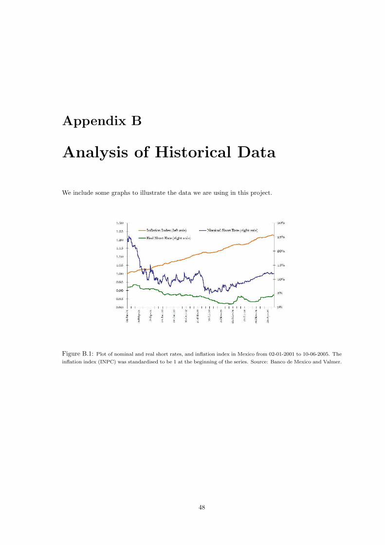
Appendix B

Analysis of Historical Data

We include some graphs to illustrate the data we are using in this project.

Figure B.1: Plot of nominal and real short rates, and inflation index in Mexico from 02-01-2001 to 10-06-2005. The

inflation index (INPC) was standardised to be 1 at the beginning of the series. Source: Banco de Mexico and Valmer.

48

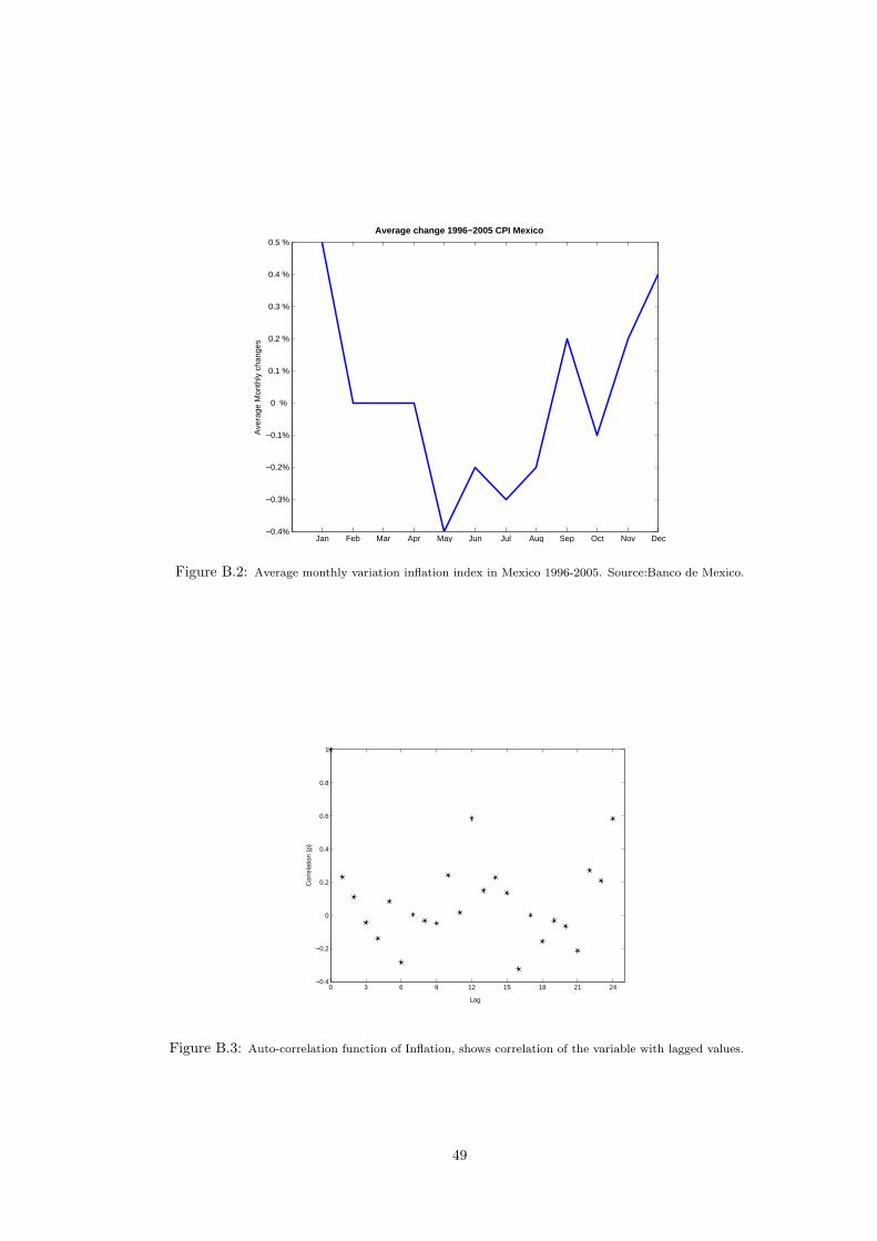
Jan Feb Mar Apr May Jun Jul Aug Sep Oct Nov Dec−0.4%

−0.3%

−0.2%

−0.1%

0 %

0.1 %

0.2 %

0.3 %

0.4 %

0.5 %

Ave

rage

Mon

thly

cha

nges

Average change 1996−2005 CPI Mexico

Figure B.2: Average monthly variation inflation index in Mexico 1996-2005. Source:Banco de Mexico.

0 3 6 9 12 15 18 21 24−0.4

−0.2

0

0.2

0.4

0.6

0.8

1

Lag

Cor

rela

tion

(ρ)

Figure B.3: Auto-correlation function of Inflation, shows correlation of the variable with lagged values.

49

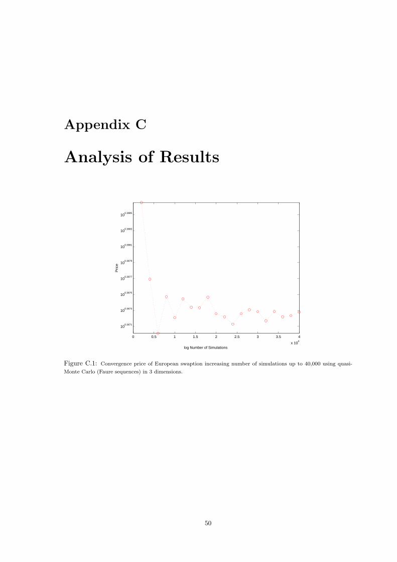
Appendix C

Analysis of Results

0 0.5 1 1.5 2 2.5 3 3.5 4

x 104

100.3871

100.3873

100.3875

100.3877

100.3879

100.3881

100.3883

100.3885

Pric

e

log Number of Simulations

Figure C.1: Convergence price of European swaption increasing number of simulations up to 40,000 using quasi-

Monte Carlo (Faure sequences) in 3 dimensions.

50

1000 2000 3000 4000 5000 6000 7000 8000 9000 100002.41

2.42

2.43

2.44

2.45

2.46

2.47

2.48

2.49

2.5

Numer of simulations

Pric

e

Quasi Monte CarloMonte Carlo

Figure C.2: Convergence price of European swaption increasing number of simulations. Monte Carlo with variance

reduction technique (antithetic sampling) and quasi-Monte Carlo (Faure sequences)

0 0.02 0.04 0.06 0.08 0.1 0.12 0.14 0.16 0.18 0.20

1

2

3

4

5

6

7

8

Strike Swap Rate

Pric

e

Figure C.3: Price of swaption increasing the strike K.

51

1 1.5 2 2.5 3 3.5 4 4.50

0.5

1

1.5

2

2.5

Time to maturity (Fixed maturity date)

Pric

e

Figure C.4: Price of swaption increasing the maturity of swaption, fixed maturity date of underlying swap.

0 .18 .400 .18

.400

10

20

30 σn =0.001

0 .18 .400 .18

.400

10

20

30 σn =0.045444

0 .18 .400 .18

.400

10

20

30 σn =0.089889

Pric

e

0 .18 .400 .18

.400

10

20

30σ

n =0.13433

0 .18 .400 .18

.400

10

20

30σ

n =0.17878

0 .18 .400 .18

.400

10

20

30σ

n =0.22322

Pric

e

0 .18 .400 .18

.400

10

20

30 σn =0.26767

Pric

e

0 .18 .400 .18

.4010

20

30 σn =0.31211

0 .18 .400 .18

.4010

20

30

40σ

n =0.35656

σI

σr

Figure C.5: Surface of price varying the volatility of the 3-Factors. Each surface corresponds to different value of

volatility of the nominal rate, x-axis is volatility of the inflation index,y-axis volatility of the real rate.

52

0 .18 .400.18

.400

10

20

30σ

I =0.001

0 .18 .400 .18

.400

10

20

30σ

I =0.045444

0 .18 .400 .18

.400

10

20

30σ

I =0.089889

0 .18 .4005

100

10

20

30σ

I =0.13433

0 .18 .400 .18

.400

10

20

30σ

I =0.17878

0 .18 .400 .18

.400

10

20

30σ

I =0.22322

0 .18 .400 .18

.400

10

20

30σ

I =0.26767

Pric

e

0 .18 .400 .18

.400

10

20

30σ

I =0.31211

0 .18 .400 .18

.4010

20

30

40σ

I =0.35656

σn

σr

Figure C.6: Surface of price varying the volatility of the 3-Factors. Each surface corresponds to different value of

volatility of inflation, x-axis is volatility of the real rate,y-axis volatility of the nominal rate.

0 .18 .400 .18

.400

10

20 σr =0.001

0 .18 .400 .18

.405

10

15

20 σr =0.045444

0 .18 .400 .18

.4010

15

20 σr =0.089889

0 .18 .400 .18

.4010

15

20

25σ

r =0.13433

0 .18 .400 .18

.4015

20

25 σr =0.17878

0 .18 .400 .18

.4015

20

25

30σ

r =0.22322

0 .18 .400 .18

.4020

25

30σ

r =0.26767

Pric

e

0 .18 .400 .18

.4024

26

28

30σ

r =0.31211

0 .18 .400 .18

.4025

30

35σ

r =0.35656

σn

σI

Figure C.7: Surface of price varying the volatility of the 3-Factors. Each surface corresponds to different value of

volatility of the real rate, x-axis is volatility of the nominal rate,y-axis volatility of the inflation index.

53

−.750

.75−.75

0.750

2

4 ρn,r

=−0.75

Pric

e−.75

0.75

−.75

0.750

2

4ρ

n,r =−0.5

Pric

e

−.750

.75−.75

0.750

2

4 ρn,r

=−0.25

Pric

e

−.750

.75

−.75

0.750

2

4ρ

n,r =0

Pric

e

−.750

.75

−.75

0.750

2

4ρ

n,r =0.25

Pric

e

−.750

.75

−.75

0.750

2

4 ρn,r

=0.5

Pric

e

−.75

0

.75 −.750

.75

0

2

4

ρn,r

=0.75

Pric

e

ρn,I

ρ

r,I

Figure C.8: Surface of price varying the correlation of the 3-Factors. Each surface corresponds to different value of

correlation between the nominal and real rates.

−.750

0.75

−.75

0 0.75

0

2

4ρ

n,I =−0.75

−.750

0.75

−.75

0 0.75

0

2

4ρ

n,I =−0.5

−.750

0.75

−.75

0 0.75

0

2

4 ρn,I

=−0.25

−.750

0.75

−.75

0 0.75

0

2

4ρ

n,I =0

−.750

0.75

−.75

0 0.75

0

2

4ρ

n,I =0.25

−.75

0

0.75 −.750

0.75

0

2

4

ρn,I

=0.5

−.75

0 0.75 −.75

0 0.75

0

2

4ρ

n,I =0.75

Pric

e

ρn,r

ρr,I

Figure C.9: Surface of price varying the correlation of the 3-Factors. Each surface corresponds to different value of

correlation between the nominal and inflation index.

54

−.750

.75

−.75

0.750

2

4 ρr,I

=−0.75

−.750

.75

−.75

0.750

2

4 ρr,I

=−0.5

−.750

.75

−.75

0.750

2

4ρ

r,I =−0.25

−.75 0 .75−.750

.750

1

2

3ρ

r,I =0

−.750

.75

−.75

0.750

2

4 ρr,I

=0.25

−.750

.75

−.75

0.750

2

4ρ

r,I =0.5

−.75

0.75

05

10

0

2

4 ρr,I

=0.75

Pric

e

ρn,I

ρn,r

Figure C.10: Surface of price varying the correlation of the 3-Factors. Each surface corresponds to different value

of correlation between the real rate and the inflation index.

0.1 0.15 0.2 0.25 0.3 0.350

0.05

0.1

0.15

0.2

0.25

0.3

0.35Nominal Spot rate

Min =0.1291 Max =0.3166 Mean =0.2246 Stdev=0.02573

freq

uenc

y in

per

cent

age

0 0.05 0.1 0.15 0.20

0.05

0.1

0.15

0.2

0.25

0.3

0.35Real Spot rate

Min =0.02563Max =0.1373 Mean =0.08401Stdev=0.01502

freq

uenc

y in

per

cent

age

1.08 1.0850

0.05

0.1

0.15

0.2

0.25

0.3

0.35Inflation index

Min =1.077 Max =1.083 Mean =1.08 Stdev=0.0009225

freq

uenc

y in

per

cent

age

Correlations Theo Sample Nominal and real 0.17 0.14 Nominal and inflation 0.18 0.176Real and inflation 0.13 −0.164

Theoretical ValuesFactor Mean Std.Dev Nominal Rate 0.22465 0.024954Real Rate 0.084012 0.015057Inflation index 1.08 0.00088149

Figure C.11: Histogram of nominal short rate, real short rate and inflation index at maturity of option (1y), strike

3%, maturity of swap 5y.

55

−0.05 0 0.05 0.1 0.150

0.05

0.1

0.15

0.2

0.25

0.3

0.35

Min =−0.01992Max =0.09103 Mean =0.03247 Stdev=0.01481

Swap Rate at maturity

−5 0 5 10 15 200

0.1

0.2

0.3

0.4

0.5

0.6

0.7Payoff at maturity

Min =0 Max =20.98Mean =2.75 Stdev=3.577

Figure C.12: Histogram of simulated payoff of the option and swap rate at the maturity of the option. Maturity of

option (1y), strike 3%, maturity of swap 5y.

Figure C.13: Estimated paths of the swap rate used for the pricing of the Bermudan Swaption using 3 factors and

market data.

56

2000 4000 6000 8000 10000 12000 14000

13.3045

13.305

13.3055

13.306

13.3065

13.307

13.3075

Number of simulations

Pric

e

Figure C.14: Convergence of price of Bermudan swaption increasing the number of simulations in one factor model

(nominal rate). The swaption has 5 annual exercise dates and strike 3%.

0 5000 10000 1500015.22

15.23

15.24

15.25

15.26

15.27

15.28

15.29

15.3

15.31

15.32

Number of Simulations

Pric

e

Figure C.15: Convergence of price of Bermudan swaption increasing the number of simulations in two factor model

(nominal and real rates) and three factor model (nominal rate,real rate and inflation index).

57

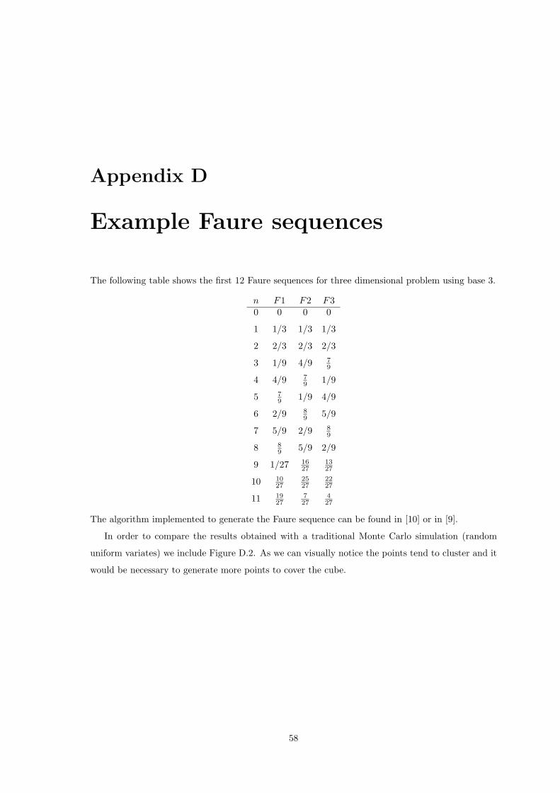
Appendix D

Example Faure sequences

The following table shows the first 12 Faure sequences for three dimensional problem using base 3.

n F1 F2 F30 0 0 0

1 1/3 1/3 1/3

2 2/3 2/3 2/3

3 1/9 4/9 79

4 4/9 79 1/9

5 79 1/9 4/9

6 2/9 89 5/9

7 5/9 2/9 89

8 89 5/9 2/9

9 1/27 1627

1327

10 1027

2527

2227

11 1927

727

427

The algorithm implemented to generate the Faure sequence can be found in [10] or in [9].

In order to compare the results obtained with a traditional Monte Carlo simulation (random

uniform variates) we include Figure D.2. As we can visually notice the points tend to cluster and it

would be necessary to generate more points to cover the cube.

58

0 0.2 0.4 0.6 0.8 10

0.2

0.4

0.6

0.8

1

Factor 1

Fac

tor

2

0 0.2 0.4 0.6 0.8 10

0.2

0.4

0.6

0.8

1

Factor 1

Fac

tor

3

0 0.2 0.4 0.6 0.8 10

0.2

0.4

0.6

0.8

1

Factor 2

Fac

tor

3

0

0.5

1

0

0.5

10

0.5

1

Factor 1Factor 2

Fac

tor

3

Figure D.1: Projections of 81 Faure points in 3 dimensions using base 3. The the figures show coordinates 1 and 2,

1 and 3, 2 and 3. Last 3-d scatter plot of points in the unit cube.

0 0.2 0.4 0.6 0.8 10

0.2

0.4

0.6

0.8

1

Factor 1

Fac

tor

2

0 0.2 0.4 0.6 0.8 10

0.2

0.4

0.6

0.8

1

Factor 1

Fac

tor

3

0 0.2 0.4 0.6 0.8 10

0.2

0.4

0.6

0.8

1

Factor 2

Fac

tor

3

0

0.5

1

0

0.5

10

0.5

1

Factor 1Factor 2

Fac

tor

3

Figure D.2: Projections of 81 random uniform points in 3 dimensions. The figures show coordinates 1 and 2, 1 and

3, 2 and 3. Last 3-d scatter plot of points in the unit cube.

59

D.1 The inverse cumulative normal function

The following is the code for Matlab of the algorithm proposed by Moro shown in [16] to evaluate

the inverse cumulative normal function for x ∈ (0, 1).

function w=inv_norm(x)

%This is B.Moro’s algorithm for inversion of the normal distribution

% x vector defined between 0 and 1

a(1)=2.50662823884; a(2)=-18.61500062529; a(3)=41.39119773534;

a(4)=-25.44106049637; b(1)=-8.47351093090; b(2)=23.08336743743;

b(3)=-21.06224101826; b(4)=3.13082909833;

c(1)=0.3374754822726147; c(2)=0.9761690190917186;

c(3)=0.1607979714918209; c(4)=0.0276438810333863;

c(5)=0.0038405729373609; c(6)=0.0003951896511919;

c(7)=.0000321767881768; c(8)=0.0000002888167364;

c(9)=0.0000003960315187;

for i=1:length(x)

y=x(i)-0.5;

if(abs(y)<0.42)

num=y.^2*[0:3]*a’;

den=y.^2*[1:4]*b’+1;

w(i)=y*num/den;

else

if y<0

r=x(i);

else

if (x(i)==1)

r=1^(-10);

else

r=1-x(i);

end

end

s=log(-log(r));

t=s.^[0:8]*c’;

if x(i)>.5

w(i)=t;

else

w(i)=-t;

end

end

end

60

Bibliography

[1] F. Akesson and J. Lehoczky. Path generation for quasi-monte carlo simulation for mortgage-

backed securities. Management Science, 46(9):1171–1187, Sep. 2000.

[2] Capital Research Barclays. Global inflation linked products: A user’s guide. Technical report,

January 2004.

[3] N. Belgrade, E. Benhamou, and E. Koehler. A market model for inflation. Preprint, CDC Ixis

Capital Markets, 2004.

[4] N. Belgrade and Benhamou E. Impact of seasonality in inflation derivatives pricing. CDC IXIS,

August 2004.

[5] T. Bjork. Arbitrage Theory in Continuous Time. Oxford University Press, 2nd edition, 2004.

[6] D. Brigo and F. Mercurio. Interest Rate Models Theory and Practice. Springer, 2001.

[7] M. Deacon and Derry A. Deriving estimates of inflation expectations from the prices of uk

government bonds. Bank of England, Working paper no. 23, July 1994.

[8] M. Deacon, A. Derry, and Mirfenderseki D. Inflation-indexed securities. Wiley Finance, 2nd.

ed. edition, 2004.

[9] P. Fox. Algorithm 647:implementation and relative efficiency of quasiramdom sequence gener-

ators. ACM Transactions on Mathematical Software, 12(4):362–376, December 1986.

[10] P. Glasserman. Monte Carlo Methods in Financial Engineering. Springer-Verlag, 2003.

[11] R. Hafer and Hein S. Forecasting inflation using interest rate and time series models:some

international evidence. The Journal of Business, 63(1):1–17, Jan. 1990.

[12] J. Hull and A. White. Pricing interest rate derivative securities. The Review of Financial

Studies, 3(4):573–592, 1990.

[13] J. James and Webber N. Interest Rate Modelling. Wiley and Sons, 2001.

61

[14] R. Jarrow and K. Amin. Pricing foreign currency options under stochastic interest rates. Journal

of International Money and Finance, 10(3):310–329, November 1991.

[15] R. Jarrow and Yildrim Y. Pricing treasury inflation protected securities and related derivatives

using a hjm model. Journal of Financial and Quantitative Analysis, 38, July 2003.

[16] M. Joshi. The Concepts and Practice of Mathematical Finance. Cambridge University Press,

2003.

[17] P. Joy, C. Boyle and K. Tan. Quasi-monte carlo methods in numerical finance. Management

Science, 42(6):926–938, June 1996.

[18] F. Longstaff and E. Schwartz. Pricing american options by simulation: A simple least-squares

approach. The Review of Financial Studies, 14(1):113–147, Spring 2001.

[19] F. Mercurio. Pricing inflation-indexed derivatives. Banca IMI, 2004.

[20] B. Sack. Deriving inflation expectations from nominal and inflation-indexed treasury yields.

Federal Reserve Board mimeo, May 16, 2000.

62