VALIDATION OF SUPERPAVE FINE AGGREGATE … OF SUPERPAVE FINE AGGREGATE ANGULARITY VALUES Final...
100
2004-30 Final Report VALIDATION OF SUPERPAVE FINE AGGREGATE ANGULARITY VALUES
Transcript of VALIDATION OF SUPERPAVE FINE AGGREGATE … OF SUPERPAVE FINE AGGREGATE ANGULARITY VALUES Final...

2004-30Final Report
VALIDATION OF SUPERPAVE
FINE AGGREGATE ANGULARITY VALUES
Technical Report Documentation Page1. Report No. 2. 3. Recipients Accession No.
MN/RC – 2004-30 4. Title and Subtitle 5. Report Date
March 2004 6.
VALIDATION OF SUPERPAVE FINE AGGREGATE ANGULARITY VALUES 7. Author(s) 8. Performing Organization Report No.
Eddie N. Johnson, Mihai O. Marasteanu, Timothy R. Clyne, Xinjun Li
9. Performing Organization Name and Address 10. Project/Task/Work Unit No.
11. Contract (C) or Grant (G) No.
University of Minnesota Department of Civil Engineering 500 Pillsbury Drive S.E. Minneapolis, MN 55455-0116
(c) 81655 (wo) 56
12. Sponsoring Organization Name and Address 13. Type of Report and Period Covered
Final Report 14. Sponsoring Agency Code
Minnesota Department of Transportation Research Services Section 395 John Ireland Boulevard Mail Stop 330 St. Paul, Minnesota 55155
15. Supplementary Notes
http://www.lrrb.org/PDF/200430.pdf 16. Abstract (Limit: 200 words)
This report presents the results of laboratory testing to validate the use of Fine Aggregate Angularity (FAA) measurements with the Superpave method of Hot Mix Asphalt (HMA) design. A search of literature and Minnesota FAA data was conducted in preparation for FAA testing of aggregates and HMA design. Laboratory tests of aggregates included sieve analysis, specific gravity and FAA. Additional work was also performed by acquiring digital imaging data for the aggregates. Testing of asphalt mixtures included dynamic modulus tests and asphalt pavement analyzer tests. Testing was performed on four asphalt mixtures representing a range of Minnesota FAA values. Dynamic modulus testing was performed at three temperatures and five frequencies. Data from the dynamic modulus tests were processed using nonlinear regression. The resulting master curves of dynamic modulus vs. frequency were referenced to test temperature 54C. Asphalt pavement analyzer data at 54C was analyzed with respect to rutting curve. Laboratory test results for aggregates and mixtures were analyzed together using statistical methods to develop correlation coefficients and linear trends. It was found that dynamic modulus and rut resistance values are strongly related to aggregate blend FAA. Some additional parameters from digital imaging also predicted modulus and rut resistance very well and should be included in future reference. 17. Document Analysis/Descriptors 18.Availability Statement
Superpave Asphalt Mixtures Complex Dynamic Modulus Digital Aggregate Imaging Systems
Fine Aggregate Angularity Asphalt Pavement Analyzer
No restrictions. Document available from: National Technical Information Services, Springfield, Virginia 22161
19. Security Class (this report) 20. Security Class (this page) 21. No. of Pages 22. Price
Unclassified Unclassified 100

VALIDATION OF SUPERPAVE FINE AGGREGATE ANGULARITY VALUES
Final Report
Prepared by:
Eddie N. Johnson Mihai O. Marasteanu
Timothy R. Clyne Xinjun Li
University of Minnesota Department of Civil Engineering
March 2004
Published by:
Minnesota Department of Transportation Research Services Section
Mail Stop 330 395 John Ireland Boulevard
St. Paul, Minnesota 55155-1899
This report represents the results of research conducted by the authors and does not necessarily represent the views or policy of the Minnesota Department of Transportation and/or the Center for Transportation Studies. This report does not contain a standard or specified technique.

ACKNOWLEDGEMENTS
The authors would like to thank Eugene Skok, who served as principal
investigator during the initial project stages. Thanks to John Garrity, Tom Hunt, Dave
Linell, Dina Buchen, and Roger Olson at the Minnesota Department of Transportation
(Mn/DOT) for their suggestions during the project. Other invaluable assistance was
given by Eyad Masad of Texas A&M University, who provided digital scan data of the
aggregate materials. The authors would also like to thank the many people who provided
and obtained raw aggregate materials, including Jeff Carlstrom of New Ulm Quartzite
Quarries, Commercial Asphalt, and the following Mn/DOT personnel: Denise Anderson,
Kristi Olson, Sandy Roggenkamp, Brandon Weick, and Graig Gilbertson.

Table of Contents
Chapter 1 Introduction..............................................................................................................1
1.1 Introduction.................................................................................................................1
1.2 Objectives ..................................................................................................................1
1.3 Project Scope ..............................................................................................................1
1.4 Report Organization....................................................................................................2
Chapter 2: Literature Review....................................................................................................3
2.1 Introduction.................................................................................................................3
2.2 Historical Perspective .................................................................................................3
2.2.1 “The Difficult Nature of VMA: A Historical Perspective” .........................3
2.2.2 “Hot Mix Asphalt Materials, Design, and Construction” ............................4
2.2.3 “Superpave Mix Design...............................................................................5
2.3 Post-Superpave Research............................................................................................5
2.3.1 “Effects of Fine Aggregate Angularity on Rutting ......................................6
2.3.2 “Aggregate Tests Related to Asphalt in Pavements”...................................7
2.4 New Methods for Evaluating Fine Aggregate ............................................................7
2.4.1 “Effects of Fine Aggregate Properties on Rutting Resistance” ...................8
2.4.2 “Aggregate Imaging System (AIMS)…”.....................................................9
2.4.3 “Aggregate Shape Classification System Using AIMS” ...........................11
2.5 FAA Specifications...................................................................................................12
2.5.1 “Aggregate Tests for Hot-Mix Asphalt: State of the Practice” .................12
2.5.2 Survey of State Agencies Using “NCAT Asphalt Forum”........................13
Chapter 3: Minnesota Department of Transportation FAA History...................................14
3.1 Introduction...............................................................................................................14
3.2 LIMS and Production Record Average FAA Data ...................................................14
Chapter 4: Analysis of Measured FAA Data..........................................................................18

4.1 Introduction...............................................................................................................18
4.2 Aggregate Materials..................................................................................................20
4.2.1 Sieve Analysis Results...............................................................................21
4.2.2 Properties of Aggregates and FAA Analysis Results ...............................22
4.3 FAA Sensitivity to Physical Conditions ...................................................................23
4.3.1 Drop Height Experiment............................................................................24
4.3.2 Timing Experiment ....................................................................................25
4.4 Aggregate Imaging Systems (AIMS)........................................................................26
4.4.1 AIMS Description and Definitions ............................................................26
4.4.2 Sample Preparation ....................................................................................28
4.4.3 AIMS Results.............................................................................................28
Chapter 5: Development of a Laboratory Testing Program ................................................32
5.1 Introduction...............................................................................................................32
5.2 Range of FAA values................................................................................................32
5.3 Mixture Design .........................................................................................................34
5.4 Dynamic Modulus Test.............................................................................................35
5.5 Rut Susceptibility Testing.........................................................................................36
Chapter 6: Laboratory Mixture Design..................................................................................37
6.1 Introduction...............................................................................................................37
6.2 Mixture Design Material...........................................................................................39
6.3 Trial Laboratory Mixtures.........................................................................................40
6.3.1 Mixture Production ....................................................................................40
6.3.2 Mix Design Issues......................................................................................42
6.4 Final Mixture Designs...............................................................................................45
6.4.1 Composite FAA by Measured and Calculated and Methods.....................46
6.4.2 Composite Aggregate Imaging System (AIMS) Angularities ...................48
Chapter 7: Fabrication and Testing of HMA Specimens......................................................50
7.1 Specimen Fabrication FOR Modulus And APA Testing..........................................50
7.1.1 Mixture Descriptions .................................................................................50
7.2 Dynamic Modulus Specimen Fabrication Steps .......................................................51
7.2.1 Dynamic Modulus Specimen Volumetric Documentation ........................51
7.3 Asphalt Pavement Analyzer Specimen Fabrication..................................................53
7.3.1 Asphalt Analyzer Specimen Volumetric Documentation..........................53
7.4 Testing of HMA Specimens......................................................................................54
7.4.1 SINAAT |E*| Analysis Results ..................................................................54
7.4.2 Asphalt Pavement Analyzer (APA) Testing Results .................................58
Chapter 8: Analysis of Laboratory Results ............................................................................61
8.1 Introduction...............................................................................................................61
8.2 Dynamic Modulus.....................................................................................................61
8.2.1 Dynamic Modulus Analysis Inputs............................................................61
8.2.2 Dynamic modulus master curve results .....................................................62
8.3 Asphalt Pavement Analyzer Rut Susceptibility........................................................67
8.4 Mixture FAA Flow Time ..........................................................................................68
8.5 Analysis of Experimental Data .................................................................................69
8.5.1 APA Data Analysis ....................................................................................70
8.5.2 Performance Ranking.................................................................................71
8.5.3 Performance – Mixture Characteristics Correlation ..................................74
8.6 Conclusions...............................................................................................................78
Chapter 9: Summary and Conclusions ...................................................................................80
Project Summary.............................................................................................................80
Project Conclusions ........................................................................................................82
References………………………………………………………………………………84
Appendix: Mn/DOT Bitrecord and Project Numbers........................................................ A-1

List of Figures Figure 2.1 Gradient Vectors (Circled) at Particle Edge Point ....................................................10
Figure 2.2 Radii describing Radial Angularity ...........................................................................11
Figure 3.1 Average FAA Values (Minnesota 2000–2002).........................................................15
Figure 3.2 Average FAA vs. Mn/DOT Mixture Type ................................................................16
Figure 3.3 Histogram: Frequency of Average Mn/DOT FAA Values ......................................17
Figure 4.1 Standard Testing Apparatus for AASHTO T304, ASTM C1252 Method A............19
Figure 4.2 Fine and Coarse Aggregates Sieve Analysis Results ................................................21
Figure 4.3 External Forces Acting on FAA Sample ...................................................................23
Figure 4.4 FAA vs. Aggregate Drop Distance for Modified AASHTO T304. ..........................24
Figure 4.5 FAA vs. FAA Flow Time..........................................................................................25
Figure 4.6 Gradient Vectors at Particle Edge Point....................................................................27
Figure 4.7 Radii on Particle for Determining Radial Angularity................................................27
Figure 4.8 Radii Used for Calculating 2-D Form .......................................................................28
Figure 4.9 AIMS Gradient Angularity for 8 Minnesota Aggregates ..........................................29
Figure 4.10 AIMS Radial Angularity for 8 Minnesota Aggregates............................................29
Figure 4.11 AIMS 2-D Form for 8 Minnesota Aggregates ........................................................30
Figure 4.12 Image of SP (FAA 37.8)..........................................................................................30
Figure 4.13 Image of RI (FAA 38.9) ..........................................................................................30
Figure 4.14 Image of BA1/2 (FAA 40.8) ...................................................................................31
Figure 4.15 Image of NE (FAA 46.9).........................................................................................31
Figure 4.16 Image of KLS (FAA 47.9).......................................................................................31
Figure 5.1 APA Testing Setup....................................................................................................36
Figure 6.1 Mn/DOT 12.5-mm Mixture Design Gradation Band ...............................................41
Figure 6.2 12.5-mm NMAS Design Gradations, Blend FAA Value in Parenthesis...................47
Figure 6.3 Measured FAA of Composite Gradations .................................................................47
Figure 7.1 Averaged Dynamic Modulus Values for Mix 1 (KR), FAA = 48.9..........................54
Figure 7.2 Averaged Dynamic Modulus Values for Mix 2 (NE), FAA = 43.3 ..........................55
Figure 7.3 Averaged Dynamic Modulus Values for Mix 3 (RI), FAA = 41.2 ...........................55
Figure 7.4 Averaged Dynamic Modulus Values for Mix 4 (SP), FAA = 40.4...........................56

Figure 7.5 Full Set of |E*| Data Points; Std Deviation vs. Mean................................................57
Figure 7.6 Coefficient of Variation Comparisons.......................................................................57
Figure 7.7 Final Conditioned Set of |E*| Data Points, Std Deviation vs. Mean .........................58
Figure 7.8 APA Rut Susceptibility Results (5000 & 8000 cycles, AT 54C)..............................59
Figure 7.9 Mixture APA Rut Development at 54C ....................................................................60
Figure 8.1 Fitted Dynamic Modulus Master Curves for 4 FAA Mixtures at 54C......................62
Figure 8.2 Mix 1 (KR) Fitted |E*| Curve and Shifted Data at 54C.............................................63
Figure 8.3 Mix 2 (NE) Fitted |E*| Curve and Shifted Data at 54C.............................................63
Figure 8.4 Mix 3 (RI) Fitted |E*| Curve and Shifted Data at 54C ..............................................64
Figure 8.5 Mix 4 (SP) Fitted |E*| Curve and Shifted Data at 54C..............................................64
Figure 8.6 |E*| Fitted/Measured Values at 54C for 4 Mixtures ..................................................65
Figure 8.7 Performance Ratios for Mix 1 ...................................................................................66
Figure 8.8 Performance Ratios for Mix 2 ...................................................................................66
Figure 8.9 Performance Ratios for Mix 3 ...................................................................................67
Figure 8.10 Performance Ratios for Mix 4 .................................................................................67
Figure 8.11 APA Rutting Curves at 54C ....................................................................................68
Figure 8.12 Blend FAA, Measured vs. Predicted FAA Timing .................................................69
Figure 8.13 APA Rutting Rate per Test Cycle, Temperature 54C .............................................71
Figure 8.14 |E*| vs. FAA at 0.01 Hz and Test Temperature 54C ...............................................72
Figure 8.15 APA Rut Depth vs. FAA.........................................................................................73
Figure 8.16 Blend Radian Angularity vs. FAA ..........................................................................76
Figure 8.17 Blend Form Index vs. Blend FAA...........................................................................76
Figure 8.18 Blend Gradient Angularity vs. FAA........................................................................77

List of Tables Table 3.1 Minnesota FAA Records (2000–2002).......................................................................15
Table 3.2 Project Mixture Proportion Data (LIMS) ...................................................................17
Table 4.1 FAA Test Graduation Requirements ..........................................................................18
Table 4.2 Fine Aggregate Angularity Criteria ............................................................................19
Table 4.3 Minnesota FAA Specification 2360.2D2 for Traffic and Layer Depth......................20
Table 4.4 Aggregate Materials Included in Mn/DOT FAA Validation Study ...........................20
Table 4.5 Source Aggregate Sieve Analysis Results (% Passing)..............................................21
Table 4.6 Aggregate Specific Gravity, Absorption, and %FAA ................................................23
Table 5.1 Year 2001-02 Mn/DOT Average FAA Values (LIMS database)...............................33
Table 5.2 FAA Comparison: Mn/DOT Mixtures and PROJECT Aggregate .............................34
Table 6.1 Percent of Mn/DOT 2360 Mixture Located in FAA Band.........................................38
Table 6.2 Percent of Mixture Located in FAA Band..................................................................38
Table 6.3 Material Available for FAA Study .............................................................................40
Table 6.4 Bailey Sieve Terminology ..........................................................................................45
Table 6.5 Composite Blend Coefficients for Four Asphalt Mixture Designs.............................45
Table 6.6 Description and Proportions of Aggregates FOR Mixture Designs ...........................46
Table 6.7 Mixture Design Composite Gradations ......................................................................46
Table 6.8 Measured and Estimated FAA Values for Composite Blends....................................48
Table 6.9 Blended AIMS Angularities .......................................................................................49
Table 7.1 N-design Asphalt Mixture Measurements ..................................................................52
Table 7.2 Asphalt Mixtures for |E*| Testing (Target void content of 5%) .................................52
Table 7.3 Mixture 1 APA Specimen Measurements ..................................................................53
Table 7.4 APA Averaged Test Results (rut depth in mm) at 54C. .............................................58
Table 8.1 Asphalt Pavement Analyzer Test Results (rut depth in mm)......................................69
Table 8.2 FAA Flow Timing Prediction (95% CI, 9 df).............................................................70
Table 8.3 APA Rutting Rate, Test Temperature 54C .................................................................72
Table 8.4 FAA and Related High Temperature Mix Performance Ranking ..............................73
Table 8.5 Aggregate Related High Temperature Mixture Performance.....................................74
Table 8.6 Crushing Related High Temperature Mixture Performance.......................................75

Table A.1 59 Mn/DOT Bit-Record and Project Numbers with FAA...................................... A-1

EXECUTIVE SUMMARY
The State of Minnesota includes Fine Aggregate Angularity (FAA) as an
important factor in Superpave mixture design because it can enhance rut resistance. The
FAA requirement is one of the aggregate consensus properties recommended by the
Strategic Highway Research Program (SHRP). A standard test method (AASHTO T304,
ASTM C1252 Method A, also called AASHTO TP 33 Method A) is used to indirectly
measure angularity. This method determines the void content in a standard, uncompacted
aggregate sample. The uncompacted void content of an aggregate is used as an indicator
of FAA since aggregates with greater angularity should likewise have greater
uncompacted void content values.
Recent concerns about pavement performance and aggregate shape have caused
transportation agencies to reinvestigate whether standard FAA testing provides
information indicative of performance.
This report presents the results from new digital imaging and standard test
methods for determining angularity to validate the use of Fine Aggregate Angularity
measurements with the Superpave method of Hot Mix Asphalt design. In preparation for
testing of aggregates and Superpave asphalt mixture design, a search of literature was
conducted and Minnesota Fine Aggregate Angularity data was collected.
Mixture testing included both dynamic modulus tests and asphalt pavement
analyzer tests evaluated at test temperature 54C. Dynamic modulus testing was
performed at three temperatures and five frequencies on four asphalt mixtures
representing a range of Minnesota FAA values. Data from the dynamic modulus tests
were processed using nonlinear regression. Asphalt pavement analyzer data was
analyzed with respect to the rutting curve and rate of rutting. Laboratory test results for
aggregates and mixtures were analyzed together using statistical methods to develop
correlation coefficients and linear trends.
It was found that dynamic modulus and rut resistance values are strongly related to
aggregate blend FAA. Some additional parameters from digital imaging also predicted
modulus and rut resistance very well and should be included in future research


1
CHAPTER 1: INTRODUCTION
1.1 Introduction Aggregate angularity is recognized as an important part of asphalt mixtures, along with
other mixture properties, including aggregate gradation, air voids, Voids in the Mineral
Aggregate (VMA), and Voids Filled with Asphalt (VFA). Angularity is often mentioned as
having the potential to influence aggregate and mixture performance through interaction with
other properties, as indicated in the following research papers. Results of post-Superpave
research have increased concerns about pavement performance and aggregate shape. This
concern has caused transportation agencies to reinvestigate whether standard Fine Aggregate
Angularity (FAA) testing provides information indicative of performance (3).
1.2 Objectives The main objective of this project was to evaluate angularity and performance separately
and then analyze the results to determine how performance is influenced by angularity.
Additional work was performed with respect to digital imaging analysis and is included with the
results. Four asphalt mixtures were designed to differ chiefly by angularity and contain
aggregate materials representative of several Minnesota regions. Mixtures were similar in
binder, air voids, coarse aggregate, gradation, VMA, and VFA. Complex modulus tests and
asphalt pavement analyzer tests were performed on the four Minnesota asphalt mixtures. Master
curves and rutting curves were generated from the test data. Model master curves were to be
compared against rutting, FAA, and digital imaging angularity data.
1.3 Scope Four different asphalt mixtures were evaluated in this study. In order to emphasize
rutting, the dynamic modulus was measured at test temperatures 20, 40, and 54ºC, and
frequencies of 25, 10, 1, 0.1, and 0.01 Hz. Asphalt pavement analyzer rut testing was also
performed at 54ºC.

2
1.4 Report Organization This report is arranged into nine chapters: Introduction, Literature Review, Review of
Existing Minnesota FAA Data, Analysis of Measured FAA Data, Development of Laboratory
Testing Program, Mixture Design, Fabrication and Testing of HMA Specimens, Analysis of
Laboratory Results and Conclusions.
The Literature Review in Chapter 2 describes FAA from a historical viewpoint, touching
on the inclusion of angularity in Superpave mixture design methodology. Post-Superpave
research is cited with respect to the ability of FAA to predict rutting resistance, and new
angularity testing methods are described. The Review of Existing Minnesota FAA Data in
Chapter 3 includes results from Minnesota Department of Transportation databases. Analysis of
Measured FAA Data in Chapter 4 reports on the properties of 11 Minnesota aggregates. Digital
imaging angularity results are also presented. Development of a Laboratory Testing Program in
Chapter 5 outlines reasons for including specific materials for dynamic modulus and asphalt
pavement analyzer testing. Mixture Design in Chapter 6 reports the methodology used in
obtaining four asphalt mixtures. A discussion is presented regarding the interaction of various
aggregates in trial mixtures, and final designs are presented. Fabrication and Testing of HMA
Specimens in Chapter 7 describes specimen production from proportioning aggregate and
gyratory compaction to final cutting and coring. Preliminary analysis of dynamic modulus data
is presented. Analysis of Laboratory Results in Chapter 8 discusses the results from statistical
analysis of imaging, FAA, dynamic modulus, and rut testing. Chapter 9 includes a report
summary and presents conclusions.

3
CHAPTER 2: LITERATURE REVIEW
2.1 Introduction The Superpave method of hot mix asphalt (HMA) concrete design identifies aggregate
angularity as an important factor in obtaining rut resistance. The Superpave Fine Aggregate
Angularity (FAA) requirement is one of the aggregate consensus properties recommended by the
Strategic Highway Research Program (SHRP), and is outlined in the Asphalt Institute
publication; Superpave Mix Design, Superpave Series No. 2 (SP-2) (1). The uncompacted void
content of an aggregate is used as an indicator of FAA because aggregates with greater
angularity should likewise have greater uncompacted void content values. A standard test
method (AASHTO T304, ASTM C1252 Method A, also called AASHTO TP 33 Method A) is
used to determine the void content. The State of Minnesota includes FAA as part of Standard
Specification for Construction 2360, Superpave Mixture Design (2).
Recent concerns about pavement performance and aggregate shape have caused
transportation agencies to reinvestigate whether standard FAA testing provides information
indicative of performance (3). Chapter 2 offers background on pavement design concerns, FAA
testing, new methods of aggregate characterization, and the approach of other states regarding
FAA testing.
2.2 Historical Perspective Aggregate angularity is recognized as an important part of asphalt mixtures, along with
other mixture properties, including aggregate gradation, Voids in the Mineral Aggregate (VMA),
and Voids Filled with Asphalt (VFA). Angularity is often mentioned as having the potential to
influence aggregate and mixture performance through interaction with other properties, as
indicated in the following research papers.
2.2.1 Review: “The Difficult Nature of VMA: A Historical Perspective” (4) The authors present information regarding aggregate angularity in a subsection entitled
The Shift Towards a Minimum VMA Requirement (1955-62). In 1957, Lefebvre studied
VMA (voids in mineral aggregate). He mentioned the influence of fine aggregate on VMA and

4
says that fine aggregate should be “angular, with rough texture, and suitably graded.” The
authors note that Lefebvre included neither references nor data to support his findings.
In the section entitled VMA: 1962 – Superpave, the authors list Hudson and Davis
(1965) and McLeod (1971), who emphasize that higher VMA values can be attained by using
angular aggregate particles.
The section entitled VMA In The Era of Superpave cites the work of Aschenbrenner
and MacKean (1994), where results showed Fine Aggregate Angularity (FAA) was “more
influential for coarse mixes or mixes following the Maximum Density Line (MDL) than for
mixes on the fine side of the MDL.”
2.2.2 Review: “Hot Mix Asphalt Materials, Mixture Design, and
Construction” (5) Chapter 4 of Hot Mix Asphalt Materials, Mixture Design, and Construction (5)
introduces the NAA Flow Test (AASHTO TP 33 Method A “Test Method for Uncompacted
Void Content of Fine Aggregate as Influenced by Particle Shape, Surface Texture, and Grading”.
The test is currently used as one of the methods of evaluating aggregate in the Superpave asphalt
mixture design method. The authors state that fine and coarse aggregate angularity influence the
performance of asphalt mixtures and that particle angularity is greater for aggregate materials
possessing greater amounts of uncompacted voids. The equation used to determine the “percent
of uncompacted voids” by NAA Flow Test (AASHTO TP 33 Method A) is as follows:
Percent Uncompacted Voids = 100V
GsbMV
WATER ×
⋅ρ
−.
Where V = volume of cylinder (ml), M = mass of loose fine aggregate to fill cylinder (g),
,ml/g1water =ρ and Gsb = bulk specific gravity of fine aggregate.
The authors also refer to an equation developed by Brown and Cross that describes the
relationship between uncompacted void content and rut resistance, called the NCAT Rutting
Equation.
Y = (0.08 – 0.000089 (CF) – 0.00152 (NAA)) x ESALs
5
Where Y = rut depth (mm), CF = % of coarse aggregate particles with 2 or more fractured faces,
and NAA = NAA (AASHTO TP 33 Method A) test results for fine aggregates.
2.2.3 Review: “Superpave Mix Design” (1) In 1996 the Asphalt Institute published Superpave Mix Design (1). Chapter 2 of this
reference covers Superpave mixture design procedures and notes that no new test procedures
were developed for evaluating Superpave aggregates but two types of aggregate properties are
specified in the Superpave system. The first type, called SHRP Consensus Properties, depends
on traffic and the position within pavement and includes:
• Coarse Aggregate Angularity (CAA)
• Fine Aggregate Angularity (FAA)
• Flat and elongated particles, and
• Clay content.
The second type, called source properties, is used by agencies to qualify local aggregate
materials and includes:
• Toughness (LA abrasion),
• Soundness (Na or Mg sulfate test), and
• Deleterious materials (clay lumps & friable particles test).
Chapter 3 covers materials selection, including fine aggregate angularity and designates
AASHTO TP 33, “Test Method for Uncompacted Void Content of Fine Aggregate (as
Influenced by Particle Shape, Surface Texture, & Grading, Method A)”, as the recommended
method. AASHTO TP 33 is determined using the NAA Flow procedure. The calculation
procedure requires a cylinder with known volume, aggregate bulk specific gravity, unit weight of
water, and mass of fine aggregate (0.150 - 2.36mm) retained in the cylinder.
2.3 Post-Superpave Research Work has been done with respect to evaluating the performance of various types of
asphalt mixtures. This work includes evaluation of the major contributors considered when
evaluating asphalt rutting so FAA, Voids in Mineral Aggregate (VMA), and the Superpave
Restricted Zone are often linked in laboratory studies.

6
2.3.1 Review: “Effects of Fine Aggregate Angularity on Rutting Performance”
(6) In 1999 the Federal Highway Administration (FHWA) published a study entitled Effects
of Fine Aggregate Angularity on Rutting Performance (6). This two-part study used 18 asphalt
mixtures and Superpave design criteria. All of the mixtures used the same partially crushed 9.5-
mm coarse aggregate surface mix and PG 64-22 binder. Mixture evaluation included the
analysis of test results from:
• PURWheel Laboratory Wheel Tracking Device
• Simple Shear Test
• Compacted Aggregate Resistance (CAR) Test, and
• Florida Bearing Value.
Phase one of the study included 9 mixtures. This portion used single sands (natural FAA
= 39, crushed FAA = 49) and blends (FAA targeted to 43, 45, 46). The second phase (9
mixtures) included redesigns of 2 poor performers from phase 1 using slag and an S-shaped
gradation as well as the addition of mineral filler, replacing part of original sand with natural
sand, and changing the gradation of the aggregate blend.
It was found that mixtures exhibited good PURWheel performance when FAA values
were 43–48 and there was high VMA and high asphalt content. The addition of slag material
increased PURWheel and RSCH shear test performance. Gradations modified to an S-shape also
exhibited increased performance.
Adding dust and changing the gradation of the aggregate blend caused no change in
FAA. Therefore, mixtures with FAA 47 or 44 could perform well or poorly. Compacted
Aggregate Resistance (CAR) test and Florida Bearing Value of the fine aggregate both had good
correlation with FAA but did not predict performance. The best performing mix had a film
thickness of 8.2 microns. (Range was 8 to 10).
The study recommendations included developing guidelines for an upper limit of VMA
or for a range of asphalt film thickness.

7
2.3.2 Review: “Aggregate Tests Related To Asphalt Concrete Performance in
Pavements” (7) In Chapter 4 of their report, Aggregate Tests Related To Asphalt Concrete Performance
in Pavements (7), Kandhal and Parker describe the findings of a study regarding fine aggregate
particle shape, angularity, and surface texture. Materials for this study included nine fine
aggregate materials that were evaluated with the following three aggregate tests:
1. ASTM D 3398 Index of Aggregate Particle Shape and Texture (Index)
2. AASHTO T 304 or ASTM C1252 Uncompacted Voids, Method A (FAA)
3. Particle shape from Image Analysis (University of Arkansas Method).
Mixture gradations were designed above the restricted zone to maximize the effect of fine
aggregate in the dense-graded HMA. The coarse aggregate material was a round, uncrushed
gravel. A single PG 64-22 binder was used and mixtures were produced at 4 % air voids.
Correlation statistics were developed for all of the aggregate and mix validation tests
using the SAS program to determine if aggregate characterization test methods give comparable
results or correlate well with mix validation properties. It was found that traditional FAA has an
excellent correlation with Index, and imaging analysis.
Index is the fine aggregate parameter that is best related to performance of HMA in terms
of permanent deformation. However, FAA is recommended over Index because of the following
reasons:
1. FAA has an excellent correlation with Index
2. FAA has the second best correlation with rut depth (-0.776) but this is only slightly less than
Index.
3. FAA is more practical than Index because it is significantly less time consuming. FAA
testing takes only 1 hour where Index testing takes about 8 hours (bulk specific gravity must
be known for either test).
2.4 New Methods for Evaluating Fine Aggregate New methods of characterizing aggregate particles according to shape, angularity, and
texture have recently received considerable attention at the national level.

8
2.4.1 Review: “Effects of Fine Aggregate Properties on Rutting Resistance”
(8) The paper Effects of Fine Aggregate Properties on Rutting Resistance (8) reports on
comparisons of rutting resistance for six different fine aggregates that have FAA values ranging
from 39 to 48. The aggregate angularity, shear strength, and shape were tested using FAA, direct
shear, compacted aggregate resistance (CAR), and image analysis. Analysis results showed that
FAA is not sensitive to mixture rut resistance and that the friction angle from CAR and image
analysis correlates well with rut depth. This reference cites Kallas and Griffith (1958), who
concluded that fines having greater angularity would increase stability values and void content in
bituminous mixtures produced at optimum asphalt content.
Tests of fine aggregate angularity included:
• FAA (ASTM C1252, Method A)
• Direct shear test (ASTM D3080). Friction angle is an indirect indicator of particle shape,
angularity.
• CAR test (a stability test on unbound, compacted aggregates using a Marshall testing
machine). The test method includes compacting the sample to 50 blows then using a 38.1-
mm (1.5-in) cylinder at a rate of 50-mm/minute (2-inches/minute) to test resistance.
• Digital image analysis used the Washington State University method, in which an optical
microscope views aggregate. The binary images were analyzed for:
1. Surface Parameter, where image pixels are examined for a series of erosions and dilations.
Results are reported using:
Surface Parameter = percent decrease in area = 100A1
A2 - A1×
.
2. Fractal Length = slope of the log-log plot of Effective Width vs. Erosion/Dilation Cycles.
Where the effective width value is the difference between the eroded and dilated particle
radius.
3. Form Factor =
×
2PerimiterArea4π . Form factor is 1 for a circle and decreases with increasing
surface irregularity.
4. Slenderness Ratio. Image analysis was conducted in Virginia using theVDG-40. This test is
of French design and uses a hopper, conveyor, light source, and camera.

9
Experimental design included: one gradation falling below the restricted zone, one traffic level of
3-10 million ESAL’s, one PG 64-22 binder, and dust proportion 0.6 – 1.2. Mixtures were
designed to 4% air voids, NI = 8 (≤ 89% Gmm), ND = 96, NM = 152 (≤ to 98% Gmm), with
minimum VMA of 13 and VFA of 65 – 75.
The Asphalt Pavement Analyzer was used to find each specimen’s relative rutting resistance.
Results showed rut depth was poorly correlated to FAA (R squared = 0.68), CAR (R squared
= 0.46), WSU surface parameter (R squared = 0.08), WSU fractal length (R squared = 0.54),
WSU form factor (R squared = 0.13), and VDG-40 Slenderness (R squared = 0.42). Rut
depth was well correlated to friction angle (R squared = 0.7).
Conclusions and recommendations stated that FAA is not acceptable as a criterion for
aggregate acceptance, and that there is need for a study that relates shear strength and surface
texture. It was also recommended that the use of visual methods for determining particle shape
and surface texture should be employed to supplement traditional FAA angularity estimates.
2.4.2 Review: “Aggregate Imaging System (AIMS) for Characterizing the
Shape of Fine and Coarse Aggregate” (9) The paper Aggregate Imaging System (AIMS) for Characterizing the Shape of Fine and
Coarse Aggregates (9) proposes a unified and automated computer system to be used for fine
and coarse aggregate shape characterization. Analysis shows how the proposed system
correlates to HMA deformation. When developing an automated system, the requirements
include the ability to (1) analyze fine and coarse material, and quantify (2) texture, (3) angularity
and, (4) three-dimensional form. The stated objectives were to develop an Aggregate Imaging
System (AIMS) and then correlate aggregate shape properties with HMA performance.
Three Superpave consensus tests are cited, along with a discussion regarding their
inability to identify aggregates of poor quality:
1. Fine Aggregate Angularity (FAA, Method A of AASHTO T304)
2. Coarse Aggregate Angularity (ASTM D5821)
3. Flat-Elongated Particles (ASTM D4791)

10
In addition to a presentation of reviews of imaging techniques, the authors note that “little
attention has been given to the angularity and texture of aggregates and especially fine
aggregates”.
AIMS evaluation includes placing aggregate on a tray and providing backlighting while
video equipment collects images of aggregate. Servo actuators control the video collection
equipment position in three dimensions. The z location depends on resolution criteria. Row and
column scans are conducted in the x-y plane.
Angularity information is collected with black and white images, while grey images
capture texture. Fine aggregate angularity only is measured. Angularity calculations use two
methods:
1. Gradient Method uses the difference between gradient vectors:
∑−
==θ−θ
−=
3N
1i3ii
13N
1Gradient .
Where N = number of edge points on particle, θ is the gradient vector, and i is the edge point.
The drawing in Figure 2.1 represents gradient vectors located at such an edge point on a 2-
dimensional projection of an aggregate particle.
Figure 2.1 Gradient Vectors (circled) at Particle Edge Point
2. Masad’s Radius Method uses the equation: ∑−
=355
0 θ
θθ
EE
EE
RRR
AI .
Where REE is the radius of an equivalent ellipse and Rθ is the particle radius at angle θ. Figure
2.2 shows the projection of an elongated particle and equivalent ellipse. The dotted line with
large arrowhead shows Rθ while the solid line and small arrowhead shows REEθ.

11
Figure 2.2 Radii on Partical and Equivalent Ellipse Projections (Radial Angularity)
Analysis and results were presented for two groups of fine aggregates, totaling 13
samples subjected to laboratory rutting tests. There was a good correlation between the Radius
Method and performance. (R-squared = 0.95).
The study concluded by noting that an average FAA value might not be enough to predict
performance and that more statistical work is needed for fine aggregate imaging.
2.4.3 Review: “Aggregate Shape Classification System Using AIMS” (10) In the introduction to Aggregate Shape Classification System Using AIMS (10) the
authors comment on the successful application of imaging technology to material science and
state that the purpose of the study was to provide a framework for the developing a classification
system for fine and coarse aggregates. It was important that 3-D form, angularity and texture are
all quantifiable for all aggregate sizes. Additionally, a cumulative distribution function should
represent aggregate shape characteristics, much like current gradation curves. This distribution
function is preferred to average values because of the ability to represent the influence of
blending component aggregates.
Several changes in equipment and method had been made prior to this study, including:
• Progressive scan camera is less affected by vibration
• Lighting table area was doubled to analyze larger samples
• Use of white LED’s and variable backlighting.
Three-dimensional information is gained by measuring particle depth, with an auto focus
microscope, and eigenvector analysis of the principal axes (from the 2-D projection). Angularity
is analyzed using the gradient and radius methods while wavelet analysis is used to quantify
texture. Discussions of the advantages of the selected methods are presented.
Comparisons are made with the existing geological 2-D methods of form and angularity
classification developed by RittenHouse and Krumbein. High correlations were obtained
between gradient angularity, radial angularity, the form index and geological methods. Statistical

12
analysis using Tukey’s method showed that the form index described RittenHouse well, while
angularity methods described Krumbein well.
The study concludes by stating that gradient angularity is more sensitive to slight changes
than is radial angularity. Results of an associated study show that crushing of gravel material did
not improve texture, but increased angularity.
2.5 FAA Specifications This section describes the acceptance of FAA specifications, chiefly among state DOT’s.
2.5.1 Review: “Aggregate Tests For Hot-Mix Asphalt: State of the Practice “
(11) Angularity Tests are used in asphalt mix design to ensure particle interlock and adequate
void content. Aggregate Tests For Hot-Mix Asphalt: State of the Practice (11) lists types of tests
and their inclusion in state DOT specification at the beginning of the Superpave era.
The authors state that current tests have often been developed to empirically characterize
aggregate properties but may not relate well to the performance of HMA. Since some types of
performance related tests were needed for Superpave, NCHRP began Project 4-19 “Aggregate
Tests Related to Asphalt Concrete Performance in Pavements”. Particle Shape and Surface
Texture (Fine Aggregate) are found by the two tests:
1. ASTM D3398 Index of Aggregate Particle Shape and Texture. (Similar to coarse aggregate).
2. AASHTO TP 33 (ASTM C1252) Uncompacted Void content of Fine Aggregate.
The authors note that both natural and manufactured sand products may vary from
smooth, rounded to rough, subangular and that, “There is a need to quantify the shape and
texture of the fine aggregate in order to write the specifications on a more rational basis.”
AASHTO TP 33 was adopted by ASTM in 1993 and is recommended by the Strategic Highway
Research Program (SHRP) in the SUPERPAVE mix design system. At the time of this survey
(1997) some state highway agencies were using this test for research and some were including it
in specifications.

13
Results state that at the time there were no nationally acceptable standards available and
there was a need to identify performance related aggregate tests for HMA that could be adopted
by all highway agencies.
2.5.2 Survey of State Agencies Using “NCAT Asphalt Forum” In order to determine trends prevalent among state agencies, the project staff placed a
notice in the Fall 2003 edition of Asphalt Technology News (12), published by the National
Center for Asphalt Technology (NCAT). The following question appeared in the “Asphalt
Forum” section.
What are the experiences of other states with the fine aggregate angularity (FAA) requirement in Superpave mixture design? We are interested in finding out if ASTM C1252 Method A has been preferred or if alternate methods/technologies have been used for evaluating the fine aggregates. Have some agencies discontinued the FAA evaluation?
Responses were unavailable at the writing of this report but will be published in the
spring 2004 edition of “NCAT Asphalt Forum”.
14
CHAPTER 3: MINNESOTA DEPARTMENT OF
TRANSPROTATION FINE AGGREGATE ANGULARITY (FAA)
HISTORY
3.1 Introduction Minnesota Department of Transportation Fine Aggregate Angularity (FAA) values were
gathered for the purpose of later comparing FAA Validation materials and mixtures with in-place
designs. FAA values were obtained from:
• Production records from the Metro District (279 Superpave mixture records available from
2000 – 2002).
• LIMS statewide database. Values were obtained from a search of all available mixture
records in the LIMS database. Many of these values come from annual quality or
certification tests.
3.2 LIMS and Production Record Average FAA Data Due to the relatively recent implementation of the LIMS database, historic asphalt
mixture data was limited to a three-year period (2000–2002). Even though this was true it was
possible to obtain mixture design information for 3,976 data points. LIMS database combined
with Metro District information yielded FAA values from 1,268 Superpave (Standard
Specification for Construction 2360) mixture designs. Table 3.1 and Figure 3.1 include a
breakdown of all available FAA statistics.
The following pie chart is a breakdown of the useable portion of the above data. The
term “useable” data will include mean FAA values from project bit-records. Minimum
requirements for useable data are that data points have both a bit-record number and a project
number description. This requirement is set to facilitate future research regarding the referencing
of location, material proportions, and field performance evaluation. A table of “useable” data is
provided in an appendix at the end of this report and includes averages for 980 of the original
3,976 LIMS data points.

15
Table 3.1 Minnesota FAA Records (2000 – 2002)
FAA # Records32.1 1 < 40 372
40–41 956 41–42 875 42–43 499 43–44 311 44–45 291 45–46 340 > 46 330 51.4 1
4124%
4212%
4310%
4410%
4521%
467%
472% 40
14%
Figure 3.1 Average FAA Values (Minnesota 2000–2002)
Average FAA values were obtained by calculating mean FAA values from project bit-
records. Sorting the remaining useable portion using Mixture Type, Project Number, Mean
FAA, Bit-record, and an arbitrarily chosen minimum bit-record sample size of 10 as breakdown
criteria yields the following:
N Min Q1 Q3 Max
59 40.0 41.3 45.3 47.3
16
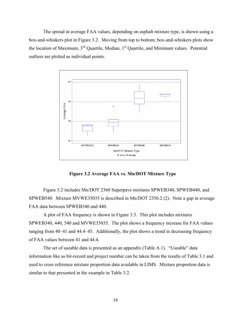
The spread in average FAA values, depending on asphalt mixture type, is shown using a
box-and-whiskers plot in Figure 3.2. Moving from top to bottom; box-and-whiskers plots show
the location of Maximum, 3rd Quartile, Median, 1st Quartile, and Minimum values. Potential
outliers are plotted as individual points.
Figure 3.2 Average FAA vs. Mn/DOT Mixture Type
Figure 3.2 includes Mn/DOT 2360 Superpave mixtures SPWEB340, SPWEB440, and
SPWEB540. Mixture MVWE35035 is described in Mn/DOT 2350.2 (2). Note a gap in average
FAA data between SPWEB340 and 440.
A plot of FAA frequency is shown in Figure 3.3. This plot includes mixtures
SPWEB340, 440, 540 and MVWE35035. The plot shows a frequency increase for FAA values
ranging from 40–41 and 44.4–45. Additionally, the plot shows a trend in decreasing frequency
of FAA values between 41 and 44.4.
The set of useable data is presented as an appendix (Table A.1). “Useable” data
information like as bit-record and project number can be taken from the results of Table 3.1 and
used to cross reference mixture proportion data available in LIMS. Mixture proportion data is
similar to that presented in the example in Table 3.2.

17
0
1
2
3
4
5
6
7
8
9
39.9 40.4 40.9 41.4 41.9 42.4 42.9 43.4 43.9 44.4 44.9 45.4 45.9 46.4 46.9 47.4
Average Mn/DOT FAA
Freq
uenc
y
Figure 3.3 Histogram: Frequency of Average Mn/DOT FAA Values
Table 3.2 Typical Project Mixture Proportion Data (LIMS)
P_BITREC Product Source, (Material Type) Mn/DOT Product ID
Specific Gravity Proportion
1 Pit A, FA-3 (GRANITE) #7312402818390 2.711 19
2 Pit A, CA-50 (GRANITE) #7312402818390 2.729 23
3 Pit A, WASHED SAND (GRANITE) #7312402818390 2.682 26
4 Pit B, MILLINGS #2711902223133 2.6 15
5 Pit C, WASHED SAND (LIMESTONE) #1902702433230 2.71 12
0-2001-XXX
6 Pit D, WASHED SAND #7103302621118 2.648 5
Mixture Information OLDREC WTDSPG VNEW AC % VOIDS % VMA % AC
0-2001-YYY 2.687 4.5 4 14 5.3

18
CHAPTER 4: ANALYSIS OF MEASURED FAA DATA
4.1 Introduction The Superpave Fine Aggregate Angularity (FAA) requirement is one of the aggregate consensus
properties recommended by the Strategic Highway Research Program (SHRP), and is outlined in
the Asphalt Institute publication; Superpave Series No. 2 (SP-2) (1). The uncompacted void
content of an aggregate is used as an indicator of FAA because aggregates with greater
angularity should likewise have greater uncompacted void content values. A standard test
method (AASHTO T304, ASTM C1252) is used to determine the void content.
The Uncompacted Void Content for FAA is determined by sieving and then
proportioning a washed sample of aggregate into the 190-g gradation indicated in Table 4.1.
Table 4.1 FAA test gradation requirements (13)
Sieve Mass (g) retained for AASHTO T 304 # 8 (2.36 mm) None, but material must pass this sieve. # 16 (1.16 mm) 44 ± 0.2 # 30 (0.6 mm) 57 ± 0.2 # 50 (0.3 mm) 72 ± 0.2
# 100 (0.15 mm) 17 ± 0.2 The test method includes running the 190-g sample through a funnel-to-cylinder
apparatus as pictured in Figure 4.1. Calculating FAA requires knowledge of the aggregate bulk
specific gravity (Gsb), the measured aggregate mass in the cylinder after striking off (Maggregate),
ρwater (1g/ml), and the volume of the cylinder (Vcylinder = 100 ml recommended).
FAA = % Uncompacted Voids =
( ) 100V
GsbMV
100V
VV
cylinder
water
aggregatecylinder
cylinder
stonecylinder ××ρ−
=×−
(1).

19
Figure 4.1 Standard testing apparatus for AASHTO T304, ASTM C1252 Method A
SP-2 recommends FAA values that correspond to design traffic and position within the
pavement structure. Table 4.2 reproduces that recommendation.
Table 4.2 Fine Aggregate Angularity Criteria (1)
FAA Requirements Depending on Depth from Surface Traffic, million ESALs < 100 mm > 100 mm
< 0.3 < 1 < 3 < 10 < 30 < 100 ≥ 100
- 40 40 45 45 45 45
- -
40 40 40 45 45
The State of Minnesota uses Standard Specification for Construction 2360 for Superpave
mixture design (2). Section 2360.2D2 corresponds to the SP-2 FAA requirements in stating that
ASTM C1252 Method A shall be used to evaluate the composite blend according to Table 4.3.
Traffic levels 2–7 are also defined.

20
Table 4.3 Minnesota FAA Specification 2360.2D2 for Traffic and Layer Depth (2)
Depth of Pavement from Surface
≤ 100 mm (4 inch) > 100 mm (4 inch) & Shoulders
Mn/DOT Traffic Level
(million ESALs) Minimum FAA (%) Minimum FAA (%)
Level 2 ( 0.3 ≤ 1) - Level 3 (1 ≤ 3) 40 40 Level 4 (3 ≤ 10) - Level 5 (10 ≤ 30) 45 40 Level 6 (30 ≤ 100) - Level 7 (> 100) 45 45
4.2 Aggregate Materials Aggregate materials were obtained from Minnesota Department of Transportation
(Mn/DOT) offices and donated from various private sources. Several districts and contractors
were able to supply aggregate samples appropriate for the study. Not all aggregates were used
during the mixture design phase. Omission was not a reflection on the aggregate quality, but
appropriateness for mixture comparison with respect to regional origin, quantity available, and
FAA. Material sources and descriptions are presented in Table 4.4.
Table 4.4 Aggregate materials included in Mn/DOT FAA validation study
Aggregate Source Size Type Supplier D1 Glacier Pit ½-in. minus Pit gravel Mn/DOT D1 D2 J & S Pit No. 4 minus Pit gravel Mn/DOT D2
SP Spilman 3/8-in. minus Pit gravel Mn/DOT D3
RI Ringo Pit 3/8-in. minus Pit gravel Mn/DOT D6 BA ½ Barton ½-in. minus Pit gravel Commercial Asphalt
DCF Danner No. 4 minus Danner Crushed Fines MnROAD stockpile
OP Otto Ped Sand No. 4 minus Natural sand MnROAD stockpile SL Unknown No. 4 minus Natural sand U of M stockpile
NU New Ulm Quarries No. 4 minus Manufactured quartzite sand NUQQ stockpile
NE Aggregate Industries – Nelson No. 4 minus Manufactured
sand U of M lab stockpile
KLS Kraemer No. 4 minus Manufactured lime sand Contractor stockpile
K 9/16 Kraemer 9/16-in. Limestone chips Contractor stockpile
21
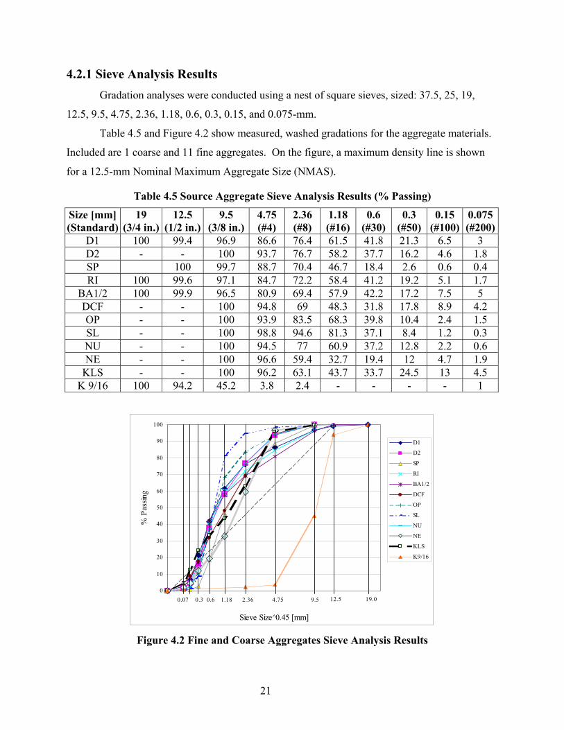
4.2.1 Sieve Analysis Results Gradation analyses were conducted using a nest of square sieves, sized: 37.5, 25, 19,
12.5, 9.5, 4.75, 2.36, 1.18, 0.6, 0.3, 0.15, and 0.075-mm.
Table 4.5 and Figure 4.2 show measured, washed gradations for the aggregate materials.
Included are 1 coarse and 11 fine aggregates. On the figure, a maximum density line is shown
for a 12.5-mm Nominal Maximum Aggregate Size (NMAS).
Table 4.5 Source Aggregate Sieve Analysis Results (% Passing)
Size [mm] (Standard)
19 (3/4 in.)
12.5 (1/2 in.)
9.5 (3/8 in.)
4.75 (#4)
2.36 (#8)
1.18 (#16)
0.6 (#30)
0.3 (#50)
0.15 (#100)
0.075(#200)
D1 100 99.4 96.9 86.6 76.4 61.5 41.8 21.3 6.5 3 D2 - - 100 93.7 76.7 58.2 37.7 16.2 4.6 1.8 SP 100 99.7 88.7 70.4 46.7 18.4 2.6 0.6 0.4 RI 100 99.6 97.1 84.7 72.2 58.4 41.2 19.2 5.1 1.7
BA1/2 100 99.9 96.5 80.9 69.4 57.9 42.2 17.2 7.5 5 DCF - - 100 94.8 69 48.3 31.8 17.8 8.9 4.2 OP - - 100 93.9 83.5 68.3 39.8 10.4 2.4 1.5 SL - - 100 98.8 94.6 81.3 37.1 8.4 1.2 0.3 NU - - 100 94.5 77 60.9 37.2 12.8 2.2 0.6 NE - - 100 96.6 59.4 32.7 19.4 12 4.7 1.9
KLS - - 100 96.2 63.1 43.7 33.7 24.5 13 4.5 K 9/16 100 94.2 45.2 3.8 2.4 - - - - 1
0
10
20
30
40
50
60
70
80
90
100
Sieve Size^0.45 [mm]
% P
assin
g
D1
D2
SP
RI
BA1/2
DCF
OP
SL
NU
NE
KLS
K9/16
19.012.5 9.5 4.75 2.36 1.18 0.60.07 0.3
Figure 4.2 Fine and Coarse Aggregates Sieve Analysis Results

22
4.2.2 Properties of Aggregates and FAA Analysis Results Aggregate Bulk (dry) Specific Gravity (Gsb), Apparent Specific Gravity (Gsa), and
absorption values are used in asphalt mixture analysis and design, and for determining the FAA
of a particular material. Recall the general definition of specific gravity:
water
material
waterof volumeequal
material
γγ
MM
Gs == (16).
Where γ is unit weight (weight/volume)
Apparent specific gravity differs from the bulk (dry) specific gravity according to how γ
material is defined. Roberts, et al. (5), provides the following definitions:
γ Apparent = Ws/Vs+ip
and
γ Bulk = Ws/(Vs+ip + Vpp).
Where Ws is the oven-dry sample weight, Vs+ip is volume of solids plus impermeable voids, and
Vpp is volume of water-permeable voids.
Roberts also defines percent absorption as Absorbed Water Weight/Ws.
Specific gravity measurements were performed on fine and coarse materials in
accordance with Mn/DOT Modified AASHTO T84 and T 85 (14, 15), respectively. Coarse and
fine materials are defined by the Mn/DOT Lab Manual, sections 1204.1 and 1205.1. The
definitions state that material passing 4.75-mm shall be called fine and material retained on the
4.75-mm [#4] sieve shall be called coarse. Results are presented in Table 4.6.
As seen previously, Minnesota Superpave 2360 FAA (% Uncompacted Voids)
specifications range from 40 to 45. FAA measurements of these 11 source materials ranged from
38.8 to 47.9. Materials having measured values outside the specification may be useable as
components of composite aggregate blends.

23
Table 4.6 Aggregate Specific Gravity, Absorption, and % Uncompacted Voids (FAA)
Aggregate Gsb Gsa % Absorption % Uncompacted Void Content
D1 2.667 2.799 1.626 41.1 D2 2.670 2.705 0.482 39.9
D3 (SP) 2.600 2.655 0.786 38.7 D6 (RI) 2.520 2.654 1.999 38.9 BA ½ 2.622 2.683 0.867 40.8 DCF 2.637 NA NA 47.8 OPS 2.622 NA NA 38.8 SL 2.620 2.691 1.010 39.7 NU 2.599 2.635 0.523 46.5 NE 2.667 2.783 1.564 46.9
KLS 2.710 2.782 0.951 47.9
K 9/16 2.645 2.820 2.340 NA – coarse aggregate
4.3 FAA Sensitivity to Physical Conditions The “angularity” of a particular aggregate grain may be regarded as fixed as long as no
action is taken to change the grain shape. However, since the testing process includes interaction
between the sample and testing apparatus, the possibility of measuring misrepresentative FAA
values exists. This interaction is partially represented in the Figure 4.3. The diagram of the
aggregate sample shows the external forces present during FAA testing. In addition to the
external gravitational and friction forces there are internal forces. Internal forces may vary with
aggregate material. The significance of these interactions is beyond the scope of this study.
Figure 4.3 External forces acting on FAA sample

24
Aggregate material slides through a metal funnel having a fixed opening, drops a short
distance then finally lands in a metal cylinder. Two nonstandard experiments were performed to
evaluate the influence of the drop height on FAA and to measure the duration of the test.
4.3.1 Drop Height Experiment The first experiment was conducted to estimate how FAA is sensitive to the testing
configuration. Measurements of the standard FAA testing configuration showed that the
standard drop distance is approximately 197-mm. In this experiment the drop distance from
funnel tip to the cylinder bottom was varied from this standard distance. Several things were
evident:
• for all drop heights; materials maintained an angularity order,
• angularity values decreased as the drop height distance increased, and
• high FAA (manufactured) materials tended to remain above 45.
FAA values were measured for distances from 100–444-mm. This interval is near the
practical limit since funnel-cylinder crowding occurs <100-mm and all of the aggregate may not
fall directly into the cylinder at distances >444-mm. Results of the test are observed in Figure
4.4. The best-fit lines on Figure 4.4 show that FAA changes slowly with respect to drop height.
y = -0.0059x + 48.995R2 = 0.9844
y = -0.0039x + 39.327R2 = 0.8212
37
39
41
43
45
47
49
100 200 300 400
DROP DISTANCE [mm]
FAA
D1
D2
SP
RI
DCF
KLS
NU
NE
OP
SL
Figure 4.4 FAA vs. Aggregate Drop Distance for modified AASHTO T304.

25
4.3.2 Timing Experiment A second nonstandard experiment was conducted to find out if the flow time of a 190-g
FAA sample is related to the sample FAA.
FAA is used to estimate the ability of an asphalt mixture to resist rutting deformation in
the field. In addition to high angularity, rut resistant aggregates may have form and surface
texture qualities that promote high internal friction.
The standard FAA test occurs in a controlled manner, with three basic external forces as
shown in Figure 4.5. Internal forces are also present but they may vary from material to material
because of angularity, form, or texture. The timing test is used here as an indirect indicator of
these properties; much as the Uncompacted Void Content indirectly indicates angularity.
Flow timing was measured using a stopwatch, standard 190-g FAA samples, and standard
FAA testing apparatus. Five time measurements per sample were obtained for averaging. For the
purpose of this experiment, flow time duration is defined as beginning with funnel opening and
ending when the last aggregate particle exits the funnel.
y = 5.4978x + 12.098R2 = 0.9106
35
40
45
50
4.5 5 5.5 6 6.5 7
FAA TIME [sec]
FAA
Figure 4.5 FAA vs. FAA Flow Time

26
The graphical results presented in Figure 4.5 show that flow time correlates well to FAA
for these 11 Minnesota aggregate materials. Flow times ranged from 4.8 to 6.6 seconds, with
higher flow time corresponding to higher FAA material. This trend gives confidence to the
standard FAA measurements and may be useful in the analysis of mixture performance.
4.4 Aggregate Imaging Systems (AIMS) The characterization of aggregates by digital imaging techniques was not part of the
project work plan. However, this additional work was later included because the research team
thought this analysis would be beneficial for the project; taking into consideration the fact that
AIMS has received considerable attention at the national level.
Samples of eight of the Minnesota aggregates were sent to the Civil Engineering
Department at Texas A&M University (TAMU), where digital imaging was performed.
4.4.1 AIMS Description and Definitions An Aggregate Imaging System (AIMS) is described in the work of Fletcher (9) and Al–
Rousan (10) as a digital imaging system that includes digital cameras, microscopes, top and back
lighting systems, and 3-dimensional motion actuators for analysis of coarse and fine aggregates.
Black and white images capture angularity and grey images capture texture. The testing
procedure includes:
• Aggregate placed on tray. Backlighting is used.
• A video microscope or video camera collects images of aggregate. Servo actuators control
the camera position relative to the x, y, or z-axis. The z-location depends on resolution
criteria. Resolution is based on the number of pixels available to image a particle.
• A row and column type scan is conducted in the x-y plane. Images of particles are included
in subsequent analyses based on resolution criterion.
Fine aggregate data is analyzed for angularity and form.
Angularity – Uses two methods:
1. Gradient Method uses an average of the difference between gradient vectors.
∑−
==θ−θ
−=
3N
1i3ii
13N
1Gradient (10).

27
Where N = number of edge points on particle, θ is the gradient vector, and i is the edge point.
The drawing in Figure 4.6 represents gradient vectors located at such an edge point on a 2-
dimensional projection of an aggregate particle.
Figure 4.6 Gradient Vectors (circled) at Particle Edge Point
2. Masad’s Radius Method uses the equation: ∑−
=355
0 θ
θθ
EE
EE
RRR
AI (9,10).
Where REEθ is the radius of an equivalent ellipse and Rθ is the particle radius at angle θ. Figure
4.7 shows the projection of an elongated particle and equivalent ellipse. The dotted line with
large arrowhead shows Rθ while the solid line and small arrowhead shows REEθ.
Figure 4.7 Radii on Partical and Equivalent Ellipse Projections (Radial Angularity)
Form
The Form Index for fine aggregates is based on a 2-dimensional projection of the aggregate
image. ∑θ∆−=θ
=θ θ
θθ∆=θ −=−
360
0 RRRForm D2 (10).
Where Rθ is the radius in a given direction and directional angle is given as angle θ.
2-D Form Index will equal 0 for a perfect circle. The drawing Figure 4.8 shows one set
of radii that contribute to the Form Index.

28
Figure 4.8 Radii Used for Calculating 2-D Form
4.4.2 Sample Preparation Aggregates were washed on the #200 sieve and separated by sieve analysis using a nest
of sieves having square opening sizes: 9.5, 4.75, 2.36, 1.18, 0.6, 0.3, 0.15, and 0.075-mm.
50-g of material retained on each sieve from 0.075–4.75-mm was individually packaged,
marked, and sent to Texas A&M for AIMS testing.
4.4.3 AIMS Results Figures 4.9–4.11 show AIMS results for eight of the Minnesota aggregates described in
section 4.2. These figures include angularity and form measurements on 50-g samples of
material retained on the 2.36 (#8) and 1.18-mm (#16) sieves.
Figure 4.9 (Gradient Angularity) shows how angularity varies for each sample. Lower-
angularity materials plotted on the left side of the group. At 100% of particles measured,
gradient angularity values vary from approximately 5000 to a maximum of 10000.
Figure 4.10 (Radial Angularity) shows how angularity varies for each sample. Lower-
angularity materials plotted on the left side of the group. Minimum values for all material are
near 3 or 4. At 100% of particles measured, radial angularity measurements are spread from
approximately 10 to 20.
Figure 4.11 (2-D Form) shows how shape varies for each sample. Materials having a
more rounded shape are plotted on the left side of the group. Minimum values for all materials
are near 3, indicating that a few particles in each sample project a nearly circular area. At 100%
of particles measured, 2-D form measurements are spread from approximately 10 to 18.

29
0
10
20
30
40
50
60
70
80
90
100
500 1500 2500 3500 4500 5500 6500 7500 8500 9500
Gradient Angularity
% o
f Par
ticle
s
D1 #8 D1 #16D2 #8 D2 #16SP #8 SP #16RI #8 RI #16BA1.2 #8 BA1/2 #16KLS #8 KLS #16NE #8 NE #16NU #8 NU #16
Figure 4.9 AIMS Gradient Angularity for 8 Minnesota Aggregates
0
10
20
30
40
50
60
70
80
90
100
3 5 7 9 11 13 15 17 19 21
Radius Angularity Index
% o
f Pas
sing
D1#8 D1#16 D2 #8
D2 #16 SP #8 SP #16
RI #8 RI #!6 BA1/2 #8
BA1/2 #16 KLS #8 KLS #16
NE #8 NE #16 NU #8
NU #16
Figure 4.10 AIMS Radial Angularity for 8 Minnesota Aggregates

30
0
10
20
30
40
50
60
70
80
90
100
3 5 7 9 11 13 15 17 19
Form 2D Index
% o
f Par
ticle
s
D1 #8 D1 #16 D2 #8
D2 #16 SP #8 SP #16
RI #8 RI #16 BA1/2 #8
BA1/2 #16 KLS #8 KLS #16
NE #8 NE #16 NU #8
NU #16
Figure 4.11 AIMS 2-D Form for 8 Minnesota Aggregates
Figures 4.12–4.16 show typical black and white imaging data for several unblended
aggregates. This type of data is used in the process of evaluating angularity and 2-dimensional
form.
Figure 4.12 Image of SP (FAA 37.8)
Figure 4.13 Image of RI (FAA 38.9)

31
Figure 4.14 Image of BA1/2 (FAA 40.8)
Figure 4.15 Image of NE (FAA 46.9)
Figure 4.17 Image of KLS (FAA 47.9)

32
CHAPTER 5: DEVELOPMENT OF A LABORATORY TESTING
PROGRAM
5.1 Introduction A laboratory testing program was developed for Fine Aggregate Angularity (FAA)
validation based upon the following criteria.
In order to reduce the number of factors that affect mixture properties and emphasizing
the role of FAA:
1. With the exception of FAA, mixtures shall be designed to Mn/DOT 2360 Superpave
specifications (2). If possible, the range of composite blend FAA values in the testing
program shall be designed both above and below the Mn/DOT 2360 Superpave
specifications.
2. The number of variables shall be minimized in order to see the effect of FAA. Mixtures shall
have similar gradations and void content. A single performance-graded asphalt binder shall
be used. Voids Filled with Asphalt (VFA) and Voids in Mineral Aggregate (VMA) shall
meet Mn/DOT 2360 requirements.
3. The testing regimen shall include aggregate and mixture evaluation. Aggregate evaluation
includes sieve analysis, specific gravity, and FAA for component aggregates and the
composite blends. Mixture evaluation includes dynamic modulus (|E*|) testing at appropriate
conditions and rutting performance testing. |E*| data corresponding to high temperatures
shall be useful since mixtures are more sensitive to rutting at high temperatures. The
principle of time-temperature superposition can be used to show how high temperature
relates to low frequency modulus values.
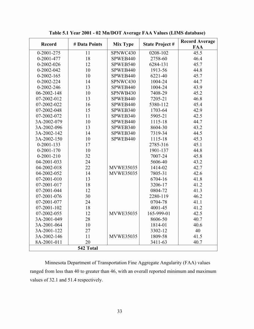
5.2 Range of FAA values With reference to Chapter 2: it was possible to break down Mn/DOT reported FAA
values and average them so they correspond with State Project Number, mixture type, and
record number. Table 5.1 shows 34 such averaged values.
33
Table 5.1 Year 2001 - 02 Mn/DOT Average FAA Values (LIMS database)
Record # Data Points Mix Type State Project # Record Average FAA
0-2001-275 11 SPNWC430 0208-102 45.5 0-2001-477 18 SPWEB440 2758-60 46.4 0-2002-026 12 SPWEB540 6284-131 45.7 0-2002-042 10 SPWEB440 1913-56 44.8 0-2002-165 10 SPWEB440 6221-40 45.7 0-2002-224 14 SPNWC430 1004-24 44.7 0-2002-246 13 SPWEB440 1004-24 43.9 06-2002-148 10 SPNWB430 7408-29 45.2 07-2002-012 13 SPWEB440 7205-21 46.8 07-2002-022 16 SPWEB440 5380-112 45.4 07-2002-048 15 SPWEB340 1703-64 42.9 07-2002-072 11 SPWEB340 5905-21 42.5 3A-2002-079 10 SPWEB440 1115-18 44.7 3A-2002-096 13 SPWEB340 8604-30 43.2 3A-2002-142 14 SPWEB340 7319-34 44.5 3A-2002-150 10 SPWEB440 1115-18 45.3 0-2001-133 17 2785-316 45.1 0-2001-170 10 1901-137 44.8 0-2001-210 32 7007-24 45.8 04-2001-033 24 5606-40 43.2 04-2002-018 22 MVWE35035 1414-02 42.7 04-2002-052 14 MVWE35035 7805-31 42.6 07-2001-010 13 6704-16 41.8 07-2001-017 18 3206-17 41.2 07-2001-044 12 0804-72 41.3 07-2001-076 30 2280-119 46.2 07-2001-077 24 0704-78 41.1 07-2001-102 18 4001-45 41.2 07-2002-055 12 MVWE35035 165-999-01 42.5 3A-2001-049 28 8606-50 40.7 3A-2001-064 10 1814-01 40.6 3A-2001-122 27 3302-12 40 3A-2002-146 11 MVWE35035 1809-58 41.5 8A-2001-011 20 3411-63 40.7
542 Total
Minnesota Department of Transportation Fine Aggregate Angularity (FAA) values
ranged from less than 40 to greater than 46, with an overall reported minimum and maximum
values of 32.1 and 51.4 respectively.

34
The project committee recommended that FAA composite-blend values should be
designed both above and below the Mn/DOT 2360 Superpave FAA specifications, if possible.
All other aspects of the mixtures should conform to 2360 criteria.
Table 5.2 shows that recent Mn/DOT project reports do not indicate construction having
FAA values below 40. The aggregate gathered for study is similar in range to Mn/DOT records,
with a somewhat smaller median. This comparison also shows that in order to measure below
the FAA minimum, a mixture would likely include high proportions of the aggregates that fall
into the first quartile.
Table 5.2 FAA Comparison: Mn/DOT Mixtures (Table 5.1) and Available Aggregate
Min. Quartile 1 Median Quartile 3 Max. 2001-02 Mn/DOT Records
(34 mixture) 40 41.6 43.6 45.3 46.8
Available FAA –Aggregate (11 fine components) 38.7 39.3 40.8 46.7 47.9
Mn/DOT FAA Specification 2360 40 - - - 45
Committee and project staff agreed to develop a total of four asphalt mixtures. Of the
four mixtures, two should have high FAA and two should have low FAA measurements. The
minimum material required to design four mixtures was one coarse aggregate and four fine
aggregates, as long as 2360 requirements were satisfied. The Chapter 5 report will present
aggregates the blend design process.
5.3 Mixture Design Mixture design must meet the Mn/DOT 2360 Superpave criteria. Since all aggregate
materials were obtained from reputable known sources and are normally approved for mixture
design, they were assumed to possess adequate toughness and soundness. The design process
could then focus mainly on FAA, gradation, and optimum asphalt content.
To expedite design, gyratory compaction levels were recommended by the Mn/DOT
Bituminous Office. The high-FAA mixtures would follow traffic level 4 and the low-FAA
mixtures would follow traffic level 3 as listed in Table 2360-7.
The mix design procedure is described below:
1. Gradation design. All gradations have:

35
• A single PG58-28 asphalt binder
• Nominal Maximum Aggregate Size of 12.5 mm
• No more than three aggregate components; 1 coarse and 1–2 fine
• A single coarse aggregate material was used for all blends, and in the same (approximate)
proportion
• Fine aggregate material consisted of the study aggregate (2 high, 2 low FAA) and, if
needed, a second (low FAA) aggregate.
2. Mixture design specimens were two identical 4800-g specimens, having a diameter of 150-
mm, per design iteration. Compaction was carried out on a Brovold Gyratory Compactor at
600-kPa and gyration angle of 1.25 degrees.
3. Optimum asphalt content determination using 4800-g specimens.
• Vary asphalt content
• 96% Gmm at Ndesign
• 97% Gmm at Nmaximum
4. Final designs satisfied Mn/DOT 2360 design criteria.
5.4 Dynamic Modulus Test Dynamic modulus |E*| testing was used to determine the rut resistance of each mixture.
This approach is based on previous research performed by T. Pellinen and M. Witczak that
showed that |E*| correlates to mixture rutting. The testing regimen required four 100-mm
(diameter) by 150-mm (height) cylindrical cored specimens per mixture design. Each specimen
was cut and cored from a 150-mm by 170-mm cylinder. All specimens were produced at 95%
Gmm in the Brovold Gyratory Compactor at 600-kPa and gyration angle of 1.25 degrees.
Modulus testing was carried out using a MTS load frame.
Dynamic modulus testing included 3 temperature conditions with 5 frequencies per
temperature condition. Temperatures of 20, 40, and 54C were chosen since the binder material
used was PG58-28. Frequencies of 25, 10, 1, 0.1, and 0.01 Hz were used for 20 and 40C. At 54C
the same set of frequencies was used; however 0.01 Hz was excluded because of difficulty in
measuring high frequencies at high temperatures.

36
5.5 Rut Susceptibility Testing Rut development analysis was done using the Asphalt Pavement Analyzer (APA). APA
testing was included as a means of ranking mixtures according to performance. This testing
setup required 150-mm (diameter) by 75-mm (height) cylindrical specimens. Two APA
specimens were cut from a single gyratory-compacted cylindrical specimen (150-mm by 170-
mm). APA specimens were produced at 95% Gmm in the Brovold Gyratory Compactor at 600-
kPa and gyration angle of 1.25 degrees.
APA testing included two APA specimens per mixture design. The specimens were
tested at a temperature of 54C for comparison with dynamic modulus results. Figure 5.1 shows
the basic APA testing setup. Test components include an automated rolling wheel applying a
445-N (100-lb) load while moving along a hose pressurized to 700-kPa (100-psi).
Figure 5.1 APA Testing Setup. Asphalt specimen below pressure hose and roller.

37
CHAPTER 6: LABORATORY MIXTURE DESIGN
6.1 Introduction Chapter 5 (Development of Laboratory Testing Program) described points from which
the FAA validation testing program was developed. Development of the mixture design portion
of the FAA validation study was based upon several points:
1. With the exception of FAA criteria, asphalt mixtures should be designed to Mn/DOT 2360
specifications (2).
2. Mixtures should have similar gradations and void content. A single performance-graded
asphalt binder should be used. Voids Filled with Asphalt (VFA) and Voids in Mineral
Aggregate (VMA) should meet Mn/DOT 2360 requirements.
3. The testing regimen should include aggregate and mixture evaluation.
With reference to Chapter 3: it was possible to break down Mn/DOT reported FAA values
and average them so they correspond with State Project Number, mixture type, and record
number. Since all aggregate materials were obtained from reputable known sources and are
normally approved for mixture design they were assumed to possess adequate toughness and
soundness. The design process could then focus mainly on FAA, gradation, and optimum
asphalt content.
Final mixture designs (Chapter 6) for validating Fine Aggregate Angularity (FAA) were
the culmination of several points:
1. Mixtures included aggregate materials representative of Minnesota. Some aggregate
materials presented in Chapter 4 (Analysis of FAA Data) were obtained from several
Mn/DOT district offices. Other aggregate materials were also obtained from the Metro area
and greater Minnesota. A total of one (1) coarse and eleven (11) fine aggregate materials
were available for use in this study.
2. Materials used should display low, medium, and high FAA in composite blends. Chapter 5
compared FAA values for available aggregates, past Mn/DOT mixture data, and Mn/DOT
specifications. Table 4.1 showed that in order to measure below the FAA minimum, a
mixture would probably include high proportions of the aggregates having FFA from the
minimum to the first quartile. Five (5) fine aggregate materials measured below FFA 40.

38
3. Mixtures were designed with current Minnesota Superpave volumetrics (2). A 12.5-mm
Nominal Maximum Aggregate Size (NMAS) was used. Mn/DOT Specifications, Table
2360-2 (2) contains gradation limits for Superpave mix designs. Percent mixture in the
“FAA band” may be determined, and is noted below in Table 6.1. “FAA band” is defined as
the material passing the 2.36-mm (#8) sieve and retained on 0.300 (#50).
Table 6.1 Percent of Mn/DOT 2360 Mixture Located in FAA Band (2)
Mixture NMAS % of Mn/DOT Mix in FAA Band 9.5 mm 27.05 – 53.20 12.5 mm 23.44 – 45.08 19 mm 18.93 – 37.87
For purposes of comparison, FAA percentages for other Mn/DOT asphalt mixture
designs are given in Table 6.2, taken from Mn/DOT Specifications, Table 3139-1 (2).
Table 6.2 Percent of Mixture Located in FAA Band (2)
Mn/DOT Mixture Type % of Mix in FAA Band
31&32 A 23.32 – 47.25 31&32 B 23.32 – 47.25 31&32 C 23.32 – 47.25 41&42 A 23.32 – 47.25 41&42 B 23.32 – 47.25 47&48 A 23.32 – 47.25 47&48 B 23.32 - 41.11
61 CC, CS WEAR 20.70 – 47.86 61 CC, CS NONWEAR 20.70 – 47.86
61 TT WEAR 34.98 – 57.07 61 TT NONWEAR 34.98 – 57.07
Specification 2360 section F3 to F5 presents a set of volumetric Voids in Mineral
Aggregate (VMA), and Voids Filled with Asphalt (VFA) criteria for mixture design.
• 2360 F3 states that mixture design air voids at Ndesign should equal 4% for those mixtures
placed above a 100-mm final depth and 3% for mixtures placed below. For the purposes
of this FAA study the 4% at Ndesign criterion was used.

39
• 2360 F4 specifies VMA criteria for 9.5, 12.5, and 19.0-mm Nominal Maximum
Aggregate Size (NMAS). For the purposes of this FAA study the 12.5-mm NMAS
criteria was used. Summarizing:
• Fine mixtures (>39% passing 2.36-mm (#8) sieve) having 12.5-mm NMAS require a
minimum 14% VMA. Corresponding coarse mixtures require a minimum 13.5% VMA.
2360 F5 specifies VFA criteria for traffic levels. For this FAA study, the project committee suggested traffic levels 3 and 4. Summarizing;
• Traffic level 3 requires 65–78 % design VFA for mixtures placed below a 100-mm final
depth. Traffic level 4 requires 65–75% design VFA for mixtures placed below a 100-mm
final depth.
4. Performance graded asphalt binder, appropriate for Minnesota climate, shall be used. For the
purposes of this project, and for comparison with other Mn/DOT-sponsored projects, a Koch
PG58-28 unmodified asphalt binder was used.
5. No recycled material was included in this study.
6.2 Mixture Design Material Aggregate materials included in trial mixtures were selected according to FAA
measurement, ability to represent a Minnesota region, and quantity available. Available material
is listed below in Table 6.3. As stated in Chapter 4, not all aggregates were used during the
mixture design phase. However, omission is not a reflection on the aggregate quality or general
usefulness in bituminous mixtures. Inclusion was based on appropriateness for mixture
comparisons, variety of regional origin, quantity available, and FAA.

40
Table 6.3 Material Available for FAA Study
Material Description Quantity Comments Trial Mix
Asphalt Binder Koch PG58-28 NA Yes Coarse Aggregate Kraemer 9/16 Lime Chips 1000 kg Yes
D1 ½-in. minus (Glacier) FAA 41.1
50 kg Low-FAA (NE MN) AIMS Data
No
D2 No. 4 minus (J&S) FAA 39.9 75 kg
Low-FAA (NW MN) AIMS Data
No
SP 3/8-in. minus (Spilman) FAA 38.7 75 kg
Low-FAA (NW MN) AIMS Data
Yes
RI 3/8-in. minus (Ringo) FAA 40.8 100 kg
Low-FAA (S MN) AIMS Data
Yes
BA½ ½-in. minus (Barton) FAA 40.8
500 kg Low-FAA (Metro) contributes P200 AIMS Data
Yes
DCF No. 4 minus (Danner) FAA 47.8 20 kg High-FAA
(Metro) No
OP No. 4 minus (Otto Ped) FAA 38.8 20 kg Low-FAA
(Metro) No
No. 4 minus (U of M Lab) FAA 39.7 500 kg
Low-FAA (no region) AIMS Data
No
No. 4 minus (New Ulm) FAA 46.5 150 kg
High-FAA (S-Central MN) AIMS Data
Yes
No. 4 minus (Agg. Ind. NE) FAA 46.9 500 kg
High-FAA (Metro) AIMS Data
Yes
Fine Aggregate
KLS No. 4 minus (Kraemer) FAA 47.9 1000 kg High-FAA
(Metro) Yes
6.3 Trial Laboratory Mixtures 6.3.1 Mixture Production
Trial mixtures were produced using the following procedure:
• Select aggregate blend according to Mn/DOT Specification 2360 gradation bands in Figure 6.1. Calculate binder for several trial mixtures.

41
0
10
20
30
40
50
60
70
80
90
100
SIEVE OPENING [mm^0.45]
PER
CEN
T PA
SSIN
G
19.012.5 9.5 4.75 2.36 1.18 0.60.07 0.3
Figure 6.1 Mn/DOT 12.5-mm Mixture Design Gradation Band (2)
• Using ovens, heat enough aggregate and binder to produce two 4800-g gyratory specimens
and one 2000-g maximum specific gravity specimen at 145C (4 hours). Also heat mixing
tools.
• Combine coarse aggregate, fine aggregate and binder in bucket mixer, noting actual binder
added to mixture.
• Return mixture to ovens for aging at 135C (3 hours, stirring every hour). Heat gyratory mold,
plates, and tools. Lower temperature to 133C for compaction.
• Compact two specimens to Nmax for volumetric analysis. Compactor software records
specimen height and automatically generates an average densification curve using height and
estimated volumetrics (Gmm, Gmb).
• Obtain trial mixture volumetrics using Theoretical Maximum Specific Gravity (ASTM D
2041) and Bulk Specific Gravity of Compacted Specimens (ASTM D 2726) calculations as
follows:

42
Where C-BA
AGmm+
=
A = Oven dry mass of loose asphalt sample
B = Buoyant mass of pycnometer filled with water
C = Buoyant mass of pycnometer, mixture and water
WhereC-B
AGmb =
A = Oven dry mass of compacted specimen
B = Saturated surface dry mass of compacted specimen
C = Buoyant mass of compacted specimen
• Input volumetrics into the compaction curve estimate to obtain the corrected densification
curve.
• Evaluate trial mixture with VMA, VFA, Binder content, and air voids (Va) for particular
gyration levels Ninitial, Ndesign, and Nmaximum as follows:
GmmGmb-Gmm100Va =
GsbPsGmb100MAV ×
−=
VMAVa-VMA100VFA =
(1).
• Adjust mixture design by either altering the aggregate material, gradation blend, or binder
content. Best results were obtained when reserving binder content changes for fine
adjustments.
6.3.2 Mix Design Issues Mix design requires an understanding of volumetrics and how different factors affect
voids in the mixture. By far the most important issue in designing a good asphalt mixture is
selecting the proper aggregate structure. A large portion of the initial mix design process
included mixture blend improvement by process of trial and error.

43
High FAA Trial One:
The first trial mixture design used a blend of two high-angularity materials. The coarse
aggregate was 9/16 limestone chips (K9/16), and the fine aggregate was a 100% crushed,
manufactured sand (NE). Gradations for both materials are presented in Chapter 4. The
limestone material was basically a single size aggregate, with approximately 3% passing the
4.75-mm sieve. The NE sand was well graded, with a fine aggregate angularity (FAA) value of
46.9. Initial proportions were 35% limestone and 65% sand. With 5.4% asphalt binder, the
mixture had air voids of about 7.7% at Ndesign. 4.0% air voids were achieved at Ndesign by adding
7.4% asphalt binder. This drove the voids in mineral aggregate (VMA) to about 17% and the
voids filled with asphalt (VFA) to 76%. These values are significantly higher than what is
typically used in Minnesota.
Aggregate proportions were then changed in an attempt to improve mixture volumetrics.
A mix of 26% limestone and 74% sand and was produced at 6.0% asphalt. The air voids and
related parameters were still unreasonably high.
High FAA Trial Two:
A second aggregate combination was used to see if mixture volumetrics could be
improved. Trial two included 30% K9/16 with 70% washed limestone sand (KLS). The trial
two mixture yielded acceptable volumetric results. At 5.4% asphalt, the air voids were 4.0%, the
VMA was 14.1%, and the VFA was 72.3%. These satisfied specification limits and were
reasonable values for Minnesota mixtures. This mixture was the first selected for dynamic
modulus testing. This high-FAA trial mix will be referred to hereafter as “Mix 1 (KR)”.
The KLS sand and NE sands had similar gradations and FAA values. However, vastly
different mixture results were obtained.
High FAA Trial Three:
A high-angularity, quartzite sand with a FAA of 46.5 was evaluated. The gradation of
this material differed from the previous high-FAA sands. A mixture of 30% K9/16, 70%
quartzite sand and 5.0% asphalt yielded air voids of approximately 12% at Ndesign. These results
showed it was necessary to use other aggregate blends in order to satisfy the project volumetric
requirements.

44
High FAA Aggregate Blend Improvement:
The project technical support committee suggested including another aggregate product
in the design gradations. BA½ was obtained aid in our mix design. This product is a natural
gravel, and is well graded from the ½-inch (12.5-mm) to #200 (0.075-mm) sieve. The fine
portion had a FAA value of 40.8.
High FAA Trial Four:
A mixture was produced with 15% K9/16, 46% BA ½ inch, 39% NU sand, and 5.5%
asphalt binder. The mixture had approximately 76% passing the #4 sieve. Air voids were
measured at 11% at Ndesign, requiring additional blend adjustment.
High FAA Trial Five:
A mixture was produced with 20% K9/16, 50% BA ½ inch, 30% NE, and 5.6% asphalt
binder. Air voids measured 4% Ndesign. VMA and VFA values were within the specified range.
This high-FAA trial mix will be referred to hereafter as “Mix 2 (NE)”.
Design of Low FAA Aggregate Blends
While all of the high-FAA mixture blends fell within the specified gradation limits, the
mixtures often did not meet volumetric requirements. Plots of both acceptable high-FAA trial
blends fell close to the line of maximum density for a 12.5-mm NMAS. Bailey mixture design
coefficients were employed as a tool for further evaluating the high-FAA blends. These
coefficients were then used as a reference point for designing the low-FAA blends for “Mix 3
(RI)” and “Mix 4 (SP)”.
Description of Bailey Coefficients:
The Bailey method of asphalt mixture gradation design (3) analyzes packing
characteristics by dividing gradations into segments according to primary and secondary sieve
sizes and then forming coefficients based upon the aggregate proportions retained within those
particular segments. A range of values is recommended for each coefficient based upon design
experience.

45
Nominal Maximum Aggregate Size (NMAS) = one sieve size larger than the first sieve
that retains 10% or more of the material.
Table 6.4 Bailey Sieve Terminology (3)
SieveTerminology Definition Critical Sieve Sizes [mm] For 12.5 NMAS
Primary Control Sieve PCS = NMAS(0.22) 2.36mm Half Sieve HS = NMAS(0.5) 4.75mm
Fine Agg. Initial Break Sieve FAIB = PCS(0.22) 0.600mm Fine Agg. Secondary Break Sieve FASB = FAIB(0.22) 0.15mm
Bailey coefficients compare particular portions of gradations and are named: Coarse
Aggregate Ratio (CA), Coarse Fraction of Fine Aggregate (FA c), and Fine Fraction of Fine
Aggregate (FA f).
The four final FAA mixture design gradations are similar in that they fall within the
Specification 2360 gradation bands, stay close to the line of maximum density, and have similar
components. Low-FAA blends 3&4 were designed to stay near the line of maximum density and
have similar Bailey coefficients. Blend Bailey coefficients are given in the following table.
Some difference exists between high (1&2) and low angularity (3&4) blend CA coefficients.
Table 6.5 Composite Blend Coefficients for Four Asphalt Mixture Designs
Blend Coefficients Bailey Gradation Coefficient Definition
Suggested Range 1 (KR) 2 (NE) 3 (RI) 4 (SP)
CA = (%HS-%PCS) ÷ (100 - %HS) 0.4 - 0.8 0.76 0.70 0.21 0.20 FA c = %FAIB ÷ %PCS 0.25 - 0.5 0.52 0.48 0.61 0.49
FA f = %FASB ÷ %FAIB 0.25 - 0.5 0.30 0.18 0.19 0.13
6.4 Final Mixture Designs Table 6.6 presents the four final aggregate blends used for mixture design. Each blend
contains 20–30% of K 9/16, a poorly graded coarse material. Refer to Chapter 4 for sieve
analysis results covering individual aggregate products.

46
Table 6.6 Description and Proportions of Aggregates in Final Mixture Designs
Mixture Aggregate Proportions Aggregate Material Description Blend 1
(KR) Blend 2
(NE) Blend 3
(RI) Blend 4
(SP) KLS well graded manufactured sand 70%
K 9/16 poorly graded crushed rock 30% 20% 30% 30% NE poorly graded manufactured sand 30%
BA 1/2 well graded gravel 50% 40% 40% RI well graded gravel 30% SP well graded gravel 30%
Composite gradations were calculated from mixture proportions and individual sieve
analysis results. Results follow in Table 6.7 and are plotted in Figure 6.2.
Table 6.7 Mixture Design Composite Gradations
Sieve Size (mm) Blend 1 (KR) Blend 2 (NE) Blend 3 (RI) Blend 4 (SP) 19 100 100 100 100
12.5 98.3 98.8 98.1 98.2 9.5 83.6 85.3 81.3 82.1 4.75 68.5 69.2 58.9 60.1 2.36 44.5 47.7 50.3 52.1 1.18 30.2 33.8 41.2 41.1 0.6 23.0 23.1 30.5 25.5 0.3 16.3 9.4 14.4 8.3 0.15 6.9 4.1 5.6 3.4 0.075 2.2 2.9 3.5 2.6
6.4.1 Composite FAA Angularities by Measured and Calculated and Methods The scope of this study includes comparison of measured and calculated FAA values.
The Mn/DOT Lab Manual, section 1206, presents methods for proportioning individual
aggregate products and performing FAA measurements and calculations (4). Figure 6.3 shows
measured FAA values for the four mixture designs in relation to Superpave criterion (reference
Chapter 4). Knowing individual product proportions, FAA, Gsb, and gradation, it is possible to
calculate the FAA values of composite blends.

47
0
10
20
30
40
50
60
70
80
90
100
sieve opening^0.45
% P
assin
g
Blend 1KR(48.9)
Blend 2 NE(43.3)
Blend 3 RI(41.2)
Blend 4 SP(40.4)
19.012.5 9.5 4.75 2.36 1.18 0.60.075 0.3
Figure 6.2 12.5-mm NMAS Mixture Design Gradations, Blend FAA Value in Parenthesis
40 42.5 45 47.5 50
FAA
Superpave FAA Criterion
Mix 1
Mix 2
Mix 3
Mix 4
Figure 6.3 Measured FAA of Composite Gradations

48
It is possible to either calculate a proportion-weighted FAA value similar to an aggregate-
blend specific gravity calculation or a gradation-weighted average, as shown below:
Proportion-Weighted Blend Calculation
Blend∑
∑=
i
i
i
FAAP
PFAA
Gradation-Weighted Average Calculation
Blend ∑
∑×
××=
ii
iii
Fines%PFAAFines%P
FAA
Where:
Pi = Percent of component aggregate in mixture blend
FAAi = Component aggregate FAA
% Finesi = % of component aggregate passing the 4.75-mm (#4) sieve
Table 6.8 compares weighting methods by showing estimated and measured FAA values
for aggregate blends. The estimates are conservative since they do not take into account the
contribution of fines from crushed coarse aggregate K9/16. In this case only 3.8% of the high-
angularity K 9/16 material passes the 4.75-mm sieve and 2.4% passes the 2.36-mm (#8) sieve,
but nevertheless raises the composite blend angularity.
Table 6.8 Measured and Estimated FAA Values for Mixture Design Composite Blends
(FAA Validation)
Blend 1 (KR)
Blend 2 (NE)
Blend 3 (RI)
Blend 4 (SP) Average
Measured FAA 48.9 43.3 41.2 40.4 - Proportion-weighted Calculation
(% Error) 47.9
(2.04) 42.9
(0.92) 40.0
(2.91) 39.9
(1.24) -
(1.78) Gradation-weighted Calculation
(% Error) 47.9
(2.04) 43.3 (0)
40.0 (2.91)
39.9 (1.24)
- (1.55)
6.4.2 Composite Aggregate Imaging System (AIMS) Angularities The characterization of aggregates with digital imaging was not included as part of the
initial project work plan. It was included subsequent to the start of research in an effort to

49
compare conclusions about the effect of aggregate form and angularity on mixture performance.
Refer to Chapter 4 for a description of aggregate imaging data.
It was possible to proportion aggregate imaging data using nearly the same method used
for obtaining composite aggregate blends. Since no AIMS data existed for the coarse K9/16
material, it was necessary to modify the proportions of the remaining component materials
accordingly. This was done assuming that the coarse material made an insignificant contribution
to the amount retained on the 1.16-mm (#16) sieve. Recall that sieve analysis of the K9/16
reported 2.4% passing the 2.36-mm sieve, which would amount to less than 0.8% of the material
in the total aggregate blend.
Digital imaging quartile and median values were chosen for description since they offer a
robust means of evaluating data. The representative AIMS values are presented in Table 6.9.
Table 6.9 Blended AIMS Angularities
Minimum Quartile 1 Median Quartile 3 Maximum #16 Radial Angularity Blend 1 (KR) 3.30 5.89 7.39 9.66 17.71 Blend 2 (NE) 3.25 5.68 7.68 10.13 13.11 Blend 3 (RI) 3.08 5.35 6.80 8.71 11.95 Blend 4 (SP) 3.01 4.98 6.33 8.08 11.80 #16 Gradient Angularity Blend 1 (KR) 1631.45 2812.85 4135.01 5414.78 9001.35 Blend 2 (NE) 534.50 2587.82 4156.01 6209.48 8424.53 Blend 3 (RI) 594.75 2177.97 3423.64 4741.73 6911.58 Blend 4 (SP) 570.64 2129.73 3399.53 5392.71 7417.89 #16 Fines Form Blend 1 (KR) 4.16 6.67 7.94 9.47 13.41 Blend 2 (NE) 3.70 6.43 7.79 10.39 13.44 Blend 3 (RI) 3.21 5.77 6.76 9.00 12.40 Blend 4 (SP) 3.14 5.39 6.47 8.17 11.96

50
CHAPTER 7: FABRICATION AND TESTING OF HMA
SPECIMENS
7.1 Specimen Fabrication for Dynamic Modulus and Asphalt
Pavement Analyzer Testing Asphalt mixture rutting resistance is related to the internal friction provided by the
aggregate component. A total of sixteen cylindrical dynamic modulus specimens were produced
from four asphalt mixtures for the purpose of evaluating rutting resistance by dynamic modulus
(|E*|) testing. Additionally, a total of eight cylindrical specimens were produced from the same
four mixtures for evaluating rutting resistance with the Asphalt Pavement Analyzer (APA).
The four mixture designs were produced from one coarse material, four fine materials
typical of several Minnesota regions, and a fifth fine material used to improve the laboratory
mixture design. Source and manufacture method information is found in Chapter 4. Current
Mn/DOT specifications require FAA from 40–45. The range of measured composite blend FAA
values was 40.4 to 48.9.
7.1.1 Mixture Descriptions Mixtures 1 and 2 were designed using high-FAA materials while mixtures 3 and 4 were
designed with low-FAA materials.
• Mixture 1 included 2 aggregate materials, 30% crushed, coarse limestone and 70%
manufactured limestone sand (FAA = 47.9). Optimum asphalt was determined to be 5.5%.
• Mixture 2 included 3 aggregate materials, 20% crushed, coarse limestone, 50% bituminous
aggregate (FAA = 40.8), and 30% crushed granite (FAA = 46.9).
• Mixture 3 included 3 aggregate materials, 30% crushed, coarse limestone, 40% bituminous
aggregate (FAA = 40.8), and 30% natural gravel (FAA = 38.9).
• Mixture 4 included 3 aggregate materials, 30% crushed, coarse limestone, 40% bituminous
aggregate (FAA = 40.8), and 30% natural gravel (FAA = 38.7).
51
7.2 Dynamic Modulus Specimen Fabrication Steps Specimens were fabricated using the results from the trial mixture phase as reported in
Chapter 6. A total of four (4) 7200-g gyratory specimens were produced using NCHRP Project
9-29 procedures (18).
1. Measure two batches of aggregate proportioned for mixture blend. Each batch shall contain
enough material to produce two (2) 7200-g gyratory specimens. Place in oven along with
binder and mixing tools and heat at 145C for 4 hours.
2. Mix first batch of aggregate and binder in bucket mixer. Record binder measurement. Place
mix in pan. Repeat for second batch of aggregate and binder.
3. Mix both batches together. Measure out mixture for 4 specimens.
4. Place mixture in oven and age at 135C for 4 hours. Stir hourly. Last 30 minutes lower
temperature to 133C.
5. Compact cylindrical specimen (150 by 170-mm) to 5.5–6% air voids by trial and error using
a gyratory compactor.
6. Core and cut specimen produced in (5) to 100 by 150-mm cylinder.
7. Measure Gmb. Calculate void content, VMA, VFA. Void content of cut, cored specimen
should be 5%.
7.2.1 Dynamic Modulus Specimen Volumetric Documentation In preparation for dynamic modulus testing, the 150 by 170-mm gyratory specimens were
cored and cut to final dimensions of 100 by 150-mm. Tables 7.1 and 7.2 report averaged
measurements for each asphalt mixture.

52
Table 7.1 N-design Asphalt Mixture Measurements
Spec. 2360 Requirements
Mix 1 (KR)
Mix 2 (NE)
Mix 3 (RI)
Mix 4 (SP)
Mixture FAA (Measured) 48.9 43.3 41.2 40.4
Mixture FAA (Calculated) 47.9 42.9 40.0 39.9
Gsb 2.690 2.640 2.613 2.630
Gmm 2.538 2.475 2.475 2.470
% Asphalt Content 5.54% 5.93% 5.20% 5.50%
Gyrations Ndesign Gyrations
90 90 60 60 % Design Air Voids
4.0% 4.0% 4.0% 4.0% % VMA at Ndesign 14% minimum
15.7% 16.5% 14.4% 15.6% % VFA at Ndesign 65 - 78%
74.5% 75.8% 72.2% 74.3%
Table 7.2 Asphalt Mixtures for |E*| Testing (Target void content of 5%)
Mix 1 (KR)
Mix 2 (NE)
Mix 3 (RI)
Mix 4 (SP)
Gmb 2.401 2.342 2.360 2.350
N Gyrations 40 35 35 30
%Air Voids 5.4% 5.4% 4.6% 4.9%
% VMA 15.7% 16.5% 14.4% 15.6%
% VFA 65.6% 67.5% 67.7% 68.8%

53
7.3 Asphalt Pavement Analyzer Specimen Fabrication APA specimens were fabricated using the same steps discussed for |E*| specimens with
these exceptions:
1. A single gyratory specimen was produced for each mixture by compacting to 5–5.5% air
voids by trial and error.
2. Two (2) 150 by 75-mm cylindrical specimens were cut from the same 150 by 170-mm
cylindrical gyratory specimen for purposes of APA testing.
• The gyratory specimen was halved and both ends removed.
3. Measure Gmb. Calculate void content, VMA, VFA. Void content of cut specimen should be
5%.
7.3.1 Asphalt Pavement Analyzer Specimen Volumetric Documentation APA specimens were produced at asphalt contents identical to |E*| specimens.
Compaction levels were altered by trial and error in an effort to also keep void content identical.
Table 7.3 reports values for each 150 by 75-mm APA specimen. Note that cut specimens Mix 1-
(1), Mix 2-(2), and Mix 3-(2) have air voids out of range.
Table 7.3 Mixture 1 APA Specimen Measurements
Mix1 (KR) Mix 2 (NE) Mix 3 (RI) Mix 4 (SP)
Gyrations 70 45 45 40
% Asphalt 5.6 5.95 5.16 5.74 Uncut 2.395 2.313 2.362 2.342 Cut (1) 2.419 2.341 2.352 2.347 Gmb Cut (2) 2.389 2.305 2.387 2.35 Uncut 4.8 6.5 4.6 5.0 Cut (1) 3.8 5.4 4.9 4.8 Air Voids Cut (2) 5.0 6.9 3.5 4.7 Uncut 16 17.6 14.3 16.1 Cut (1) 15.1 16.6 14.6 15.9 VMA Cut (2) 16.2 17.9 13.3 15.8 Uncut 70.1 62.8 68.0 68.7 Cut (1) 74.8 67.4 66.1 69.7 VFA Cut (2) 69 61.6 73.4 70.1 Cut (1) 74.85 74.08 74.27 76.04 Height [mm] Cut (2) 73.26 77.63 68.91 71.97

54
7.4 Testing of HMA Specimens Testing was performed to gather both dynamic modulus data and rutting data. Dynamic
modulus data was acquired from testing on a MTS load frame. Testing was performed at three
temperatures (20, 40 and 54C) and five frequencies (0.01, 0.1, 1, 10, and 25-Hz). Modulus
computations were performed using the spreadsheet program SINAAT (19). SINAAT inputs
are the last 6 cycles of testing data. Some of the test phase angle results have improper notation;
for example Mix 1, Specimen D5, Temperature 20, Freq 0.106 has a computed phase angle of –
324.5 degrees.
Phase angles have theoretical limits of 0 and 90 degrees, therefore these discrepancies
should be reviewed if used for further analysis.
Rutting data was obtained using the APA testing machine.
Average values of all dynamic modulus results are plotted in Figure 7.1 – 7.4.
7.4.1 SINAAT |E*| Analysis Results
0
1
2
3
4
5
6
0.01 0.1 1 10 100
Frequency [Hz]
|E*|
[GPa
]
20C
40C
54C
Figure 7.1 Averaged Dynamic Modulus Values for Mix 1 (KR), FAA = 48.9

55
0
1
2
3
4
5
0.01 0.1 1 10 100
Frequency [Hz]
|E*|
[GPa
]20C
40C
54C
Figure 7.2 Averaged Dynamic Modulus Values for Mix 2 (NE), FAA = 43.3
0
1
2
3
4
5
6
0.01 0.1 1 10 100
Frequency [Hz]
|E*|
[GPa
]
20C
40C
54C
Figure 7.3 Averaged Dynamic Modulus Values for Mix 3 (RI), FAA = 41.2

56
0
1
2
3
4
0.01 0.1 1 10 100
Frequency [Hz]
|E*|
[GPa
]
20C
40C
54C
Figure 7.4 Averaged Dynamic Modulus Values for Mix 4 (SP), FAA = 40.4
The number of data points for each specimen is given by: 2 temperatures by 5
frequencies + 1 temperature by 4 frequencies = 14. Four specimens were produced for each of
the asphalt mixtures, totaling 14 by 4 by 4 = 224 data points. Mean, median, standard deviation,
and coefficient of variation (CV) values were found for the full set of |E*| data then plotted for
analysis. It was observed that the some averaged data had CV values near 70%. The full set was
then conditioned to CV <40% by removal of outlying data points. Possible outliers were
identified for removal by using the inter-quartile method then checking graphical trends. Inter-
quartile criterion identifies outliers as points located a distance greater than ±1.5 (3rd quartile –
1st quartile) from the median (20). The final data set contained 205 total data points.
Figures 7.5–7.7 are presented to show the effects of data conditioning. Figure 7.5 shows
standard deviations for the full set of data, Figure 7.6 compares CV for both the full and
conditioned data sets, and Figure 7.7 shows standard deviations based on the points remaining in
the conditioned data set.

57
0.001
0.01
0.1
1
10
0 2 4 6 8 10 12 14 16
Mean [GPa]
Stan
dard
Dev
iatio
n [G
Pa]
KR (48.9)NE (43.3)RI (41.2)SP (40.4)
Figure 7.5 Full Set of |E*| Data Points; Std Deviation vs. Mean
0
10
20
30
40
50
60
70
80
0 50 100 150 200 250
Standard Deviation [GPa]
CV
%
All |E*| Data
Conditioned |E*| Data
Figure 7.6 Coefficient of Variation Comparisons

58
0.001
0.01
0.1
1
10
0 2 4 6 8 10 12 14 16
Mean [GPa]
Stan
dard
Dev
iatio
n [G
Pa]
KR(48.9)NE (43.3)RI (41.2)SP (40.4)
Figure 7.7 Final Conditioned Set of |E*| Data Points, Std Deviation vs. Mean
7.4.2 Asphalt Pavement Analyzer (APA) Testing Results Refer to Chapter 5 for a description of APA testing. The APA testing machine collects
rut depths automatically. Output is in Microsoft Excel format. The results are presented in
Table 7.4 and plotted in Figure 7.8. Rut development is plotted in Figure 7.9.
Table 7.4 APA Averaged Test Results (rut depth in mm) at 54C.
Stroke Count Mix 1 (KR)
Mix 2 (NE)
Mix 3 (RI)
Mix 4 (SP)
1 0.906965 -0.41532 -0.14741 0.36382 5000 4.513769 7.091806 7.11396 11.60078 8000 4.566852 8.373692 8.42322 --
Mixture FAA 48.9 43.3 41.2 40.4

59
APA rut depth results at stroke count 1 are used as a reference point for subsequent rutting. Rut
depths at 8000 and 5000 strokes should subtract stroke count 1 to establish differential rutting.
Notes regarding APA results:
• Some APA specimens were not cut to the specified 75-mm height. For these cases, testing
personnel were able to minimize negative effects by matching specimens with similar heights
or adding a shim-platform into the APA specimen testing-mold.
• After cutting the APA testing specimens it was observed that for specimen halves, air voids
typically varied both above and below the target of 5%. Average values of rutting depth are
plotted for each mixture in Figures 7.8 and 7.9.
• The Asphalt Pavement Analyzer test ran to 8000 cycles at test temperature 54C for all but
one mixture (Mixture 4). Test technicians reported that this particular mixture had
completely rutted at 5000 cycles.
4.514
7.092 7.114
11.601
4.567
8.374 8.423
0.0000
2
4
6
8
10
12
14
Mix 1 KR (48.9) Mix 2 NE (43.4) Mix 3 RI (41.2) Mix 4 SP (40.4)
Mixture
Rut
ting
[mm
]
Stroke Count 5000 Stroke Count 8000
Figure 7.8 APA Rut Susceptibility Results (5000 & 8000 cycles, Temperature 54C)

60
Figure 7.9 shows low-FAA mixture located on the top of the plot, indicating a rut-
susceptible mixture. The high-FAA mixture is located along the bottom, indicating a relatively
rut-resistant mixture. The remaining two mixtures have nearly the same plots, even though their
FAA values vary by over 2 points.
0
2
4
6
8
10
12
0 1000 2000 3000 4000 5000 6000 7000 8000
Cycles
Rut D
epth
[mm
]
KR (48.9) NE (43.3) R (41.2) SP (40.4)
Figure 7.9 Mixture APA Rut Development at 54C

61
CHAPTER 8: ANALYSIS OF LABORATORY RESULTS
8.1 Introduction Four asphalt mixtures were designed for the purpose of analyzing the contribution of Fine
Aggregate Angularity (FAA) to mixture rutting resistance. Mixtures included high-quality
aggregate products from Minnesota sources. A testing program for evaluating the effect of FAA
was developed and presented in Chapter 5. The program included dynamic modulus (|E*|)
compressive testing using an MTS machine. Rut susceptibility testing was also performed using
an Aspahlt Pavement Analyzer (APA). This work was done in addition to the funded work plan;
the research team thought that this extra work would benefit the project findings. 16 dynamic
modulus and 8 rutting specimens were used for data collection. Data was presented in Chapter 7.
Other additional work included evaluation of aggregates using a FAA-funnel flow time
experiment and characterization with digital imaging methods.
8.2 Dynamic Modulus Dynamic modulus data was collected for a range of test temperatures and frequencies.
The principle of Time-Temperature Superposition and the use of nonlinear regression
techniques are means by which master curves may be developed from modulus-frequency-
temperature data. Nonlinear analysis tools can develop curves by fitting dynamic modulus data
to a nonlinear sigmoidal function (18):
( )( )rteE log1
log γβ
αδ +∗
++=
Where tr is the time of loading at the reference temperature, δ is the minimum value of
|E*|, δ + α is the maximum value of |E*|, and β and γ are parameters describing the shape of the
sigmoidal function (22).
This function allows data to shift in relation to a predetermined reference temperature.
For the purposes of this report the statistical software Sigma Stat (21) was used to develop
master curves.
8.2.1 Dynamic Modulus Analysis Inputs Input data for regression analysis was developed in Chapter 7, and consisted of dynamic
modulus data averaged according to the following:
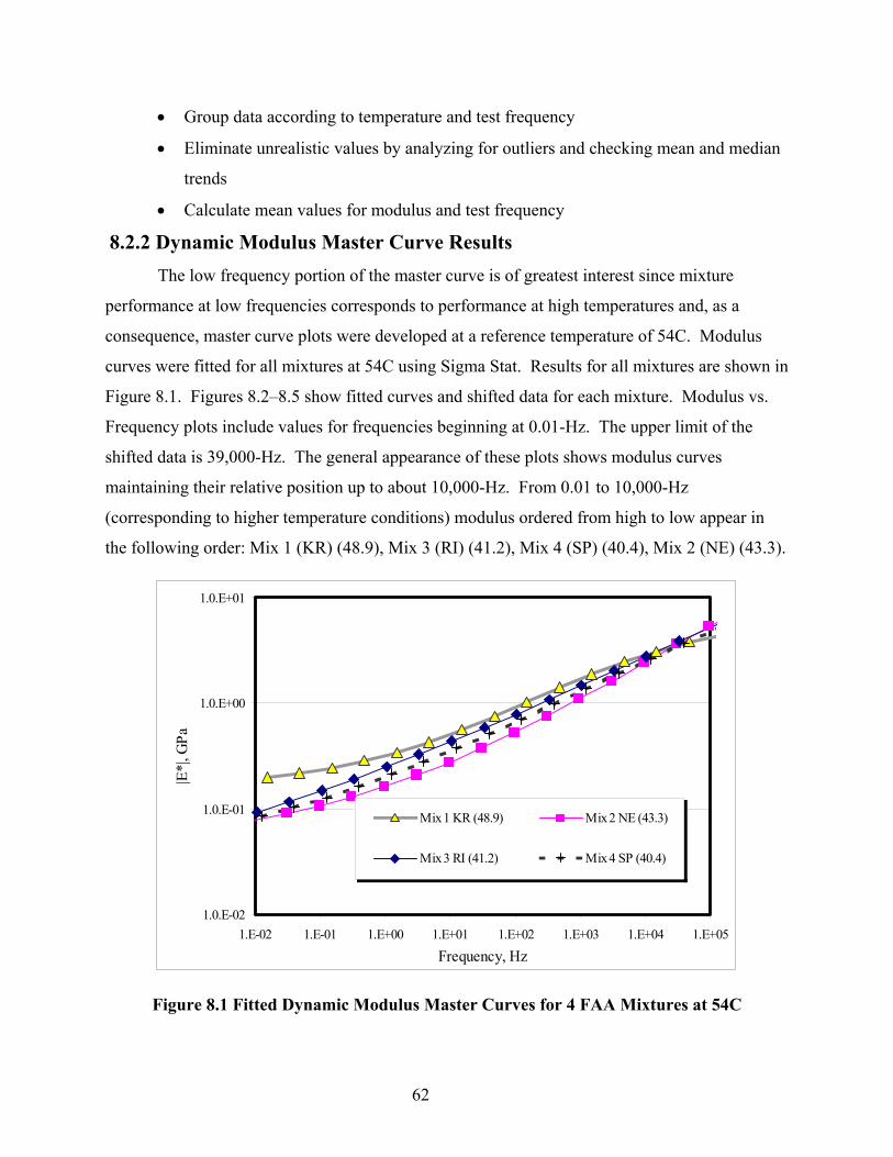
62
• Group data according to temperature and test frequency
• Eliminate unrealistic values by analyzing for outliers and checking mean and median
trends
• Calculate mean values for modulus and test frequency
8.2.2 Dynamic Modulus Master Curve Results The low frequency portion of the master curve is of greatest interest since mixture
performance at low frequencies corresponds to performance at high temperatures and, as a
consequence, master curve plots were developed at a reference temperature of 54C. Modulus
curves were fitted for all mixtures at 54C using Sigma Stat. Results for all mixtures are shown in
Figure 8.1. Figures 8.2–8.5 show fitted curves and shifted data for each mixture. Modulus vs.
Frequency plots include values for frequencies beginning at 0.01-Hz. The upper limit of the
shifted data is 39,000-Hz. The general appearance of these plots shows modulus curves
maintaining their relative position up to about 10,000-Hz. From 0.01 to 10,000-Hz
(corresponding to higher temperature conditions) modulus ordered from high to low appear in
the following order: Mix 1 (KR) (48.9), Mix 3 (RI) (41.2), Mix 4 (SP) (40.4), Mix 2 (NE) (43.3).
1.0.E-02
1.0.E-01
1.0.E+00
1.0.E+01
1.E-02 1.E-01 1.E+00 1.E+01 1.E+02 1.E+03 1.E+04 1.E+05
Frequency, Hz
|E*|
, GPa
Mix 1 KR (48.9) Mix 2 NE (43.3)
Mix 3 RI (41.2) Mix 4 SP (40.4)
Figure 8.1 Fitted Dynamic Modulus Master Curves for 4 FAA Mixtures at 54C

63
1.0.E-02
1.0.E-01
1.0.E+00
1.0.E+01
1.E-02 1.E+00 1.E+02 1.E+04 1.E+06 1.E+08 1.E+10 1.E+12
Frequency, Hz
|E*|,
GPa 20°C
40°C
54°C
Mix 1 (KR) Fit
Figure 8.2 Mix 1 (KR) Fitted |E*| Curve and Shifted Data at 54C
1.0.E-02
1.0.E-01
1.0.E+00
1.0.E+01
1.0.E+02
1.E-03 1.E-01 1.E+01 1.E+03 1.E+05 1.E+07 1.E+09 1.E+11
Frequency, Hz
|E*|
, GPa
20°C
40°C
54°C
Mix 2 Fit
Figure 8.3 Mix 2 (NE) Fitted |E*| Curve and Shifted Data at 54C

64
1.0.E-02
1.0.E-01
1.0.E+00
1.0.E+01
1.0.E+02
1.E-02 1.E+00 1.E+02 1.E+04 1.E+06 1.E+08 1.E+10 1.E+12
Frequency, Hz
|E*|
, GPa
20°C
40°C
54°C
Mix 4 Fit
Figure 8.4 Mix 3 (RI) Fitted |E*| Curve and Shifted Data at 54C
1.0.E-02
1.0.E-01
1.0.E+00
1.0.E+01
1.0.E+02
1.E-02 1.E+00 1.E+02 1.E+04 1.E+06 1.E+08 1.E+10 1.E+12
Frequency, Hz
|E*|
, GPa
20°C
40°C
54°C
Mix 4 Fit
Figure 8.5 Mix 4 (SP) Fitted |E*| Curve and Shifted Data at 54C
Figure 8.6 shows a plot of |E*| fitted/measured values. The plot shows some scatter from
0.8 to 1.2. Several greater values occur at 0.1-Hz in Mixtures 3 and 4.

65
0.6
0.8
1.0
1.2
1.4
1.E-02 1.E-01 1.E+00 1.E+01 1.E+02 1.E+03 1.E+04 1.E+05
Frequency, Hz
Fitte
d |E
*| /
Mea
sure
d |E
*|
Mix 1 KR Mix 2 NE Mix 3 RI Mix 4 SP
Figure 8.6 |E*| Fitted/Measured Values at 54C for the 4 Mixtures Investigated
The preceding plot of fitted-to-measured ratios shows that ratios decrease with increased
frequency. The larger fitted-to-measured ratios occur because greater levels of technical
difficulty are commonly encountered when gathering low-frequency, high-temperature dynamic
modulus data. This is true because of the resolution limitations of the testing equipment.
The following plots of |E*| ratios in Figures 8.7–8.10 show that at low temperature and
high frequency the high-FAA mixture (Mix 1) performs better that the other mixtures.

66
0
0.5
1
1.5
2
2.5
3
Increasing Frequency, Hz at 54C
|E*|
/|E*| MIX1/MIX 3
MIX1/MIX 4MIX 1/MIX 2
Figure 8.7 Performance Ratios for Mix 1
0
2
4
6
8
10
12
Increasing Frequency, Hz at 54C
|E*|
/|E*| MIX 2/MIX 1
MIX 2/MIX 3MIX 2/MIX 4
Figure 8.8 Performance Ratios for Mix 2

67
0
2
4
6
8
10
12
14
16
Increasing Frequency, Hz at 54C
|E*|
/|E*| MIX 3/MIX 1
MIX 3/MIX 4MIX 3/MIX 2
Figure 8.9 Performance Ratios for Mix 3
0
1
2
3
4
5
6
7
8
Increasing Frequency, Hz at 54C
|E*|
/|E*| MIX 4/MIX 1
MIX 4/MIX 3MIX 4/MIX 2t
Figure 8.10 Performance Ratios for Mix 4
8.3 Asphalt Pavement Analyzer Rut Susceptibility
APA testing results were described and presented in Chapter 7. Results and rankings are
given in Table 8.1 and Figure 8.11. Blend FAA is given in parenthesis in Figure 8.11. Table 8.1
shows rut depths obtained from averaging the results from two specimens per mixture and ranks

68
the mixtures according to performance at 8000 cycles. Figure 8.11 shows mixture rut
development per test cycle. Note the similarities in Mix 2 and Mix 3.
Table 8.1 Asphalt Pavement Analyzer Test Results (rut depth in mm).
Mix 1 (KR) Mix 2 (NE) Mix 3 (RI) Mix 4 (SP) 1 Cycle 0.906965 -0.41532 -0.14741 0.36382
5000 Cycles 4.513769 7.091806 7.11396 11.60078 8000 Cycles 4.566852 8.373692 8.42322 --
Mixture FAA 48.9 43.3 41.2 40.4 APA Rank at 8000 Cycles 1 3 2 4
0
2
4
6
8
10
12
0 1000 2000 3000 4000 5000 6000 7000 8000
Cycles
Rut
Dep
th [m
m]
KR (48.9) NE (43.3) R (41.2) SP (40.4)
Figure 8.11 APA Rutting Curves at 54C
8.4 Mixture FAA Flow Time The method of least squares shows that the flow time of a standard FAA sample through
the FAA test apparatus is strongly related to FAA. According to the Chapter 4 experimental
results, R2 = 0.91 for the equation: TIME (FAA) = 0.1556(FAA)–1.5098. Using this result,
measured blend FAA’s, standard error of the prediction, and t-distribution critical values, FAA
flow time may be estimated for mixture blends 1–4. Table 8.2 shows standard error of the

69
prediction, and 95% confidence intervals for (n–2) = 9 degrees of freedom. Figure 8.12 shows
predicted vs. measured timing values. The prediction for Mix 1 is an extrapolated value.
Table 8.1 FAA Flow Timing Prediction (95% CI, 9 df)
FAA prediction (sec) SE prediction t * SE prediction Meas Time Mi
x 1 KR
48.9 6.59 0.231 0.52 6.43
Mix 2 NE 43.3 5.66 0.224 0.51 5.73 Mix 3 RI 41.2 5.31 0.221 0.50 5.21 Mix 4 SP 40.4 5.18 0.220 0.50 5.19
5
5.5
6
6.5
7
5 5.5 6 6.5 7
Predicted FAA Timing, sec
Mea
sure
d FA
A Ti
min
g, se
c
FAA MixtureBlends
Figure 8.12 Blend FAA, Measured vs. Predicted FAA Timing
8.5 Analysis of Experimental Data Analysis is presented in three parts. Part one discusses and analyzes APA data with
respect to rate of rutting. Part two ranks mixtures in terms of performance according to the effect

70
of FAA, aggregate type, and manufacture method. Part three correlates APA Rut Depth and all
variables discussed in this study.
8.5.1 APA Data Analysis
Data is collected for each APA loading cycle. It is therefore possible to analyze the APA
Rut Test data shown in Figure 8.11 for rate of rutting. Table 8.3 and the associated plot in Figure
8.13 describe trends in rut depth along various portions of the APA rutting curve.
Table 8.2 APA Rutting Rate, Test Temperature 54C
Mix 1 (KR)
Mix 2 (NE)
Mix 3 (RI)
Mix 4 (SP)
Rutting Rate [mm/Cycle] Max Rutting Rate Value 0.0110 0.0054 0.0053 0.0244
0 – 500 Cycles 0.0034 0.0041 0.0045 0.0114 500 – 1000 Cycles 0.0009 0.0028 0.0032 0.0032
1000 – 2000 Cycles 0.0013 0.0014 0.0014 0.0016 2000 – 3000 Cycles 0.0005 0.0009 0.0009 0.0012 3000 – 5000 Cycles 0.0002 0.0007 0.0007 0.0009 5000 – 7000 Cycles 0.0001 0.0004 0.0005 NA
Mean Slope
7000 – 8000 Cycles 0.0002 0.0004 0.0004 NA Max Difference Between
Concurrent Rutting Rate Values 0.0040 0.0035 0.0016 0.0019
Table 8.3 shows averages of the highest-FAA mixture rutting are approximately one
quarter the rate of the lowest-FAA mix. Note that the high-angularity mixture exhibits both the
lowest rate of rutting throughout the test and the maximum difference in concurrent rate values.
This difference is an indicator of the noise present in the rutting rate plot. Both high angularity
mixtures have the more noise, especially after 4000 APA test cycles. It may be speculated that
the noise in the rutting rate curve is present due to rearrangement of the aggregates.

71
-0.0025
0.0025
0.0075
0.0125
0.0175
0.0225
0 1000 2000 3000 4000 5000 6000 7000 8000
Cycles
Delt
a Ru
t Dep
th [m
m/c
ycle] KR (48.9)
NE (43.3)RI (41.2)
SP (40.4)
Figure 8.13 APA Rutting Rate per Test Cycle, Temperature 54C
.
8.5.2 Performance Ranking Tables 8.4–8.6 give performance rankings in terms of effect of FAA, aggregate type, and
manufacture method.
Test results suggest that at high temperatures the effect of FAA will be as presented in
Table 8.4. Based on least squares analysis of test results, there appears to be a slight performance
benefit from increasing mixture FAA. Recall that Superpave FAA criterion is 40<FAA<45. The
FAA value of Mixture 2 (43.3) nears the upper end of this criterion. The plot of Modulus vs.
FAA in Figure 8.14 shows the variation in average |E*| explained by FAA correlates at R2 = 0.85
for a |E*|[GPa] = 0.0138 (FAA)–0.4876. The plot of APA Rut Depth vs. FAA in Figure 8.15
shows a best-fit line correlates at R2 = 0.91 for APA [mm] = 0.7922 (FAA)+42.486.

72
Table 8.3 FAA and Related High Temperature (54C) Mix Performance Ranking
Mixture Mixture FAA Rank
Mixture APA Rutting Performance Rank
Modulus Master Curve Performance Rank
Mix 1 KR 1 1 1 Mix 2 NE 2 3 4 Mix 3 RI 3 2 2 Mix 4 SP 4 4 3
y = 0.0138x - 0.4876R2 = 0.8513
0
0.05
0.1
0.15
0.2
0.25
40 42 44 46 48 50
Mixture FAA
|E*|
, GPa
|E*| [Gpa] vs. FAA Linear (|E*| [Gpa] vs. FAA)
Figure 8.14 |E*| vs. FAA at 0.01 Hz and Test Temperature 54C

73
y = -0.7922x + 42.486R2 = 0.9149
0
2
4
6
8
10
12
14
40 42 44 46 48 50
Mixture FAA
APA
Rut
Dep
th, m
m
APA Depth [mm] vs. FAA Linear (APA Depth [mm] vs. FAA)
Figure 8.15 APA Rut Depth vs. FAA
The effect of aggregate type is presented in Table 8.5. Even though the Mixture 2
aggregate blend included diverse materials and a satisfactory gradation the modulus performance
was low, especially when compared to the Mixture 1 blend that was composed of similar
materials. This suggests poor interaction between blend components for Mix 2.
Table 8.4 Aggregate Related High Temperature (54C) Mixture Performance
Mixture Aggregate Type Mixture APA Rutting Performance Rank
Modulus Master Curve Performance Rank
Mix 1 KR Limestone – Limestone 1 1
Mix 2 NE Gravel – Granite – Limestone 3 4
Mix 3 RI Gravel – Limestone 2 2 Mix 4 SP Gravel – Limestone 4 3
Table 8.6 presents the effect of including crushed material in the mixture blend. Even
though Mixture 2 material included crushed coarse aggregate and manufactured sand its modulus
performance was low when compared with mixtures having less crushed material. As in
aggregate related performance, this suggests poor interaction between blend components.

74
Table 8.5 Crushing Related High Temperature (54 C) Mixture Performance
Mixture Manufactured Material in Blend
Mixture APA Rutting Performance Rank
Modulus Master Curve Performance Rank
1 100% 1 1 2 50% 3 4 3 30% 2 2 4 30% 4 3
8.5.3 Performance – Mixture Characteristics Correlation Several kinds of mixture characteristics were examined in this project. In order to
identify characteristics related to mixture performance it is important to have a method of sorting
and relating mixture parameters and performance related mechanical properties. In this section
Pearson correlation coefficients are used to identify characteristics that explain performance.
Table 8.7 shows Pearson correlation coefficients for APA Rut Depth and all variables
discussed in this study. Values near 1 show strong positive correlation and those near –1 show
strong negative correlation. Variables include: dynamic modulus at 54C and 0.01-Hz, FAA,
Min., Max., Median, and quartile values obtained for blended AIMS data (reference Chapter 6),
and mixture blend measured FAA Flow Timings. The table shows that rut depth is highly
correlated with several variables, most notably |E*|, FAA, and Maximum Radial Angularity.
Correlation results suggest that rutting performance is strongly related to the following six
characteristics:
• modulus (0.01-Hz at 54C)
• FAA
• FAA Flow Time
• Radian Angularity (Minimum, 1st Quartile and Maximum)
• Gradient Angularity (Minimum and 1st Quartile)
• Form, 2-D (Minimum and 1st Quartile)
Additionally, strong relationships were observed for modulus and:
• FAA
• Gradient Angularity (Minimum), and
• FAA Flow Time.

75
Table 8.6 Pearson Correlation for FAA Statistics (23)
Rut Depth
|E*| at 0.01Hz FAA Rad
Min Rad Q1 Rad Med Rad Q3 Rad
Max |E*| at 0.01Hz -0.926
FAA -0.957 0.923
Rad Min -0.820 0.632 0.879 Rad Q1 -0.875 0.665 0.879 0.982 Rad Median -0.602 0.321 0.651 0.934 0.913 Rad Q3 -0.585 0.312 0.647 0.933 0.903 0.999 Rad Max -0.946 0.957 0.993 0.817 0.816 0.556 0.554 Grad Min -0.923 0.999 0.935 0.654 0.677 0.344 0.338 0.968Grad Q1 -0.846 0.730 0.937 0.979 0.945 0.853 0.857 0.895Grad Median -0.663 0.491 0.788 0.966 0.902 0.938 0.948 0.722Grad Q3 0.029 -0.126 0.212 0.512 0.357 0.626 0.661 0.151Grad Max -0.721 0.680 0.883 0.900 0.819 0.756 0.772 0.858Form Min -0.894 0.808 0.972 0.957 0.932 0.792 0.794 0.943Form Q1 -0.836 0.640 0.880 0.999 0.990 0.933 0.929 0.817Form Median -0.768 0.580 0.848 0.996 0.963 0.947 0.949 0.783Form Q3 -0.419 0.098 0.458 0.826 0.804 0.973 0.972 0.350Form Max -0.721 0.492 0.785 0.986 0.960 0.980 0.980 0.707
FAA Time -0.911 0.865 0.989 0.918 0.895 0.716 0.719 0.973
Grad Min
Grad Q1
Grad Med
Grad Q3
Grad Max
Form Min
Form Q1
Form Med
Form Q3
Form Max
Grad Q1 0.755
Grad Median 0.525 0.954 Grad Q3 -0.074 0.509 0.716 Grad Max 0.716 0.961 0.933 0.638 Form Min 0.830 0.992 0.910 0.416 0.950 Form Q1 0.660 0.973 0.953 0.474 0.881 0.953 Form Median 0.606 0.975 0.985 0.588 0.914 0.944 0.991 Form Q3 0.120 0.712 0.854 0.657 0.610 0.630 0.825 0.849 Form Max 0.516 0.940 0.976 0.596 0.858 0.897 0.983 0.992 0.908
FAA Time 0.884 0.973 0.862 0.353 0.941 0.993 0.913 0.900 0.537 0.841
Plots of FAA explaining the previously mentioned relationships are presented in Figures 8.11,
8.12, and 8.16 - 8.18.

76
y = 0.7179x - 17.551R2 = 0.9855
y = 0.0314x + 1.7999R2 = 0.7718
y = 0.0917x + 1.4907R2 = 0.773
0
2
4
6
8
10
12
14
16
18
40 41 42 43 44 45 46 47 48 49 50
Mixture FAA
Rad
ian
Ang
ular
ity
Radian Ang (min) vs. FAA Radian Ang (Q1) vs. FAARadian Ang (max) vs. FAA Linear (Radian Ang (max) vs. FAA)Linear (Radian Ang (min) vs. FAA) Linear (Radian Ang (Q1) vs. FAA)
Figure 8.16 Blend Radian Angularity vs. FAA
y = 0.1353x + 0.1866R2 = 0.7746
y = 0.1206x - 1.6878
2
3
4
5
6
7
8
40 41 42 43 44 45 46 47 48 49 50
Mixture FAA
2D F
orm
Inde
x
2D Form (min) vs. FAA 2D Form (Q1) vs. FAALinear (2D Form (Q1) vs. FAA) Linear (2D Form (min) vs. FAA)
Figure 8.17 Blend Form Index vs. Blend FAA

77
GradQ1 = 80.421x - 1067.2R2 = 0.877
GradMin = 130.02x - 4816.5R2 = 0.8746
0
500
1000
1500
2000
2500
3000
40 41 42 43 44 45 46 47 48 49 50
Mixture FAA
Gra
dien
t Ang
ular
ity
Gradient Ang (min) vs. FAA Gradient Ang (Q1) vs. FAALinear (Gradient Ang (Q1) vs. FAA) Linear (Gradient Ang (min) vs. FAA)
Figure 8.18 Blend Gradient Angularity vs. FAA.
The plot of APA rut depth in Figure 8.11 shows a negative dependence upon FAA. The
regression of APA on FAA was fitted according to the following:
APA(mix FAA) [mm] = -0.7922(mix FAA)+42.486
R2 = 0.9149
Dynamic modulus was fitted according to the following linear trend in Figure 8.11:
|E*|(mix FAA) [GPa] = 0.0138(mix FAA) - 0.4876
R2 = 0.8513
This relationship holds for test temperature 54C.
Linear regression results show that for this testing scenario, APA rut depth and dynamic
modulus were well represented by mixture FAA. However, notice that the variation in modulus
is small (the coefficient is 0.0138) with respect to change in FAA. This suggests that blend FAA
does not greatly influence modulus at high temperatures. The FAA coefficient in the APA rut
depth regression equation is –0.79, which implies that rutting resistance is strongly influenced by
the blend FAA magnitude.
78
A number of characteristics exhibited strong correlation with FAA, but also exhibited
lower levels of influence when compared to APA rutting. They are listed below and are
recommended for additional evaluation in future research.
Results from the FAA flow time test correlate well with modulus, APA and FAA. The
test is attractive since it is easily performed. It is recommended that additional evaluation should
be conducted on flow time and performance.
Radian Angularity (Minimum, 1st Quartile and Maximum), Gradient Angularity
(Minimum and 1st Quartile), and 2-D Form (Minimum and 1st Quartile) correlate well with APA
and FAA. These characteristics are recommended for inclusion in future research.
8.6 Conclusions The purpose of Chapter 8 was to present an analysis of testing results for FAA validation.
The testing program included several means of evaluating aggregate materials and asphalt
mixtures. Four mixtures were designed and evaluated.
In previous tasks, aggregate materials were classified according to aggregate type,
manufacture method, flow timing, and FAA. FAA Flow Timing descriptions were established
for aggregates and aggregate blends using statistical predictions.
Superpave FAA criteria requires that aggregate materials are evaluated according to
AASHTO T304 (Method A) for measurement of the uncompacted void content of fine
aggregate. Digital imaging angularity and form measurements were also included for
comparison with AASHTO T304.
A dynamic modulus testing program was used to evaluate the asphalt mixtures. Master
curves were developed at reference temperature 54C and were obtained by inputting modulus,
test frequency, and test temperature information into statistical software for nonlinear regression
analysis. Regression analysis included fitting data to a sigmoidal function that has been shown
to represent asphalt mixture behavior. Values from the sigmoidal master curve models were
used for analysis.
Additional mixture evaluation was also performed for rutting resistance using an APA
rut-testing machine, also at test temperature 54C. The analysis included ranking performance
based on rut depth and modulus magnitude according to aggregate type and manufacture method.
It was observed that:

79
• Composite aggregate blends having similar components exhibited better modulus and rutting
performance,
• For these aggregate materials, the inclusion of manufactured (crushed) materials did not
proportionally affect modulus or rutting performance, as shown in Table 8.6. The high-FAA
mixture exhibited high modulus values and high rutting resistance but modulus and rutting
did not strongly depend on FAA for mixtures having FAA below approximately 43.3.
A correlation matrix for all the material parameters measured or calculated in this study
was developed using statistical software. The results shown in table 8.7 indicate that the APA
rut measurements have the highest correlation with FAA (R2 = 91.6%). For the |E*| measured at
54C and 0.01-Hz the highest correlation was obtained with Grad Min (R2 = 99.8%), with the
FAA following in third place (R2 = 85.2%).

80
CHAPTER 9: SUMMARY AND CONCLUSIONS Summary
In Chapter 2 the use of standard FAA testing was described with regard to historical
implementation and post-Superpave research in research papers and nationally accepted texts.
Chapter 2 also reviewed descriptions of new trends in characterizing aggregate angularity
through digital imaging techniques. Traditional concepts have indicated that HMA aggregates
should be angular and have a rough texture. It was found in post-Superpave research that high
angularity by standard FAA did not always result in better rutting performance. Additionally, it
was found through imaging techniques that crushing increases angularity but may not produce
aggregate having rough texture.
A breakdown of standard FAA values obtained by Mn/DOT was given in Chapter 3. A
total of 3,976 Mn/DOT standard FAA values were obtained using the State of Minnesota
Database (LIMS) and Metro District production records. These records spanned the time period
2000–2002. This data set included 1,268 Superpave mixture designs, and was reduced to 980
values by setting the requirement for “useable” data as points having both a bit-record number
and a project number description.
The reduced data set was sorted using project number and bitrecord. FAA values from
the sorted data were then averaged. 59 averaged values were obtained. It was also possible to
sort the 59 averaged values according to Mn/DOT bituminous mixture type. Four mixtures types
were present, including Mn/DOT 2360 Superpave mixtures SPWEB340, SPWEB440, and
SPWEB540. Mixture data was also available for MVWE35035.
Plots of averaged FAA data showed a gap in average FAA data between mixture type
SPWEB340 and SPWEB440. Additionally, frequency increases for FAA values ranging from
40–41 and 44.4–45. Additionally, the plot shows a trend in decreasing frequency of FAA values
between 41 and 44.4.
Mixture proportion data was obtainable from the LIMS database, and was later used as a
reference to evaluate mixture designs produced by the project staff.

81
In Chapter 4 standard FAA data was obtained and analyzed for 11 Minnesota aggregates
using AASHTO T304 Method A. Two simple experiments were also included to further
examine the results of AASHTO T304. Experiment 1 included varying the testing apparatus
drop height. It was observed that FAA values for a given aggregate material varied somewhat
with drop distance. However, the order of FAA measurements between materials was
maintained regardless of drop distance. Experiment 2 included measurement of the aggregate
flow time through the FAA test funnel. A strong relation was found between FAA and flow
time.
Digital Aggregate Imaging System (AIMS) characterization was included for 8 of the
aggregates. Analysis was conducted by the Texas A&M Department of Civil Engineering. Fine
aggregate imaging results included 2-dimensional form, gradient angularity, and radial
angularity.
Chapter 5 outlined the development of a laboratory testing program for FAA validation.
The program included both aggregate and mixture testing. The aggregate testing included
gradation analysis, specific gravity and absorption, as well as standard FAA testing. Mixture
tests included dynamic modulus (|E*|) and asphalt pavement analyzer (APA) rut testing. In order
to minimize variables, |E*| and APA specimens would be designed according to Mn/DOT 2360
Superpave volumetric and traffic design criteria. The test specimens should all have similar air
voids, VMA, VFA, and asphalt binder. The effect of FAA will be investigated by having 2 high-
FAA mixtures and 2 low-FAA mixtures.
Asphalt mixture formulation was described in Chapter 6. Four laboratory mixture
designs were produced using 2 high-FAA and 2 low-FAA aggregate blends. Mixture design was
performed according to the guidelines from Mn/DOT Specification 2360. 4800-g trial mixture
specimens were produced and subsequently evaluated using ASTM D 2041and ASTM D 2726.
Aggregate blends were evaluated for angularity using both measured and estimated FAA
calculations. The best method of estimation was observed to be a gradation-weighted average.
It is important to note that the FAA estimates are for four similar blends, having 20-30% of a
single coarse material. Averaging should be used carefully when estimating the FAA of other
blends. It is best to know the contribution of coarse material to FAA.

82
Digital imaging angularities were also calculated for each blend based upon
measurements obtained for individual component aggregates. Median and quartile values were
used to describe the blend imaging angularities.
Chapter 7 describes specimen fabrication and testing for FAA validation purposes. For
each mixture, four 100 by 150-mm specimens were produced for |E*| testing as well as two
additional 150 by 75-mm specimens for APA testing. Specimens were fabricated to Mn/DOT
Specification 2360 criteria and specimen air voids were targeted at 5%.
Raw modulus data was analyzed using the SINAAT complex modulus spreadsheet for
asphalt concrete. The final set of modulus values depended on statistical and graphical
evaluation of potential outlying data points. Outlier evaluation included comparisons of
individual data points with 1.5 by (inter-quartile range) and also plotted trends in mean and
median. Using dynamic modulus data, master curves were developed at reference temperature
54C and were obtained by inputting modulus, test frequency, and test temperature information
into statistical software for nonlinear regression analysis. Regression analysis included fitting
data to a sigmoidal function that has been shown to represent asphalt mixture behavior. Values
from the sigmoidal master curve models were used for analysis.
APA testing data was acquired for the four mixtures using an 8000-cycle test at
temperature 54C. Results were reported as average rut depth.
Conclusions A correlation matrix for all the material parameters measured or calculated in this study
was developed using statistical software. The results shown in chapter 8 in table 8.7 indicate that
the APA rut measurements have the highest correlation with FAA (R2 = 91.6%). Correlation
results show strong relationships between rut resistance and several other characteristics,
including digital imaging characterization measurements of Gradient Angularity, Radian
Angularity, and Form Index.
For the |E*| measured at 54C and 0.01-Hz the highest correlation was obtained with Grad
Min (R2 = 99.8%), with the FAA following in third place (R2 = 85.2%).
The results obtained in this study indicate that the current FAA specification does a
reasonable job in selecting the fine aggregates for asphalt mixtures with enhanced rut resistance.
High correlations were found between FAA and APA rut depths and FAA and |E*| at 0.01-Hz,

83
both measured at 54C. However, the visual inspection of linear trends (Figures 8.14, 8.15)
showed that FAA had little influence on modulus variation and rut depth for the mixtures with
FAA below approximately 43.3. This trend should be interpreted with caution as the results
presented were based on four laboratory-produced mixtures that contained only 2 or 3
component aggregates to minimize the factors in the analysis. Mixtures found in the field often
have as many as 5 or more components and tend to have more fine aggregates, which most likely
will increase the effect of FAA magnitude on mixture properties.
Future research should include evaluation of both contractor-produced and laboratory-
produced blends and mixtures taking into consideration additional issues such as film thickness
that is not part of the current MnDOT mix design. Note that the surface area for Mixtures 1–4
was calculated to be 23.3, 21.2, 26.1, and 20.8-ft2/lb, respectively, which according to recent
calculations performed by MnDOT Office of Materials at the conclusion of the project are low in
comparison to gradation blend surface areas normally observed in field mixes (around 28-ft2/lb).

84
References
1. Superpave Series No. 2 (SP-2). The Asphalt Institute, Lexington, KY, 1996. pp. 28–30.
2. Standard Specifications for Construction, Minnesota Department of Transportation, St. Paul,
MN, 2000.
3. Jahn, David W., Conference Presentation: Fine Aggregate Angularity. Superpave Expert
Task Group Conference, University of Minnesota, Minneapolis, MN, August 28, 2002.
4. Coree, Brian J. and Walter P Hislop, The Difficult Nature of VMA: A Historical Perspective,
November 1998, Transportation Research Board 78th Annual Meeting, 1999.
5. Roberts, Freddy L., Prithvi S. Kandhal, E. Ray Brown, Day-Yinn Lee, Thomas W. Kennedy,
Hot Mix Asphalt Materials, Mixture Design and Construction, 2nd Edition. NAPA Education
Foundation, Lanham, MD, 1996, pp. 147–148.
6. White, Thomas D. (Principal Investigator), Effect of Fine Aggregate Angularity on Asphalt
Mixture Performance. TRB subject code: 31-1 Bituminous Aggregate Bases. Publication
No: FHWA/IN/JTRP-98/20, SPR-2153. Final Report, July 1999.
7. Kandhal, Prithvi S., and F. Parker, Jr., Aggregate Tests Related to Asphalt Concrete
Performance in Pavements, NCHRP report 405, TRB, National Academy Press, Washington
D.C., 1998.
8. Button, Jow W., Dae-Wook Park, Arif Chowdhruy, Dallas Little, and Eyad Masad, Effects of
Fine Aggregate Properties on Rutting Resistance, International Society for Asphalt
Pavements Ninth International Conference On Asphalt Pavements, August 17 - 22, 2002.
Danish Road Directorate, Ministry of Transport, Denmark, Elisagaardsvej 5, Roskilde, 4000,
Denmark.
9. 2003.Fletcher, Thomas, Chandan Chandan, Eyad Masad, and Krishna Sivakumar, Aggregate
Imaging System (AIMS) for Characterizing the Shape of Fine and Coarse Aggregates,
Transportation Research Record. No.1832, pp. 67–77. Transportation Research Board,
Washington, D.C., 2003.
10. Al–Rousan, Taleb, Eyad Masad, Leslie Myers, Dallas Little and John D’Angelo, Aggregate
Shape Classification System Using AIMS. Federal Highway Administration, Washington,
D.C., Transportation Research Board 83rd Annual Meeting, January 11-15, 2004.

85
11. Kandhal, Prithvi S., Frazier Parker, Jr., and Rajib B. Mallick, Aggregate Tests for Hot-Mix
Asphalt: State of the Practice, Transportation Research Circular No. 479, December 1997.
12. National Center for Asphalt Technology, Asphalt Technology News, vol. 15, no. 2. National
Center for Asphalt Technology, 277 Technology Parkway, Auburn, Alabama 36830, Fall
2003.
13. Mn/DOT Lab Manual, Section 1206, Minnesota Department of Transportation, April 17,
2000.
14. AASHTO T84 (Mn/DOT Modified – Lab Manual section 1205), Minnesota Department of
Transportation, St. Paul, MN, October 2002.
15. AASHTO T85 (Mn/DOT Modified – Lab Manual section 1204), Minnesota Department of
Transportation, St. Paul, MN, May 2001.
16. Das, Braja M., Principles of Geotechnical Engineering, 4th edition. PWS Publishing, Boston,
MA 1998, pp. 40–41.
17. Vavrik, William R., William J. Pine, Gerald Huber, Samuel H. Carpenter, and Robert Bailey,
The Bailey Method of Gradation Evaluation: The Influence of Aggregate Gradation and
Packing Characteristics on Voids in the Mineral Aggregate, Journal of the Association of
Aspahlt Paving Technologists, vol. 70, 2001, pp. 132-175.
18. 2002 Design Guide Draft – 2.4 Modulus of Elasticity for Major Material Groups, NCHRP
Project 1-37A, 2002.
19. Advanced Asphalt Technologies, SINAAT: Spreadsheet for Analysis of Complex Modulus
Data on Asphalt Concrete Specimens, version 2.0. Advanced Asphalt Technologies, LLC,
State College, PA, July 9, 2001.
20. Moore, David S. and George P. McCabe, Introduction to the Practice of Statistics, 3rd
Edition. W. H. Freeman and Company, New York, NY 1999.
21. Sigma Stat for Windows version 1.0, Jandel Corporation, 1994.
22. Pellinen, T. K., and M. W. Witczak, “Stress Dependent Master Curve Construction for
Dynamic (Complex) Modulus,” Journal of the Association of Asphalt Paving Technologists,
vol. 71, 2002.
23. Statistix for Windows version 7.0. Analytical Software, 2000.

A-1
APPENDIX A The following table, as referenced in Chapter 3, presents a list of Mn/DOT LIMS data
from year 2000 – 2002. For this data set it is possible to cross-reference bitrecord, project
number and FAA.
Table A.1. 59 Mn/DOT Bit-Record and Project Numbers with FAA
P_BIT REC Samples/P_BIT REC P_MIX P_PROJ NO AVG FAA 000019 27 4001-44 40.6 000056 12 4603-38 44.0 000079 12 5203-84 42.4 000101 19 1480-127 43.6
0-2001-133 17 2785-316 45.1 0-2001-170 10 1901-137 44.8 0-2001-210 32 7007-24 45.8 0-2001-275 11 SPNWC430 0208-102 45.5 0-2001-477 18 SPWEB440 2758-60 46.4 0-2002-026 12 SPWEB540 6284-131 45.7 0-2002-042 10 SPWEB440 1913-56 44.8 0-2002-165 10 SPWEB440 6221-40 45.7 0-2002-224 14 SPNWC430 1004-24 44.7 0-2002-246 13 SPWEB440 1004-24 43.9 04-2001-033 24 5606-40 43.2 04-2002-018 22 MVWE35035 1414-02 42.7 04-2002-052 14 MVWE35035 7805-31 42.6 06-2002-148 10 SPNWB430 7408-29 45.2 07-2001-010 13 6704-16 41.8 07-2001-017 18 3206-17 41.2 07-2001-044 12 0804-72 41.3 07-2001-076 30 2280-119 46.2 07-2001-077 24 0704-78 41.1 07-2001-102 18 4001-45 41.2 07-2002-012 13 SPWEB440 7205-21 46.8 07-2002-022 16 SPWEB440 5380-112 45.4 07-2002-048 15 SPWEB340 1703-64 42.9 07-2002-055 12 MVWE35035 165-999-01 42.5 07-2002-072 11 SPWEB340 5905-21 42.5
2000-077 17 1905-24 43.7 2000-108 12 2735-160 41.4 2000-119 10 1013-70 45.5 2000-231 12 8209-41 42.5 2000-304 23 1301-87 44.9 2001-007 15 1209-20 40.8

A-2
2001-007 12 1210-09 40.5 2001-041 16 6402-20 41.1 2001-054 19 6402-20 40.9 2001-077 13 3703-21 41.3
2001-127 15 spweb540 2785-316 45.8 2001-133 47 spweb540 2785-316 45.4 2001-210 34 spweb540 7007-24 45.8 2001-329 10 spnwb440 1921-67 47.3 2002-042 13 SPNWB330 4105-08 40.8 2002-047 17 SPWEB340 4105-08 41.9 3-2000049 12 1809-49 41.5 3-2000051 27 7380-205 46.5 3-2000121 20 0116-44 41.9 3-2000143 10 1804-48 41.9 3-2000170 14 1810-82 41.3
3A-2001-049 28 8606-50 40.7 3A-2001-064 10 1814-01 40.6 3A-2001-122 27 3302-12 40.0 3A-2002-079 10 SPWEB440 1115-18 44.7 3A-2002-096 13 SPWEB340 8604-30 43.2 3A-2002-142 14 SPWEB340 7319-34 44.5 3A-2002-146 11 MVWE35035 1809-58 41.5 3A-2002-150 10 SPWEB440 1115-18 45.3 8A-2001-011 20 3411-63 40.7