Validation of Scaffold Design Optimization in Bone Tissue ... · PDF fileValidation of...

Validation of Scaffold Design Optimization in Bone

Tissue Engineering: Finite Element Modeling versus

Designed Experiments

Nicholas Uth1, Jens Mueller2, Byran Smucker3, Azizeh-Mitra Yousefi1*

1Department of Chemical, Paper and Biomedical Engineering, Miami University, Oxford,

OH 45056, USA

2Research Computing Support, Miami University, Oxford, OH 45056, USA

3Department of Statistics, Miami University, Oxford, OH 45056, USA

*Corresponding author: Azizeh-Mitra (Amy) Yousefi; [email protected]; (513) 529-0766

mailto:[email protected]

Abstract

This study reports the development of biological/synthetic scaffolds for bone tissue engineering via

3D bioplotting. These scaffolds were composed of poly(L-lactic-co-glycolic acid) (PLGA), type I

collagen, and nano-hydroxyapatite (nHA) in an attempt to mimic the extracellular matrix of bone. The

solvent used for processing the scaffolds was 1,1,1,3,3,3-Hexafluoro-2-propanol (HFP). The produced

scaffolds were characterized by scanning electron microscopy, microcomputed tomography,

thermogravimetric analysis, and unconfined compression test. This study also sought to validate the

use of finite-element optimization in COMSOL Multiphysics for scaffold design. Scaffold topology

was simplified to three factors: nHA content, strand diameter, and strand spacing. These factors affect

the ability of the scaffold to bear mechanical loads and how porous the structure can be. Twenty four

scaffolds were constructed according to an I-optimal, split-plot designed experiment (DE) in order to

generate experimental models of the factor-response relationships. Within the design region, the DE

and COMSOL models agreed in their recommended optimal nHA (30%) and strand diameter (460

µm). However, the two methods disagreed by more than 20% in strand spacing (923 µm for DE; 601

µm for COMSOL). Seven scaffolds were 3D-bioplotted to validate the predictions of DE and

COMSOL models (4.5 - 9.9 MPa measured moduli). The predictions for these scaffolds showed

relative agreement for scaffold porosity (mean absolute percentage error of 4% for DE and 13% for

COMSOL), but were substantially poorer for scaffold modulus (52% for DE; 21% for COMSOL),

partly due to some simplifying assumptions made by the models. Expanding the design region in future

experiments (e.g., higher nHA content and strand diameter), developing an efficient solvent

evaporation method, and exerting a greater control over layer overlap could allow developing PLGA-

nHA-collagen scaffolds to meet the mechanical requirements for bone tissue engineering.

Keywords: bone tissue engineering, optimization, simulation, additive manufacturing, 3D bioplotting,

designed experiment, scaffold topology, COMSOL

1 Introduction

Bone tissue has a limited capacity for regeneration depending on the extent of the damage and the

bone involved [1]. In order to repair critical-size defects and nonunions, either bone grafts or

synthetic bone-graft substitutes are used to replace the tissue [2]. Grafts and substitutes are in such

common use that, every year, at least four million operations worldwide make use of them [3], and

this number will only increase as global populations grow. However, there are risks and limitations

to these treatments. Bone-graft substitutes are subject to wear over time, immune response, or bone

thinning due to stress shielding [2,3]. Grafts taken from donors (allografts) risk immune response

or disease transmission [2,3], and grafts from the patient (autografts), while considered ideal, are

limited in size/quantity and risk donor site complications and infection [2,3]. Bone tissue

engineering (TE) aims to enable the patient’s body to regenerate the damaged tissue without the

need for a donor or risk of spurring immunological action [4–6].

In order to regenerate damaged tissues, TE makes use of porous scaffolds made of

biomaterials to act as a cellular matrix and support structure [6–8]. In designing scaffolds, the

general consensus is that they should behave as similarly to the tissues they are meant to replace

as possible [9,10]. In the case of bone tissue, it is hypothesized that scaffolds need to have a high

modulus and adequate porosity based on the bone to be replaced (Table 1), as mechanoregulatory

effects are believed to be the key factor in bone tissue regrowth and cellular differentiation

[8,9,11,12]. If the scaffold environment (mechanical forces transferred to the cells and

vascularization) is unlike physiological conditions, there is a risk that mesenchymal stem cells

(MSCs) will differentiate into chondrocytes or fibroblasts, which grow cartilage and fibrous tissues

respectively [13,14]. However, stiffness and porosity directly conflict as design factors, which

makes the design process critical [15].

Table 1. Mechanical properties of mature bone tissues, as described by literature.

Young’s

Modulus

50 - 100 MPa (Trabecular bone) [16]

2.23 - 25.9 GPa (Trabecular bone) [17]

20 GPa [18]

6 GPa [19]

1.3 - 20 GPa (Trabecular bone) [20]

Porosity

< 15 % (Cortical bone) [21]

> 70 % (Trabecular bone) [21]

50 - 90 % (Trabecular bone) [22]

There are two key aspects to scaffold design: material choice and topology, both of which

can be adjusted to produce scaffolds with properties akin to native tissue [21]. The material choices

affect how readily the scaffold will biodegrade, and whether the scaffold will be bioactive [22].

While each class of biomaterial (polymers, metals, and ceramics) have their own individual

disadvantages that can restrict their applications in TE, composites can mitigate these limitations

and it has been suggested that they can exhibit tissue-mimicking properties [4]. This study made

use of a polymer-ceramic-protein composite, which combined the ease of use and controlled

biodegradation rate of poly(L-lactic-co-glycolic acid) (PLGA), the mechanical strength and

bioactivity of nano-hydroxyapatite (nHA), and the cellular adhesiveness of collagen.

PLGA is a synthetic random copolymer of poly(L-lactic acid) (PLLA) and polyglycolic

acid (PGA), and has U.S. Food and Drug Administration (FDA) approval for some use in humans

[4]. Its degradation rate has been shown to be customizable in the range of weeks to months based

on the ratio of PLLA to PGA. However, PLGA has a low modulus even compared to its component

polymers (PLGA 85:15 E = 2.0 GPa, PLLA E = 2.7 GPa, PGA E = 7.0 GPa [23]) due to its

amorphous structure. Therefore, on its own, PLGA is not reliable for trabecular bone regeneration

[24]. On the other hand, nHA is a ceramic with a high modulus (E = 35-120 GPa for dense ceramics

[25,26]) that has been suggested to encourage osteogenesis [4]. In composite materials, nHA

improves mechanical properties of scaffolds at low concentrations (tensile: ≤ 0.5 wt% [27],

compressive: ≤ 20 wt% [28]), but has adverse effects at higher concentrations [27,28] partly due

to nonuniform dispersion. Previous research has also shown that nHA helps cells and proteins

attach to scaffold surfaces when integrated into composite scaffold materials [22]. To its detriment,

nHA is difficult to process [24], brittle, and degrades slowly (adjustable via ratio of Ca/P [26]).

Finally, collagen is another primary component of mammalian tissue matrices, and has been shown

to support osteogenesis [4] and cellular attachment [5,27,29]. In addition, crosslinking has been

shown to give some control over mechanical properties and degradation of collagen [30]. The

solvent 1,1,1,3,3,3-Hexafluoro-2-propanol (HFP) is often used to process the scaffolds composed

of collagen. HFP has previously been used in electrospinning studies that made use of PLGA-

nHA-collagen composites [10,27], and has been suggested to help electrospun collagen behave

similarly to collagen in the natural bone matrix [31].

The scaffold topology also plays a role in scaffold modulus and is the primary determinant

of porosity. The traditional approach to scaffold topology design and optimization is iterative; the

experimental performance of a scaffold informs researchers how they can modify the topology in

order to improve the performance of the next scaffold produced [14,32]. Even in cases where finite

element (FE) modeling has been used for analysis, it has typically been post hoc in order to modify

scaffolds that have already been fabricated and tested [33], or to examine how accurately an FE

model represents various designs [34–36]. However, there have been growing numbers of studies,

such as by Rainer et al. [37], which made use of computer-aided design (CAD) and finite element

analysis (FEA) as a priori scaffold design tools. Through this approach it may be possible to reduce

the number of physical scaffolds that must be constructed and tested in order to determine optimal

topologies. The resultant 3D models would be simple to produce and test via additive

manufacturing (AM), which grant fine control over the topology of generated scaffolds

[7,21,36,37]. One such device, the 3D bioplotter (3DBP), constructs scaffolds by layering extruded

strands of material. By adjusting the diameter and distance between extruded strands, it is possible

to design various topologies with porosity and modulus in mind.

CAD has shown promise in scaffold design, but in certain cases simulations tend to over-

predict scaffold performance to varying degrees. Some studies have suggested that this is due to

limitations in simulating micro-topologies (cracks, pores, material inconsistencies) [36] and the

way material mechanical properties are applied to the model [38]. In order to validate CAD

scaffold design, COMSOL Multiphysics software has been used in this study to optimize the

topology of 3DBP scaffolds made of PLGA-nHA-collagen. HFP has been used as a solvent to

uniformly disperse nHA (up to 30%) within the scaffold, while serving as a safer alternative for

collagen than most organic solvents. The COMSOL design aimed to find the optimal set of strand

diameter, strand spacing (pore size) and nHA% (3 factors) that maximized the compressive

modulus of the scaffolds, subject to a constraint on scaffold porosity. The results of numerical

optimization have been compared to an optimized statistical model generated via a designed

experiment (DE). It was hypothesized that both the experimental (DE) and COMSOL (FE) models

should suggest similar optimal topologies (±20% design factor value agreement). Both models

were expected to yield an optimal topology within the design space while satisfying the

recommended porosity for use in (trabecular) bone regeneration (porosity ≥ 50% [39]). A

compressive modulus ≥ 10 MPa [2] was targeted in this study, although there is no consensus on

the optimal range of scaffold modulus for bone tissue engineering.

Despite offering a design-driven approach to scaffold fabrication, AM techniques often

have limited spatial resolutions. Therefore, some level of uncertainty is associated with the

produced scaffold architectures. Hence, this study also examines the sensitivity of FE simulations

to the topological parameters of 3DBP scaffolds (e.g., strand overlap and pore size). Moreover, the

sensitivity analysis looks into the role of solid matrix properties (such as compressive modulus

and Poisson’s ratio) on the predicted compressive modulus of porous scaffolds.

2. Materials & Methods

2.1 Materials

PLGA (Resomer LG 824 S) was purchased from Evonik Industries (Germany). DSM Biomedical

(Exton, PA) graciously provided type 1 collagen powder (PN 20003-04). nHA (nanopowder, <

200 nm particle size (BET), synthetic, product number 677418) and HFP (assay ≥99%, product

number 105228) were purchased from Sigma-Aldrich Co. LLC (USA).

2.2 Designed Experiment (DE)

As the goal of this study is to validate the prediction and optimization capabilities of a COMSOL

model, a response generated by a DE is an ideal baseline to which simulation results can be

compared. By constructing a response surface in the same design region, it is possible to generate

a second-order fitted regression model for each response, approximating the relationship between

the factors and the two responses [21,40,41]. Maximizing compressive modulus while constraining

porosity, based on the fitted models, will estimate an optimal scaffold topology and predict the

resultant compressive modulus and porosity. The topology and predictions can then be compared

to those suggested by COMSOL in order to validate the simulation.

Experimental data is required to develop a second-order response surface that includes

first-order, quadratic, and interaction effects. Experimental designs can be constructed in a variety

of ways. Traditionally, central composite designs have been used to fit such response surface

models, but I-optimal designs are a more flexible and efficient alternative. I-optimal designs are

constructed to minimize the average (integrated) prediction variance across the region defined by

the factor levels [42]; thus, they perform well when the goal of the experiment is optimization or

precise prediction.

Among the factors used for this scaffold design, ceramic composition cannot be changed

easily between trial runs without wasting material or risking solvent evaporation. Split-plot designs

can be used to account for such systems with factors that are difficult to change frequently [41,43]

by dividing the experimental runs at two levels: whole plots (WP), within which the difficult-to-

change factor is held constant, and split plots (SP), the individual experimental runs within a whole

plot, where the remaining factors are applied. Such a design has two levels of randomization: WP

scale, where the WPs are arranged randomly, and SP scale, where the trial runs within a given WP

are ordered randomly [41]. This split-plot structure can be seen in the design in Table 2. Note that

within each whole plot, the composition factor is held constant while the levels of the other two

factors are allowed to vary. Validity of results is maintained by completely shutting down and

recalibrating the bioplotter in between trials, effectively resetting WP and SP factor settings, as

prescribed in [43].

Table 2. DE used: I-optimal, split-plot design.

Run Number Whole Plot Strand Diameter

(µm) Strand Spacing (Edge-to-Edge)

(µm) Composition

(wt% nHA)

SP Factor SP Factor WP Factor

1 1 380 1000 15

2 1 460 800 15

3 1 300 600 15

4 1 380 800 15

5 2 380 800 15

6 2 300 1000 15

7 2 380 800 15

8 2 460 600 15

9 3 380 800 0

10 3 460 1000 0

11 3 300 600 0

12 3 300 1000 0

13 4 300 1000 30

14 4 380 600 30

15 4 460 1000 30

16 4 300 800 30

17 5 380 800 15

18 5 380 1000 15

19 5 300 600 15

20 5 460 800 15

21 6 300 800 0

22 6 460 1000 0

23 6 460 600 0

24 6 380 600 0

2.3 Statistical Analysis

The DE in Table 2 was executed and compressive modulus and porosity values were obtained (see

Table 5). For each response, the split-plot regression model (see [43]) was fit using JMP software.

Note that the statistical model was fit using the measured values of diameter and spacing in Table

5, instead of the target values specified in Table 2. Note also that this estimation of the statistical

model is complicated by the fact that the restricted randomization of the experiment requires that

the model include two variance components, whole-plot and split-plot, instead of one as is standard

in regression. Thus, restricted maximum likelihood (REML) is used to estimate the regression

model instead of ordinary least squares [43].

In the analysis of both compressive modulus and porosity, the WP variance component

was estimated as slightly negative. This was likely because (a) the experiment is relatively small

and (b) there was little WP-to-WP variation. The prediction equations used assumed the REML-

based estimates that included the negative variance estimates, because the negative estimate was

so small. To check the robustness of the predictions to these negative variance estimates, the

models were compared to the ordinary least squares fit, which ignores the split-plot structure, and

similar results were obtained. Terms with relatively large ratios of estimate to standard error were

deemed to be significant.

2.4 Scaffold Fabrication

Formula Preparation: A mixture of 2.1 g PLGA, a variable amount of nHA (0 g, 0.372 g, 0.9 g

for 0%, 15%, and 30% respectively), and 3.6 mL of HFP was prepared. A second formula of 0.225

g type I collagen and 3 mL of HFP was also prepared. Both were sealed and allowed to homogenize

for 23 hours before being combined. After an hour, the formula was transferred to a 10 mL

bioplotter barrel. In these formulae, the target mass ratios of the biological components (1.65 nHA

: 1 collagen and 4 nHA : 1 collagen) were chosen in an attempt to mimic the extracellular matrix

of natural bone (nHA/collagen 7/3)[44], while allowing a comparison between the rheological

and mechanical properties of the formulations with low and high nHA content.

Formula Rheology: Analysis of formula viscoelasticity prior to bioplotting was performed using

a TA Instruments HR-1 Hybrid Rheometer, equipped with a 40-mm parallel plate geometry, to

facilitate reproducibility. Formula was applied to the geometry at the stage when it would be

transferred to the bioplotter barrel, and was sealed at exposed edges with a thin layer of Dow

Corning high vacuum grease in order to mitigate possible solvent evaporation effects. A strain

sweep was performed from 0.01% to 10% in order to determine the linear viscoelastic (LVE)

region for the formula. Both the storage and loss modulus (G’ and G” respectively) were found to

behave linearly at 1% strain. Viscoelastic properties were then evaluated using a frequency sweep

(0.1 - 100 Hz) analysis at 1% strain and 20ºC. Each formulation was tested in triplicate to determine

G’, G”, and complex viscosity (η*) as functions of frequency.

Solvent Detection & Drying Time: In order to determine an efficient time frame for allowing the

scaffolds to dry under solely ambient conditions, thermogravimetric analysis (TGA) was

performed using a TA Instruments Q500-2063 device. The device was set to ramp the furnace

temperature from room temperature to 800ºC at a rate of 10ºC/min. The change in mass of a sample

taken from an air-dried scaffold versus temperature was examined at multiple time points after

drying (7, 14, 21, 28, and 42 days).

3D Bioplotter Setup & Scaffold Fabrication: The 3D model used was a 20 mm × 20 mm × 3

mm box partitioned into 10 layers with a layer thickness of 300 m, and offset above the stage by

300 m. The chosen layer thickness was to create some overlap between layers to enable good

adhesion and prevent delamination. The 3D bioplotter (EnvisionTEC, Germany) settings were held

constant (T = 20ºC and plotting speed = 0.9 mm/s), except for the extrusion pressure, which was

varied (0.8 bar - 1.4 bar) to control strand diameter. As such, its value for any given scaffold was

varied depending on the strand diameter prescribed by the DE, according to a calibrated

relationship between pressure and strand diameter for each whole plot. In addition, the distance

between extruded strands was directly varied according to the DE. In order to minimize risk of

carry-over effects between scaffolds, the bioplotter and associated software were fully restarted

and recalibrated prior to construction of any given scaffold. Prior to constructing a WP, two

calibration scaffolds were prepared with different extrusion pressures to approximate a linear

relationship between plotting pressure and resultant strand diameter. A Zeiss Axio Vert.A1 light

microscope was used to determine the strand diameters. Thus, a relationship between extrusion

pressure and strand diameter was determined for that particular WP. The plotting settings were

then adjusted and construction of DE scaffolds began. Upon completion, scaffolds were placed in

a fume hood for 28 days to air-dry at ambient temperature.

2.5 Scaffold Characterization

Scanning Electron Microscopy (SEM)

Using a Denton Desk II Sputter Unit, scaffold samples were sputter coated with a 20 nm layer of

gold. A Zeiss Supra 35VP SEM was then used to image the samples (EHT = 5 kV and 8 mm

working distance) and measure strand diameter, strand thickness, and the edge-to-edge distance

between strands (in-plane pore size). The porosity of the scaffold was estimated by following a

geometric calculation modified from Landers et al. (2002) [45], where, instead of assuming a

perfectly cylindrical strand geometry, the equation assumed elliptical strands:

𝑃 = 100 ∗ (1 −𝑉𝑠𝑐𝑎𝑓𝑓𝑜𝑙𝑑

𝑉𝑐𝑢𝑏𝑒

) = 100 ∗ [1 − (𝜋

4)

(𝐷)(𝐻)

(𝐿)(𝐷 + 𝐸𝑡𝐸)]

(1)

where D is the strand width, H is the strand height, L is the layer thickness defined as the vertical

center-to-center distance of the two successive layers, and EtE is the edge-to-edge strand spacing

(see Fig. 1a). For porosity calculations, it was assumed that L was equal to the 3D model’s layer

thickness (300 µm). It should be noted that the actual layer thickness for the produced scaffolds

slightly varied for the different runs. The L/H ratio reflects the overlap between the successive

layers (no overlap if L/H = 1).

Microcomputed Tomography (CT)

Scaffold samples 5 mm in diameter were scanned using a Siemens Inveon Tri-Modal Scanner. The

scan settings used were: 80 kVp, 500 mA, 0.01756 mm voxel size, 0.5 mm aluminum filter, and

1300 ms exposure time. Data analysis was performed using the Inveon research workplace bone

morphology tool software. Threshold values used during analysis were -740 to 327 HU for 0%

nHA samples and -250 to 1985 HU for 30% nHA samples. The ROI was defined with the lasso

tool in increments of five slices starting at the top-most slice. The area selected with the lasso tool

encompassed the scaffold and any void space (pores) within. The software was then used to

interpolate the boundary selections for all remaining slices. Afterwards, the ROI was split into two

materials (scaffold and air) based on voxel HU values. An HA phantom was used to relate the HU

values to density (in g-HA/cm3).

Unconfined Compression Test

Three samples were taken from each scaffold (72 samples total) via circular biopsy punches with

an internal diameter of 8 mm. These samples were first measured for diameter and height. For

the 24-run experiments, the scaffold diameters ranged between 8.09 0.04 to 8.32 0.25 mm,

whereas the heights varied between 1.55 0.05 to 1.99 0.01 mm. An Instron 3344 single tower

compression device was equipped with a 100 N load cell and programmed to perform an

unconfined compression test (20 data points per second). After a 0.44 N preload, each sample was

compressed up to 40% of its total height at a rate of 5 mm/min. The linear slope of the stress vs.

strain curve around 10% strain, approximating the compressive modulus, was estimated using

linear regression.

2.6 COMSOL Model

Parameterization: Due to the iterative nature of the optimization process, it was necessary to

construct a flexible model. The features of the model related to its geometry were parameterized

so that the model would automatically update when the topology was changed. For instance, the

following equation automatically maximized the number of strands generated within a layer based

on the geometric factor values used in an iteration.

𝑁𝑢𝑚𝑏𝑒𝑟 𝑜𝑓 𝑠𝑡𝑟𝑎𝑛𝑑𝑠 𝑝𝑒𝑟 𝑙𝑎𝑦𝑒𝑟 = 𝑓𝑙𝑜𝑜𝑟(1 +𝑆𝑡𝑟𝑎𝑛𝑑 𝑙𝑒𝑛𝑔𝑡ℎ − 𝐷

𝐸𝑡𝐸 + 𝐷) (2)

Geometry: The scaffold model (Fig. 1b) was generated as a series of parallel and perpendicular

cylinders. Boolean operations were then used to crop the top and bottom layers of the model such

that they formed flat surfaces that boundary conditions could be applied to. The outer edges of the

model were cropped into a curve in order to mimic the circular DE scaffold samples. The FE

meshes of the geometries included 180,000 tetrahedral elements. A custom material (Poisson’s

ratio = 0.49, modulus E based on the scaffold composition) was then generated and applied to

the entire domain of the model. The compressive modulus E was determined by unconfined

compression tests performed on 3D-bioplotted non-porous samples of the three composite

variations (E = 0.94 MPa, 4.79 MPa, and 11.9 MPa for 0%, 15%, and 30% nHA respectively). The

COMSOL model simulated the unconfined compression of the scaffolds at 10% strain to replicate

the actual mechanical testing procedure (linear zone).

Figure 1. (a) Annotated geometry of a scaffold. (b) Final geometry of scaffold model.

Solid Mechanics: Linear elastic material behavior was assumed across the entire domain.

Symmetry conditions were then applied to the boundaries that aligned with the X or Y-axis. The

bottom surface boundaries of the model were set as fixed constraints, and an instantaneous

prescribed vertical displacement equivalent to the total height of the scaffold times the percent of

compressive strain desired (10%) was applied to the top surface boundaries.

Sensitivity Analysis: Sensitivity of the model was examined with respect to Poisson’s ratio ( =

0.40-0.49) and layer thickness-to-strand height (L/H = 0.70-0.85) reflecting the overlap between

the successive bioplotted layers. Table 3 shows the resultant porosities and compressive moduli.

For the examined values, there was no indication of a significant model sensitivity to Poisson’s

ratio. However, the model is sensitive to changes in L/H ratio. Since this parameter affects the

geometry of the model, it is reasonable to expect an effect on porosity, but the compressive

modulus is also affected. Thus, model accuracy may be affected by the chosen L/H. In light of

this, the actual value from SEM should be used in the simulations as much as possible. Table 3

also shows the sensitivity of the model to EtE spacing (in-plane pore size) and solid-block modulus

(E). A 50% increase in EtE (600 m to 900 m) increased the scaffold porosity by 17%. For a

measured value of E (11.9 MPa for 30% nHA), a 50% increase in EtE spacing dropped the scaffold

modulus by 22% while showing a minor effect on its net change (1.26 MPa). When the solid-

matrix modulus (E) increased by a factor of 20 (237 MPa), a 50% increase in EtE spacing led to

the same 22% drop in modulus. Although, the change in the net value of scaffold modulus was

more significant (> 25 MPa).

Table 3. Compressive modulus predictions and porosity estimation with respect to applied

Poisson’s ratio () and layer thickness-to-strand height ratio (L/H) (top rows), and with respect

to applied strand spacing (EtE) and solid-block modulus (E) (bottom rows). D = 460 m.

L/H EtE

(m)

Solid-block

Modulus E (MPa)

Scaffold Compressive

Modulus (MPa)

Scaffold Porosity

(%)

0.40 0.70 600 11.9

5.71 53.8

0.49 5.79 53.8

0.40 0.85 600 11.9

3.81 59.9

0.49 3.88 60.1

0.49 0.70 600

11.9 5.64 54.2

900 4.38 63.6

0.49 0.70 600

237 113 54.2

900 87.6 63.6

Optimization: A boundary integral objective for optimization was defined and examined at the

top surface boundaries where the displacement took place. The objective expression examined

compressive modulus as a ratio between third principal stress and the prescribed compressive

strain. Third principal stress was used as the stress term, as it assumes the maximum possible

compressive stress experienced at the boundary region. The Nelder-Mead optimization method

was then used to maximize the objective function. Radius and EtE spacing were used as control

variables. The radius was initially 190 µm, but was allowed to range between 150-230 µm. The

spacing began at 800 m, and could range between 600-1000 m. Porosity was then constrained

within 50-99% void space.

3 Results

3.1 Rheological Characterization

Variations in the formula component ratios, especially in the case of the HFP, can induce variations

in the plotting behavior. In addition to homogeneity, the viscoelastic properties affect how material

is dispensed from the bioplotting needle. Rheological analysis was performed to determine the

crossover frequencies between the storage and loss modulus (see Fig. 2 a-c) of the three formula

variations. The inverse of this frequency value generated relaxation times of 0.117 s, 0.113 s, and

0.143 s for the 0%, 15%, and 30% formulae, respectively. Hence, it appeared that the effect of

nHA on the rheological behavior of the formula was more pronounced at 30% nHA, which is also

evident from the superimposed rheological data for each formula in Fig. 2d-f.

3.2 Scaffold Characterization

TGA analysis of a 30% nHA mixture sample (m = 16.7 mg) compared to its solid components on

day 0 (Fig. 3a) indicated that, by 190ºC, 25.4% of the formula mass was lost. Based on the collagen

curve, the protein can account for less than 1% of that mass (88.3% remaining, as shown in Table

4). PLGA and nHA were unaffected at that temperature (99.6% and 99.3% remaining,

respectively). Therefore, the remaining mass loss can be attributed to HFP evaporation (67.2%

remaining). Knowing this and the initial mass ratios of the solid components (9.33 PLGA : 4 nHA

: 1 collagen), mass balance equations (Eqs. 3-6) were derived and solved to approximate the mass

of HFP within a 30% nHA scaffold (Eqn. 7). Assuming that the non-solvent components of a

scaffold do not change over the air-drying period (Fig. 3a-3b), a dry-basis analysis (Table 4) was

used to modify Eqn. 7. The dry-basis equation (Eqn. 8) allowed tracking the concentration of HFP

within a drying scaffold across 42 days.

𝑚20 = 𝑚𝑃𝐿𝐺𝐴20 + 𝑚𝑛𝐻𝐴20 + 𝑚𝐶𝑜𝑙𝑙𝑎𝑔𝑒𝑛20 + 𝑚𝐻𝐹𝑃20 (3)

𝑚190 = 0.996 𝑚𝑃𝐿𝐺𝐴20 + 0.993 𝑚𝑛𝐻𝐴20 + 0.883 𝑚𝐶𝑜𝑙𝑙𝑎𝑔𝑒𝑛20 + 0.672 𝑚𝐻𝐹𝑃20 (4)

𝑚𝑃𝐿𝐺𝐴20 = 9.33 𝑚𝐶𝑜𝑙𝑙𝑎𝑔𝑒𝑛20 , 𝑚𝑛𝐻𝐴20 = 4 𝑚𝐶𝑜𝑙𝑙𝑎𝑔𝑒𝑛20 (5-6)

𝑚𝐻𝐹𝑃20 = 3.13𝑚20 − 3.17𝑚190 (7)

𝑚𝐻𝐹𝑃20(𝑑𝑟𝑦 𝑏𝑎𝑠𝑖𝑠) = 𝑚𝐻𝐹𝑃20 ( 𝑚𝑑𝑟𝑦,0

𝑚𝑑𝑟𝑦,𝑡) (8)

In these equations, 𝑚20 and 𝑚190 are the TGA masses at 20ºC and 190ºC, respectively, 𝑚𝑑𝑟𝑦,0 is

the total dry mass % (non-solvent components) on day 0 within a TGA sample, and 𝑚𝑑𝑟𝑦,𝑡 is

the corresponding dry mass % at different drying times (7-42 days).

Figure 2. Rheological properties of the three formulae used: (a) 0% nHA, (b) 15% nHA, and

30% nHA, (d-f) comparisons of the properties for each formula.

Figure 3c compares the TGA mass % data (solid lines) and the constructed mass % curves

(symbols) based on the approximated HFP loss over time. There is a good agreement between the

experimental TGA mass % and the calculated values, except at temperatures exceeding 300ºC (day

7-42). Above this temperature, the mass loss for PLGA and collagen is significant (Fig. 3a). Hence,

the use of TGA data for each dry component to approximate the overall mass loss leads to some

discrepancy. In addition, the mechanism of mass loss could be different for the original wet

formula and that of dried/dense scaffolds. The estimated mass % of HFP across 42 days has been

plotted in Fig. 3d. The inset image schematically shows the relationship between the TGA mass

% and the dry-basis mass % of HFP. At the time of mixing, HFP concentration in a 30% nHA

scaffold was 76.6% (day 0). The first seven days was when the most evaporation took place, the

concentration reduced by 50% (dry basis). By day 42, concentration reduced by another 11%.

Based on this curve, a 28-day drying time was selected for the scaffolds produced. This allowed

as much solvent extraction as possible before mechanical testing, while keeping the time expense

required reasonable.

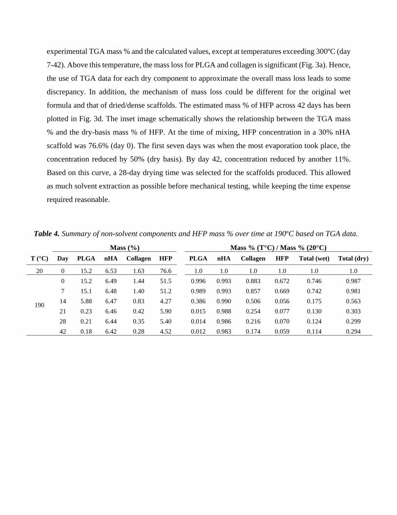
Table 4. Summary of non-solvent components and HFP mass % over time at 190ºC based on TGA data.

Mass (%) Mass % (T°C) / Mass % (20°C)

T (°C) Day PLGA nHA Collagen HFP PLGA nHA Collagen HFP Total (wet) Total (dry)

20 0 15.2 6.53 1.63 76.6 1.0 1.0 1.0 1.0 1.0 1.0

190

0 15.2 6.49 1.44 51.5 0.996 0.993 0.883 0.672 0.746 0.987

7 15.1 6.48 1.40 51.2 0.989 0.993 0.857 0.669 0.742 0.981

14 5.88 6.47 0.83 4.27 0.386 0.990 0.506 0.056 0.175 0.563

21 0.23 6.46 0.42 5.90 0.015 0.988 0.254 0.077 0.130 0.303

28 0.21 6.44 0.35 5.40 0.014 0.986 0.216 0.070 0.124 0.299

42 0.18 6.42 0.28 4.52 0.012 0.983 0.174 0.059 0.114 0.294

Figure 3. (a) Comparison of mass % up to 800C for a 30% nHA formula and the non-solvent

components; (b) TGA mass loss curves for 30% nHA scaffold as it dried for 42 days. The inset

image shows the temperature zone of interest for the calculation of evaporated HFP. (c)

Comparison of the TGA mass % data and the constructed mass % curves (symbols) based on the

approximated HFP loss over time, (d) HFP mass concentration within a 30% nHA scaffold as it

dried for 42 days. HFP concentration was approximated via Eqn. 7 (original basis: TGA%) and

Eqn. 8 (dry basis, with respect to non-solvent components on day 0).

The SEM evaluated the strand width (D) and strand spacing (EtE) for the scaffolds using

the top-down perspective, while the cross-sectional view was used to determine the strand height

(H) in order to estimate the average diameter and porosity of the scaffold. Figure 4a and 4b show

the top-down and cross-sectional SEM views of the scaffolds for run 6 and run 3, respectively.

The estimated porosities of all scaffolds appeared to be over 50% (Table 5). At the lowest spacing

and highest diameter for the 24 runs, the porosities were approximately 56-58% void space.

Figure 4. (a) SEM image of scaffold (run 6) in top-down view, and (b) scaffold (run 3) in cross-

section view.

Table 5. Experimentally determined characteristics of the DE scaffolds.

Run

Number Avg Strand

Diameter (µm) SD

Avg EtE

Spacing (µm) SD

Avg H

(µm) SD

Avg Porosity

(%) SD

Avg Comp.

Modulus (MPa) SD

1 428 12.6 869 16.3 278 10 76.3 0.4 5.44 0.268

2 519 26.9 638 16.2 320 7 62.1 1.9 4.36 0.156

3 318 8.6 552 47.4 273 4 73.7 2.1 2.77 0.206

4 426 32.1 664 35.3 322 7 67.1 1.2 4.85 0.244

5 394 3.2 701 29.3 319 21 70.0 1.7 3.27 0.390

6 358 6.8 860 36.1 267 6 79.4 0.8 1.48 0.184

7 408 6.3 687 40.6 286 15 72.1 0.6 3.22 0.284

8 466 18.0 498 20.1 326 10 58.8 1.1 5.16 0.370

9 376 10.4 717 9.9 318 5 71.5 0.8 2.08 0.123

10 472 18.5 904 17.4 335 10 70.2 2.1 2.40 0.199

11 317 4.9 501 18.1 285 8 71.1 1.1 1.64 0.039

12 363 14.5 886 104.2 285 13 77.7 2.0 0.894 0.015

13 331 12.8 884 30.7 313 13 77.7 1.1 5.69 0.119

14 445 13.6 478 8.0 321 4 59.5 0.7 9.07 0.396

15 363 24.1 1012 22.1 350 8 75.8 1.0 8.48 0.679

16 336 3.1 703 27.5 269 26 77.2 2.7 6.05 0.354

17 402 5.7 683 20.1 284 4 72.5 0.6 2.48 0.113

18 355 17.4 969 13.9 303 7 78.7 1.2 2.06 0.072

19 288 6.0 565 77.0 258 2 77.0 1.9 1.31 0.085

20 445 7.6 744 31.6 322 25 68.4 2.7 3.59 0.197

21 292 5.2 679 100.3 282 16 78.2 1.6 1.80 0.129

22 454 35.7 869 67.2 325 9 70.7 4.2 2.63 0.095

23 473 8.8 478 5.3 335 8 56.3 1.5 3.53 0.188

24 445 13.4 428 27.7 324 9 56.3 3.5 3.10 0.154

The CT image of a 3D scaffold containing 30% nHA is shown in Fig. 5a. Figure 5b

depicts the cross-sectional 2D view of the same scaffold, where the color scale bar represents the

density in g-HA/cm3. Overall, these two images indicate that nHA particles were evenly distributed

throughout the scaffold. The total volume % of the solid matrix was 54% according to the CT

analysis, which translates to a porosity of 46% (void space). Figure 5c gives the 2D view of a

scaffold with 0% nHA, for which the estimated CT porosity was 58%. Finally, Fig. 5d and 5e

demonstrate that over 50% of the density distribution for the 30% nHA scaffold lies between

0.302-0.422 g-HA/cm3, whereas for the 0% nHA scaffold the corresponding density range is

0.109-0.123 g-HA/cm3 (in the absence of nHA particles). These values approximate the density of

the 3DBP strands for these two scaffold compositions. It should be noted that the porosities

estimated for these scaffold topologies using Eqn. 2 were 52% and 66%, respectively. These

estimates were based on their topological dimensions (for 30% nHA: D540 m, EtE570 m,

H380 m, and for 0% nHA: D400 m, EtE610 m, H330 m). Therefore, the porosity

calculated using Eqn. 2 overestimated the actual (CT) porosities by 15%. This is partly due to

a layer thickness (L) smaller than 300 m for the bottom layers of the scaffolds (see Fig. 4b).

Figure 5. (a) The CT image of a 3D scaffold with 30% nHA, and (b and c) the 2D cross-

sectional view of the scaffolds with 30% nHA and 0% nHA, respectively. (d and e) Distribution

% of the density (in g-HA/cm3) throughout the scaffolds. The CT porosities were 46% and 58%

for the two scaffolds, respectively (52% and 66% calculated using Eqn. 2).

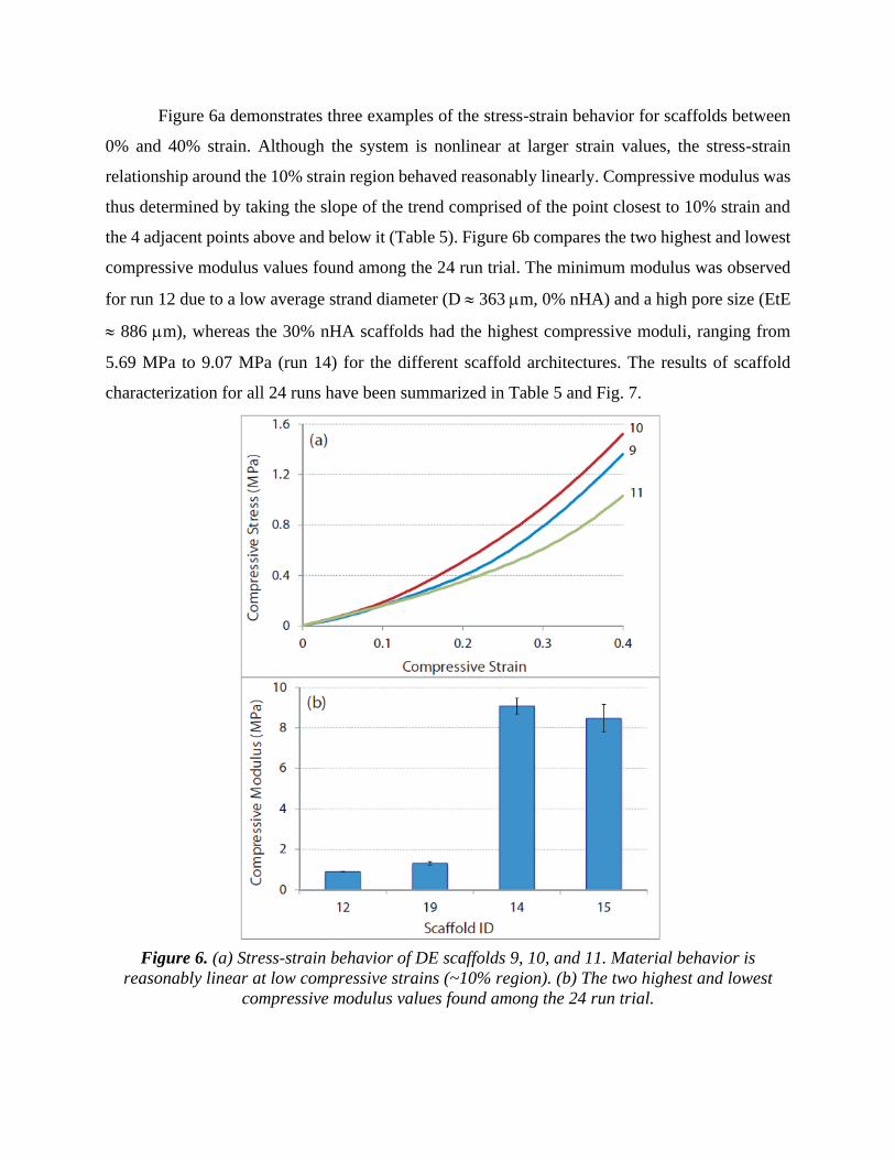
Figure 6a demonstrates three examples of the stress-strain behavior for scaffolds between

0% and 40% strain. Although the system is nonlinear at larger strain values, the stress-strain

relationship around the 10% strain region behaved reasonably linearly. Compressive modulus was

thus determined by taking the slope of the trend comprised of the point closest to 10% strain and

the 4 adjacent points above and below it (Table 5). Figure 6b compares the two highest and lowest

compressive modulus values found among the 24 run trial. The minimum modulus was observed

for run 12 due to a low average strand diameter (D 363 m, 0% nHA) and a high pore size (EtE

886 m), whereas the 30% nHA scaffolds had the highest compressive moduli, ranging from

5.69 MPa to 9.07 MPa (run 14) for the different scaffold architectures. The results of scaffold

characterization for all 24 runs have been summarized in Table 5 and Fig. 7.

Figure 6. (a) Stress-strain behavior of DE scaffolds 9, 10, and 11. Material behavior is

reasonably linear at low compressive strains (~10% region). (b) The two highest and lowest

compressive modulus values found among the 24 run trial.

Optimal scaffold design often aims to maximize either the porosity or the compressive

modulus, subject to certain constraints. Based on the porosity-factor scatter plot (Fig. 7, bottom 3

plots), the average strand diameter and strand spacing appear to have visible effects on porosity.

Plotting the compressive modulus versus the factor values (Fig. 7, top 3 plots) shows that %nHA

appears to have the largest consistent effect on modulus, whereas diameter seems to have a smaller

positive impact. The best scaffold designs for porosity, high spacing and low diameter, were able

to reach over 75%. Based on this, even if the optimal scaffold design for compressive modulus

were to fall in the denser area of the design region, the topology would still satisfy the minimum

porosity of 50%.

Figure 7. Scatter plots of the factor-response relationships: compressive modulus plots (top),

porosity plots (bottom)

3.3 DE Optimization

The fitted split-plot regression models, based on the experimental data in Fig. 7, can be viewed as

second-order approximations of the relationship between the responses and the factors. They are

given as follows:

𝑃𝑟𝑒𝑑𝑖𝑐𝑡𝑒𝑑 𝐶𝑜𝑚𝑝𝑟𝑒𝑠𝑠𝑖𝑣𝑒 𝑀𝑜𝑑𝑢𝑙𝑢𝑠 = 2.94 + 2.76(𝑛) + 1.86(𝑛2) + 1.39(𝑑) + 0.71(𝑛)(𝑑) (9)

𝑃𝑟𝑒𝑑𝑖𝑐𝑡𝑒𝑑 𝑃𝑜𝑟𝑜𝑠𝑖𝑡𝑦 = 75.64 − 5.95(𝑑) + 3.07(𝑠) − 2.31(𝑠2) (10)

𝑛 =[(%𝑛𝐻𝐴)−0.15]

0.15 , 𝑑 =

(𝐷−380)

80 , 𝑠 =

(𝐸𝑡𝐸−800)

200 (11-13)

Equations 9 and 10 have been plotted in Fig. 8, where the solid lines represent the effects

of each factor on a given response (porosity or modulus). The compressive modulus fitted equation

is comprised of a quadratic effect due to %nHA, a linear effect caused by strand diameter, and an

interaction term where the two have a multiplicative effect on the response. The interaction term,

although not as influential as the quadratic effect of %nHA, indicates that the positive effect of

either factor is diminished if the other factor is at a small value. Conceptually, if a 30% nHA

formula were utilized, the use of thin strands would reduce the amount of material present,

mitigating the effect of the material choice. Similarly, high diameter strands are less effective if

they are composed of material with low mechanical strength. Strand spacing was determined to

have a negligible effect on compressive modulus, so it was not included in the model. In

comparison, the porosity fitted model is solely composed of the architectural factors: strand

diameter and strand spacing. Unlike the compressive modulus model, the strand spacing factor has

a quadratic effect on porosity, and strand diameter has a linear effect.

Levels of the factors that predict a maximum modulus with a porosity constrained above

50% are demonstrated in Fig. 8. Based on the DE model and within the design region, our estimate

of the optimal scaffold design is 30% nHA, 460 µm strand diameter, and 923 µm strand spacing.

For nHA composition, selecting the highest level is ideal, as it has the largest effect on compressive

modulus of all factors with no detrimental effect on porosity. Selecting strand spacing is the inverse

scenario: choosing a high spacing has a positive effect on porosity without any detrimental effect

on compressive modulus. (Note that there could be a detrimental effect, but our experimental data

suggested this effect would be negligible.) Strand diameter is the only factor that affects both

responses, according to our empirical model. It is possible to choose the maximum diameter for

its positive effect on compressive modulus since the porosity response is still within acceptable

bounds. The experimental models predict that, for this optimized design, the resultant scaffold

would have a compressive modulus of 9.66 MPa, and a porosity of 70.7%. This porosity is highly

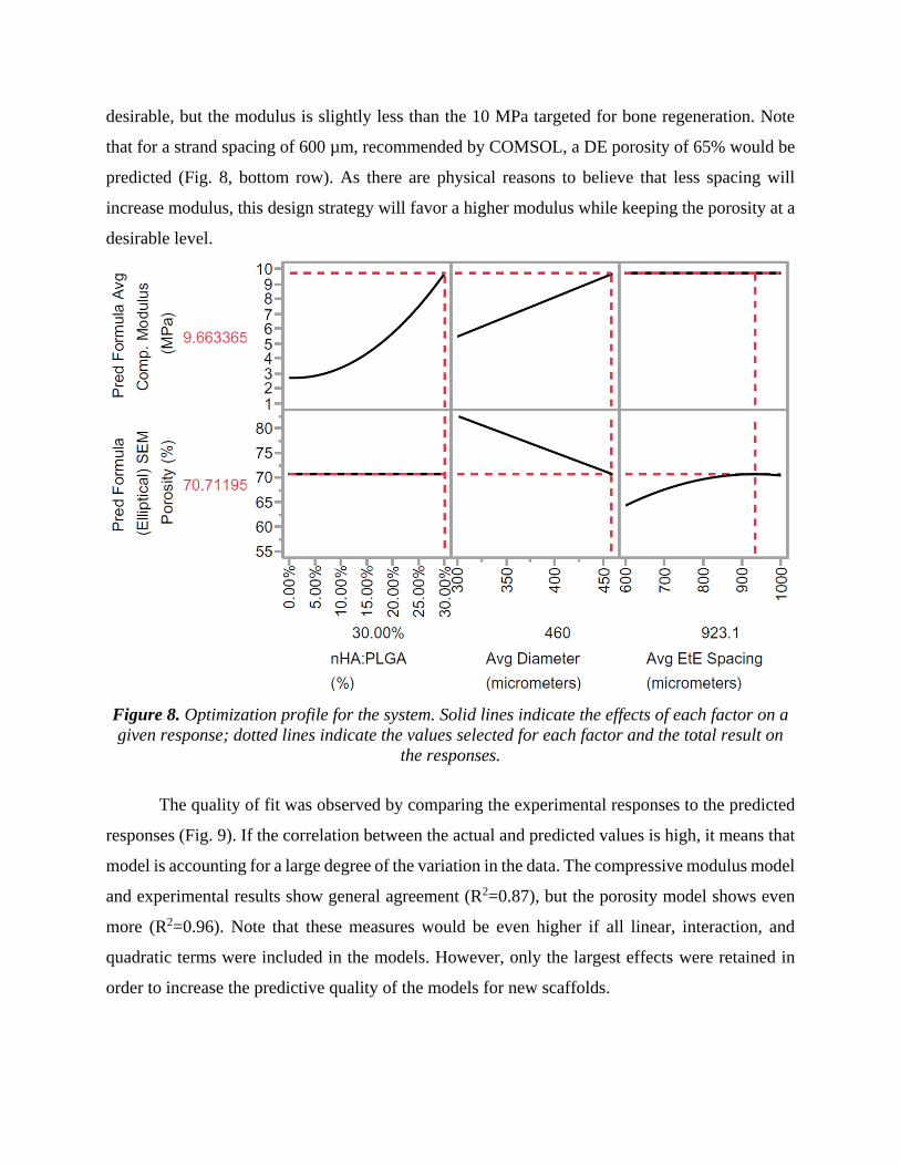
desirable, but the modulus is slightly less than the 10 MPa targeted for bone regeneration. Note

that for a strand spacing of 600 µm, recommended by COMSOL, a DE porosity of 65% would be

predicted (Fig. 8, bottom row). As there are physical reasons to believe that less spacing will

increase modulus, this design strategy will favor a higher modulus while keeping the porosity at a

desirable level.

Figure 8. Optimization profile for the system. Solid lines indicate the effects of each factor on a

given response; dotted lines indicate the values selected for each factor and the total result on

the responses.

The quality of fit was observed by comparing the experimental responses to the predicted

responses (Fig. 9). If the correlation between the actual and predicted values is high, it means that

model is accounting for a large degree of the variation in the data. The compressive modulus model

and experimental results show general agreement (R2=0.87), but the porosity model shows even

more (R2=0.96). Note that these measures would be even higher if all linear, interaction, and

quadratic terms were included in the models. However, only the largest effects were retained in

order to increase the predictive quality of the models for new scaffolds.

Figure 9. Plots of experimental response versus predicted response for (a) compressive modulus

and (b) porosity.

3.4 COMSOL Optimization

Optimizations were run at three levels of compressive modulus (E) corresponding to the three

%nHA levels. All three optimizations iterated through the same topologies, and finished at a

topology of 460 µm strand diameter and 601 µm strand spacing (Table 6). As the architectural

factors were identical, the three simulations agreed upon a resultant porosity of 54.3%. The

predicted compressive moduli, however, varied according to the assumed ceramic composition,

improving as %nHA did. At the highest nHA level, the predicted compressive modulus was 5.67

MPa. Figure 10 shows the surface plot of the stress experienced at the top surface of the scaffold

model. As the color bar indicates, the peaks of stress are in alignment with the strands of the

previous layer.

Table 6. Abridged results of COMSOL optimization. The module began at the same diameter

and strand spacing, and searched in the same order for 30 iterations.

Iteration Strand Diameter

(µm)

Strand Spacing

(µm) Porosity (%)

Compressive Modulus (MPa)

0% nHA 15% nHA 30% nHA

1 380 800 65.2 0.32 1.63 4.03

5 416 710 60.8 0.36 1.85 4.59

10 431 659 58.9 0.39 2.00 4.95

15 454 605 54.7 0.44 2.25 5.58

20 457 600 54.3 0.45 2.27 5.63

25 459 601 54.3 0.45 2.28 5.65

30 460 601 54.3 0.45 2.29 5.67

Figure 10. Surface plot of the stress experienced at the top surface of the scaffold model. Peaks

of stress are in alignment with the strands of the previous layer.

3.5 Validation Results

Seven 30% nHA scaffolds were plotted in order to validate the predictions of DE and COMSOL

models (Table 7). Figure 11a and 11b compare the two models with respect to their modulus

predictions and porosity estimations, while Figure 11c and 11d depict their absolute percentage

errors, respectively. The mean absolute percentage error (MAPE) was calculated for the DE

predictions and COMSOL simulations. With regards to porosity estimation for the seven validation

scaffolds, the DE model had a MAPE of about 4%. COMSOL, on the other hand, had a MAPE of

13% and consistently underestimated the scaffold porosity. This may be due to how the simulation

utilizes a constant layer overlap parameter (L/H=0.7). However, this ratio tends to vary,

particularly in bottom layers close to the plotting platform. Another factor that could contribute to

underestimated porosity was that each strand in COMSOL was defined as a cylinder of circular

cross-section (average D) to accommodate the iterative optimization process. It should be noted

that, as CT results indicated, Eqn. 2 tends to overestimate the experimental (SEM) porosity by

∼15%. Therefore, the COMSOL porosities could still offer good estimates for the actual porosities

of these scaffolds (L/H=0.7). Nevertheless, when experimental L/H (0.56 - 1.0 from SEM) were

used in the simulations, COMSOL substantially underestimated the measured porosities for L/H

< 0.7 (Table 7). This is because at a high layer overlap, the shape of strands tends to deviate even

further from a circular cross-section.

Table 7. Comparison between the experimentally determined validation scaffold physical

characteristics and the predicted results based on Eqs. 9 and 10 (DE) and the COMSOL model.

nHA

(%)

Avg.

Diam.

(µm)

Avg.

ETE

(µm)

SEM

L/H

Experimental

Modulus

(MPa)

DE

Predicted

Modulus

(MPa)

COMSOL

Predicted

Modulus

(L/H = 0.70)

(MPa)

COMSOL

Predicted

Modulus

(SEM L/H)

(MPa)

Experimental

Porosity

(%)

DE

Predicted

Porosity

(%)

COMSOL

Porosity

(L/H = 0.70)

(%)

COMSOL

Porosity

(SEM L/H)

(%)

30% 416 ± 8 555 ± 16 0.66 5.07 ± 0.17 8.51 5.36 6.09 71.4 ± 1.8 65.7 55.3 53.0

30% 425 ± 16 555 ± 12 0.70 5.10 ± 0.10 8.74 5.46 5.46 65.4 ± 0.3 65.1 54.7 54.7

30% 333 ± 4 932 ± 9 1.00 5.48 ± 0.13 6.33 3.5 0.14 81.9 ± 0.9 80.1 71.0 78.9

30% 309 ± 20 981 ± 11 1.00 5.89 ± 0.19 5.69 3.16 0.14 83.6 ± 1.4 81.8 74.3 81.1

30% 469 ± 8 851 ± 53 -- 5.23 ± 0.34 9.91 4.67 -- 68.5 ± 2.2 69.6 62.3 --

30% 482 ± 18 525 ± 17 0.56 9.92 ± 1.16 10.3 6.07 7.77 54.1 ± 1.2 59.4 50.1 41.9

30% 460 ± 28 864 ± 48 -- 4.52 ± 1.52 9.66 4.58 -- 69.5 ± 1.6 70.5 63.0 --

Figure 11. (a & b) Comparison between the COMSOL and DE porosities and moduli for the validation

scaffolds, (c & d) comparison of their absolute error (%) for porosity estimations and modulus

predictions, respectively. These COMSOL simulations were for a constant layer overlap (L/H = 0.7).

The DE model fared worse in predicting the moduli for the seven validation scaffolds.

However, the moduli predicted by the DE model agreed well with the experimental values when

the strand diameter (D) was the dominant factor affecting the scaffold modulus (at very low or

very high D values: sample 3, 4, and 6). The experimental modulus values were within 16% of

the DE prediction values in these three cases, whereas the mean absolute prediction error for all

seven validation scaffolds was 52%. This is not surprising as L/H ratio was not accounted for in

the DE model, while EtE spacing had no effect on the DE model response (see Fig. 8 and Table

3). In practice, it is a tremendous challenge to use L/H as an independent DE factor, as it is highly

affected by the rheological properties of the formula, plotting speed, plotting pressure, and the

dispensing needle diameter. COMSOL was better at predicting the modulus than the designed

experiment. Overall, COMSOL better predicted the modulus when the scaffold had an

intermediate experimental porosity range (65 - 71%, sample 1, 2, 5 and 7). The experimental

modulus values were within 11% of the COMSOL prediction values in these four cases (for

L/D=0.7), whereas the mean absolute prediction error for all seven samples was 21%.

COMSOL simulations using variable L/H (from SEM) highly under-predicted the modulus

of sample 3 and 4 (> 30% absolute error). The lack of overlap between the successive layers

(L/H=1) led to a significant drop in the predicted COMSOL modulus. It should be noted that

sample 3 and 4 had higher compressive moduli than scaffolds in the low end of the porosity range

(e.g., sample 1 and 2). As noted previously, solvent is still present within the scaffolds even after

28 days of drying. It may be possible that due to the increased EtE spacing (> 900 m) and low

strand diameter (D < 350 m), sample 3 and 4 had improved solvent evaporation rates, which

would contribute to the overall mechanical performance of the scaffold. In case of sample 6, the

porosity and L/H values were the lowest of all the validation scaffolds, so it had the highest

compressive modulus (in agreement with the DE model). An L/H value close to 0.5 represents a

very dense scaffold with highly overlapping layers. Thus, sample 6 showed an experimental

modulus similar to a solid block for this formula. This scaffold was much denser at its bottom

layers, which cannot be realistically replicated in a COMSOL model. The SEM L/H values used

in the simulations were only reflective of the middle-to-top layers of the actual scaffolds.

3.6 Methodology Comparison

The two models suggested using the highest values for strand diameter and nHA content. However,

the experimental model found the effect of strand spacing on modulus to be insignificant, while

the simulation predicted an improvement to modulus by reducing the spacing and increasing the

number of strands per layer as a result. That said, the spacing only has an effect on porosity in the

experimental model, so it would be feasible to use the topology suggested by COMSOL because

the reduction in porosity would still fall within the acceptable bounds according to the

experimental model.

4 Discussion

Composites made of collagen and hydroxyapatite (HA) are attractive biocompatible materials as

they possess the organic and mineral constituents of bone [46–48]. Scaffolds made of collagen and

HA with/without synthetic polymers have been widely produced by electrospinning (ES) [49–52]

and conventional scaffold fabrication techniques [53–57]. The flexibility of generating broad pore

size ranges and mechanical properties by additive manufacturing (AM) makes it a superior

alternative to ES and conventional techniques [58–61]. Hence, this work investigated the

mechanical properties of PLGA-nHA-collagen composite scaffolds produced by 3D bioplotting

(3DBP) using HFP as a solvent. The amount of solvent retention was quantified over scaffold

drying time (0-42 days) based on mass balance principles and thermogravimetric analysis (TGA).

The methodology presented herein required a small sample size and could assist researchers in

analyzing solvent retention in tissue-engineering scaffolds and other biomaterials.

A fundamental requirement for tissue-engineered bone grafts is the ability to integrate with

the host tissues while providing the capacity for remodeling and load-bearing [62,63]. The rapid

restoration of biomechanical function is crucial in functional TE, emphasizing the need for optimal

scaffold designs [64–66]. In recent years, finite element (FE) modeling has been extensively used

to design 3D scaffolds by a variety of AM techniques [8,32,33,37,38,63,67]. Designed experiment

(DE) have also been used for scaffold design, by accounting for a multitude of factors affecting

the physical performance and biological outcomes of 3D scaffolds [21,68–70].

The aim of this study was to compare the FE and DE methods for the design of bone TE

scaffolds. Computational over-prediction of scaffold performance has been partly attributed to the

presence of a micro-topology on the surface of scaffolds that has not been accounted for in

simulation models, and it has been suggested that the architecture of the scaffold affects the degree

of the impact [36,38]. The COMSOL model presented here under-predicted compressive modulus

of the scaffolds in 5 validation cases (out of 7). In comparison to other AM methods, such as

sintering, scaffolds produced by 3D bioplotting have distinctly smooth surfaces [6]. Thus, it is

possible that the lack of a micro-topology reduced the risk of over-prediction by the COMSOL

model.

The prediction capability of FE models also depends on the range of applied compressive

strains. For an idealized simple cubic strand layout (L/H = 1, no overlap between layers), it has

been reported that FE simulations tend to under-predict the absolute values of compressive stress

at low strains (<30%) due to inter-layer overlap that contributes to higher experimental stresses.

On the other hand, FE simulations tend to over-predict stress at high strains due to buckling effects

[71]. Hence, the symmetry constraint used in the simulation of scaffold compression is more likely

to be violated under actual test conditions [71]. In our study, COMSOL simulations considerably

under-predicted the modulus of two validation samples (#3 and #4, L/H = 1). In an extreme case

(our #6 validation sample), the significant increase in the solid fraction of the actual scaffold at

bottom layers, compared to the simulated one, contributed to the pronounced discrepancy between

the experimental and predicted moduli. The SEM L/H values used in the simulations were only

reflective of the middle-to-top layers of the actual scaffolds.

In this study, both the experimental (DE) and computational (FE) model suggested the

maximum %nHA value (30%) in order to improve compressive modulus of the scaffolds.

Researchers often incorporate the harder HA phase into a polymer matrix to improve its

mechanical properties [72–74]. However, in some cases the addition of HA may not increase the

properties over that of the monolithic polymer [73]. For example, it has been reported that nHA

concentrations above 20 wt% can decrease the compressive modulus of PLGA-nHA composites

[28]. As such, while the lack of a maximum peak within our design region may suggest examining

a larger %nHA, it may not produce an improvement in compressive modulus. In general,

differences in experimental methods used for adding nHA particles to polymers (such as particle

size, agglomeration of particles, and polymer/filler interfaces) may affect the final properties of

the composite. Dispersion of ceramic particles into a polymer solution followed by consolidation

(solvent casting) has been considered as a means of improving the polymer/filler interfaces

[75,76]. This may explain the increase in compressive modulus of our scaffolds at 30% nHA. In

situ precipitation has also shown to improve the mechanical properties of polymer composites at

high nHA contents [77], when compared to similar composite systems [78–80]. It should be noted

that there is not a consensus on the optimal range of scaffold modulus for bone tissue engineering,

as the reported values highly vary depending on the scaffold material and architecture used for in

vitro and in vivo studies [2,81,82].

Both FE and DE models also suggested maximizing the strand diameter of scaffolds, and

agreed that the factor has a positive effect on compressive modulus and a negative effect on

porosity. This behavior is consistent with the study performed by Giannitelli et al. (2014), who

also found that increasing strand diameter of their model, while holding all other aspects of the

topology constant, caused an increase in stiffness and reduced porosity [7]. However, FE and DE

models conflicted on the optimal strand spacing value. The experimental model nearly maximized

spacing because it found no statistically relevant effect on the compressive modulus, but COMSOL

minimized spacing in order to improve the modulus. As the COMSOL sensitivity analysis

indicated (Table 3), an increase in strand spacing has a smaller effect on the scaffold modulus (<

1.5 MPa net change] for a compliant scaffold material (E < 12 MPa for our 3 formulae], when

compared to the net change in scaffold modulus (> 25 MPa) for a stiffer solid matrix (E > 100

MPa). In light of this, the DE model should be able to readily capture the effect of strand spacing

for scaffolds made of stiffer materials.

The negative impact of porosity on compressive modulus is well established [7,20,83]. Any

factor that affects porosity, such as strand spacing, should affect the modulus as well. Giannitelli

et al. (2014) examined the effect of strand spacing on their simulation model and found that (even

when porosity was held constant) larger strand spacing values reduced scaffold stiffness [7]. The

cause of this disagreement between our two models may be further indicated by Fig. 12, which

outlines the compressive modulus predicted by COMSOL as it iterated across the design region.

At iteration 10, COMSOL increased porosity by increasing strand spacing and decreasing

diameter. This resulted in a decrease in compressive modulus; however, the degree of impact was

dependent on the material assumed. The 30% material (with the largest compressive modulus)

suffered the largest loss in compressive modulus, whereas the 0% nHA simulation was less

affected.

Figure 12. Compressive modulus of COMSOL scaffold model across iterations of the

optimization process.

It has been recommended that bone tissue scaffolds have a minimum pore size of 300 µm

[20,66,84]. Although, it has been suggested by Fisher et al. (2002) that pore sizes up to 800 µm

perform similarly to 300 µm pores in vivo [85]. This supports the use of the strand spacing

suggested by COMSOL, but not the spacing recommended by the experimental model. In addition,

the use of such a large spacing may cause a significant lack of surface area available for cellular

attachment. Thus, it may be more beneficial to consider a smaller strand spacing than the

experimental model suggests. Such a decision still produces scaffolds with acceptable porosities,

because the experimental model indicated that all the strand spacing values within the design

region resulted in porosities greater than 50%. The impact of large pore sizes on the accuracy of

FE simulations should be further investigated in future studies. Size effects matter, particularly

when the microstructural length scale of the porous material approaches the macroscale

dimensions of the sample [86].

5 Conclusions

A 3D bioplotter was used to produce 24 bone tissue scaffolds according to a split-plot designed

experiment (DE). These scaffolds were made of PLGA, nHA and type I collagen using HFP as a

solvent. Mathematical models were generated relating nHA content and strand diameter to

compressive modulus, and strand diameter and spacing to porosity. An optimized scaffold design

generated from the experimental data was compared to an optimal design given by the COMSOL

optimization module. Seven validation scaffolds were produced to cover COMSOL and DE

optimal design ranges. These scaffolds had measured moduli between 4.5-9.9 MPa, depending on

strand diameter, spacing and layer overlap.

The main hypothesis of this study was that both the experimental (DE) and COMSOL (FE)

models should suggest similar optimal topologies (±20% design factor value agreement). Within

the design region, the DE and COMSOL models agreed in their recommended optimal nHA (30%)

and strand diameter (460 µm). However, the two methods disagreed by more than 20% in strand

spacing (923 µm for DE; 601 µm for COMSOL), for reasons discussed previously in this paper.

The predicted results for the seven validation scaffolds showed relative agreement for scaffold

porosity (mean absolute percentage error of 4% for DE and 13% for COMSOL), but the predictions

were substantially poorer for scaffold modulus (52% for DE; 21% for COMSOL).

Topology optimization has a great potential in improving the efficiency of scaffold design,

even in cases where the property values are over/under-predicted. Expanding the design region in

future experiments (e.g., higher nHA content and strand diameter), developing a more efficient

solvent evaporation method, and exerting a greater control over layer overlap could allow

developing PLGA-nHA-collagen scaffolds to meet the mechanical requirements for bone TE.

6 Acknowledgements

This work was partially funded by the Ohio Board of Regents, the Ohio Third Frontier Program

grant entitled: “Ohio Research Scholars in Layered Sensing”, IDCAST, Miami University’s Office

for the Advancement of Research (OARS), and the College of Engineering and Computing (CEC).

The authors wish to thank DSM Biomedical (Exton, PA) for generously supplying type 1 collagen

used in this study. The authors also wish to thank Kathleen LaSance from the University of

Cincinnati for CT analysis, Dr. Justin Saul for rheological measurements, Dr. Catherine

Almquist, Dr. Jessica Sparks, Doug Hart, Matt Duley, Judy Bohnert, Rosa Akbarzadeh, Cara

Janney and Carlie Focke for their technical assistance, and Laurie Edwards for her administrative

assistance.

References

1. Razi H, Checa S, Schaser K-D, Duda GN. Shaping scaffold structures in rapid manufacturing

implants: a modeling approach toward mechano-biologically optimized configurations for large

bone defect. J Biomed Mater Res B Appl Biomater. 2012 Oct;100(7):1736–45.

http://www.ncbi.nlm.nih.gov/pubmed/22807248

2. Hollister SJ. Porous scaffold design for tissue engineering. Nat Mater. 2005 Jul;4(7):518–24.


3. Brydone AS, Meek D, Maclaine S. Bone grafting, orthopaedic biomaterials, and the clinical need

for bone engineering. Proc Inst Mech Eng Part H J Eng Med . 2010 Dec 1;224 (12):1329–43.

http://pih.sagepub.com/content/224/12/1329.abstract

4. Liu X, Ma PX. Polymeric scaffolds for bone tissue engineering. Ann Biomed Eng. 2004

Mar;32(3):477–86.

5. Sachlos E, Czernuszka JT. Making tissue engineering scaffolds work. Review: the application of

solid freeform fabrication technology to the production of tissue engineering scaffolds. Eur Cell

Mater. 2003 Jun;5:29–40.

6. Yeong W-Y, Chua C-K, Leong K-F, Chandrasekaran M. Rapid prototyping in tissue engineering:

challenges and potential. Trends Biotechnol. 2004 Dec;22(12):643–52.


7. Giannitelli SM, Rainer A, Accoto D, De Porcellinis S, De-Juan-Pardo EM, Guglielmelli E, et al.

Optimization Approaches for the Design of Additively Manufactured Scaffolds. In: Fernandes RP,

Bartolo JP, editors. Tissue Engineering: Computer Modeling, Biofabrication and Cell Behavior.

Dordrecht: Springer Netherlands; 2014. p. 113–28. http://dx.doi.org/10.1007/978-94-007-7073-7_6

8. Boccaccio A, Ballini A, Pappalettere C, Tullo D, Cantore S, Desiate A. Finite element method

(FEM), mechanobiology and biomimetic scaffolds in bone tissue engineering. Int J Biol Sci. 2011

Jan;7(1):112–32.

http://www.pubmedcentral.nih.gov/articlerender.fcgi?artid=3030147&tool=pmcentrez&rendertype

=abstract

9. Kelly DJ, Prendergast PJ. Prediction of the optimal mechanical properties for a scaffold used in

osteochondral defect repair. Tissue Eng. 2006 Sep;12(9):2509–19.


10. Ngiam M, Liao S, Patil AJ, Cheng Z, Chan CK, Ramakrishna S. The fabrication of nano-

hydroxyapatite on PLGA and PLGA/collagen nanofibrous composite scaffolds and their effects in

osteoblastic behavior for bone tissue engineering. Bone. 2009 Jul;45(1):4–16.


11. Sandino C, Lacroix D. A dynamical study of the mechanical stimuli and tissue differentiation within

a CaP scaffold based on micro-CT finite element models. Biomech Model Mechanobiol. 2011

Jul;10(4):565–76. http://www.ncbi.nlm.nih.gov/pubmed/20865437

12. Hsieh W-T, Liu Y-S, Lee Y, Rimando MG, Lin K, Lee OK. Matrix dimensionality and stiffness

cooperatively regulate osteogenesis of mesenchymal stromal cells. Acta Biomater. 2016;32:210–22.

13. Checa S, Prendergast PJ. A mechanobiological model for tissue differentiation that includes

angiogenesis: a lattice-based modeling approach. Ann Biomed Eng. 2009 Jan;37(1):129–45.


14. Khayyeri H, Checa S, Tägil M, O’Brien FJ, Prendergast PJ. Tissue differentiation in an in vivo

bioreactor: in silico investigations of scaffold stiffness. J Mater Sci Mater Med. 2010

Aug;21(8):2331–6. http://www.ncbi.nlm.nih.gov/pubmed/20037774

15. Hollister SJ, Maddox RD, Taboas JM. Optimal design and fabrication of scaffolds to mimic tissue

properties and satisfy biological constraints. Biomaterials. 2002 Oct;23(20):4095–103.


16. Sanz-Herrera JA, García-Aznar JM, Doblaré M. On scaffold designing for bone regeneration: A

computational multiscale approach. Acta Biomater. 2009 Jan;5(1):219–29.


17. Milan J-L, Planell J a, Lacroix D. Simulation of bone tissue formation within a porous scaffold

under dynamic compression. Biomech Model Mechanobiol. 2010 Oct;9(5):583–96.


18. Rho JY, Ashman RB, Turner CH. Young’s modulus of trabecular and cortical bone material:

ultrasonic and microtensile measurements. J Biomech. 1993 Feb;26(2):111–9.

19. Schaffler MB, Burr DB. Stiffness of compact bone: effects of porosity and density. J Biomech.

1988;21(1):13–6.

20. Karageorgiou V, Kaplan D. Porosity of 3D biomaterial scaffolds and osteogenesis. Biomaterials.

2005;26(27):5474–91. http://linkinghub.elsevier.com/retrieve/pii/S0142961205001511

21. Kim JY, Cho D-W. The optimization of hybrid scaffold fabrication process in precision deposition

system using design of experiments. Microsyst Technol. 2008 Nov 4;15(6):843–51.

http://link.springer.com/10.1007/s00542-008-0727-8

22. Kim S-S, Sun Park M, Jeon O, Yong Choi C, Kim B-S. Poly(lactide-co-glycolide)/hydroxyapatite

composite scaffolds for bone tissue engineering. Biomaterials. 2006;27(8):1399–409.

23. Gentile P, Chiono V, Carmagnola I, Hatton P V. An Overview of Poly(lactic-co-glycolic) Acid

(PLGA)-Based Biomaterials for Bone Tissue Engineering. Int J Mol Sci. 2014;15(3):3640.

http://www.mdpi.com/1422-0067/15/3/3640

24. Marra KG, Szem JW, Kumta PN, DiMilla PA, Weiss LE. In vitro analysis of biodegradable polymer

blend/hydroxyapatite composites for bone tissue engineering. J Biomed Mater Res. 1999

Dec;47(3):324–35.

25. Orlovskii VP, Komlev VS, Barinov SM. Hydroxyapatite and Hydroxyapatite-Based Ceramics.

Inorg Mater. 2002;38(10):973–84. http://dx.doi.org/10.1023/A:1020585800572

26. Wang H. Hydroxyapatite degradation and biocompatibility. Ohio State University; 2004.

27. Jose M V, Thomas V, Xu Y, Bellis S, Nyairo E, Dean D. Aligned bioactive multi-component

nanofibrous nanocomposite scaffolds for bone tissue engineering. Macromol Biosci. 2010

Apr;10(4):433–44.

28. Shuai C, Yang B, Peng S, Li Z. Development of composite porous scaffolds based on poly(lactide-

co-glycolide)/nano-hydroxyapatite via selective laser sintering. Int J Adv Manuf Technol.

2013;69(1):51–7. http://dx.doi.org/10.1007/s00170-013-5001-2

29. Lai ES, Anderson CM, Fuller GG. Designing a tubular matrix of oriented collagen fibrils for tissue

engineering. Acta Biomater. 2011 Jun;7(6):2448–56.

30. Barnes CP, Pemble CW, Brand DD, Simpson DG, Bowlin GL. Cross-linking electrospun type II

collagen tissue engineering scaffolds with carbodiimide in ethanol. Tissue Eng. 2007

Jul;13(7):1593–605. http://www.ncbi.nlm.nih.gov/pubmed/17523878

31. Matthews JA, Wnek GE, Simpson DG, Bowlin GL. Electrospinning of collagen nanofibers.

Biomacromolecules. 2002;3(2):232–8.

32. Lacroix D, Planell JA, Prendergast PJ. Computer-aided design and finite-element modelling of

biomaterial scaffolds for bone tissue engineering. Philos Trans A Math Phys Eng Sci. 2009 May

28;367(1895):1993–2009. http://www.ncbi.nlm.nih.gov/pubmed/19380322

33. Giannitelli SM, Accoto D, Trombetta M, Rainer A. Current trends in the design of scaffolds for

computer-aided tissue engineering. Acta Biomater. 2014 Feb;10(2):580–94.


34. McIntosh L, Cordell JM, Wagoner Johnson a J. Impact of bone geometry on effective properties of

bone scaffolds. Acta Biomater. 2009 Feb;5(2):680–92.


35. Melchels FP, Bertoldi K, Gabbrielli R, Velders AH, Feijen J, Grijpma DW. Mathematically defined

tissue engineering scaffold architectures prepared by stereolithography. Biomaterials. 2010

Sep;31(27):6909–16. http://www.ncbi.nlm.nih.gov/pubmed/20579724

36. Cahill S, Lohfeld S, McHugh PE. Finite element predictions compared to experimental results for

the effective modulus of bone tissue engineering scaffolds fabricated by selective laser sintering. J

Mater Sci Mater Med. 2009 Jun;20(6):1255–62. http://www.ncbi.nlm.nih.gov/pubmed/19199109

37. Rainer A, Giannitelli SM, Accoto D, De Porcellinis S, Guglielmelli E, Trombetta M. Load-adaptive

scaffold architecturing: a bioinspired approach to the design of porous additively manufactured

scaffolds with optimized mechanical properties. Ann Biomed Eng. 2012 Apr;40(4):966–75.


38. Doyle H, Lohfeld S, McHugh P. Predicting the Elastic Properties of Selective Laser Sintered PCL/β-

TCP Bone Scaffold Materials Using Computational Modelling. Ann Biomed Eng. 2013 Sep

21;42(3):661–77. http://www.ncbi.nlm.nih.gov/pubmed/24057867

39. Blecha LD, Rakotomanana L, Razafimahery F, Terrier A, Pioletti DP. Targeted mechanical

properties for optimal fluid motion inside artificial bone substitutes. J Orthop Res. 2009

Aug;27(8):1082–7.

40. Raymond H. Myers, Douglas C. Montgomery CMA-C. Response Surface Methodology: Process

and Product Optimization Using Designed Experiments. Edition 4th, editor. New York: Wiley;

2016.

41. Wu CFJ, Hamada MS. Experiments: Planning, Analysis, and Optimization. 2nd Editio. New York:

Wiley; 2009.

42. Goos P, Jones B. Optimal Design of Experiments: A Case Study Approach. Hoboken, NJ; 2011.

43. Jones B, Nachtsheim CJ. Split-Plot Designs : What, Why, and How. J Qual Technol.

2009;41(4):340–61.

44. Akkouch A, Zhang Z, Rouabhia M. A novel collagen/hydroxyapatite/poly(lactide-co-ε-

caprolactone) biodegradable and bioactive 3D porous scaffold for bone regeneration. J Biomed

Mater Res Part A. 2011;96A(4):693–704. http://dx.doi.org/10.1002/jbm.a.33033

45. Landers R, Pfister A, Hübner U, John H, Schmelzeisen R, Mülhaupt R. Fabrication of soft tissue

engineering scaffolds by means of rapid prototyping techniques. J Mater Sci. 2002;37(15):3107–16.

http://dx.doi.org/10.1023/A:1016189724389

46. Banglmaier RF, Sander EA, Vandevord PJ. Induction and quantification of collagen fiber alignment

in a three-dimensional hydroxyapatite-collagen composite scaffold. Acta Biomater. 2015;17:26–35.

http://dx.doi.org/10.1016/j.actbio.2015.01.033

47. David F, Levingstone TJ, Schneeweiss W, de Swarte M, Jahns H, Gleeson JP, et al. Enhanced bone

healing using collagen–hydroxyapatite scaffold implantation in the treatment of a large

multiloculated mandibular aneurysmal bone cyst in a thoroughbred filly. J Tissue Eng Regen Med.

2015;9(10):1193–9. http://dx.doi.org/10.1002/term.2006

48. Quinlan E, Thompson EM, Matsiko A, O’Brien FJ, López-Noriega A. Functionalization of a

Collagen–Hydroxyapatite Scaffold with Osteostatin to Facilitate Enhanced Bone Regeneration. Adv

Healthc Mater. 2015;4(17):2649–56. http://dx.doi.org/10.1002/adhm.201500439

49. Tang Y, Chen L, Zhao K, Wu Z, Wang Y, Tan Q. Fabrication of PLGA/HA (core)-

collagen/amoxicillin (shell) nanofiber membranes through coaxial electrospinning for guided tissue

regeneration. Compos Sci Technol. 2016;125:100–7.

50. Kwak S, Haider A, Gupta KC, Kim S, Kang I-K. Micro/Nano Multilayered Scaffolds of PLGA and

Collagen by Alternately Electrospinning for Bone Tissue Engineering. Nanoscale Res Lett.

2016;11(1):1–16. http://dx.doi.org/10.1186/s11671-016-1532-4

51. Zhou Y, Yao H, Wang J, Wang D, Liu Q, Li Z. Greener synthesis of electrospun collagen/

hydroxyapatite composite fibers with an excellent microstructure for bone tissue engineering. Int J

Nanomedicine. 2015;10:3203–15.

52. Ribeiro N, Sousa SR, van Blitterswijk CA, Moroni L, Monteiro FJ. A biocomposite of collagen

nanofibers and nanohydroxyapatite for bone regeneration. Biofabrication. 2014;6(3):35015.

http://stacks.iop.org/1758-5090/6/i=3/a=035015

53. Murphy CM, Schindeler A, Gleeson JP, Yu NYC, Cantrill LC. A collagen–hydroxyapatite scaffold

allows for binding and co-delivery of recombinant bone morphogenetic proteins and

bisphosphonates. Acta Biomater. 2014;10(5):2250–8.

54. Villa MM, Wang L, Huang J, Rowe DW, Wei M. Bone tissue engineering with a collagen–

hydroxyapatite scaffold and culture expanded bone marrow stromal cells. J Biomed Mater Res Part

B Appl Biomater. 2015;103(2):243–53. http://dx.doi.org/10.1002/jbm.b.33225

55. Kon E, Delcogliano M, Filardo G, Busacca M, Di Martino A, Marcacci M. Novel nano-composite

multilayered biomaterial for osteochondral regeneration: a pilot clinical trial. Am J Sports Med.

2011 Jun;39(6):1180–90. http://www.ncbi.nlm.nih.gov/pubmed/21310939

56. Zhou C, Ye X, Fan Y, Ma L, Tan Y, Qing F, et al. Biomimetic fabrication of a three-level

hierarchical calcium phosphate/collagen/hydroxyapatite scaffold for bone tissue engineering.

Biofabrication. 2014;6(3):035013. http://www.ncbi.nlm.nih.gov/pubmed/24873777

57. Akkouch A, Zhang Z, Rouabhia M. Engineering bone tissue using human dental pulp stem cells and

an osteogenic collagen-hydroxyapatite-poly (L-lactide-co-ε-caprolactone) scaffold. J Biomater

Appl. 2014;28(6):922–36. http://www.ncbi.nlm.nih.gov/pubmed/23640860

58. Liu W, Wang D, Huang J, Wei Y, Xiong J, Zhu W, et al. Low-temperature deposition

manufacturing: A novel and promising rapid prototyping technology for the fabrication of tissue-

engineered scaffold. Mater Sci Eng C. 2016;

59. El-Ayoubi R, Eliopoulos N, Diraddo R, Galipeau J, Yousefi A-M. Design and Fabrication of 3D

Porous Scaffolds to Facilitate Cell-Based Gene Therapy. Tissue Eng Part A. 2008 Jun;14(6):1037–

48. http://www.liebertonline.com/doi/abs/10.1089/ten.tea.2006.0418

60. Coutu DL, Yousefi AM, Galipeau J. Three-dimensional porous scaffolds at the crossroads of tissue

engineering and cell-based gene therapy. J Cell Biochem. 2009 Oct 15;108(3):537–46.


61. Yousefi AM, Gauvin C, Sun L, Diraddo RW, Fernandes J. Design and Fabrication of 3D-Plotted

Polymeric Scaffolds in Functional Tissue Engineering. Polym Eng Sci. 2007;47(5):608–18.

62. Bhumiratana S, Vunjak-Novakovic G. Concise Review: Personalized human bone grafts for

reconstructing head and face, stem cells translational medicine. Stem Cells Transl Med. 2012;1:64–

9.

63. Yousefi AM, Hoque ME, Prasad RGS V., Uth N. Current strategies in multiphasic scaffold design

for osteochondral tissue engineering: A review. J Biomed Mater Res Part A. 2015;103(7):2460–81.

http://doi.wiley.com/10.1002/jbm.a.35356

64. Guilak F, Butler DL, Goldstein SA, Money D (Eds. . Functional Tissue Engineering. New York:

Springer; 2003.

65. Ingber DE, Mow VC, Butler D, Niklason L, Huard J, Mao J, et al. Tissue engineering and

developmental biology: going biomimetic. Tissue Eng. 2006 Dec;12(12):3265–83.


66. Akbarzadeh R, Minton JA, Janney CS, Smith TA, James PF, Yousefi AM. Hierarchical polymeric

scaffolds support the growth of MC3T3-E1 cells. J Mater Sci Mater Med. 2015;26(2):116–27.

http://link.springer.com/10.1007/s10856-015-5453-z

67. Olivares AL, Marsal E, Planell JA, Lacroix D. Finite element study of scaffold architecture design

and culture conditions for tissue engineering. Biomaterials. 2009 Oct;30(30):6142–9.


68. Hoelzle DJ, Alleyne AG, Wagoner Johnson AJ. Micro-robotic deposition guidelines by a design of

experiments approach to maximize fabrication reliability for the bone scaffold application. Acta

Biomater. 2008;4(4):897–912.

69. Weiss LE, Amon CH, Finger S, Miller ED, Romero D, Verdinelli I, et al. Bayesian computer-aided

experimental design of heterogeneous scaffolds for tissue engineering. Comput Des. 2005

Sep;37(11):1127–39. http://linkinghub.elsevier.com/retrieve/pii/S0010448505000345

70. Chen Y-L, Lee H-P, Chan H-Y, Sung L-Y, Chen H-C, Hu Y-C. Composite chondroitin-6-

sulfate/dermatan sulfate/chitosan scaffolds for cartilage tissue engineering. Biomaterials. 2007

May;28(14):2294–305.

71. Duoss EB, Weisgraber TH, Hearon K, Zhu C, Small W, Metz TR, et al. Three-Dimensional Printing

of Elastomeric, Cellular Architectures with Negative Stiffness. Adv Funct Mater.

2014;24(31):4905–13. http://dx.doi.org/10.1002/adfm.201400451

72. Minton J, Janney C, Akbarzadeh R, Focke C, Subramanian A, Smith T, et al. Solvent-free

polymer/bioceramic scaffolds for bone tissue engineering : fabrication, analysis, and cell growth. J

Biomater Sci Polym Ed. 2014;25(16):1856–74.

73. Wagoner Johnson AJ, Herschler BA. A review of the mechanical behavior of CaP and CaP/polymer

composites for applications in bone replacement and repair. Acta Biomater. 2011 Jan;7(1):16–30.


74. Yousefi AM, Oudadesse H, Akbarzadeh R, Wers E, Lucas-Girot A. Physical and Biological

Characteristics of Nanohydroxyapatite and Bioactive Glasses used for Bone Tissue Engineering.

Nanotechnol Rev. 2014;3(6):527–52.

75. Wei G, Ma PX. Structure and properties of nano-hydroxyapatite/polymer composite scaffolds for

bone tissue engineering. Biomaterials. 2004 Aug;25(19):4749–57.


76. Mathieu LM, Bourban P-E, Månson J-AE. Processing of homogeneous ceramic/polymer blends for

bioresorbable composites. Compos Sci Technol. 2006;66(11–12):1606–14.

http://www.sciencedirect.com/science/article/pii/S0266353805004355

77. Zhang CY, Lu H, Zhuang Z, Wang XP, Fang QF. Nano-hydroxyapatite/poly(L-lactic acid)

composite synthesized by a modified in situ precipitation: preparation and properties. J Mater Sci

Mater Med. 2010 Dec;21(12):3077–83. http://www.ncbi.nlm.nih.gov/pubmed/20890640

78. Gay S, Arostegui S, Lemaitre J. Preparation and characterization of dense

nanohydroxyapatite/PLLA composites. Mater Sci Eng C. 2009 Jan;29(1):172–7.

http://linkinghub.elsevier.com/retrieve/pii/S0928493108001239

79. Ignjatovic N, Delijic K, Vukcevic M, Uskokovic D. Microstructure and mechanical properties of

hot-pressed hydroxyapatite/poly-L-lactide biomaterials. Bioceramics. 2000;192:737–40.

80. Shikinami Y, Okuno M. Bioresorbable devices made of forged composites of hydroxyapatite (HA)

particles and poly-L-lactide (PLLA): Part I. Basic characteristics. Biomaterials. 1999

May;20(9):859–77.

81. Huebsch N, Lippens E, Lee K, Mehta M, Koshy ST, Darnell MC, et al. Matrix elasticity of void-

forming hydrogels controls transplanted-stem-cell-mediated bone formation. Nature Materials 2015

Dec;14(12):1269-77.

82. Guo R, Merkel AR, Sterling JA, Davidson JM, Guelcher SA. Substrate Modulus of 3D-Printed

Scaffolds Regulates the Regenerative Response in Subcutaneous Implants through the Macrophage

Phenotype and Wnt Signaling. Biomaterials, 2015;73:85-95.

83. Ryan G, McGarry P, Pandit A, Apatsidis D. Analysis of the mechanical behavior of a titanium

scaffold with a repeating unit-cell substructure. J Biomed Mater Res B Appl Biomater. 2009

Aug;90(2):894–906.

84. Sun L, Parker ST, Syoji D, Wang X, Lewis JA, Kaplan DL. Direct-write assembly of 3D

silk/hydroxyapatite scaffolds for bone co-cultures. Adv Heal Mater. 2012;1:729–35.

85. Fisher JP, Vehof JWM, Dean D, van der Waerden JPCM, Holland TA, Mikos AG, et al. Soft and

hard tissue response to photocrosslinked poly(propylene fumarate) scaffolds in a rabbit model. J

Biomed Mater Res. 2002 Mar;59(3):547–56.

86. Onck PR, Andrews EW, Gibson LJ. Size effects in ductile cellular solids. Part I: modelling. Int J

Mech Sci. 2001;43:681–699.

Validation of Scaffold Design Optimization in Bone Tissue ... · PDF fileValidation of...

Documents

Transcript of Validation of Scaffold Design Optimization in Bone Tissue ... · PDF fileValidation of...