Validating Transmission Line Impedances Using Known Event Data

Ariana Amberg, Alex Rangel, and Greg Smelich Schweitzer Engineering Laboratories, Inc.

© 2012 IEEE. Personal use of this material is permitted. Permission from IEEE must be obtained for all other uses, in any current or future media, including reprinting/republishing this material for advertising or promotional purposes, creating new collective works, for resale or redistribution to servers or lists, or reuse of any copyrighted component of this work in other works.

This paper was presented at the 65th Annual Conference for Protective Relay Engineers and can be accessed at: http://dx.doi.org/10.1109/CPRE.2012.6201238.

For the complete history of this paper, refer to the next page.

Revised edition released April 2016

Previously presented at the 49th Annual Minnesota Power Systems Conference, November 2013,

12th Annual Clemson University Power Systems Conference, March 2013, 39th Annual Western Protective Relay Conference, October 2012,

and 15th Annual Georgia Tech Fault and Disturbance Analysis Conference, April 2012

Previous revised editions released November 2012 and April 2012

Originally presented at the 65th Annual Conference for Protective Relay Engineers, April 2012

1

Validating Transmission Line Impedances Using Known Event Data

Ariana Amberg, Alex Rangel, and Greg Smelich, Schweitzer Engineering Laboratories, Inc.

Abstract—This paper discusses how to use event data (voltages, currents, and fault location) from relays at two ends of a transmission line to calculate positive-, negative-, and zero-sequence line impedances. Impedances calculated from real event data can be used to validate relay settings and short-circuit models.

I. INTRODUCTION Transmission line positive- and zero-sequence impedances

are usually used in relay settings after being calculated using a transmission line model or obtained from line commissioning records. Calculating these impedances can be complex, and many times, their true accuracy is in doubt. This paper begins by showing the importance of correct line impedance settings and how they relate to distance element operation. We then review the fundamentals of solving for positive-, negative-, and zero-sequence line impedance parameters. Next, we present a method to validate these calculated impedance values using event data gathered after a fault. The impedances calculated from event data can then be used to validate relay settings and system short-circuit models.

II. IMPORTANCE OF ACCURATE LINE PARAMETERS Incorrect line impedance values in transmission line

models can lead to inadequate relay settings that can potentially lead to distance element misoperations. Distance relays require knowledge of the positive-sequence (Z1L) and zero-sequence (Z0L) impedances of the line. While Z1L is directly input into the relay as a setting, Z0L is needed when calculating the zero-sequence current compensation factor (k0), a setting used to relate the Z1L and Z0L of a line for a phase-to-ground fault, as shown in (1).

0L 1L

1L

Z Zk03• Z−

= (1)

For a phase-to-ground fault, distance elements operate when the apparent impedance (ZAPP) seen by the relay becomes less than the zone reach setting. The apparent impedance is calculated using (2)—a combination of the k0 setting, measured zero-sequence current (I0), and measured voltage and current of the faulted phase (Vϕ and Iϕ, where ϕ = A, B, or C).

( )APP

0

VZ

I k0 • 3• Iφ

φ

=+

(2)

One variable that has a significant effect on the zero-sequence line impedance is ground resistivity (ρ). A discussion of the importance of ρ and how it is typically determined is found in Section III, Subsection D. A lower value of ρ reduces the zero-sequence impedance and, by observation of (1) and (2), produces a lower value for k0 and a larger value of ZAPP. Conversely, a larger value of ρ increases the zero-sequence impedance and results in a larger k0 setting and a lower value of ZAPP. This effect of ρ on ZAPP can mean the difference between a distance element operating correctly versus overreaching or underreaching for a fault.

In addition to their use with distance elements, line impedances are used in calculating forward and reverse thresholds for impedance-based directional elements. Line impedance values can also have an effect on neighboring utilities that use equivalent impedance models for areas external to them. These errors are typically made small, however, when the incorrect line impedance is combined with other system impedances to form the equivalent model.

III. FUNDAMENTALS OF LINE IMPEDANCE CALCULATIONS When discussing the relevance of accurate line impedance

values, it is important to understand how these values are determined. Impedances can be manually calculated, solved with the help of software tools, or directly measured using test equipment.

A. Traditional Approach The appendix of this paper explains in detail how line

impedance values are calculated. Although most utilities no longer perform these computations manually, it is helpful to understand the fundamentals of this procedure. A strong grasp of the fundamentals can help a user intuitively validate the results of a software calculation tool.

B. Software Tools For efficiency and to avoid human errors, many companies

use computer software packages to model their transmission lines and calculate line impedance values. The ASPEN Line Constants Program™, Electrocon Computer-Aided Protection Engineering (CAPE) software, Power System Simulator for Engineering (PSS®E) Transmission Line Constant Calculation, and Alternative Transients Program (ATP-EMTP) are several software packages that can perform these functions. The software allows the user to model both

2

the physical configuration of the conductors as well as the electrical characteristics of the line. The parameters that the software requires include the number of phase and ground conductors, the conductor type, how far apart each conductor is from the ground and from the others, any bundling of conductors, ground resistivity, and so on. Software packages also allow the user to account for conductor sag and normally include a database that holds diameter, ac resistance, and reactance information for common conductor types.

Fig. 1 shows an example of two circuits in a single right of way modeled in the ASPEN Line Constants Program.

Fig. 1. ASPEN Line Constants Program screen captures showing the physical configuration of two circuits in a single right of way

The software also allows the user to split an entire right of way into different sections, each with a different physical construction. This allows for instances when one circuit might parallel another down a right of way, but only for a certain distance. Fig. 2 shows an ASPEN Line Constants Program model of a line consisting of two different sections, each having a different tower configuration and distance.

Fig. 2. ASPEN Line Constants Program screen capture showing two line sections with different tower configurations

Reports from these software tools give line impedance values that can be used in load flow studies, short-circuit and relay coordination studies, and relay settings. Use of these software tools is highly recommended, and the line models should be developed as accurately as possible.

C. Impedance Measurements Using Test Equipment Another way to determine or validate line impedance is by

using a test set. One test set that is currently available from Omicron allows for the measurement of ground resistivity and line impedances (with or without mutual coupling of parallel lines). Ground resistivity is measured with the test set as a standalone unit using a four-point test, as described in the next subsection [1]. Line impedance testing is performed with the test set in conjunction with a coupling unit that injects currents into the de-energized test line and sends voltage measurements back to the test set. One unique characteristic of this unit is its ability to produce test signals that differ from the system frequency. Test current frequencies may range from 15 to 400 Hz, but testing is often performed at 40 Hz, 80 Hz, and a few higher frequencies selected by the user in order to reduce interference from other electrical sources.

When mutual coupling from parallel lines is not present, the impedance tests are performed seven times to measure different loop combinations—each single-phase-to-ground loop (3 times), each phase-to-phase loop (3 times), and a three-phase-to-ground loop (1 time)—with all three phases grounded at the remote end during each test. Current is injected and voltage is measured for each test as shown in Fig. 3. After the tests for all seven loop combinations are performed, the test set uses the measured voltages and injected currents to calculate the line impedance by processing the combined results from all tests through an algorithm.

V

(a)

Phase 1

Phase 3

Phase 2V

(b)

Phase 1

Phase 3

Phase 2

V

(c)

Phase 1

Phase 3

Phase 2

Test Set Test Set

Test Set

Fig. 3. Test set connections for a (a) single-phase-to-ground loop test, (b) phase-to-phase loop test, and (c) three-phase-to-ground loop test

If mutual coupling from parallel lines is present on the test line, the same seven tests are performed three times with (1) the parallel line energized, (2) the parallel line de-energized, floating on one end and grounded at the other, and (3) the parallel line de-energized and grounded at both ends. This makes a total of 21 tests.

3

D. Importance of Ground Resistivity There has been much discussion in the electric power

industry concerning ground resistivity, or ρ, and its influence on line impedance values. Values for ground resistivity vary depending on physical conditions of the soil, such as moisture and temperature. For a nationwide map of ground resistivity values, refer to [2] or [3].

From surveying various utilities in the south and central United States about their practices, we found the values used for ground resistivity ranged anywhere from 10 to 200 Ω-m. We discovered a mixture of practices. Some companies used a single standard value (e.g., 100 Ω-m everywhere) while others measured various areas of their system and used generalized ρ values over those areas (e.g., 25 Ω-m for short lines in urban areas, 50 Ω-m in rural areas with typical soil conditions for the region, and 200 Ω-m in extremely sandy soil conditions). Another company took ground resistivity readings across their service territory and averaged the readings, using the same average for every installation. When it came to specific measurement locations, one company used readings taken at new substation sites for ground grid design while another tested at new substation sites, as well as along the actual transmission right of way.

One common method for measuring ground resistivity is the Wenner four-point method, which uses four probes inserted into the ground in a straight line at equal distances from each other (see Fig. 4). The distances between the probes determine how deep the soil will be tested. The outer two probes are used to generate a known current while voltage is measured across the inner two probes. Using Ohm’s law, the resistance is calculated and used in an equation along with the depth and spacing of the probes to calculate ground resistivity in Ω-m. This method is further described in [1].

V

x xxx

Ground

Probes

Fig. 4. Wenner four-point method for measuring ground resistivity

To study the effect of ground resistivity, we obtained three different line models from a utility in Texas. The line lengths varied from 9 to 200 miles and included various tower configurations (one circuit, two circuits, and a combination of one and two circuits). We modeled each line with a continuous ground wire, a segmented ground wire, and no ground wire at all. Using these models, the value of ρ was varied from 1 to 100 Ω-m and the effects on line impedances were observed.

In every case tested, there was no significant change in the positive-sequence impedance values based on varying ρ. However, varying ground resistivity had a significant effect on both the zero-sequence resistance and zero-sequence reactance. Across the three line models studied, the zero-sequence resistance increased up to 148 percent across the specified range of ground resistivity (ρ from 1 to 100 Ω-m). Likewise, the zero-sequence reactance increased up to 144 percent. As expected, the higher values of resistance and inductance corresponded to higher values of ρ.

When comparing the different grounding methods, we found that the same impedance values were obtained from segmented ground wires as from no ground wires at all. We also found that ρ had more of an effect on lines with segmented or no ground wires than on lines with continuous ground wires. This makes intuitive sense, because in the case of no ground wires, the only ground return path is through the earth.

These results show that obtaining an accurate value of ground resistivity can have significant impact on line impedance and the value used for ρ should be carefully considered when attempting to generate an accurate line model.

IV. VALIDATING LINE IMPEDANCES WITH FIELD DATA Now that we have discussed the basics of line impedance

calculation, we present a method to validate line impedances using data gathered by relays after a line-to-ground fault. The only data that are needed to perform this calculation are voltage and current information from relays at both ends of the line, as well as the actual fault location known from the post-event inspection.

A. Method Derivation Reference [4] introduces a fault location method for two-

terminal lines that uses negative-sequence current and voltage values from relays at both ends of the line, as well as a known line impedance value, to calculate fault location (m). One benefit of this method is that it does not require time-synchronized data for voltages and currents. Although this method is used to solve for fault location in [4], it can be modified to solve for the line impedances if the fault location is known.

Fig. 5 and Fig. 6 show a two-source system and its corresponding sequence network diagram during a phase-to-ground fault. The flags in Fig. 6 represent relay locations. Because the positive- and negative-sequence line impedances are typically the same, we have a choice of using the positive- or negative-sequence network to solve for Z1L and Z2L. The authors of [4] chose the negative-sequence network because it is not affected by load flow, fault resistance, power system nonhomogeneity, or current infeed from other line terminals.

4

m

Bus S Bus R

S R

Fig. 5. Two-source power system

–V0S+

(1 – m) • Z0Lm • Z0L

Z0R

–V0R+V0FZ0S

I0S I0R

N0

–V2S+

(1 – m) • Z2Lm • Z2L

Z2R

–V2R+V2FZ2S

I2S I2R

N2

(1 – m) • Z1Lm • Z1L

Z1RZ1S

N1

3Rf

E1S E1R

Fig. 6. Sequence network diagram for a phase-to-ground fault on a two-source system

Focusing on the negative-sequence network in Fig. 6, the negative-sequence voltages and currents from the local (V2S and I2S) and remote (V2R and I2R) terminals, along with the known fault location (m, in per unit), are used to find the negative-sequence line impedance (Z2L). Node analysis is performed at the point of the fault to obtain two equations with two unknowns (V2F and Z2L).

The voltage drop to the fault from the S terminal is:

2S 2L2S 2FV I • m • Z V− =

(3) The voltage drop to the fault from the R terminal is:

( )2R 2L2R 2FV I • 1 m • Z V− − =

(4)

Because the voltage at the fault is the same from either side of the system, we can set these equations equal and solve for Z2L.

( )

2S 2R2L

2S 2R

V VZI • m I • 1 m

−=

− −

(5)

In a similar fashion, the zero-sequence line impedance can be obtained through node analysis on the zero-sequence network. The resulting equation for Z0L is:

( )

0S 0R0L

0S 0R

V VZI • m I • 1 m

−=

− −

(6)

Equations (5) and (6) can be used to calculate positive-, negative-, and zero-sequence line impedances based on sequence voltages and currents measured by relays at two

ends of a transmission line during a line-to-ground fault with a known location.

Zero-sequence mutual coupling occurs in lines that share the same right of way. For lines with zero-sequence mutual coupling, we can expect to see an error in the zero-sequence impedance calculation using this method. If there is a line-to-ground fault on one of two parallel lines, the zero-sequence current that flows in the healthy line induces a zero-sequence voltage on the faulted line. The zero-sequence voltages measured by the relays protecting the faulted line now have a term in them that is not accounted for in the single line model of (2) or (6), which is a function of the zero-sequence current on the coupled line. Because the method proposed here does not take into account this error term, the calculated zero-sequence line impedance will not match the actual zero-sequence self-impedance of the line.

This error is easily seen when looking at the zero-sequence network of two mutually coupled parallel lines, as shown in Fig. 7.

Line B

Line A

Z0M

Relay Location

S R

I0_B Z0L_B – Z0M

I0

F0

(1 – m)(Z0L_A – Z0M)m(Z0L_A – Z0M)Z0S Z0R

Relay Location

N0

I0_A

S R

(1 – m)Z0MmZ0M

m

Fig. 7. System configuration and zero-sequence network for two mutually coupled lines

I0_B is the zero-sequence current flowing in the unfaulted line. This current magnetically couples with the closed-loop circuit of the faulted line, inducing a circulating current in that loop. The zero-sequence voltage measured at the relay is now a function of the sum of the original (I0_A) and induced (I0_B) zero-sequence currents on the faulted line. However, because of the location of the relay, it only measures the original zero-sequence current (I0_A) and is blind to the mutual current (I0_B). For further explanation of mutual coupling and the error produced, refer to [5], [6], and [7].

B. Simulation Results To validate the proposed method, simulations were

performed using a standard short-circuit program and a power system model consisting of various transmission lines (from 69 to 345 kV) with known line impedances. A fault was placed at a known location, and the program generated voltages and currents at each end of the line. These negative-

5

and zero-sequence voltages and currents, along with the known fault location, were applied to (5) and (6) to solve for the line impedances. The calculated impedances were then compared to the known line impedance values in the model.

The results are presented in phasor form (|Z|∠θ) instead of rectangular form (R + jX) because modern relays require the phasor form for line impedance settings. Defining percent error in rectangular form produced misleading results. Because a transmission line is mainly reactive with a very small resistive component, any small change in resistance looks like a very large percent error expressed as a fraction of the resistance. This is also true for calculating percent error of the angle in phasor form, which has units of degrees. Using traditional methods, a change from 1 to 2 degrees results in a large error. Using a traditional percent error method to report error of the phasor magnitude while using a simple angle difference to report angle error is the best indicator of actual error. Equations (7) and (8) are the equations used in calculating error.

actual calculatedmagnitude

actual

Z – ZError •100 percent

Z= (7)

angle actual calculatedError Angle Angle degrees= − (8)

The results of 12 different simulations are shown in Table I. We found that the errors in the negative-sequence impedances are very low (less than 3.1 percent in magnitude and less than 9.5 degrees). The zero-sequence calculations also worked well for lines with no mutual coupling. However, as expected from the discussion in Section IV, Subsection A, the zero-sequence impedances have a large error in most cases of mutual coupling.

Three deviations from this expected behavior were found in Lines 5, 6, and 7. These lines had mutual coupling, but their zero-sequence errors were very low. In an attempt to understand these results, we compared various aspects of these lines (line length, number of lines coupled, areas of lines coupled, and percentage of lines coupled) to the mutually coupled lines that did produce a high zero-sequence error. From this analysis, we did not find a pattern that explained the low zero-sequence error on these mutually coupled lines.

Next, the fault locations were moved on Lines 5, 6, and 7, and the simulations were run again. Moving the fault location caused a significant increase in the zero-sequence error in all of these cases (see Table II). This illustrates that for some fault locations, we may get relatively good results despite mutual coupling, because of the different ways the measured zero-sequence current and the current in the parallel line or lines interplay.

TABLE I SIMULATION RESULTS

Line Line Voltage (kV)

Line Length (miles)

Fault Location, m (pu)

Z2L Error Z0L Error Mutual

Coupling? Magnitude (%)

Angle (°)

Magnitude (%)

Angle (°)

Line 1 69 9.8 0.8 0.13 0.84 0.01 0.46 No

Line 2 138 12.12 0.8 0.00 0.81 16.30 3.84 Yes

Line 3 69 100 0.3 3.07 1.87 5.58 5.41 No

Line 4 345 34 0.7 0.05 0.06 60.50 2.09 Yes

Line 5 345 51.49 0.75 0.02 0.44 1.94 0.02 Yes

Line 6 138 2.73 0.5 0.10 2.93 4.10 0.15 Yes

Line 7 138 4.96 0.2 0.06 1.41 0.15 0.61 Yes

Line 8 138 10.18 0.4 0.08 1.00 23.70 1.89 Yes

Line 9 345 18.01 0.4 0.31 4.47 29.25 2.64 Yes

Line 10 69 9.8 0.95 0.89 0.96 0.11 1.45 No

Line 11 138 4 0.4 1.25 8.84 44.07 2.90 Yes

Line 12 138 9.49 0.3 2.66 9.22 12.82 4.88 Yes

TABLE II SIMULATION RESULTS OF LINES 5, 6, AND 7 WITH NEW FAULT LOCATIONS

Line Line Voltage (kV)

Line Length (miles) Fault Location, m (pu)

Z0L Error Mutual Coupling? Magnitude

(%) Angle

(°)

Line 5 345 51.49 0.25 24.59 1.9 Yes

Line 6 138 2.73 0.25 8.74 1.48 Yes

Line 7 138 4.96 0.9 169.24 10.5 Yes

6

The proposed method produces very reliable results in the negative sequence, as well as in the zero sequence in cases of no mutual coupling. However, caution must be exercised when using this method to validate the zero-sequence line impedance on mutually coupled lines.

C. Using Event Data Once we validated this method using simulated data, we

investigated using the method with real event data from relays on two ends of a transmission line after an internal line-to-ground fault occurred with a known fault location. When selecting negative- or zero-sequence current and voltage from the two relays, it is important to obtain phasors from stable fault data regions (i.e., the magnitude and angle values are not changing with time). This is shown in Fig. 8 as the area between the two dashed vertical lines. When the fault data are not stable, better results can be obtained from viewing both events in the same event viewer software and lining up the phase fault currents as precisely as possible (see Fig. 8). Data can then be taken at the same point in time in order to correspond to the same point in the fault.

Fig. 8. Selecting negative-sequence current and voltage magnitudes from two relays for a phase-to-ground fault for Event 1

This method was used to find the negative- and zero-sequence line impedances from three events on three different transmission lines. Because the true impedances of the lines were not known, our results were compared to line impedance settings in the relay when calculating error. The results are

shown in Table III. Event 1 (Fig. 8) shows a very accurate negative-sequence calculation with a significant error in the zero-sequence calculation. Based on the prior results obtained through simulation, this inaccuracy is likely due to the mutual coupling present on the line. Event 2 (Fig. 9) shows a very accurate negative- and zero-sequence calculation, which is expected for a line with no mutual coupling. Event 3 (Fig. 10) shows some error in both the negative- and zero-sequence line impedance calculations. The cause of this error is likely due to fast breaker clearing time, which is discussed in the next subsection.

Fig. 9. Negative-sequence current and voltage magnitudes for Event 2

Fig. 10. Negative-sequence current and voltage magnitudes for Event 3

TABLE III EVENT DATA RESULTS

Event Line

Voltage (kV)

Line Length (miles)

Fault Location

(pu)

Z2L Error Z0L Error Mutual

Coupling?

Fault-Clearing

Time (cycles)

Magnitude (%)

Angle (°)

Magnitude (%)

Angle (°)

Event 1 161 82 0.78 3.10 5.24 29.76 1.19 Yes 6

Event 2 345 17.6 0.745 5.37 3.38 1.29 0.61 No 4

Event 3 500 45.1 0.71 17.32 7.17 3.98 11.36 Yes 3

7

Fig. 11. Line impedance calculator created in Microsoft Excel

We used a Microsoft® Excel® spreadsheet, shown in Fig. 11, to automate the method described in this paper.

D. Phenomena That Can Affect Results It is important to note that there are several phenomena that

can have a detrimental effect on these calculations. Because transposition is assumed in the symmetrical component domain, errors may occur when the line is not transposed. These errors depend on the phase the fault occurs on, as well as the physical phase configuration of the line. Any nontransposed line will have coupling between the sequence networks that will, in turn, generate currents in the other sequences. Reference [8] discusses the effect that transposition can have on distance element overreach and underreach and shows an example of how a three-phase fault on a nontransposed line generates negative-sequence and zero-sequence currents. The method presented here does not account for errors caused by sequence network coupling due to nontransposed lines.

Even when lines are transposed, errors can occur because of nonhomogeneity. Lines have a finite number of transpositions, and placing the fault (F) somewhere on line S-R will effectively break the line into two segments (S-F and F-R). Even though the line S-R is transposed as a whole, the two segments (S-F and F-R) will not be perfectly transposed on their own.

Saturation or inaccuracy of the current or voltage transformers, as well as relay measurement error, can cause errors in the voltage and current readings that can propagate to errors in the impedance calculations.

Fast breakers (3 cycles or less), CT saturation, capacitive voltage transformer (CVT) transients, evolving faults, and rapidly changing fault resistance values can make it difficult to find a section of the event report with stable voltage and current during a fault. The effect of fast breakers is illustrated when trying to determine the negative-sequence voltage and current magnitudes in Fig. 10. CVT transients, which typically last about 1.5 cycles, are a bigger problem when combined with fast breakers because the short fault duration does not provide time for the CVTs to stabilize. In these cases when voltage and current phasors are not stable, better results can be obtained when the event reports from relays at both ends of the line are aligned in time. Selecting samples from the same point in time is made more difficult when relays have low sampling rates or event data are collected at a low sampling rate; this can result in an impedance calculation error. The higher the relay sampling rate, the more accurate the result. From our experience, relays with 16-samples-per-cycle data or higher yield good results.

It is also important to note that although a relay may be capable of a high sampling rate, the user is often able to select how many samples per cycle are recorded in event reports. It is worthwhile to inspect event report sampling rate settings when investigating line impedances using this method. In addition, although the relay may store the event record at a high sampling rate internally, it may be up to the user to select a high sampling rate when downloading the event from the relay.

8

E. Future Considerations The method presented here can also be modified to work

with data from an external fault, as shown in Fig. 12.

m

VRVS

IS IR

ZL

Fig. 12. Solving for line impedances for an external fault

Relays can be programmed to trigger event reports for an external fault on assertion of a Zone 2 forward or Zone 3 reverse distance element. These data can be used to directly solve for line impedances without needing the location of the fault. Looking at Fig. 12, a simple voltage drop equation can be used to solve for the line impedance when line charging current is neglected.

S LR SV V I Z= −

(9) Solving for ZL:

( )L SS RZ V V I= −

(10)

One significant benefit of this method is that it is not dependent on an accurate fault location. This method is also not affected by the nonhomogeneity of the line and gives accurate results for transposed lines. Further study and validation of using external faults for line impedance calculations are topics for future consideration.

Another possible topic for further study involves solving the problem of aligning data points in event records when relays have unstable fault data and low sampling rates. Synchronized phasor measurements can be used to obtain time-synchronized samples. It is also possible to align the prefault data, calculate the necessary time shift, and resample the data at a higher resolution while accounting for the time shift.

In order to help remove the errors in the zero-sequence line impedance calculation in cases of mutual coupling, it is possible to improve this method to incorporate current on mutually coupled lines. This would cause complications, however, when there are multiple coupled lines or when the lines are only coupled for a fraction of the entire line length. Complexity is also added when the coupled lines terminate at different substations because the current data may not be available locally [6].

V. CONCLUSION Misoperations such as an underreach or overreach of a

ground distance element can signal problems in the parameters used in transmission line models or relay settings. Incorrect line impedance values, sometimes caused by erroneous values of ground resistivity or mistakes when entering the data into short-circuit programs or relays, have been known to cause such misoperations. This paper presents one method for

validating line impedance values and avoiding these misoperations. By having a known fault location, as well as voltages and currents seen by relays at two ends of a transmission line, approximate values for line impedances can be quickly calculated. We recommend comparing the line impedances calculated from real event data to short-circuit models and investigating any significant error in the negative-sequence impedance. Similarly, any error in the zero-sequence impedance should be investigated for lines with no mutual coupling. This method is not reliable in the zero sequence for lines with mutual coupling. Errors can be introduced when relays trip fast breakers or have low sampling rates, as well as in cases involving CVT transients, evolving faults, and line nonhomogeneity.

VI. APPENDIX

A. Line Impedance Matrix The standard impedance matrix for a three-phase line with

no ground wires is the following:

aa ab ac

abc ab bb bc

ac bc cc

z z zz z z z mile

z z z

= Ω

(11)

The diagonal terms are known as self-impedances, while the off-diagonal terms are known as mutual impedances. We define the impedances from (11) in (12). Notice that each equation is made up of two terms: a resistance term and a reactance term.

( )

( )

( )

e

sa

e

sb

e

sc

e

ab

e

bc

e

ca

Daa a d D

Dbb b d D

Dcc c d D

Dab d D

Dbc d D

Dac d D

z r r j k ln mile

z r r j k ln mile

z r r j k ln mile

z r j k ln mile

z r j k ln mile

z r j k ln mile

= + + ω Ω

= + + ω Ω

= + + ω Ω

= + ω Ω

= + ω Ω

= + ω Ω

(12)

where: ra, rb, and rc = resistance in ohms per conductor per mile (Ω/mile), found from tables of test results provided by conductor manufacturers. Several such tables are published in [9]. This is usually calculated for various temperatures and frequencies of interest. Formulas for calculating resistance at different temperatures are available in [10]. rd = earth resistance, 1.588 • 10–3f Ω/mile, which is 0.09528 Ω/mile at 60 Hz. This comes from Carson’s classic line model, which models an overhead line with no ground wire as having a ground return conductor buried in the earth [11]. The value rd is the resistance of this buried conductor and is a function of frequency. ωk = inductance multiplying constant, which is 0.12134 in a 60 Hz system with units in miles.

9

De = 2160 fρ ft, where ρ is ground resistivity and f is frequency. Reference [3] shows that the depth of Carson’s buried conductor is a function of ρ. Data for ρ can be calculated from soil tests or can be estimated for various locations using maps (see Section III, Subsection D). Common practice selects ρ = 100 Ω-m when actual data are unavailable. Dsa, Dsb, and Dsc = geometric mean radius (GMR) of each conductor in feet, otherwise known as the self-geometric mean distance. This can be found from tables provided by conductor manufacturers, some of which are published in [9]. Normally, these are all equivalent, and this value can be called Ds. Dab, Dbc, and Dca = distance in feet between the centers of Conductors a and b, b and c, or c and a. See Fig. 13.

Dsb DscDsa

Dca

Dab Dbc

a cb

Fig. 13. Dab, Dbc, and Dca represent distances between conductors

Once the individual terms of the zabc matrix have been computed, we can multiply each term by the line length in miles in order to calculate the final Zabc matrix of the line in ohms.

Keep in mind that the matrix in (11) is only valid for lines with no ground wires. The impedance matrix for a line with ground or shield wires requires some modification and is discussed later in this appendix.

B. Bundling Reducing the inductance of the line can be done by

reducing the spacing between conductors or increasing the conductor radii. This introduces issues, however, such as with cost and weight, ease of handling, flexibility, and possible flashover. Bundling is a method of putting several small conductors together in the same phase in order to simulate a larger conductor and is often performed to reduce line inductance.

The act of bundling effectively reduces the GMR of the bundle. To calculate the GMR for a bundle of b conductors:

1/bb s 12 1bD (D d , ,d )= (13)

where: b 2≥

For example, the GMR of a four-conductor bundle is calculated as follows:

( )1 4b s 12 13 14D D d d d= (14)

where: d12, d13, and d14 = the distances between Conductors 1 and 2, 1 and 3, and 1 and 4 in the bundle, shown in Fig. 14.

1

2

3

4d14

d12

d13

Fig. 14. Distances between conductors in a four-conductor bundle

This larger GMR can now be used in place of Dsa, Dsb, and Dsc in (12), while the distances (Dab, Dbc, and Dca) now become the distances between the centers of each bundle (see Fig. 15).

Dca

Dab Dbc

a cb

Fig. 15. Dab, Dbc, and Dca for a circuit of four-conductor bundles

C. Transposition Notice in (12) that the mutual impedances for zab, zbc, and

zca are only equal if Dab = Dbc = Dca. This is only the case if the conductors are configured in an equilateral triangle. When this configuration cannot be used, the mutual inductances can be equalized, ideally, using transposition. Transposition is the result of physically rotating the positions of the conductors at various points along the length of the line so that each conductor occupies each of the three physical positions for the same distance.

Two rotation matrices are defined as follows:

–10 0 1 0 1 0

R 1 0 0 R 0 0 10 1 0 1 0 0

φ φ

= =

(15)

When a line is rotated in the direction shown in Fig. 16, where the conductor in Position 1 is moved to Position 2, the conductor in Position 2 is moved to Position 3, and the conductor in Position 3 is moved to Position 1, the Zabc matrix is modified by premultiplying by the –1Rφ matrix and

postmultiplying by the Rφ matrix.

–1abc_rot12 abcz R z Rφ φ= (16)

1

2

3

1

2

3

Fig. 16. Conductor rotation with Position 1 going to Position 2

10

Conversely, when a line is rotated in the direction shown in Fig. 17, where the conductor in Position 1 is moved to Position 3, the conductor in Position 3 is moved to Position 2, and the conductor in Position 2 is moved to Position 1, the Zabc matrix is modified by premultiplying by the Rφ matrix

and postmultiplying by the –1Rφ matrix.

–1abc_rot13 abcz R z Rφ φ= (17)

1

2

3

1

2

3

Fig. 17. Conductor rotation with Position 1 going to Position 3

To obtain the complete Zabc matrix of the entire line, first identify the segments of the line separated by phase rotations. Create the zabc matrix for the first segment of the line, and modify the matrix for the next segment of the line using the previous R transformations with respect to how the phases are rotated. For each segment of the line that follows, use the resultant zabc matrix of the previous segment, and modify it using the appropriate R transformation. Finally, multiply each zabc matrix by the length of the corresponding line segment, and sum all the zabc matrices together to obtain the final line matrix, Zabc.

Sometimes, instead of a complete conductor rotation, only two of the three line conductors are transposed. This is called a twist, and we define three twist matrices for the cases shown in Fig. 18.

12 13 23

0 1 0 0 0 1 1 0 0T 1 0 0 T 0 1 0 T 0 0 1

0 0 1 1 0 0 0 1 0φ φ φ

= = =

(18)

1

2

3

1

2

3

1

2

3

1

2

3

TΦ12 TΦ23TΦ13

1

2

3

1

2

3

Fig. 18. Three cases of conductor twisting

If a twist is required instead of a full rotation, follow the same procedure detailed previously, using the T transformations in place of the R transformations. A zabc matrix after a twist is defined as:

–1abc _ tw abcz T z Tφ φ= (19)

For TФ, use whichever twist matrix is appropriate based on the conductor positions being swapped. TФ12 is used for the twisting of conductors in Positions 1 and 2. Likewise, TФ13 is used for the twisting of conductors in Positions 1 and 3, and TФ23 is used for the twisting of conductors in Positions 2 and 3.

D. Completely Transposed Lines When lines are completely transposed or assumed to be in

order to simplify calculations, the zabc matrix is defined as:

s k k

abc k s k

k k s

z z zz z z z mile

z z z

= Ω

(20)

where:

( ) e

s

e

eq

Ds a d D

Dk d D

z r r j k ln mile

z r j k ln mile

= + + ω Ω

= + ω Ω

and:

( )1 3eq ab bc caD D D D=

Each term in the matrix can then be multiplied by the line length to obtain the total line impedance matrix, Zabc. Many modern power lines are not perfectly transposed at regular intervals. Although it may be tempting to assume a line is transposed when it actually is not in order to simplify calculations, this is not recommended. Not taking into account nontransposed lines can have a significant effect on distance relay operation, as shown in [8].

E. Nontransposed Lines With One Ground Wire Often, ground or shield wires are placed above the

conductors to catch and deflect lightning strikes. These wires do have an effect on line impedances, and the ground wires are incorporated into the zabc matrix as extra conductors with their own self-impedances and mutual impedances between the phase conductors. A three-phase system with one ground wire results in a 4x4 matrix, which can be reduced to a 3x3 matrix using matrix reduction techniques.

11

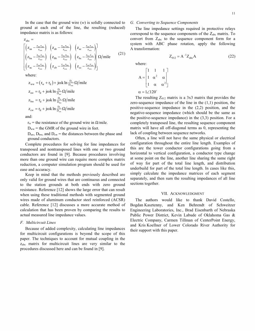
In the case that the ground wire (w) is solidly connected to ground at each end of the line, the resulting (reduced) impedance matrix is as follows:

( ) ( ) ( )( ) ( ) ( )( ) ( ) ( )

aw aw aw bw aw cw

ww ww ww

bw aw bw bw bw cw

ww ww ww

cw aw cw bw cw cw

ww ww ww

abc

z z z z z zaa ab acz z z

z z z z z zba bb bcz z z

z z z z z zac cb ccz z z

z

z z z

z z z mile

z z z

=

− − − − − − Ω

− − −

(21)

where:

( ) e

ww

e

aw

e

bw

e

cw

Dww w d D

Daw d D

Dbw d D

Dcw d D

z r r j k ln mile

z r j k ln mile

z r j k ln mile

z r j k ln mile

= + + ω Ω

= + ω Ω

= + ω Ω

= + ω Ω

and: rw = the resistance of the ground wire in Ω/mile. Dww = the GMR of the ground wire in feet. Daw, Dbw, and Dcw = the distances between the phase and ground conductors.

Complete procedures for solving for line impedances for transposed and nontransposed lines with one or two ground conductors are found in [9]. Because procedures involving more than one ground wire can require more complex matrix reduction, a computer simulation program should be used for ease and accuracy.

Keep in mind that the methods previously described are only valid for ground wires that are continuous and connected to the station grounds at both ends with zero ground resistance. Reference [12] shows the large error that can result when using these traditional methods with segmented ground wires made of aluminum conductor steel reinforced (ACSR) cable. Reference [12] discusses a more accurate method of calculation that has been proven by comparing the results to actual measured line impedance values.

F. Multicircuit Lines Because of added complexity, calculating line impedances

for multicircuit configurations is beyond the scope of this paper. The techniques to account for mutual coupling in the zabc matrix for multicircuit lines are very similar to the procedures discussed here and can be found in [9].

G. Converting to Sequence Components The line impedance settings required in protective relays

correspond to the sequence components of the Zabc matrix. To convert from Zabc to the sequence component form for a system with ABC phase rotation, apply the following A transformation:

–1012 abcZ A Z A= (22)

where:

2

2

1 1 1

A 1

1

1 120

= α α α α

α = ∠

The resulting Z012 matrix is a 3x3 matrix that provides the zero-sequence impedance of the line in the (1,1) position, the positive-sequence impedance in the (2,2) position, and the negative-sequence impedance (which should be the same as the positive-sequence impedance) in the (3,3) position. For a completely transposed line, the resulting sequence component matrix will have all off-diagonal terms as 0, representing the lack of coupling between sequence networks.

Often, a line will not have the same physical or electrical configuration throughout the entire line length. Examples of this are the tower conductor configurations going from a horizontal to vertical configuration, a conductor type change at some point on the line, another line sharing the same right of way for part of the total line length, and distribution underbuild for part of the total line length. In cases like this, simply calculate the impedance matrices of each segment separately, and then sum the resulting impedances of all line sections together.

VII. ACKNOWLEDGMENT The authors would like to thank David Costello,

Bogdan Kasztenny, and Ken Behrendt of Schweitzer Engineering Laboratories, Inc., Brad Eisenbarth of Nebraska Public Power District, Kevin Labude of Oklahoma Gas & Electric Company, Carmen Tillman of CenterPoint Energy, and Kris Koellner of Lower Colorado River Authority for their support with this paper.

12

VIII. REFERENCES [1] E&S Grounding Solutions, “What Is Soil Resistivity Testing?”

Available: http://www.esgroundingsolutions.com/about-electrical-grounding/what-is-soil-resistivity-testing.php.

[2] United States Federal Communications Commission Encyclopedia, “M3 Map of Effective Ground Conductivity in the United States (A Wall Sized Map), for AM Broadcast Stations.” Available: http://www.fcc.gov /encyclopedia/m3-map-effective-ground-conductivity-united-states-wall -sized-map-am-broadcast-stations.

[3] C. F. Wagner and R. D. Evans, Symmetrical Components. McGraw-Hill, New York, 1933.

[4] D. A. Tziouvaras, J. Roberts, and G. Benmouyal, “New Multi-Ended Fault Location Design for Two- or Three-Terminal Lines,” proceedings of the 7th International Conference on Developments in Power System Protection, Amsterdam, Netherlands, April 2001.

[5] Alstom Grid, Network Protection & Automation Guide, May 2011. Available: http://alstom.com.

[6] H. J. Altuve Ferrer and E. O. Schweitzer, III (eds.), Modern Solutions for Protection, Control, and Monitoring of Electric Power Systems. Schweitzer Engineering Laboratories, Inc., Pullman, WA, 2010.

[7] J. L. Blackburn and T. J. Domin, Protective Relaying: Principles and Applications, 3rd ed. CRC Press, Boca Raton, FL, 2007.

[8] S. E. Zocholl, “Symmetrical Components: Line Transposition.” Available: http://www.selinc.com.

[9] P. M. Anderson, Analysis of Faulted Power Systems. Wiley-IEEE, New York, 1995.

[10] J. J. Grainger and W. D. Stevenson, Jr., Power System Analysis. McGraw-Hill, 1994.

[11] J. R. Carson, “Wave Propagation in Overhead Wires With Ground Return,” The Bell System Technical Journal, Vol. V, pp. 539–554, 1926.

[12] B. Thapar, V. Gerez, and A. Balakrishnan, “Zero-Sequence Impedance of Overhead Transmission Lines With Discontinuous Ground Wire,” proceedings of the 22nd Annual North American Power Symposium, Auburn, AL, October 1990.

IX. BIOGRAPHIES Ariana Amberg earned her BSEE, magna cum laude, from St. Mary’s University in 2007. She graduated with a Masters of Engineering in Electrical Engineering from Texas A&M University in 2009, specializing in power systems. Ariana joined Schweitzer Engineering Laboratories, Inc. in 2009 as an associate field application engineer. She has been an IEEE member for 9 years.

Alex Rangel received a BSEE and an MSE from The University of Texas at Austin in 2009 and 2011, respectively. In January 2011, Alex joined Schweitzer Engineering Laboratories, Inc., where he works as an associate field application engineer. Alex is currently an IEEE member.

Greg Smelich received a BS in Mathematical Science from Montana Tech of the University of Montana in 2008. After graduating, he decided to pursue an MS in Electrical Engineering from Montana Tech and earned his degree in 2011. Shortly after, Greg joined Schweitzer Engineering Laboratories, Inc. as an associate field application engineer. Greg is currently an IEEE member.

Previously presented at the 2012 Texas A&M Conference for Protective Relay Engineers. © 2012, 2016 IEEE – All rights reserved.

20160425 • TP6539-01