1

Validating the Bland-Altman Method of Agreement

Ryan Fernandez, University of Nevada-Las Vegas

George Fernandez, University of Nevada-Reno ABSTRACT Bland-Altman’s analysis and plot are the most common methods used to assess the relative agreement between two analytical methods that measure the continuous variables measured on the same scale. Many agreement studies have shown that using the t-test or the Pearson’s product-moment correlation is flawed when measuring the agreement or detecting the bias. Bland-Altman proposed graphical techniques for analyzing method comparison and validation studies and many articles advocating their approach or variations of it have since appeared in many journals. The basic concept of Bland-Altman’s approach is the visualization of the difference of the measurements made by the two methods, then plotting the differences (diff) or the bias (Y-axis) versus the mean (mean) of the two readings (X-axis). In addition, additional reference lines such as the zero bias line and 95% upper (0 + 1.96 Sdiff) and 95% lower (0 - 1.96 Sdiff) are also overlaid on the same scatter plot. When there is no systematic bias, it is easy to verify from the plot if the differences are symmetrical around zero. If there is no relationship between the differences and the averages, the agreement between the two methods may be summarized using the means and standard deviations test methods. Bland-Altman’s plots have become an essential requirement in validity or method-comparison studies and Bland-Altman’s original paper has been cited over more than 11500 occasions—compelling evidence of its importance in medical research. However, some recent reports discussed the flaws of the Bland-Altman’s graphical methods and advocate the use of regression approach especially when the bias distribution shows heterogeneous bias distribution. Therefore, we are proposing a robust enhanced Bland-Altman’s analysis which combines a superior graphical display of bias distribution supplemented with a regression analysis between the diff and the standard measurement. The primary objective of this poster presentation is using advanced SAS statistical and graphical procedures to demonstrate our enhanced features of robust Bland-Altman’s analysis and compare its performances with the original Bland-Altman’s method using six diverse types of simulated data sets. INTRODUCTION Medical researchers often need to compare two methods of measurements, such as blood pressure levels, blood glucose, weights of newborn infants, or a new method (test method) with an established one (standard method) to determine whether these two methods can be used interchangeably or the new method can replace the established measurement. A chemist may wish to see whether a new, inexpensive and quick method produces measurements that are clinically in close agreement with those from an established method. For comparison of one method with another, Bland and Altman (1986) proposed a method consisting of two measurements on a group of subjects, and then plotting the difference scores against the mean for each subject. Bland-Altman proposed their plot to discourage researchers away from the misuse of applications of the correlation coefficient between these two measurements as a measure of validity. Problems with using the correlation analysis and t-test have been noted by Altman and Bland (1983) and Bland and Altman (1986). The problem with the correlation

2

coefficient is that the two measures might be highly correlated, yet there could be substantial differences in the two measurements across their range of values. The basic concept of Bland-Altman’s approach is the visualization of the difference of the measurements made by the two methods, then plotting the differences (diff) or the bias (Y-axis) versus the mean (mean) of the two readings (X-axis). Additional reference lines, zero bias line, 95% upper (0 + 1.96 Sdiff) and 95% lower (0 - 1.96 Sdiff) are also overlaid on the same scatter plot. When there is no systematic bias, it is easy to see the differences are symmetrical around zero. If there is no relationship between the diff and the mean, the agreement between the two methods may be summarized using the means and standard deviations of the differences. Since then there has been an increasing use of the Bland–Altman plot over the years, from 8% in 1995 to 14% in 1996, and 31–36% in more recent years (Myles PS and Cui J. (2007)). However, Hopkins (2000) discussed the flaws of the Bland-Altman’s graphical methods and advocates the use of regression approach especially when there is heterogeneous bias distribution. He claimed that measures of bias are only one aspect of a validity study and equal importance must be given to the nature of the random error in measurements provided by the instrument. The magnitude of the error is usually calculated as the standard error of the bias estimate and the researcher should examine the scatter for heteroscedasticity (non-uniformity) when there is more scatter at the high end of predicted values. In these cases, Bland-Altman’s recommend the use of a log transformation of the data points whereas Hopkins (2000) proposed the use of simple linear regression between the two measurements and a test for heteroscedasticity. In this paper, we are proposing methods to enhance the Bland-Altman’s graphical display and modify the regression approach by regressing the diff on standard measurement and propose methods to test the significance of the intercept and the slope in the presence of heteroscedasticity. Then using six diverse types of simulated data sets, the proposed enhanced features of robust Bland-Altman’s analysis will be compared with the performances of the original Bland-Altman’s method. METHODS a) Original Bland-Altman’s graphical method using the SAS SGPLOT in version 9.2 (See Figures 1-6). Please see the SAS code used in Appendix 1:

• Create a scatter plot between the difference of the readings made by the two methods, then plot the differences (diff) or the bias (Y-axis) versus the mean (mean) of the two readings (X-axis).

• Add additional reference lines such as the zero bias line, 95% upper (0 + 1.96 Sdiff) and 95% lower (0 - 1.96 Sdiff ) to the same scatter plot.

When there is no systematic bias, it is easy to verify from the plot if the differences are symmetrical around zero. b) Proposed enhanced Bland-Altman’s graphical method using the SAS SGPLOT in version 9.2 (See Figures 1-6):

• Substitute a needle plot for the scatter plot and create a plot between the difference of the readings made by the two methods (diff) or the bias (Y-axis) versus the actual or standard measurement in the X-axis (mean of the two measurements is substituted by the accurate or standard measurements in the enhanced plot) .

3

• Add the regression line, its 95% confidence interval band and an additional zero bias reference lines to the enhanced plot.

• If the regression line and the zero bias line falls within the 95% CLM band then conclude that the bias trend is statistically NOT different from the zero bias line.

• If the regression line falls above the 95% CLM band and the slope of this regression line is horizontal then conclude that a significant homogeneous positive bias exists for the new method or the test method when compared with the standard method.

• If the regression line falls below the 95% CLM band and the slope of this regression line is horizontal then conclude that a significant homogeneous negative bias exists for the new method or the test method when compared with the standard method.

• If the regression line slope is significant with a positive or negative slope and intersect the 95% confidence band, then conclude that significant nonsystematic heterogeneous bias exists. However, verify that this bias is not caused by the heteroscedastic error distribution by performing test for significant heteroscedasticity.

c) Robust heteroscedastic consistent regression model (PROC REG):

• Fit the following regression model: diffi = β0 + β1 xi + εi where o Diffi = (New or test measurement – standard or the actual measurement) o β0 = Y-intercept , a measure of systematic positive or negative bias o β1 = Slope, a measure of non systematic heterogeneous bias o xi = standard or the actual measurement o εi = independent normally distributed homogeneous random error

• Test the error distribution for homoscedasticity by using the PROC REG option SPEC. • If the homoscedasticity assumption is satisfied then test the following hypotheses:

o H0: β0 = 0 o H0: β1 = 0

• If the homoscedasticity assumption is NOT satisfied then test the following hypotheses using ACOV option in the MODEL statement. ACOV option displays the heteroscedastic -consistent covariance matrix and adds heteroscedastic -consistent standard errors, also known as White standard errors, to the parameter estimates table (PROC REG, SAS Online documentation).

o H0: β0 = 0 o H0: β1 = 0

• Interpretation: o H0: β0 = 0 and β1 = 0 are not rejected: No bias. Validate the new method o H0: β0 = 0 is rejected but β1 = 0 not Rejected; Positive are negative

homogeneous bias. o H0: β0 = 0 and β1 = 0 are rejected: Significant bias exists. Presence of

significant heterogeneous bias is confirmed. RESULTS AND DISCUSSION The method agreement results between the standard Bland-Altman and proposed enhanced robust Bland-Altman method were compared using the following six diverse simulated studies. The results of the six comparative studies are presented below: Study1: Simulated data with zero bias

4

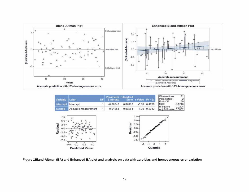
Actual or the known standard measurement = (From 5 to 40 by an increment of 0.5) + (random error (e1) = (1.5*rannor(0)+0)) Test method value = From 5 to 40 by an increment of 0.5) + (random error (e2)= (2.5*rannor(0)+0)) The results of the standard Bland-Altman analysis and proposed enhanced robust Bland-Altman method are presented in Appendix2-Figure1. When there is no systematic bias with an estimate of 10% average error, the standard Bland-Altman plot clearly showed the random nature of the bias around the zero bias line. Except for three data points, all the bias values (diff) fell within 95% of the prediction limits. The enhanced Bland-Altman plot also revealed the same results in the enhanced display. In addition, the enhanced Bland-Altman plot revealed the following additional features:

o The needle plot clearly shows the direction of the bias more effectively than the scatter plot display.

o Both the regression and the zero bias lines fell within the 95% confidence band indicating that both the intercept and the slope of the regression line are not significantly different from zero.

The results of the robust regression analysis from SAS PROC REG revealed the following: o The random distribution of the residuals in the residual plot clearly showed that the

homoscedasticity assumption is not violated. o The normal probability plot showed that the residual has a normal distribution o Both β0 and β1 are not statistically different from zero ( P-value > 0.05) confirming the

findings from the graphical results This study confirms that when there is no systematic bias in method agreement, the standard Bland-Altman plot and the enhanced robust Bland-Altman were comparable and were effective, making the correct conclusion. Study2: Simulated data with 16% positive bias with no heteroscedasticity Actual or the known standard measurement = (From 5 to 40 by an increment of 0.5) + (random error (e1)= (1.5*rannor(0)+0)) Test method value =( (From 5 to 40 by an increment of 0.5) + (positive bias=4) ) + (random error (e2)= (2.5*rannor(0)+0)) The results of the standard Bland-Altman analysis and the proposed enhanced robust Bland-Altman method are presented in Appendix2 –Figure2. When there is a positive systematic bias (16%) with an estimate of 10% average error, the standard Bland-Altman plot clearly showed a random nature of the spread with significant positive bias (majority of the bias points were positive). More than 20% of the biased points fell outside the upper 95% prediction limits. The enhanced Bland-Altman plot also revealed the same results in the enhanced display. In addition, the enhanced Bland-Altman plot revealed the following additional features:

o The needle plot clearly shows the positive bias more effectively than the scatter plot display.

o The zero bias lines fell below the lower 95% confidence band indicating that the intercept is significantly greater than zero.

5

o The estimated slope of the regression line is zero because the regression line fell within the 95% confidence interval band.

The results of the robust regression analysis from SAS PROC REG revealed the following: o The random distribution of the residuals in the residual plot clearly showed that the

homoscedasticity assumption is not violated. o The normal probability plot showed that the residual has a normal distribution o Only β1 is not statistically different from zero (P-value > 0.05) where as the estimate of

β0 was significantly different and confirms the findings from the graphical results of the known simulated data.

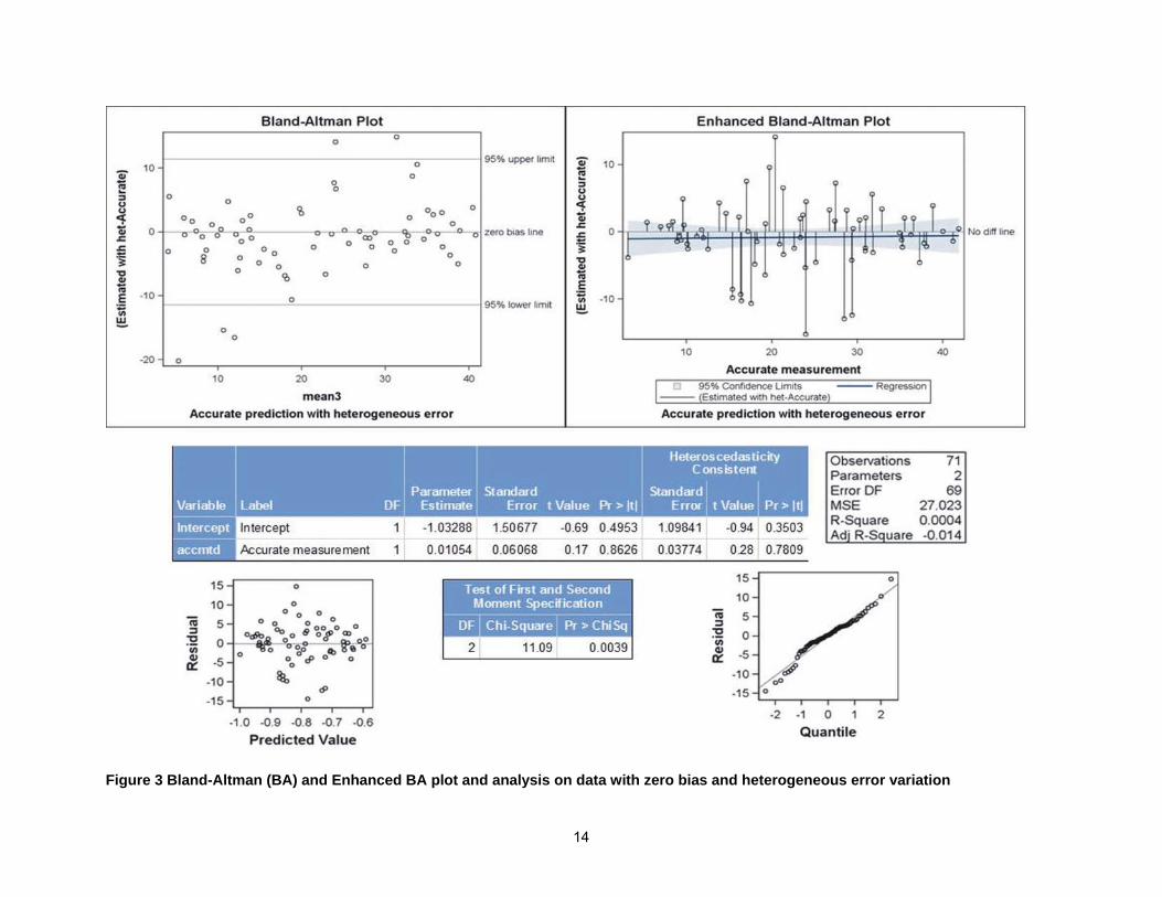
This study confirms that when there is homogeneous systematic bias in method agreement, the standard Bland-Altman plot and the enhanced robust Bland-Altman were effective in making correct inferences and detecting the positive bias. However, enhanced robust Bland-Altman method revealed additional features of the positive bias and offers additional capabilities to detect the nature of the bias. Study3: Simulated data with zero bias and significant heteroscedasticity Actual or the known standard measurement = (From 5 to 40 by an increment of 0.5) + (random error (e1) = (1.5*rannor(0)+0)) Test method value: Test measurement less than 15 or greater than 30: measurement value + (random error (e2)= (2.5*rannor(0)+0)) Test measurement between 15 to 30 with 3 times larger error: measurement value + (random error (e2) = 3*(2.5*rannor(0)+0)) The results if the standard Bland-Altman analysis and proposed enhanced robust Bland-Altman method is presented in Appendix2–Figure3. When there is NO systematic bias with significant heteroscedastic error, the standard Bland-Altman plot clearly showed a random nature of the spread with zero bias. Only less than 5% of the points fell outside the 95% prediction limits. Thus the standard Bland-Altman analysis failed to detect the heteroscedastic error distribution. The enhanced Bland-Altman plot also revealed the zero bias in the enhanced display. In addition, the enhanced Bland-Altman plot revealed the following additional features:

o The needle plot clearly shows the nature of heteroscedastic error (larger degree of error in the mid range of test values) more effectively than the scatter plot display.

o The zero bias lines and the regression lines fell within the 95% confidence band confirming that both the intercept and the slopes are NOT significantly different from zero, confirming the zero bias in the estimation.

The results of the robust regression analysis from SAS PROC REG revealed the following: o The diamond shaped distribution of the residuals in the residual plot clearly showed that

the homoscedasticity assumption is violated significantly. o The normal probability plot showed that the residuals have a normal distribution o Chi-square test clearly showed significant heteroscedasticity indicating that standard t-

tests for regression parameter estimates are not valid. However, valid hypothesis tests can be performed using heteroscedasticity -consistent standard errors.

o Both β0 and β1 were not statistically different from zero ( P-value > 0.05) based on heteroscedasticity -consistent standard errors which confirm the findings from the graphical results of the known simulated data.

6

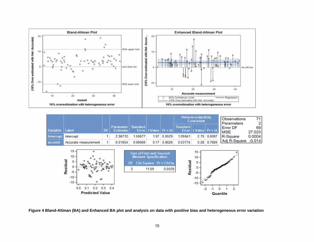
This study confirms that when there is NO systematic bias in method agreement, the standard Bland-Altman plot and the enhanced robust Bland-Altman were effective in making correct inferences about zero bias. However, standard Bland-Altman method failed to detect the presence of heteroscedasticity whereas enhanced robust Bland-Altman method revealed heteroscedasticity. Study4: Simulated data with 16% positive bias with significant heteroscedasticity Actual or the known standard measurement = (From 5 to 40 by an increment of 0.5) + (random error (e1) = (1.5*rannor(0)+0)) Test method value: Test measurement less than 15 or greater than 30: (measurement value+ positive bias:4) + (random error (e2)= (2.5*rannor(0)+0)) Test measurement between 15 to 30 with 3 times larger error: (measurement value+ positive bias=4) + (random error (e2) = 3*(2.5*rannor(0)+0)) The results of the standard Bland-Altman analysis and proposed enhanced robust Bland-Altman method are presented in Appendix2–Figure4. When there is positive systematic bias with significant heteroscedastic error, the standard Bland-Altman plot showed a random nature of the spread with positive bias. The presence of heteroscedasticity was not clearly evident in the standard Bland-Altman plot. Only less than 5% of the points fell below the zero line. Thus the standard Bland-Altman analysis failed to detect the heteroscedastic error distribution. The enhanced Bland-Altman plot revealed the positive bias and the heterogeneous error in the enhanced display. In addition, the enhanced Bland-Altman plot revealed the following additional features:

o The needle plot clearly shows the nature of heteroscedastic error (larger degree of error in the mid range of test values) more effectively than the scatter plot display.

o The zero bias line falls outside the 95% confidence band indicating the presence of significant positive intercept, which validates the presence of positive bias.

o The regression line fell within the 95% confidence band confirming that the regression slope is NOT significantly different from zero, confirming a homogeneous bias in the estimation.

The results of the robust regression analysis from SAS PROC REG revealed the following:

o The diamond shaped distribution of the residuals in the residual plot clearly showed that the homoscedasticity assumption is violated significantly.

o The normal probability plot showed that the residual has a normal distribution o Chi-square test clearly showed significant heteroscedasticity indicating that standard t-

tests for regression parameter estimates are not valid. However, valid hypothesis tests can be performed using heteroscedasticity -consistent standard errors.

o The regression slope β1 is not statistically different from zero (P-value > 0.05) based on heteroscedasticity -consistent standard errors confirm the findings from the graphical results of the known simulated data.

o The intercept β0 is statistically different from zero (P-value < 0.05) based on heteroscedasticity -consistent standard errors which confirm the findings from the graphical results of the known simulated data

This study confirms that when there is systematic bias in method agreement, the standard Bland-Altman plot and the enhanced robust Bland-Altman were effective in making correct inferences about zero bias. However, standard Bland-Altman method failed to detect the

7

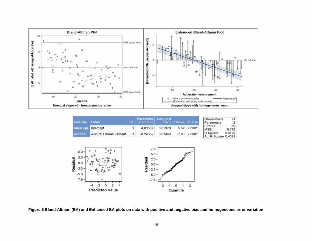
presence of heteroscedasticity whereas enhanced robust Bland-Altman method revealed heteroscedasticity. Study5: Simulated data with heterogeneous bias and non- significant heteroscedasticity Actual or the known standard measurement = (From 5 to 40 by an increment of 0.5) + (random error (e1)= (1.5*rannor(0)+0)) Test method value: Test measurement less than 20: (measurement value + 3) + (random error (e2) = (2.5*rannor(0)+0)) Test measurement greater than or equal 20: (measurement value – 3) + (random error (e2) = (2.5*rannor(0)+0)) The results of the standard Bland-Altman analysis and proposed enhanced robust Bland-Altman method is presented in Appendix2–Figure5. When there is heterogeneous bias with no heteroscedastic error, the standard Bland-Altman plot failed to prominently show the nature of the positive and the negative bias in the scatter plot. Also only less than 5% of the points fell outside the 95% prediction limits. Thus the standard Bland-Altman analysis failed to detect the heterogeneous bias. However, the enhanced Bland-Altman plot clearly revealed the heterogeneous bias. In addition, the enhanced Bland-Altman plot revealed the following additional features:

o The needle plot clearly shows the nature of both positive and the negative more effectively than the scatter plot display.

o The zero bias lines intersects the 95% confidence band confirming that both the intercept and the slopes are significantly different from zero which confirms the presence of heterogeneous bias in the estimation.

The results of the robust regression analysis from SAS PROC REG revealed the following:

o The quadratic nature of the distribution of the residuals in the residual plot clearly showed the heterogeneous nature of the bias. But, as expected there is no evidence of heteroscadastic error.

o The normal probability plot showed that the residual has a normal distribution o Both β0 and β1 were statistically different from zero ( P-value < 0.05) based on the

standard regression output which confirms the findings from the graphical results of the known simulated data.

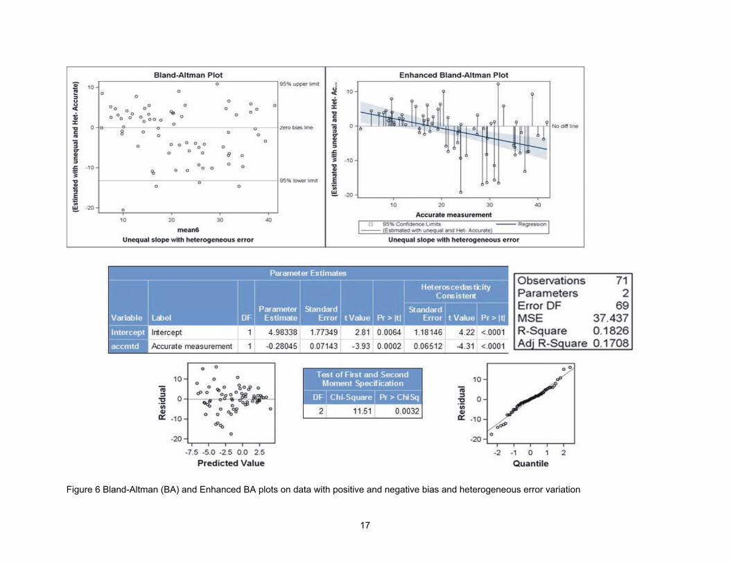
This study confirms that when there is systematic bias in method agreement, the standard Bland-Altman plot failed to detect heterogeneous bias pattern. However, the enhanced robust Bland-Altman analysis is very effective in making correct inferences about heterogeneous bias. Study6: Simulated data with heterogeneous bias and significant heteroscedasticity Actual or the known standard measurement = (From 5 to 40 by an increment of 0.5) + (random error (e1)= (1.5*rannor(0)+0)) Test method value: Test measurement less than 20: (measurement value + 3) + (random error (e2) = (2.5*rannor(0)+0)) Test measurement greater than or equal 20: (measurement value – 4) + (random error (e2) = 3*(2.5*rannor(0)+0)) The results of the standard Bland-Altman analysis and the proposed enhanced robust Bland-Altman method are presented in Appendix2–Figure6.

8

When there is heterogeneous bias with significant heteroscadastic error, the standard Bland-Altman plot showed a random nature of the spread and failed to detect the heterogeneous bias with significant heteroscadastic error. The presence of heteroscadasticity was not clearly evident in the standard Bland-Altman plot. Thus the standard Bland-Altman analysis failed to detect the heterogeneous error and heteroscadastic error distribution. The enhanced Bland-Altman plot clearly revealed the heterogeneous bias and the heterogeneous error in the enhanced display. In addition, the enhanced Bland-Altman plot revealed the following additional features:

o The needle plot clearly shows the nature of heteroscadastic error (larger degree of error in the mid and the upper range of test values) more effectively than the scatter plot display.

o The zero bias line intersects the 95% confidence band indicating the presence of significant regression slope which validates the presence of heterogeneous bias.

The results of the robust regression analysis from SAS PROC REG revealed the following:

o The diamond shaped distribution of the residuals in the residual plot clearly showed that the homoscedasticity assumption is violated significantly.

o The normal probability plot showed that the residual has a normal distribution o Chi-square test clearly showed significant heteroscedasticity indicating that standard t-

tests for regression parameter estimates are not valid. However, valid hypothesis tests can be performed using heteroscedasticity -consistent standard errors.

o The intercept β0 and the regression slope β1 were statistically different from zero ( P-value < 0.05) based on heteroscedasticity-consistent standard errors which confirm the findings from the graphical results of the known simulated data.

This study confirms that when there is heterogeneous bias with significant heteroscadastic error, the standard Bland-Altman plot failed to detect both problems. However, enhanced robust Bland-Altman method clearly revealed heterogeneous bias with significant heteroscadastic error. SUMMARY The results based on these six simulated studies reveled that the standard Bland-Altman plot was effective only in the presence of zero or homogeneous positive error. When the nature of the bias is heterogeneous and the error distribution is heteroscedastic, the standard Bland-Altman plot was ineffective. However, the proposed enhanced Bland-Altman plot and the heteroscedasticity -consistent regression analysis method clearly detected zero bias, homogeneous and heterogeneous bias and the presence of homoscedastic and heteroscedastic error. Version 9.2 SAS codes for performing the data simulation, standard and enhanced Bland-Altman plot, and heteroscedasticity -consistent regression analysis are given in the Appendix1. REFERENCES 1. Bland JM, Altman DG (1986). Statistical methods for assessing agreement between two methods of clinical measurement. Lancet i, 307-310 2 Bland JM, Altman DG. Measuring agreement in method comparison studies. Stat Methods Med Res 1999; 8: 135–60

9

3. Bland JM, Altman DG (2003). Applying the right statistics: analyses of measurement studies. Ultrasound in Obstetrics and Gynecology 22, 85-93 4. Hopkins WG (2000). Measures of reliability in sports medicine and science. Sports Medicine 30, 1-15 5. Katy D. Fierens C Sto¨ckl D. Linda M. Thienpont (2002) Application of the Bland–Altman Plot for Interpretation of Method-Comparison Studies: A Critical Investigation of Its Practice Clinical Chemistry 48, No. 5 6. Ludbrook J (2002). Statistical techniques for comparing measurers and methods of measurement: a critical review. Clinical and Experimental Pharmacology and Physiology 29, 527–536 7. Myles PS and Cui J. (2007) Using the Bland–Altman method to measure agreement with repeated measures British Journal of Anesthesia Editorial I 309-11 CONTACT INFORMATION Your comments are greatly appreciated and encouraged. Contact the authors at: Ryan D Fernandez University Nevada – Las Vegas Phone: 775-830-0687 Email: ryadynfer@yahoo.com George Fernandez University of Nevada, Reno Work Phone: (775) 784-4206 Email: gcjf@unr.edu SAS and all other SAS Institute Inc. product or service names are registered trademarks or trademarks of SAS Institute Inc. in the USA and other countries. ® indicates USA registration. Other brand and product names are trademarks of their respective companies.

10

APPENDIX1 SAS CODE data fatp; do fat= 5 to 40 by 0.5; e1=(1.5*rannor(0)+0); e2=(2.5*rannor(0)+0); accmtd=fat+e1; estmtd=fat+e2; estmtd2=(fat+4)+ e2; if accmtd< 15 or fat >30 then estmtd3=fat+e2; else estmtd3= fat+(3*e2); if accmtd< 15 or fat >30 then estmtd4=(fat+4)+e2; else estmtd4= (fat+4)+(3*e2); if accmtd< 20 then estmtd5=(fat+3)+e2; else estmtd5= (fat-3)+e2; if accmtd< 20 then estmtd6=(fat+3)+e2; else estmtd6= (fat-4)+(3*e2); diff=estmtd-accmtd; diff2=estmtd2-accmtd; diff3=estmtd3-accmtd; diff4=estmtd4-accmtd; diff5=estmtd5-accmtd; diff6=estmtd6-accmtd; mean = (estmtd+accmtd)/2; mean2= (estmtd2+accmtd)/2; mean3= (estmtd3+accmtd)/2; mean4= (estmtd4+accmtd)/2; mean5= (estmtd5+accmtd)/2; mean6= (estmtd6+accmtd)/2; label accmtd ='Accurate measurement' estmtd ='Estimated measurement' estmtd2 = '16% Over-estimated measurement' estmtd3 ='Estimated measurement with Hetero' estmtd4 = '16% Over-estimated measurement with Heteros' estmtd5 ='Estimated measurement with unequal slope' estmtd6 = ' Estimated measurement with unequal slope and Heteros' diff= '(Estimated-Accurate)' diff2 ='(16% Over-estimated- Accurate)' diff3= '(Estimated with het-Accurate)' diff4 ='(16% Over-estimated with Het- Accurate)' diff5= '(Estimated with unequal-Accurate)' diff6 ='(Estimated with unequal and Het- Accurate)' ; output; end; ods listing close; ods rtf file='c:\temp\blandaltman.rtf' style=sasweb; ods graphics on; proc means data=fatp noprint; var diff;

11

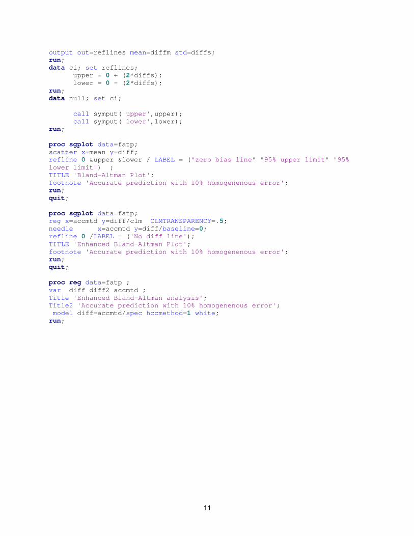
output out=reflines mean=diffm std=diffs; run; data ci; set reflines; upper = 0 + (2*diffs); lower = 0 - (2*diffs); run; data null; set ci; call symput('upper',upper); call symput('lower',lower); run; proc sgplot data=fatp; scatter x=mean y=diff; refline 0 &upper &lower / LABEL = ("zero bias line" "95% upper limit" "95% lower limit") ; TITLE 'Bland-Altman Plot'; footnote 'Accurate prediction with 10% homogenenous error'; run; quit; proc sgplot data=fatp; reg x=accmtd y=diff/clm CLMTRANSPARENCY=.5; needle x=accmtd y=diff/baseline=0; refline 0 /LABEL = ('No diff line'); TITLE 'Enhanced Bland-Altman Plot'; footnote 'Accurate prediction with 10% homogenenous error'; run; quit; proc reg data=fatp ; var diff diff2 accmtd ; Title 'Enhanced Bland-Altman analysis'; Title2 'Accurate prediction with 10% homogenenous error'; model diff=accmtd/spec hccmethod=1 white; run;

12

Figure 1Bland-Altman (BA) and Enhanced BA plot and analysis on data with zero bias and homogeneous error variation

13

Figure2. Bland-Altman (BA) and Enhanced BA plot and analysis on data with positive bias and homogeneous error variation

14

Figure 3 Bland-Altman (BA) and Enhanced BA plot and analysis on data with zero bias and heterogeneous error variation

15

Figure 4 Bland-Altman (BA) and Enhanced BA plot and analysis on data with positive bias and heterogeneous error variation

16

Figure 5 Bland-Altman (BA) and Enhanced BA plots on data with positive and negative bias and homogeneous error variation

17

Figure 6 Bland-Altman (BA) and Enhanced BA plots on data with positive and negative bias and heterogeneous error variation