Vacuum Stability in Supersymmetric Effective Theories · Riassunto I principali argomenti trattati...
156
POUR L'OBTENTION DU GRADE DE DOCTEUR ÈS SCIENCES acceptée sur proposition du jury: Prof. M. Q. Tran, président du jury Prof. C. Scrucca, directeur de thèse Prof. G. Dall'Agata, rapporteur Prof. J.-P. Derendinger, rapporteur Prof. R. Rattazzi, rapporteur Vacuum Stability in Supersymmetric Effective Theories THÈSE N O 5192 (2011) ÉCOLE POLYTECHNIQUE FÉDÉRALE DE LAUSANNE PRÉSENTÉE LE 18 NOVEMBRE 2011 À LA FACULTÉ SCIENCES DE BASE GROUPE SCRUCCA PROGRAMME DOCTORAL EN PHYSIQUE Suisse 2011 PAR Leonardo BRIZI
Transcript of Vacuum Stability in Supersymmetric Effective Theories · Riassunto I principali argomenti trattati...
POUR L'OBTENTION DU GRADE DE DOCTEUR ÈS SCIENCES
acceptée sur proposition du jury:
Prof. M. Q. Tran, président du juryProf. C. Scrucca, directeur de thèse
Prof. G. Dall'Agata, rapporteur Prof. J.-P. Derendinger, rapporteur
Prof. R. Rattazzi, rapporteur
Vacuum Stability in Supersymmetric Effective Theories
THÈSE NO 5192 (2011)
ÉCOLE POLYTECHNIQUE FÉDÉRALE DE LAUSANNE
PRÉSENTÉE LE 18 NOvEMBRE 2011
À LA FACULTÉ SCIENCES DE BASEGROUPE SCRUCCA
PROGRAMME DOCTORAL EN PHYSIQUE
Suisse2011
PAR
Leonardo BRIzI

Abstract
The main topics discussed in this thesis are supersymmetric low-energy effective theo-
ries and metastability conditions in generic non-renormalizable models with global and
local supersymmetry.
In the first part we discuss the conditions under which the low-energy expansion
in space-time derivatives preserves supersymmetry implying that heavy multiplets can
be more efficiently integrated out directly at the superfield level. These conditions
translate into the requirements that also fermions and auxiliary fields should be small
compared to the heavy mass scale. They apply not only to the matter sector, but
also to the gravitational one if present, and imply in that case that the gravitino mass
should be small. We finally give a simple prescription to integrate out heavy chiral and
vector superfields consisting respectively in imposing stationarity of the superpotential
and of the Kahler potential; the procedure holds in the same form both for global and
local supersymmetry.
In the second part we study general criteria for the existence of metastable vacua
which break global supersymmetry in models with local gauge symmetries. In par-
ticular we present a strategy to define an absolute upper bound on the mass of the
lightest scalar field which depends on the geometrical properties of the Kahler target
manifold. This bound can be saturated by properly tuning the superpotential and its
positivity therefore represents a necessary and sufficient condition for the existence of
metastable vacua. It is derived by looking at the subspace of all those directions in
field space for which an arbitrary supersymmetric mass term is not allowed and scalar
masses are controlled by supersymmetry-breaking splitting effects. This subspace in-
cludes not only the direction of supersymmetry breaking, but also the directions of
gauge symmetry breaking and the lightest scalar is in general a linear combination of
fields spanning all these directions. Our purpose is to show that the largest value for
the lightest mass is in general achieved when the lightest scalar is a combination of the
Goldstone and the Goldstino partners.
We conclude by computing the effects induced by the integration of heavy multiplets
on the light masses. In particular we focus on the sGoldstino partners and we show that
heavy chiral multiplets induce a negative level-repulsion effect that tends to compromise
vacuum stability, whereas heavy vector multiplets in general induce a positive-definite
contribution.
Our results find application in the context of string-inspired supergravity models,
where metastability conditions can be used to discriminate among different compactifi-
cation scenarios and supersymmetric effective theories can be used to face the problem
of moduli stabilization.
Keywords: Standard Model, Supersymmetry Breaking, Hidden Sector, Moduli,
Supergravity, Effective Field Theories, Vacuum Stability.

Riassunto
I principali argomenti trattati in questo lavoro di tesi sono le teorie supersimmetriche
effettive di bassa energia e le condizioni di metastabilita nell’ambito di generici modelli
non rinormalizzabili con supersimmetria globale e locale.
Inizialmente discutiamo le condizioni per cui la supersimmetria viene preservata
dallo sviluppo in derivate, in modo tale che i multipletti pesanti possano essere integrati
via direttamente in supercampi. Le condizioni si traducono nel richiedere che anche i
bilineari fermionici ed i campi ausiliari siano piccoli rispetto alla massa dei multipletti
pesanti. Le stesse condizioni si applicano sia ai campi di materia che a quelli del
settore gravitazionale, qualora esso sia presente; in quest’ultimo caso pero, e necessario
richiedere che anche la massa del gravitino sia piccola. Concludiamo definendo una
procedura per integrare via i multipletti chirali e vettoriali che consiste nell’imporre
rispettivamente la stazionarieta del superpotenziale e del potenziale di Kahler; la stessa
procedura vale sia nel caso di supersimmetria rigida che di supergravita.
Nella seconda parte studiamo alcuni criteri generali per l’esistenza di vuoti metasta-
bili che rompono la supersimmetria in modelli con simmetrie di gauge. In particolare,
proponiamo una strategia per definire un limite superiore assoluto per la massa dello
scalare piu leggero che dipende dalle proprieta geometriche della varieta di Kahler.
Questo limite puo essere saturato fissando opportunamente i parametri del superpoten-
ziale e pertanto, il fatto che esso sia positivo, costituisce una condizione necessaria e
sufficiente per la metastabilita. Il limite e ottenuto considerando le direzioni nello spazio
dei campi che non ammettono una massa supersimmetrica arbitrariamente grande e tali
che le masse degli scalari associati siano interamente controllate da effetti di rottura di
supersimmetria. Questo sottospazio include non soltanto la direzione di rottura della
supersimmetria, ma anche le direzioni di rottura delle simmetrie di gauge e, in generale,
lo scalare piu leggero risulta essere una combinazione lineare di queste direzioni. Il nos-
tro obbiettivo e di mostrare che il valore massimo per la massa piu leggera si ottiene in
generale quando lo scalare piu leggero e una combinazione dei partner scalari associati
al Goldstino e ai Goldstones.
Concludiamo studiando gli effetti indotti dall’integrazione di multipletti pesanti
sulle masse di quelli leggeri; in particolare ci concentriamo sulla massa dei partner
scalari del Goldstino e mostriamo che i multipletti chirali pesanti contribuiscono con
un effetto negativo di level-repulsion che tende a compromettere la metastabilita mentre
i multipletti vettoriali pesanti inducono in generale un contributo positivo.
I nostri risultati possono trovare applicazione nell’ambito dei modelli di supergravita
derivanti dalla Teoria delle Stringhe, dove le condizioni di mestabilita possono essere
usate per discriminare tra differenti scenari di compattificazione mentre le teorie effet-
tive possono essere usate per affrontare il problema della stabilizzazione dei moduli.
Keywords: Modello Standard, Rottura di Supersimmetria, Supergravita, Moduli,
Settore Nascosto, Teorie di Campo Effettive, Stabilita del Vuoto.


A Eleonora, Francesca e Valentina

Contents
Introduction 1
1 Supersymmetry and Supergravity 7
1.1 Effective Field Theories and Natural Hierarchies . . . . . . . . . . . . . 8
1.2 SUSY as a Solution to the Hierarchy Problem and Beyond . . . . . . . 11
1.3 Global Supersymmetry . . . . . . . . . . . . . . . . . . . . . . . . . . . 14
1.3.1 Models with only Chiral Multiplets . . . . . . . . . . . . . . . . 14
1.3.2 Models with Chiral and Vector Multiplets . . . . . . . . . . . . 17
1.4 Local Supersymmetry . . . . . . . . . . . . . . . . . . . . . . . . . . . . 24
1.4.1 Models with only Chiral Multiplets . . . . . . . . . . . . . . . . 24
1.4.2 Models with Chiral and Vector Multiplets . . . . . . . . . . . . 33
2 Supersymmetry Breaking 39
2.1 The Minimal Supersymmetric Standard Model . . . . . . . . . . . . . . 39
2.2 The Hidden Sector Paradigm and Soft SUSY Breaking . . . . . . . . . 42
2.2.1 Gravity Mediation . . . . . . . . . . . . . . . . . . . . . . . . . 44
2.2.2 Gauge Mediation . . . . . . . . . . . . . . . . . . . . . . . . . . 47
2.3 Hidden Sector in String-Inspired Models . . . . . . . . . . . . . . . . . 49
3 Supersymmetric Effective Field Theories 53
3.1 Integrating Out Heavy Fields: General Setup . . . . . . . . . . . . . . . 54
3.1.1 The Derivative Expansion . . . . . . . . . . . . . . . . . . . . . 56
3.2 Integrating Out Heavy Chiral Multiplets in Global SUSY . . . . . . . . 57
3.3 Integrating Out Heavy Chiral Multiplets in Supergravity . . . . . . . . 62
3.4 Integrating Out Heavy Vector Multiplets in Global SUSY . . . . . . . . 70
3.5 Integrating Out Heavy Vector Multiplets in Supergravity . . . . . . . . 75
3.6 Summary . . . . . . . . . . . . . . . . . . . . . . . . . . . . . . . . . . 76
4 Vacuum Stability and Bound on the Lightest Scalar 79
4.1 General Criteria for Metastability . . . . . . . . . . . . . . . . . . . . . 79
ix
x Contents
4.2 Structure of the Scalar Mass Matrix . . . . . . . . . . . . . . . . . . . . 82
4.3 Bound on the Lightest Scalar Mass . . . . . . . . . . . . . . . . . . . . 88
4.4 Renormalizable Gauge Theories . . . . . . . . . . . . . . . . . . . . . . 91
4.5 Non-linear Gauged Sigma Models . . . . . . . . . . . . . . . . . . . . . 94
4.6 Explicit Examples with Constant Curvature . . . . . . . . . . . . . . . 96
4.6.1 Flat Kahler Potential and Linear Isometry . . . . . . . . . . . . 97
4.6.2 Logarithmic Kahler Potential and Shift-Isometry . . . . . . . . 98
4.6.3 Logarithmic Kahler Potential and Linear Isometry . . . . . . . . 99
4.7 Summary . . . . . . . . . . . . . . . . . . . . . . . . . . . . . . . . . . 102
5 Effects of Heavy Multiplets on Vacuum Stability 105
5.1 General Considerations . . . . . . . . . . . . . . . . . . . . . . . . . . . 106
5.2 Effect of Heavy Chiral Multiplets . . . . . . . . . . . . . . . . . . . . . 107
5.2.1 Component Approach . . . . . . . . . . . . . . . . . . . . . . . 110
5.2.2 Superfield Approach . . . . . . . . . . . . . . . . . . . . . . . . 113
5.3 Effect of Heavy Vector Multiplets . . . . . . . . . . . . . . . . . . . . . 114
5.3.1 Component Approach . . . . . . . . . . . . . . . . . . . . . . . 116
5.3.2 Superfield Approach . . . . . . . . . . . . . . . . . . . . . . . . 118
5.4 Summary . . . . . . . . . . . . . . . . . . . . . . . . . . . . . . . . . . 119
Conclusions 123
Acknowledgements 127
A Numerical Optimization of the Local Superpotential 129
Bibliography 140
“But precisely to the hero
is beauty
the hardest thing of all.
Unattainable is beauty
by all ardent wills.”
Friedrich Nietzsche
Thus Spake Zarathustra.

Introduction
We are entering a very exciting era for high energy physics! In November 2009 the
Large Hadron Collider (LHC) at CERN in Geneva officially became the most powerful
particle accelerator in the world. The energy scale which is going to be systematically
explored by the LHC is the teraelectronvolt (TeV= 1012 eV) which is 11 orders of
magnitude larger than the energy required to ionize a hydrogen atom. At these energies,
physicists are going to probe the fundamental interactions between matter constituents
up to distances of the order of 100 zeptometers (10−19 m) which is 9 orders of magnitude
smaller than the typical atomic size! The theoretical framework describing physics at
such scales is the quantum theory of fields which combines in a unified formalism the
two most important physical theories of the 20th century namely Special Relativity and
Quantum Mechanics.
The Standard Model is the universally accepted quantum theory of the fundamental
particles and forces; it describes the physics of three fermionic generations of quarks
and leptons and their interactions mediated by the exchange of gauge bosons. The
Standard Model has been tested with extremely high accuracy up to energies of the
order of 102 GeV and no significant deviations have been observed so far between
theoretical predictions and experimental data. Despite this enormous success, one
fundamental building block of the Standard Model is still missing: the Higgs boson.
This particle is the elementary excitation of a fundamental field (the Higgs field) which
is expected to trigger the spontaneous breaking of the electroweak symmetry and to
give mass to both the gauge bosons of weak interactions and to the matter fermions. On
top of that, the Higgs boson is a crucial ingredient of the Standard Model also because
it ensures the unitarity of the scattering amplitudes of longitudinally polarized gauge
bosons at energies of the order of 1 TeV. If the Higgs boson is not found in the near
future, some new mechanism is expected to show up at the TeV scale, and this is
exactly the energy range which is going to be extensively investigated by the LHC.
Besides the obvious interest for the Higgs sector, there exist other important mo-
tivations to expect very exciting physics at the TeV scale; this is because, even if the
Higgs boson is discovered at the LHC, there are still several reasons to consider the
Standard Model a partly unsatisfactory theory. The first problem we can mention is
the fact that the Standard Model depends on too many free parameters (precisely 19)
which must be fixed by experimental measurements; in particular the theory does not
predict the values of the quark and lepton masses and there is no fundamental ex-
1
2 Introduction
planation for the different hierarchies among them. Another important aspect is that
the Standard Model describes only three of the four fundamental interactions so far
discovered in nature namely the electromagnetic, the strong and the weak interactions.
The inclusion of gravity in this scheme presents some important difficulties. In par-
ticular it implies that the Standard Model is not a truly fundamental theory but just
a low-energy effective description which is valid only up to the energy scale at which
gravity becomes as strong as the other interactions. The energy scale at which this is
expected to happen is the Planck scale which is of the order of 1028 eV, 16 orders of
magnitude larger than the TeV scale! There exist, however, some potential problems in
considering the Standard Model as a low-energy effective theory valid up to the Planck
scale. The major difficulty comes from the fact that the Higgs boson mass receives very
large quantum corrections from the exchange of virtual particles at the quantum level
and these contributions are in general of the order of the Planck mass, which is very
large compared to the expected order of magnitude of the Higgs physical mass. Such a
small value can arise only as a consequence of bizarre cancellations of large unrelated
contributions, achieved by an extremely accurate fine tuning of the parameters of the
theory, and is then very unnatural. This problem associated to the naturalness of the
Higgs mass is known as the hierarchy problem and it is the main theoretical argument
to expect new physics beyond the Standard Model at the TeV scale. Other important
limitations of the Standard Model emerge when we also consider cosmological obser-
vations; indeed the theory does not include a candidate sector for the dark matter
and there is no natural explanation for the small value of the cosmological constant,
introduced in Einstein’s equations of General Relativity to explain the cosmological
expansion of the Universe.
The quest for the high energy completion of the Standard Model and for the fun-
damental theory unifying gravity with the other interactions is the major challenge
of modern high energy physics research. In the construction of realistic models of
physics beyond the Standard Model, theoretical physicists are commonly guided and
inspired, as in the case of the hierarchy problem, by aesthetic criteria like naturalness,
elegance and simplicity; the most successful theories are considered to be those which,
starting from the smallest number of hypotheses or assumptions, succeed in explaining
the greatest number of empirical facts. There is nothing wrong in being inspired by
subjective criteria like beauty or symmetry to formulate physical theories; on the other
hand, the greatest mystery of science is probably the fact that nature seems to follow
exactly the same criteria!
There are essentially two approaches to the study of physics beyond the Standard
Model: on one hand one can try to guess what the theory describing all the interac-
tions in an unified way at the Planck scale is and identify the low-energy features of
the theory using consistency arguments. On the other hand one can look at the low-
energy experimental facts which are not naturally explained in the Standard Model
and search for a more natural explanation for them. It is very remarkable that these
two approaches appear to converge in the same direction defining a special ingredi-
Introduction 3
ent which is expected to characterize physics beyond the Standard Model: the idea
of supersymmetry (SUSY). From the low-energy phenomenological perspective, super-
symmetry represents a natural mechanism to explain the small value of the Higgs mass;
the way this is achieved is by postulating the existence of a fundamental symmetry
relating bosons and fermions which automatically enforces the miraculous cancellations
among the large quantum corrections to the Higgs mass. On the other hand, from the
purely theoretical high-energy perspective, supersymmetry appears also to be a neces-
sary ingredient of String Theory, which is the only presently known candidate theory
for a unified fundamental description of all the interactions at the Planck scale.
Despite the enormous appeal of supersymmetry, the construction of realistic super-
symmetric models presents some very non-trivial aspects. The difficulties are associated
to the fact that SUSY cannot exist as an exact symmetry of nature since in that case
it would predict a degenerate spectrum of fermion and boson masses which is not ex-
perimentally observed. On the other hand, if one expects supersymmetry to be the
mechanism responsible for the stabilization of the Higgs mass, it cannot be arbitrarily
broken. Most of the difficulties then arise because it is known from some general sum
rules that the spontaneous breaking of supersymmetry must involve a completely new
sector, called hidden sector, which interacts with the Standard Model particles only
through suppressed interactions and whose physics is a priori completely unknown.
A very common paradigm is to assume that the hidden sector contains the moduli
sector of String Theory. Moduli fields are neutral scalar fields whose vacuum expecta-
tion values determine the geometrical properties of the compactification manifold and
which interact with Standard Model fields only through gravitational interactions sup-
pressed by inverse powers of the Planck mass. The fact that moduli are in general ex-
pected to be stabilized with non-vanishing vacuum expectation values makes them very
natural candidates for triggering the spontaneous breaking of supersymmetry. In this
scenario, gravity is assumed to be the principal mechanism by which supersymmetry-
breaking effects are transmitted to Standard Model superpartners. This suggests that
the most natural theoretical framework to study supersymmetry breaking is actually
supergravity (SUGRA).
In this thesis work we will review and extend some useful tools that can be used
to simplify the study of the moduli sector physics in string-inspired models. There
are two fundamental difficulties that one has to face in this context. The first one
is the fact that there exists a very large variety of models which correspond to dif-
ferent compactification scenarios, but not all of them are expected to give a realistic
description of our universe. The second problem is the fact that for each particular
model there is a proliferation of moduli fields and in general an analytical study of
the full dynamics is totally prohibitive. The first complication requires the study of
some general criteria to efficiently discriminate among different scenarios. As a matter
of fact, the only strong condition one can impose on realistic models is the existence
of (at least) one metastable vacuum which breaks supersymmetry with a small and
positive cosmological constant. Tackling the second difficulty requires the possibility
4 Introduction
of reducing the number of moduli fields that are effectively important in the study of
the low-energy supersymmetry breaking dynamics. This can be done by integrating
out all the heavy moduli that are stabilized with large supersymmetric masses and con-
structing a low-energy effective field theory describing the dynamics of the remaining
light moduli. To summarize, the main objective of this thesis is to develop some useful
strategies to tackle the two problems mentioned above; metastability conditions and
supersymmetric effective theories are the principal instruments we introduce to achieve
our purpose and are the main topics we are going to extensively study in this work.
This thesis is structured as follows. In the first two chapters we review the main
ideas and results in global and local supersymmetry that are relevant for our discus-
sions; the remaining three chapters represent the original core of this work and collect
our main results on supersymmetric effective theories and vacuum stability. To be
more precise, in Chapter 1 we first discuss more in depth the fundamental arguments
motivating the study of supersymmetry; the second part of the chapter is a technical
review of the most general non-renormalizable models containing matter and gauge
fields in SUSY and SUGRA. Particular attention is given to the derivation of the su-
pergravity Lagrangian which, for later convenience, is performed in the superconformal
formalism. In Chapter 2 we discuss in some detail supersymmetry breaking focusing
our attention on the constraints imposed by the supertrace formula and the hidden
sector paradigm; we then present two important transmission mechanisms, namely
gravity and gauge mediation. We conclude by discussing the characteristics of the
hidden sector in string-inspired models and by better defining the problematics which
inspire this work.
Chapter 3 is dedicated to the study of low-energy effective theories and the consis-
tent supersymmetric integration of heavy multiplets in global and local supersymme-
try. This part is based on the results presented in our paper Brizi, Gomez-Reino and
Scrucca, 2009 [1]. Our main contribution relates to the integration of heavy multiplets
in supergravity theories, since the case of rigid supersymmetry has already been ex-
tensively studied in the literature both for chiral and vector multiplets. In the case of
SUGRA we find that one can use the same procedure valid in the rigid case to integrate
out heavy multiplets at the superfield level provided that the mass of the gravitino,
or equivalently the cosmological constant, is small compared to the heavy field mass
scale.
Chapter 4 is devoted to the study of metastability conditions in general non-linear
σ-models including both chiral and vector multiplets. This part is based on the results
presented in our paper Brizi and Scrucca, 2011 [2]. Our main contribution consists in
this case in clarifying the role of Goldstone partners in defining the strongest upper
bound on the mass of the lightest scalar in models in which the superpotential can be
arbitrarily varied while the Kahler potential and the gauged isometries are assumed
to be fixed. This work extends and improves some previous studies in which only
the Goldstino partners were taken into account to define necessary conditions for the
existence of metastable vacua.
Introduction 5
In Chapter 5 we combine the general ideas of the previous two chapters and study
the effects induced by the integration of heavy multiplets on the masses of the light
scalars and on the metastability conditions; this is done in the special case for which all
vector multiplets are heavy and the only potentially dangerous modes are the Goldstino
partners. This part is based on the results presented in our paper Brizi and Scrucca,
2010 [3]. In this chapter we show that the correction to the effective sGoldstino mass
induced by heavy chiral multiplets is always negative and tends to compromise vacuum
metastability, whereas the contribution from heavy vector multiplets is always positive
and tends, on the contrary, to reinforce it.
In the section dedicated to the conclusions we present a detailed summary of the
main results achieved in this thesis and discuss some possible future directions.

6
Chapter 1
Supersymmetry and Supergravity
In this chapter we present a review of the basic ideas and tools in global and local
N = 1 supersymmetry that will be useful for future discussions; in particular we
focus our attention on the class of generic non-renormalizable models called non-linear
σ-models.
In the first part we review the most important arguments singling out supersymme-
try as one of the most fascinating conjectured feature of physics beyond the Standard
Model. We show that there exist several hints, mostly based on phenomenological and
on purely theoretical arguments, which suggest that supersymmetry may play a rele-
vant role in describing physics at the TeV scale and beyond. This first part has the form
of a brief non-technical review of the main motivations for studying supersymmetry.
In the following sections we review in a pragmatic way the structure of non-linear
σ-models both in SUSY and SUGRA, focusing our attention on the derivation of the
scalar potential and the mass matrices. In the rigid case we schematically recall the
derivation of the full Lagrangian and the masses of scalar, spinor and gauge fields; we
will use these expressions to revisit the supertrace formula which imposes strong con-
straints on the possibility of realizing realistic scenarios for supersymmetry breaking.
This part is presented as a brief technical review of the main formulas that we will
need in the following chapters; since this topic is quite standard and well established
we will focus on the main concepts avoiding too many details.
In the case of supergravity theories, we will present in some detail the construction
of the most general Lagrangian. This part is less standard since in the literature there
exist several different approaches to the subject; for this reason we will perform a more
careful and detailed analysis. It turns out that the most suitable framework for our
purposes is the superconformal supergravity formalism. We therefore revisit the main
steps and arguments followed in the construction of the supergravity Lagrangian in this
approach and we recall the expressions of the scalar potential and the scalar masses
which will be extensively used in the following chapters.
7
8 Supersymmetry and Supergravity
1.1 Effective Field Theories and Natural Hierar-
chies
At present time there exist several indications suggesting that supersymmetry [4–6]
should be considered as a plausible guiding principle for physics beyond the Standard
Model [7–9]. Before discussing the main arguments in favor of this hypothesis, let us
first review the modern point of view on the Standard Model and why it is expected
to be an incomplete theory.
The very first consideration we can do is that the Standard Model cannot be a
fundamental theory because it does not include a truly fundamental description of
gravitational interactions at the quantum level. More precisely, the canonical quanti-
zation of General Relativity produces a non-renormalizable quantum field theory with
a dimensionful coupling 1/M2P proportional to the inverse of the Planck mass. From
a modern perspective, the fact the Standard Model plus General Relativity is a non-
renormalizable quantum field theory means that it is an effective description which is
valid only for energies much smaller than the cut-off scale MP at which the effective
coupling E2/M2P becomes of order one. At the Planck scale this picture is expected
to break down and should be replaced by a more fundamental theory which includes
new degrees of freedom. A priori there are no serious motivations to believe that this
ultimate theory is a renormalizable quantum field theory; in fact, most attempts to
construct a truly fundamental quantum theory of gravitational interactions are based
on completely new paradigms (e.g. String Theory). We conclude that renormalizabil-
ity should not be considered as a fundamental principle in quantum field theory model
building; non-renormalizable theories are perfectly fine as long as we consider them as
low energy effective descriptions of more fundamental theories; it is exactly in this sense
that we consider the Standard Model as an incomplete (or not fundamental) theory.
Renormalizable quantum field theories are very peculiar theories; technically renor-
malizability corresponds to the possibility of extrapolating long range physics to small
distances without encountering new degrees of freedom. In this sense renormalizable
quantum field theories can be truly fundamental descriptions of nature. However,
more in general, effective Lagrangians do not contain only renormalizable operators
of dimension di 6 4 but include also a tower of higher-dimensional operators whose
couplings are suppressed by the mass scale Λ at which new physics shows up:
Leff = Ldi64 +∑di>4
λdiOdi
Λdi−4, (1.1)
where Odi are operators of dimension di and λdi are dimensionless couplings; Ldi64 is
the renormalizable Lagrangian. At tree level, the effect of each coupling can be tracked
by simple dimensional analysis; in particular only the dimensionless effective couplings
λdi(E) ∼ λdi (E/Λ)di−4 can enter in the definition of observable amplitudes. This anal-
ysis shows that in the infrared region E Λ only the operators in the renormalizable
Lagrangian are important whereas the contributions coming from the higher dimen-
1.1. Effective Field Theories and Natural Hierarchies 9
sional ones flow to zero. Operators with mass dimension di < 4 are called relevant
since they always give important contributions in the infrared; the ones with di > 4 are
called irrelevant since their effects disappear in the low-energy regime; finally operators
with di = 4 are called marginal and the associated tree -level effects are independent
of the energy scale. Despite the infinite tower of higher-dimensional operators, non-
renormalizable Lagrangians conserve a predictive power. Indeed at each finite order
(E/Λ)n, only a finite number of operators contribute to the amplitudes; this is in fact
not too restrictive since theoretical predictions must be matched with experimental ob-
servations which have finite precision. Quantum corrections introduce some technical
subtleties in this analysis but do not spoil the general picture. This can be seen by
choosing a regularization scheme (such as Dimensional Regularization) which does not
exhibit power-like divergencies; in that case, simple dimensional analysis considerations
hold also true at the quantum level. It is also possible to see that renormalizable La-
grangians are stable under loop corrections in the sense that no new higher-dimensional
operator is generated at the quantum level. On the other hand, if a non-renormalizable
operator is included at tree level, infinitely many higher-dimensional operators are gen-
erated by quantum effects.
The Standard Model, by itself, is a renormalizable theory, and a priori it is thus a
good candidate to be a fundamental theory; however, as we have seen, when gravity
is included this is not true anymore. Actually, even without introducing gravity, there
is no reason to assume that there does not exist any new physical effect arising at
some high energy scale smaller than the Planck mass, since the Standard Model has
been tested only up to energies of order 102 GeV. From a low energy perspective,
what we can do is to experimentally estimate the scale Λ at which new physics can
appear. At present time no significant deviations from Standard Model predictions have
been experimentally observed; moreover the accuracy achieved in past experiments is
sufficiently high to conclude that new physics effects are strongly suppressed and the
new physics scale should be very large. More precisely, we observe for example that
dimension-six four-fermion operators violating baryon number are suppressed by a scale
of order [10]
ΛB/ & 1015 GeV . (1.2)
Other constraints on new physics come from flavor-violating processes and the associ-
ated operator are found to be suppressed by a scale of order [10]
ΛF/ & 106 GeV . (1.3)
Despite the good agreement between Standard Model predictions and observations,
there are still some unsatisfactory aspects of the model which motivate theoretical
particle physicists to expect that some new physics should actually show up at smaller
scales. In particular, some problematic aspects of the Standard Model, as we are going
to see, require a solution in terms of new physics in the TeV region. In the following we
are going to discuss the so called hierarchy problem (or naturalness problem) [11, 12],
which is one of the most significant theoretical drawbacks of the Standard Model. It
10 Supersymmetry and Supergravity
has inspired most of the modern scenarios for physics beyond the Standard Model
and, more relevantly, it is the most important phenomenological motivation to study
supersymmetry.
The hierarchy problem is associated with the theoretical difficulty in explaining in a
natural way the small value of the Higgs mass that is suggested by precision electroweak
measurements [10]:
mh . 150GeV. (1.4)
As we are going to discuss in a moment, this value is very unnatural if the energy
scale Λ associated to the new physics is much larger than the TeV scale. It is worth
to stress that the hierarchy problem is not a theoretical inconsistency of the Standard
Model; it is however a well motived question about the naturalness of one of its pa-
rameters which appears to be unnaturally adjusted. The existence of this fine-tuning
suggests that, very likely, some new underlying mechanism is “conspiring” to produce
such an unexpected value.
The problem consists in the fact that a large hierarchy between the Higgs mass
and the physical cut-off is not automatically stable under quantum corrections; more
precisely, loop corrections to the Higgs mass are quadratic in Λ:
(m2h)eff = m2
h(Λ) + cΛ2 + ... (1.5)
and tend to destroy the hierarchy unless the tree-level mass is unnaturally tuned. The
amount of the necessary fine tuning increases with the scale at which new physics effects
become sizable and for Λ 'MP it turns out to be a formidable task to naturally explain
such a huge hierarchy between the Higgs mass and the Planck scale.
It is natural to expect that if a particle has a mass which is much smaller than Λ
there should exist a symmetry (at least an approximate one) under which the mass
term is forbidden; in this case we say that the mass is “protected” by a symmetry 1.
In ordinary quantum field theory, many examples of naturally small masses protected
by symmetries are known. For example, the photon is naturally massless since gauge
invariance prevents quantum corrections from generating a mass term for it. Similarly,
chiral symmetry forbids a mass term for Dirac fermions implying that quantum cor-
rections are not proportional to the large cut-off but to the fermion mass itself. Scalar
particles, on the other hand, can be naturally light if they are (pseudo) Goldstone
bosons of a spontaneously broken (approximate) global symmetry. In this case shift
symmetry forbids a mass term and the scalar field has only derivative couplings.
In the Standard Model, none of the above mentioned mechanisms prevents large
quantum corrections to the tree-level mass of the Higgs scalar. In absence of any
symmetry principle we then expect mh ' Λ.
1This naturalness criterium has been rigorously formulated by ’t Hooft [13].
1.2. SUSY as a Solution to the Hierarchy Problem and Beyond 11
1.2 SUSY as a Solution to the Hierarchy Problem
and Beyond
As we anticipated, supersymmetry offers a natural explanation for the small value
of the Higgs mass; this is achieved by protecting the mass of scalar fields by a new
(unconventional) symmetry relating bosons and fermions. Supersymmetry is not an
ordinary symmetry in the sense that its algebra is a graded Lie algebra; besides the
ordinary (commuting) bosonic generators of the internal and Poincare symmetries, it
contains anticommuting fermionic generators Q implementing transformations of boson
into fermions and vice-versa; schematically:
Q |B〉 = |F 〉 , Q |F 〉 = |B〉 . (1.6)
Global supersymmetry requires that particles belonging to the same supermulti-
plet are degenerate in mass; this implies that the same chiral symmetry which forbids
fermion mass terms protects also scalar masses from large quantum corrections. Tech-
nically, the way in which this is achieved is through the cancellation of the dangerous
loop diagrams among superpartners of different spins; such cancellations are enforced
by the peculiar structure of the dimensionless couplings required by supersymmetry
invariance. More precisely, the large quadratic quantum corrections to the Higgs mass
associated to loops of heavy fermions (the top or some new heavy particle) are cancelled
by loop diagrams of the corresponding scalar superpartners:
∆m2h ∝
1
8π2(λφ − |λψ|2 ) Λ2 + ... ; (1.7)
the cancellation is possible thanks to the special relations between the couplings which
hold in supersymmetry and which guarantee that:
λφ = |λψ|2 . (1.8)
However, as explained more extensively in Chapter 2, supersymmetry cannot be an
exact symmetry of nature and must be broken by some mechanism in order to explain
the non-observation of the predicted degeneracy between Standard Model particles and
superparticles. On the other hand, if supersymmetry is the mechanism responsible for
the stabilization of the electroweak scale, it cannot be broken in an arbitrary way.
In the next chapter we will discuss in some detail soft supersymmetry breaking; here
we limit ourselves to mention the fact that supersymmetry breaking terms should not
spoil the relation between dimensionless couplings which ensure the cancellation of
the dangerous quantum corrections to all orders in perturbation theory. This means
that supersymmetry-breaking terms should be relevant operators with dimensionful
couplings. If we call msoft the scale associated to these operators we have that:
∆m2h ∝ m2
soft , (1.9)
12 Supersymmetry and Supergravity
which implies that msoft cannot exceed too much the TeV range to avoid fine-tuning
problems.
Supersymmetry is not the only mechanism which has been investigated to solve the
hierarchy problem. A more conventional mechanism to generate naturally large hierar-
chies is by dimensional transmutation of dimensionless couplings in asymptotically-free
non-Abelian gauge theories (as for example in QCD). The basic idea is to start with
a theory which has no dimensionful couplings; the fundamental scale ΛIR of the the-
ory is then dynamically generated at the quantum level by the anomalous breaking of
the scale invariance. More precisely, the low energy scale ΛIR at which the coupling
becomes of order one and perturbation theory breaks down is given by:
ΛIR
Λ= e
−8π2
b g20 , (1.10)
where g0 denotes the value of the gauge coupling at the large ultra-violet cut-off scale Λ.
At the scale ΛIR, gauge interactions become strong and the creation of fermion conden-
sates 〈ψψ〉 with a scale of order ΛIR can take place. An example of such condensates
in QCD are pions. These mesons are three pseudo-Goldstone bosons associated with
chiral symmetry breaking and have masses which are much smaller than the other
hadronic resonances. The important aspect is that the presence of light scalar mesons
does not give rise to any fine-tuning problem since a large hierarchy between ΛIR and
Λ can be achieved in a natural way without need to tune the coupling g0 with an ex-
tremely high accuracy. Models based on this mechanism are called Technicolor [14, 15];
in these models the Higgs is not a fundamental particle but (effectively) a composite
one, similarly to the case of pions in QCD. In this case however the scale at which the
postulated new interaction becomes strong is much larger than the one associated to
strong interactions (ΛQCD ' 200 MeV) and it is of the order of ΛTC ' 500 GeV. With-
out entering any further into the details of these models, we just mention the fact that
the minimal realization of the Technicolor scenario as a scaled version of QCD does
not work; qualitatively speaking, this is because the six-dimensional operators which
generate quark masses is as relevant as the dangerous higher-dimensional (4-quarks)
operators which produce anomalous flavor changing effects.
We conclude this general and not completely exhaustive discussion 2 on the possible
solutions to the hierarchy problem by mentioning a third class of models which assumes
the existence of large extra dimensions [17]. In this scenario the large hierarchy between
the electroweak scale and the Planck scale is completely removed and gravity becomes
strong at the TeV scale, which is assumed to be the only fundamental scale in the theory.
The observed weakness of gravity at distances larger than the millimeter range is due to
the existence of (at least 2) new compact spatial dimensions which are large compared
to the weak scale; Standard Model particles are supposed to be constrained by some
mechanism to live on a four-dimensional manifold whereas gravity can also propagate
over all the extra dimensions. The phenomenological signature of this scenario is the
2For a more complete review at the same level of details see for example [16].
1.2. SUSY as a Solution to the Hierarchy Problem and Beyond 13
appearance of quantum gravity effects at the TeV scale.
Even though we introduced supersymmetry as a very plausible solution to the
hierarchy problem, this is not the only reason to be interested in it. There exist
in fact at least two other remarkable indications which suggest that supersymmetry is
likely to play a relevant role for physics beyond the Standard Model. These are indirect
evidences coming from theoretical speculations about physics at very high energy scales
(much larger than the TeV scale). In this context, the main paradigm guiding the
theoretical investigation is the idea of unification of gauge interactions (Grand Unified
Theories, GUT) and, at higher energy, the unification of all the interactions, including
gravity (String Theories). It is a remarkable fact that, in both cases, supersymmetry
seems to emerge as the fundamental ingredient which must be taken into account. In
the case of GUTs [18], the unification of gauge couplings within the Standard Model
is inconsistent with the observations at LEP (see for instance [19]). This rules out any
minimal GUTs which break directly to the Standard Model gauge group with only
ordinary matter field content. The inclusion of additional particles or intermediate
steps in the symmetry breaking pattern may improve the situation but a large amount
of model dependence is unavoidably introduced in this way. On the contrary, in the
case of supersymmetric GUTs case (see [20] for an extended review), unification is
achieved with a very good precision within the minimal supersymmetric extension of
the Standard Model (see Chapter 2); the grand unification scale is predicted to be
at MG ' 1016 GeV, quite close to MP which is considered as the scale at which also
gravity is expected to unify with all the other interactions.
As we anticipated, supersymmetry is also intimately connected to String Theory
[21, 22]; in this context its role seems to be even more fundamental. More precisely, any
of the five known String Theories admits an effective low-energy description in terms of
a supergravity theory in 10 space-time dimension; moreover some of these supergravity
models can be obtained from dimensional reduction of N = 1 supergravity in 11
dimensions, which is supposed to be the low energy limit of an even more fundamental
theory called M-theory. Most of these topics go beyond the principal objectives of
this thesis and they will not be developed any further in the following. However, we
think it is worth to mention them to stress again the fact that the hierarchy problem
should not be considered as the unique motivation to study supersymmetric models;
the most relevant hints indicating supersymmetry as a very appealing ingredient of
physics beyond the Standard Model come not only from bottom-up analyses based on
phenomenological observations but also from more abstract theoretical considerations
in a top-bottom approach.
With these considerations, we conclude this non-technical review of the main ar-
guments motivating the study of supersymmetry; in the remaining sections of this
chapter we will review in some detail the more technical aspects of globally and locally
supersymmetric models.
14 Supersymmetry and Supergravity
1.3 Global Supersymmetry
To start we review some basic ingredients of supersymmetric quantum field theories.
The most compact and efficient framework to represent the supersymmetry algebra on
fields is the formalism of superfields in superspace; for an exhaustive introduction to the
subject see [23–26]. The concept of superspace emerges very naturally in the context of
the usual coset construction as an extension of Minkowski space-time and requires the
introduction of four extra fermionic coordinates (Grassmannian coordinates) θα and
θα. The fermionic nature of these new coordinates implies that any series expansion of
superfields along these extra directions will involve a finite (small) number of ordinary
fields. The basic building blocks used to construct supersymmetric Lagrangians are
chiral superfields and vector superfields which contain respectively matter and gauge
fields, as well as their superpartners and auxiliary fields. Chiral superfields have the
following content in terms of ordinary fields 3:
Φ(x, θ, θ) =φ(x) + i θσµθ ∂µφ(x) +1
4θ2θ2φ(x)
+√
2 θψ(x)− i√2θ2 ∂µψ(x)σµθ + θ2 F (x)
(1.11)
and satisfy the supersymmetric covariant constraint DαΦ = 0, where Dα is the super-
covariant derivative. Vector superfields are given by:
V (x, θ, θ) = −θσµθ Aµ(x) + i θ2 θλ(x)− i θ2 θλ(x) +1
2θ2θ2D(x) (1.12)
and satisfy the reality condition V = V †. In fact the expression (1.12) is not the most
general definition and is obtained from the general expression of the vector superfield
by gauge fixing to zero two scalars (C and N) and one spinor (ξα) corresponding
respectively to the θ0, θ2 and θα components; this gauge choice is known as the Wess-
Zumino gauge. The superfield formalism is very practical to construct supersymmetric
Lagrangians since the tensor product of representations of the SUSY algebra (supermul-
tiplets) simply reduces to the product of superfields; supersymmetric invariant actions
can then be constructed by properly integrating arbitrary functions of superfields over
the whole superspace.
1.3.1 Models with only Chiral Multiplets
In this section we recall the structure and properties of non-linear σ-models containing
only chiral superfields [27, 28]; we restrict ourselves to models which contain the min-
imal number of space time derivatives, which means two derivatives acting on scalar
fields, one derivative acting on fermion fields and no derivatives acting on auxiliary
fields. This assumption corresponds to require that each field propagates the minimal
3In this work we adopt the same conventions as [25].
1.3. Global Supersymmetry 15
amount of degrees of freedom (d.o.f.’s), which means two for each complex scalar, two
for each Weyl fermion and zero for auxiliary fields. The most general Lagrangian that
satisfies these properties is parametrized by two functions, the Kahler potential K(Φ, Φ)
and the holomorphic superpotential W (Φ), and can be expressed in the compact form:
L =
∫d4θ K(Φ, Φ) +
∫d2θW (Φ) + h.c. . (1.13)
The requirement of minimal number of space-time derivatives implies that K and
W cannot depend on supersymmetric covariant derivatives Dα. Indeed, suppose for
example that W depends also on the chiral superfield
D2Φ = −4 F − 4√
2 iθσµ∂µψ − 4φ θ2 ; (1.14)
in this case it is easy to verify that the Lagrangian contains terms which are second
order in space-time derivatives acting on the spinor fields and are controlled by second
derivatives of superpotential.4
The situation is even worse if we suppose that also K depends on the same chiral
superfields D2Φ; in this case the Lagrangian contains also terms with higher derivatives
acting on scalar fields which are controlled by second derivatives of the Kahler potential.
On top of that, also the auxiliary fields F i get kinetic terms and become dynamical in
order to compensate for the fact that spinor fields are now propagating more degrees
of freedom.
The off-shell Lagrangian in component fields is easily found to be:
L = − gi ∂µφi∂µφ − i gi ψσµ(∂µψ
i + Γikl ∂µφkψl)
+ gi FiF +
[F i (Wi −
1
2gi Γ
klψkψ l) + h.c.
]−[ 1
2Wij ψ
iψj + h.c.]
+1
4gi,kl ψ
iψk ψψ l
(1.15)
where gi and Γijk are respectively the Kahler metric and the Levi-Civita connection of
the Kahler manifold associated to the target space spanned by the scalar fields. Notice
that we adopt the short notation in which the derivatives with respect to chiral and
antichiral superfields are denoted by lower indices i and ı which are raised through the
inverse of the Kahler metric.
The Lagrangian is invariant under the action of SUSY transformations on compo-
nent fields:
δφi =√
2 ε ψi , (1.16)
δψi =√
2 ε F i + i√
2σµε ∂µφi , (1.17)
δF i = i√
2 ε σµ∂µψi. (1.18)
4 Note that a superpotential linear in D2Φ of the form W (Φ) = f(Φ) + g(Φ) D2Φ is perfectly fine;however we can rewrite the second term as a total D2 derivative and interpret it as a correction tothe Kahler potential K ′(Φ, Φ) ≡ K(Φ, Φ) + Φ g(Φ) + Φ g(Φ).
16 Supersymmetry and Supergravity
A remarkable property of the Lagrangian (1.15) is that it is not only of leading order in
space-time derivatives, as expected by construction, but also quadratic in the auxiliary
fields F i and in fermion-bilinears ψiψj; this is again a simple consequence of requiring
that the Kahler potential and the superpotential do not depend on supersymmetric
covariant derivatives Dα. From this analysis we learn a very important lesson that
will be useful for future discussions on supersymmetric low energy-effective theories:
supersymmetric models with a limited number of space-time derivatives contain limited
powers of auxiliary fields and fermion bilinears.
The on-shell Lagrangian can be obtained by solving the algebraic equations of
motion of the auxiliary fields F i, which give:
F i = −gi W +1
2Γijk ψ
jψk . (1.19)
Substituting back this relation into L we finally obtain:
L = − gi ∂µφi∂µφ − igi ψiσµ(∂µψ
+ Γmn ∂µφmψn
)+
1
4Rikl ψ
iψkψψ l
− 1
2∇iWj ψ
iψj + h.c.− VS ,(1.20)
where VS is the scalar potential which has the form:
VS = giWiW . (1.21)
A vacuum is defined by constant values of the scalars φi and vanishing values of
the fermions ψi, such that VS is stationary; the stationarity condition then implies:
∇iWj Fj = 0 . (1.22)
The masses for the scalar and fermion fields describing fluctuations around the vacuum
are then found to be given by:
(m20)i = ∇iWk∇W
k −Rikl FkF l , (1.23)
(m20)ij = −∇i∇jWk F
k , (1.24)
and
(m1/2)ij = ∇iWj . (1.25)
From the expressions of the SUSY transformations discussed above, we see that the
vacuum is invariant and supersymmetry is preserved as long as all the auxiliary fields
get vanishing vacuum expectation values (v.e.v’s). On the contrary supersymmetry is
broken whenever one of the auxiliary fields F i is non-vanishing on the vacuum and in
this case the only non-vanishing SUSY variation is: δψi =√
2 ε 〈F i〉. The direction
〈F i〉 in field space is special. For fermions it defines at any stationary point the spinor
field
η =√
2 〈Fi〉ψi , (1.26)
1.3. Global Supersymmetry 17
which transforms inhomogeneously and can then be identified with the Goldstino field
associated to the spontaneous breaking of supersymmetry. As expected, we can easily
verify that the Goldstino has a vanishing mass mη = 0 by using the stationarity
condition (1.22) and the expression of the fermion mass matrix (1.25). For scalar
fields, the direction 〈F i〉 defines instead the supersymmetric partner of the Goldstino,
the sGoldstino
ϕ =√
2 〈Fi〉φi, (1.27)
which transforms under SUSY as δϕ =√
2 ε η. The complex sGoldstino field describes
two real scalar fields whose masses are entirely controlled by supersymmetry breaking
effects; we will see in the following chapters that these special modes play an important
role in discussing the stability properties of the scalar potential.
We conclude this section by recalling the expression of the supertrace of the tree
level mass matrices defined as [29, 30]:
sTr[m2] ≡ Tr[m20]− 2 Tr[m2
1/2] = 2Ri FiF . (1.28)
This formula and its generalization to include vector multiplets (see next section) will
be used in Chapter 2 to review the main obstructions in constructing realistic models
in which supersymmetry is spontaneously broken within the minimal supersymmetric
extension of the Standard Model.
1.3.2 Models with Chiral and Vector Multiplets
In this section we generalize the previous model to include also vector superfields V a
associated to gauge symmetries [31, 32]. We proceed by first considering a model with
only chiral superfields which is invariant under some group G of global symmetries; note
that a group transformation is a symmetry of the action only if it leaves the Kahler
metric invariant or, in other words, if it is an isometry of the Kahler manifold. The
generators of such isometries are holomorphic Killing vectors Xa(Φ) ≡ X ia ∂i and, at
the infinitesimal level, a generic transformation can be written in terms of some real
parameters λa: δ = λa (X ia ∂i + X ı
a ∂ı). It is important to note that the Killing vectors
are not restricted to be linear functions of the superfields; this is because, in general,
at any arbitrary point of the scalar manifold, only the the stabilizer subgroup of Gadmits a linear realization [33] whereas generic group transformations may act non-
linearly on a subset of fields (on the Goldstone bosons for example). Under isometry
transformations, the Kahler potential is demanded to be invariant at least up to a
Kahler transformation: δK = λa [ pa(Φi) + pa(Φ
ı) ]; this implies that:
X iaKi + X ı
aKı = pa(Φi) + pa(Φ
ı) . (1.29)
By taking two sequential covariant derivatives of this expression we obtain Killing’s
equations, which express the invariance of the Kahler metric under Lie dragging:
∇iXa +∇Xai = 0 . (1.30)
18 Supersymmetry and Supergravity
The next step to construct a gauge invariant non-linear σ-model consists, as usual,
in promoting the global symmetry to a local one. First of all we need to promote
each constant parameters λa to be a function of the superspace coordinates (xµ, θ, θ);
more precisely, in order to preserve the chiral nature of matter superfields under gauge
transformations, each group parameter must be promoted to a chiral superfield Λa,
which implies that the gauge group must be complexified. Moreover, we need to intro-
duce a vector superfield V a for each group generator and to require that they properly
transform under gauge transformations in order to make the action invariant under
local symmetry transformations. The Kahler potential must be generalized to include
a dependence on vector fields and it must be invariant under gauge transformation, at
least up to a Kahler transformation:
δK(Φ, Φ, V ) = Λa pa(Φ) + Λa pa(Φ) . (1.31)
Gauge transformations must form a Lie group with an algebra defined by some structure
constants f cab :
[Xa, Xb] = −f cab Xc , (1.32)
and the action of gauge transformation on fields at leading order in Λa is:
δΦi = ΛaX ia(Φ) , (1.33)
δV a = − i2
(Λa − Λa) +
1
2f abc
(Λb + Λb)V c +O(V 2) . (1.34)
When the symmetry is linearly realized these expressions reduce to ordinary gauge
transformations with X ia(Φ) = −i (TaΦ)i, where the generators Ta satisfy the Lie alge-
bra [Ta, Tb] = i f cab Tc; note that the transformation laws for V a do not depend on the
way the symmetry is realized on the chiral fields (whether linearly on non-linearly).
The most general non-renormalizable Lagrangian with leading number of derivatives
is given by:
L =
∫d4θ[K(Φ, Φ, V )
]+
∫d2θ[W (Φ) +
1
4Hab(Φ)W aαW b
α
]+ h.c. , (1.35)
where, in addition to the standard potentials K and W we introduced a holomorphic
gauge kinetic function Hab multiplying the kinetic term of gauge fields; for simplic-
ity we also exclude Fayet-Iliopoulos terms since such terms are not guaranteed to be
compatible with gravitational interactions.
To write down the previous Lagrangian in terms of ordinary fields, it is useful to
fix the Wess-Zumino gauge. In this gauge we can expand K in powers of V and use
the fact that V 3 = 0:
K(Φ, Φ, V ) = K(Φ, Φ) +Ka(Φ, Φ)V a +1
2Kab(Φ, Φ)V aV b . (1.36)
The functions Ka and Kab are not arbitrary and are constrained by gauge invariance to
be functions of the holomorphic Killing vectors. To derive Ka we can use the relation
(1.31) at leading order in Λa evaluated in V a = 0 and we obtain:
Ka = −2iX iaKi + 2i pa . (1.37)
1.3. Global Supersymmetry 19
Taking one derivative of the previous expression with respect to anti-chiral superfields,
we obtain:
X ia =
i
2giKa ; (1.38)
this expression shows that −12Ka can be identified with the Killing potentials for the
Killing vectors X ia. To obtain Kab we can use the fact that the imaginary part of (1.37)
is actually approximately satisfied also for V a 6= 0 up to the second order:
X iaKi − X
aK − iKa = pa − pa +O(V 2) . (1.39)
By taking a derivative of this equation with respect to vector superfields and evaluating
it at V a = 0 we finally obtain:
Kab = 4 giXi(aX
b) . (1.40)
Another important relation can be obtained by imposing the gauge invariance of the
superpotential:
X iaWi = 0 . (1.41)
Gauge invariance of the gauge kinetic Lagrangian implies that the variation of the
gauge kinetic function must cancel the variation of W aα transforming in the adjoint.
This implies that:
X iaHbci = −2f d
a(b Hc)d . (1.42)
Finally an important relation can be obtained by exploiting the equivariance condition
(1.32) on the Killing vectors, which guarantees that the Killing potentials can be chosen
in the adjoint representation, so that:
giXi[aX
b] =
i
4f cab Kc . (1.43)
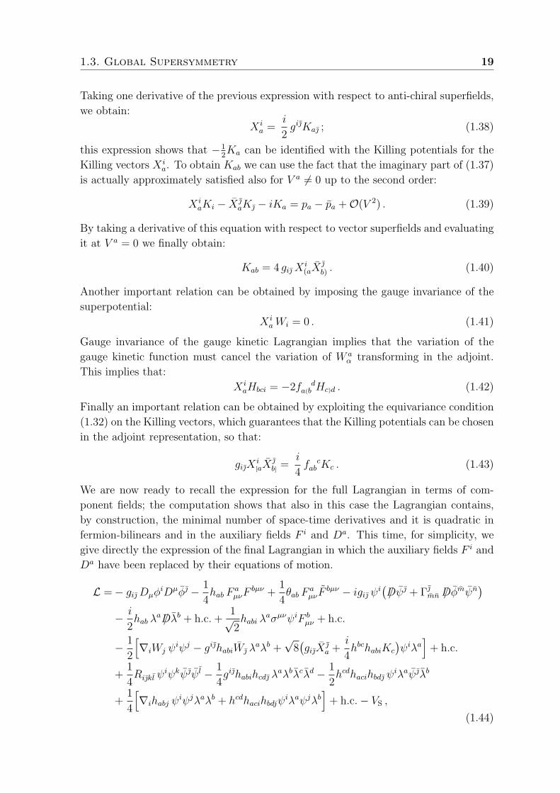
We are now ready to recall the expression for the full Lagrangian in terms of com-
ponent fields; the computation shows that also in this case the Lagrangian contains,
by construction, the minimal number of space-time derivatives and it is quadratic in
fermion-bilinears and in the auxiliary fields F i and Da. This time, for simplicity, we
give directly the expression of the final Lagrangian in which the auxiliary fields F i and
Da have been replaced by their equations of motion.
L =− giDµφiDµφ − 1
4hab F
aµνF
bµν +1
4θab F
aµνF
bµν − igi ψi(D/ ψ + ΓmnD/ φ
mψn)
− i
2hab λ
aD/ λb + h.c.+1√2habi λ
aσµνψiF bµν + h.c.
− 1
2
[∇iWj ψ
iψj − gihabiW λaλb +
√8(giX
a +
i
4hbchabiKc
)ψiλa
]+ h.c.
+1
4Rikl ψ
iψkψψ l − 1
4gihabihcd λ
aλbλcλd − 1
2hcdhacihbd ψ
iλaψλb
+1
4
[∇ihabj ψ
iψjλaλb + hcdhacihbdjψiλaψjλb
]+ h.c.− VS ,
(1.44)
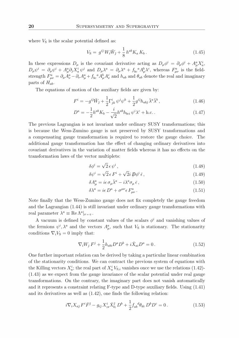
20 Supersymmetry and Supergravity
where VS is the scalar potential defined as:
VS = giWiW +1
8habKaKb . (1.45)
In these expressions Dµ is the covariant derivative acting as Dµφi = ∂µφ
i + AaµXia,
Dµψi = ∂µψ
i + Aaµ∂jXia ψ
j and Dµλa = ∂µλ
a + f abc A
bµλ
c, whereas F aµν is the field-
strength F aµν = ∂µA
aν−∂νAaµ+f a
bc AbµA
cν and hab and θab denote the real and imaginary
parts of Hab.
The equations of motion of the auxiliary fields are given by:
F i = −giW +1
2Γijk ψ
jψk +1
2gihab λ
aλb , (1.46)
Da = −1
2habKb −
i√2habhbci ψ
iλc + h.c. . (1.47)
The previous Lagrangian is not invariant under ordinary SUSY transformations; this
is because the Wess-Zumino gauge is not preserved by SUSY transformations and
a compensating gauge transformation is required to restore the gauge choice. The
additional gauge transformation has the effect of changing ordinary derivatives into
covariant derivatives in the variation of matter fields whereas it has no effects on the
transformation laws of the vector multiplets:
δφi =√
2 ε ψi , (1.48)
δψi =√
2 ε F i +√
2iD/ φi ε , (1.49)
δAaµ = iε σµλa − iλaσµ ε , (1.50)
δλa = iεDa + σµνε F aµν . (1.51)
Note finally that the Wess-Zumino gauge does not fix completely the gauge freedom
and the Lagrangian (1.44) is still invariant under ordinary gauge transformations with
real parameter λa ≡ Re Λa|θ = 0 .
A vacuum is defined by constant values of the scalars φi and vanishing values of
the fermions ψi, λa and the vectors Aaµ, such that VS is stationary. The stationarity
conditions ∇iVS = 0 imply that:
∇iWj Fj +
1
2habiD
aDb + iXaiDa = 0 . (1.52)
One further important relation can be derived by taking a particular linear combination
of the stationarity conditions. We can contract the previous system of equations with
the Killing vectors X ia; the real part of X i
a VS,i vanishes once we use the relations (1.42)-
(1.43) as we expect from the gauge invariance of the scalar potential under real gauge
transformations. On the contrary, the imaginary part does not vanish automatically
and it represents a constraint relating F-type and D-type auxiliary fields. Using (1.41)
and its derivatives as well as (1.42), one finds the following relation:
i∇iXa FiF − giX i
(aXb) D
b +1
2f dab θdcD
bDc = 0 . (1.53)
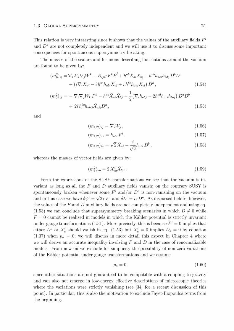
1.3. Global Supersymmetry 21
This relation is very interesting since it shows that the values of the auxiliary fields F i
and Da are not completely independent and we will use it to discuss some important
consequences for spontaneous supersymmetry breaking.
The masses of the scalars and fermions describing fluctuations around the vacuum
are found to be given by:
(m20)i =∇iWk∇W
k −Rikl FkF l + habXaiXb + habhacihbdD
bDc
+(i∇iXa − i hbchabiXc + i hbchabjXci
)Da , (1.54)
(m20)ij = −∇i∇jWk F
k − habXaiXbj −1
2
(∇ihabj − 2hcdhacihbdj
)DaDb
+ 2i hbchab(iXcj)Da , (1.55)
and
(m1/2)ij = ∇iWj , (1.56)
(m1/2)ab = habi Fi , (1.57)
(m1/2)ia =√
2 Xai −i√2habiD
b , (1.58)
whereas the masses of vector fields are given by:
(m21)ab = 2X i
(aXb)i . (1.59)
Form the expressions of the SUSY transformations we see that the vacuum is in-
variant as long as all the F and D auxiliary fields vanish; on the contrary SUSY is
spontaneously broken whenever some F i and/or Da is non-vanishing on the vacuum
and in this case we have δψi =√
2 ε F i and δλa = i εDa. As discussed before, however,
the values of the F and D auxiliary fields are not completely independent and using eq.
(1.53) we can conclude that supersymmetry breaking scenarios in which D 6= 0 while
F = 0 cannot be realized in models in which the Kahler potential is strictly invariant
under gauge transformations (1.31). More precisely, this is because F i = 0 implies that
either Da or X ia should vanish in eq. (1.53) but X i
a = 0 implies Da = 0 by equation
(1.37) when pa = 0; we will discuss in more detail this aspect in Chapter 4 where
we will derive an accurate inequality involving F and D in the case of renormalizable
models. From now on we exclude for simplicity the possibility of non-zero variations
of the Kahler potential under gauge transformations and we assume
pa = 0 (1.60)
since other situations are not guaranteed to be compatible with a coupling to gravity
and can also not emerge in low-energy effective descriptions of microscopic theories
where the variations were strictly vanishing (see [34] for a recent discussion of this
point). In particular, this is also the motivation to exclude Fayet-Iliopoulos terms from
the beginning.
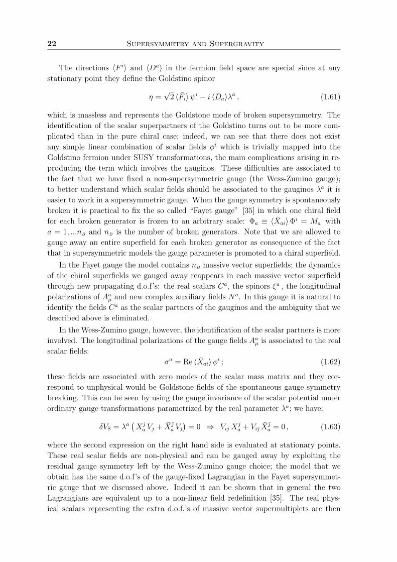
22 Supersymmetry and Supergravity
The directions 〈F i〉 and 〈Da〉 in the fermion field space are special since at any
stationary point they define the Goldstino spinor
η =√
2 〈Fi〉ψi − i 〈Da〉λa , (1.61)
which is massless and represents the Goldstone mode of broken supersymmetry. The
identification of the scalar superpartners of the Goldstino turns out to be more com-
plicated than in the pure chiral case; indeed, we can see that there does not exist
any simple linear combination of scalar fields φi which is trivially mapped into the
Goldstino fermion under SUSY transformations, the main complications arising in re-
producing the term which involves the gauginos. These difficulties are associated to
the fact that we have fixed a non-supersymmetric gauge (the Wess-Zumino gauge);
to better understand which scalar fields should be associated to the gauginos λa it is
easier to work in a supersymmetric gauge. When the gauge symmetry is spontaneously
broken it is practical to fix the so called “Fayet gauge” [35] in which one chiral field
for each broken generator is frozen to an arbitrary scale: Φa ≡ 〈Xai〉Φi = Ma with
a = 1, ...nB and nB is the number of broken generators. Note that we are allowed to
gauge away an entire superfield for each broken generator as consequence of the fact
that in supersymmetric models the gauge parameter is promoted to a chiral superfield.
In the Fayet gauge the model contains nB massive vector superfields; the dynamics
of the chiral superfields we gauged away reappears in each massive vector superfield
through new propagating d.o.f’s: the real scalars Ca, the spinors ξa , the longitudinal
polarizations of Aaµ and new complex auxiliary fields Na. In this gauge it is natural to
identify the fields Ca as the scalar partners of the gauginos and the ambiguity that we
described above is eliminated.
In the Wess-Zumino gauge, however, the identification of the scalar partners is more
involved. The longitudinal polarizations of the gauge fields Aaµ is associated to the real
scalar fields:
σa = Re 〈Xai〉φi ; (1.62)
these fields are associated with zero modes of the scalar mass matrix and they cor-
respond to unphysical would-be Goldstone fields of the spontaneous gauge symmetry
breaking. This can be seen by using the gauge invariance of the scalar potential under
ordinary gauge transformations parametrized by the real parameter λa; we have:
δVS = λa(Xja Vj + X
a V)
= 0 ⇒ Vij Xja + Vi X
a = 0 , (1.63)
where the second expression on the right hand side is evaluated at stationary points.
These real scalar fields are non-physical and can be gauged away by exploiting the
residual gauge symmetry left by the Wess-Zumino gauge choice; the model that we
obtain has the same d.o.f’s of the gauge-fixed Lagrangian in the Fayet supersymmet-
ric gauge that we discussed above. Indeed it can be shown that in general the two
Lagrangians are equivalent up to a non-linear field redefinition [35]. The real phys-
ical scalars representing the extra d.o.f.’s of massive vector supermultiplets are then
1.3. Global Supersymmetry 23
naturally identified with the fields:
ρa = Im 〈Xai〉φi ; (1.64)
it is easy to verify that these fields, in the supersymmetric limit in which all the F
and D auxiliary fields vanish, have the same masses of the gauge vector fields. It
is also interesting to note that, when the gauge symmetry is not broken and all the
〈X ia〉 vanish, we have that σa = ρa = 0 as is to be expected since in this case Aaµ’s
have only two d.o.f and there are no physical propagating scalars associated to vector
multiplets. Notice that a priori the gauge part in the Goldstino field (1.61) may be
different from zero even when the gauge symmetry is not broken; in this case there still
remains a problem related to the identification of the scalar partner of the Goldstino
since the previous analysis does not apply. However we have seen that this situation
can be realized only if there are non-trivial holomorphic functions pa in the gauge
transformations of the Kahler potential and we have excluded this possibility.
The previous analysis shows that in the Wess-Zumino gauge the supersymmetric
structure of massive vector multiplets is not manifest in the Lagrangian and this com-
plicates the identification of the scalar partner of the Goldstino; in particular it is not
easy to find a linear combination of scalars which transforms into η under supersym-
metry transformations. We can however define a projected Goldstino η′ =√
2 〈Fi〉ψito which we can associate, without ambiguity, the projected sGoldstino:
φ =√
2 〈Fi〉φi . (1.65)
Under SUSY transformations one then finds δϕ =√
2 ε η′ and also in this case the
complex sGoldstino field describes two real scalar fields whose masses are entirely
controlled by supersymmetry breaking effects. We will see in Chapter 4 that these
special modes play a relevant role for discussing the stability properties of the scalar
potential. The previous analysis, however, suggests that also the special direction
Im 〈DaXai〉 (1.66)
should be somehow associated to the scalar superpartners of the Goldstino. This
suggests that the value of the scalar mass matrix projected on this direction should
not be completely arbitrary. This argument will be discussed in more detail in Chapter
4 where the role of the directions 〈F i〉 and 〈X ia〉 for the study of vacuum stability is
extensively analyzed.
We conclude this section by recalling the expression of the supertrace for non-linear
gauged σ-models [29]:
sTr[m2] ≡ Tr[m20]− 2 Tr[m2
1/2] + 3 Tr[m21]
= 2(Ri − hachbdhabihcd
)F iF
+ i(∇iXa + 2hbchabiX
ic
)Da + h.c. .
(1.67)
The implications of this formula for SUSY phenomenology are discussed in the next
chapter.
24 Supersymmetry and Supergravity
1.4 Local Supersymmetry
In this section we will review in some detail the basic ideas and procedures to construct
locally supersymmetric invariant models. For simplicity we start as before by consid-
ering models containing only chiral multiplets and then we discuss the generalization
including gauge symmetries and vector multiplets.
1.4.1 Models with only Chiral Multiplets
There exist several different versions of N = 1 supergravity; each formulation is charac-
terized by a different choice of the auxiliary fields that are included in the gravitational
sector together with the graviton and the gravitino. Here will focus on the so called
“old minimal supergravity” [36, 37] in which the off-shell supergravity multiplet, in
addition to the graviton eaµ and the gravitino ψαµ fields, contains two auxiliary fields
namely one complex scalar Fφ and one vector field Aµ :eaµ, ψ
αµ , Aµ, Fφ
. (1.68)
Supergravity can be obtained as a gauge theory of the Super-Poincare group, pro-
vided that certain constraints are implemented to remove non-physical gauge d.o.f’s
in the gravitational sector. Since the concept of supergravity as a gauge theory plays
a fundamental role in our derivation of the Lagrangian, we shall clarify this point
by briefly recalling how General Relativity can be obtained as a gauge theory of the
Poincare group. This idea is implemented by the so called Cartan formalism 5 which
consists in introducing a vierbein eaµ, which is the gauge field associated to local transla-
tions Pa and a spin connection ωabµ , which is the gauge field associated to local Lorentz
transformations Mab. General Relativity can be obtained by gauging the Poincare
group and by imposing the torsion-free constraint, which fixes the spin connection as a
function of the vierbein. The reason why this constraint must necessarily be imposed
to recover ordinary General Relativity can be understood in the following way: the
generator Pa is associated to local translations and satisfies the algebra [δ1P , δ
2P ] = 0;
however General Relativity requires invariance under general coordinate transforma-
tions (diffeomorphisms) which in general do not commute. The standard procedure
to convert local translations to general coordinate transformations is to impose that
the torsion tensor vanishes. In this case the group algebra must be modified since the
constraint turns out to be non-invariant under local translations. In other words, we
need to define new transformation laws δP ≡ δP + δ′ to compensate the non vanish-
ing transformation of the constraint and, in general, the new transformations will not
commute as expected for diffeomorphisms. We will see that this construction can be
generalized also to derive the supergravity Lagrangian.
As for the case of ordinary gauge theories, one can choose among three different
approaches to construct locally supersymmetric theories; let us recall them:
5See [38] for a comprehensive introduction to Cartan’s formalism.
1.4. Local Supersymmetry 25
1. The Noether approach, which is the standard procedure by which the invari-
ance under local transformations is implemented, at the level of the component
Lagrangian, by coupling the gauge vectors to the conserved currents of global
symmetries; when necessary, gauge invariance must be enforced by adding extra
terms to compensate for the non-vanishing variation of the action [39–41] (see
also [42]).
2. The superspace approach, which generalizes the geometric techniques of gauge
theories to superspace. For ordinary gauge theories, it reduces to introduce a
gauge connection Aaµ,α,α for each generator of the symmetry group in order
to define supersymmetric gauge covariant derivatives and field strengths. For
gravitational interactions, however, this approach implies further complications
since it requires the study of curved superspaces geometry; this implies also that
one has to generalize ordinary superfields to be functions of curved superspace
coordinates [25, 43].
3. The tensor calculus approach, in which the ordinary (rigid) SUSY tensor calculus
gets properly “covariantized”. In this case, one works with standard (global)
superfields in which space-time derivatives are replaced by covariant derivatives
and the component fields transform covariantly under both gauge and SUSY
transformations [44, 45].
The first approach, even if didactically more enlightening, turns out to be quite cum-
bersome; this is because in general the procedure must be implemented several times
and at each step new terms must be introduced to compensate for the variation of
the action. In the second approach, the gauge group is maximally extended in order
to implement gauge transformations on the whole superspace; this introduces several
new gauge fields which must finally be fixed by performing appropriate gauge choices
and by imposing several covariant constraints. This procedure, though more appealing
from a geometrical point of view, is rather tedious and not particularly enlightening.
In this work we will use the third formalism to construct the supergravity La-
grangian. This approach may appear less elegant than the one in superfields but it has
the advantage that it requires to manipulate only the minimal set of physical (grav-
itational) gauge fields. Moreover, the tensor calculus is only slightly modified with
respect to the rigid one and it is possible to exploit all the powerful machinery of or-
dinary superfields. Finally we anticipate that, in general, also in this formalism it is
necessary to impose some constraints to discard unphysical gauge d.o.f.’s but, in our
opinion, the few constraints that one has to impose are less arbitrary and more easy to
be solved than those of the curved superspace approach. These constraints are essen-
tially of the same nature as the torsion-free constraint in ordinary General Relativity
described above. Summarizing, in the following we adopt the tensor calculus approach
to construct SUGRA as a gauge theory since, from a technical point of view, it is the
most efficient for our purposes.
26 Supersymmetry and Supergravity
Historically, there exist two different formalisms based on the tensor calculus ap-
proach. The references we gave at the point 3 above refer to the construction of
supergravity as a gauge theory of the super-Poincare group; on the other hand, one
can also obtain minimal supergravity as a gauge theory of the superconformal group
[46–49]. This alternative is not peculiar of supersymmetry; also ordinary General Rel-
ativity can be obtained as a gauged-fixed version of a scale invariant theory. Indeed,
we can promote General Relativity to be scale invariant by adding a new real scalar
field φ called compensator which transforms in a suitable way under local scale (Weyl)
transformations:
L =1
2
∫d4x√−g [
1
6φ2R + ∂µφ∂
µφ ] , (1.69)
where the transformation laws of the metric and compensator are:
δgµν(x) = −2λ(x) gµν(x) , δφ(x) = λ(x)φ(x) . (1.70)
General Relativity in the Einstein frame is then obtained after gauge-fixing the extra
symmetry by imposing φ =√
3/4πGN . One may wonder why it is convenient to opt
for the superconformal approach, which a priori looks more complicated; indeed, the
conformal group has 15 generators instead of 10 and it will be necessary to impose
more constraints to fix the extra gauge symmetries. The answer to this question is
related to the intimate nature of the scalar auxiliary field Fφ in the minimal SUGRA
multiplet. The main feature of the superconformal approach is that, in this formalism,
Fφ is disentangled from the rest of the gravitational multiplet. It belongs to a different
supermultiplet, called conformal compensator multiplet, which has the same function
of the compensator φ that we discussed above. Fφ is the only field in the gravitational
sector that can affect the scalar potential; for this reason, having a formalism in which
Fφ can be manipulated avoiding all the complications introduced by the other gravita-
tional fields, is very attractive. As we are going to see, the computation of the scalar
potential and the scalar masses in this formalism can be done in a very economical
way.
Superconformal Supergravity
Let us start by reviewing the main ingredients that are necessary to construct the su-
pergravity Lagrangian in the superconformal formalism. In this analysis we will follow
the notation and the arguments of [48] (see also [50] for a review). The group of super-
conformal transformations is generated by the 15 bosonic generators of the conformal
group: Pa for local translations, Mab for local Lorentz transformations, Ka for local
special conformal transformations and D for local dilatations. In addition there are 2
kinds of fermionic supersymmetry generators Qα and Sα and one generator TR associ-
ated to a local U(1)R R-symmetry. The gauge fields associated to each transformation
are summarized in Tab. 1.1, where we use greek letters for global indices and latin
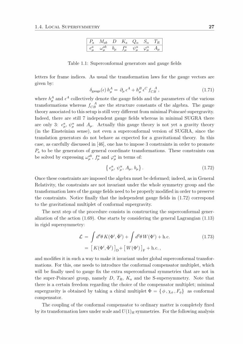
1.4. Local Supersymmetry 27
Pa Mab D Ka Qα Sα TReaµ ωabµ bµ faµ ψαµ ϕαµ Aµ
Table 1.1: Superconformal generators and gauge fields
letters for frame indices. As usual the transformation laws for the gauge vectors are
given by:
δgauge(ε)hAµ = ∂µ ε
A + hBµ εC f A
CB , (1.71)
where hAµ and εA collectively denote the gauge fields and the parameters of the various
transformations whereas f ACB are the structure constants of the algebra. The gauge
theory associated to this setup is still very different from minimal Poincare supergravity.
Indeed, there are still 7 independent gauge fields whereas in minimal SUGRA there
are only 3: eaµ, ψαµ and Aµ. Actually this gauge theory is not yet a gravity theory
(in the Einsteinian sense), not even a superconformal version of SUGRA, since the
translation generators do not behave as expected for a gravitational theory. In this
case, as carefully discussed in [46], one has to impose 3 constraints in order to promote
Pa to be the generators of general coordinate transformations. These constraints can
be solved by expressing ωabµ , faµ and ϕαµ in terms of:eaµ, ψ
αµ , Aµ, bµ
. (1.72)
Once these constraints are imposed the algebra must be deformed; indeed, as in General
Relativity, the constraints are not invariant under the whole symmetry group and the
transformation laws of the gauge fields need to be properly modified in order to preserve
the constraints. Notice finally that the independent gauge fields in (1.72) correspond
to the gravitational multiplet of conformal supergravity.
The next step of the procedure consists in constructing the superconformal gener-
alization of the action (1.69). One starts by considering the general Lagrangian (1.13)
in rigid supersymmetry:
L =
∫d4θ K(Φi, Φı) +
∫d2θW (Φi) + h.c. (1.73)
=[K(Φi, Φı)
]D
+[W (Φi)
]F
+ h.c. ,
and modifies it in such a way to make it invariant under global superconformal transfor-
mations. For this, one needs to introduce the conformal compensator multiplet, which
will be finally used to gauge fix the extra superconformal symmetries that are not in
the super-Poincare group, namely D, TR, Ka and the S-supersymmetry. Note that
there is a certain freedom regarding the choice of the compensator multiplet; minimal
supergravity is obtained by taking a chiral multiplet Φ = φ , χφ , Fφ as conformal
compensator.
The coupling of the conformal compensator to ordinary matter is completely fixed
by its transformation laws under scale and U(1)R symmetries. For the following analysis
28 Supersymmetry and Supergravity
we refer to [51]. The Lagrangian (1.73) must have conformal weight (dimension)
d(L) = 4 and chiral weight (R-charge) R(L) = 0. Since d(θα) = −12
and R(θα) = 1,
this implies that:
d(K) = 2 , d(W ) = 3 ; (1.74)
R(K) = 0 , R(W ) = 2. (1.75)
To find the right powers of the compensator field which should be inserted in each term
of the supersymmetric Lagrangian it is useful to assume, without loss of generality, that
matter fields have vanishing conformal weight d(φi) = 0 and vanishing chiral weight
R(z) = 0, whereas the compensator has d(φ) = 1; this fixes also R(φ) = 2/3 since it
is possible to show that the conformal and the chiral weights are not independent for
chiral multiplets. Note that having matter chiral superfields with zero mass dimension
is not a problem since, in the end, it is possible to perform a field redefinition to restore
the right dimensions.
From the previous analysis, one can guess the proper coupling of the conformal
compensator to matter fields in superconformal supergravity:
L =[K(Φi, Φı) ΦΦ
]D
+[W (Φi) Φ3
]F
+ h.c. . (1.76)
Note that we did not express the Lagrangian in terms of integrals over (rigid) spinor
coordinates θα. This is because ordinary D and F terms cannot be used to construct
covariant actions of the type∫d4x e [ ]D +
∫d4x e [ ]F , where e is the determinant of
the vierbein. The problem is that ordinary F and D terms do not transform properly
under local supercovariant transformations, and some new terms must be added to
obtain invariant actions. As explained in [48] (see also [52] for conventions compatible
with ours), the right expression for the superconformal F -term that should be used to
construct locally superconformal invariant action is :∫d4x [ Σ ]F , [ Σ ]F = e
(F − i
√2χσµψµ − z ψµσµνψν
), (1.77)
where Σ = z, χ, F is a chiral multiplet with conformal weight d(Σ) = 3 as required in
the Lagrangian (1.76). The expression for the the superconformally invariant D-term
is slightly more complicated; we just recall the most interesting terms:∫d4x [ Ω ]D , [ Ω ]D = e
( 1
2D − 1
2(λσµψµ − i ξσµνDcµψν + h.c )
+C
3
( 1
2R− 1
eL0
RS
))+ ... , (1.78)
where Ω = C, ξ,M,Bµ, λ,D is a vector multiplet with conformal weight d(Ω) =
2; L0RS represents the standard kinetic term of the Rarita-Schwinger action for the
gravitino ψαµ , whereas the ellipsis represents terms quadratic and cubic in the gravitino
multiplied by the vector and spinorial components of Ω which do not contribute to the
gravitino mass. Note finally that the function K in the superconformal Lagrangian
1.4. Local Supersymmetry 29
(1.76) is not what is called Kahler potential in the supergravity literature; in order
to recover the canonical form of the kinetic terms of the matter multiplets one has to
perform the redefinition K → −3M2P e−K/3M2
P .6 Setting M2P = 1 one finally obtains
the Lagrangian of superconformal supergravity:
L =[−3 e−K/3 ΦΦ
]D
+[W Φ3
]F
+ h.c. . (1.79)
Notice that, in order to obtain the full Poincare supergravity Lagrangian in com-
ponent fields, one has now to gauge-fix the extra-symmetries in (1.79) by using the
compensator superfield. As a matter of fact, however, it is often convenient to work
with the full superconformally invariant Lagrangian, manipulating the compensator
superfield as an ordinary matter chiral superfield, and substitute its gauge-fixed ex-
pression only at the very end of the computations. This is because, as argued in
[48] (see also [53]) the superconformal tensor calculus is substantially simpler than the
super-Poincare tensor calculus. It turns out that under ordinary SUSY transformations
generated by Qα, superconformal multiplets transform in the usual way (1.16)-(1.18)
with the only change that ordinary space-time derivatives must be replaced by super-
conformal covariant derivatives. Also the multiplet components and the tensor calculus
are easily covariantized by using the same technique. This makes it is possible to use
rigid SUSY superfields to represent a superconformal chiral multiplets Φi = φi, χi, F iin the following way:
Φi(x, θ, θ) = φi +√
2 θχi + θ2F i (1.80)
+ i θσµθDcµφi −i√2θ2Dcµχiσµθ +
1
4θ2DcµDcµ φi ;
where Dcµ = ∂µ−haµTa is the conformal covariant derivative and the sum over the group
generators Ta excludes the local translations Pa. A similar (rigid-like) covariantized ex-
pression can be defined also for vector multiplets. The results of superconformal tensor
calculus can be smartly reproduced by multiplying the above-defined “covariantized”
superfields; for example the highest components of the real multiplet obtained by taking
the product of one chiral and one anti-chiral multiplet is given by:
ΦiΦı = ... + θ2θ2 [F iF ı −DcµφıDcµφi − i χıσµDcµχi ] + tot. deriv. . (1.81)
Using these results, it is easy to understand which is the fundamental simplification
introduced by this formalism. Indeed, if one focuses only on the scalar potential, it is
possible to discard the gravitational gauge fields eaµ, ψαµ and Aµ, and the expressions
for the supercovariant F -terms (1.77) and D-terms (1.78) then reduce to the usual
ones in rigid supersymmetry. Moreover, in this case also the expressions (1.80) and
(1.81) reduce to the ordinary ones, so that the tensor calculus works exactly as in rigid
superspace. One can then rewrite (1.79) in terms of rigid superspace integrals:
L =
∫d4θ
(−3 e−K/3 ΦΦ
)+
∫d2 θW Φ3 + h.c. + ... , (1.82)
6A more detailed discussion of this part can be found for example in [50].
30 Supersymmetry and Supergravity
where the ellipsis indicates the gravitational terms which do not admit a simple expres-
sion in terms of integral over the rigid superspace and are usually expressed directly in
components fields.7
The last aspect we need to discuss is the gauge-fixing of the extra symmetries of
the superonformal group [54] (see also [52]). The special conformal transformations Ka
can be fixed by setting the dilatation gauge field to zero:
bµ = 0 . (1.83)
In order fix D, TR and Sα symmetries, it is useful to redefine the compensator multiplet
in the following way:
Φ = φ 1 , χφ , U , φ = |φ|eiσ , (1.84)
where we defined the normalized auxiliary field U as:
Fφ = φU . (1.85)
One common gauge choice consists in using the modulus and the phase of the scalar
φ to fix D and TR, and the spinor χφ to fix the S-supersymmetry; the field U is left
unfixed and, together with Aµ, it is an auxiliary field of the Poincare gravitational
multiplet (1.68). The actual values at which the fields are fixed are chosen in order
simplify as much as possible the resulting Lagrangian. |φ| is fixed in such a way that
the kinetic term of graviton is canonically normalized (Einstein frame); by inspection
of (1.78), one is led to chose:
C ≡ −3 |φ|2 e−K/3 = −3 ⇒ |φ| = eK/6 . (1.86)
The phase of φ can be fixed in such a way that the gravitino mass is real; the relevant
term to consider is −z ψµσµνψν . This suggests the following choice:
Im z ≡ Im(φ3W ) = 0 ⇒ σ =i
6(logW − log W ) . (1.87)
Finally χφ is fixed in such a way to cancel the non-canonical mixing i ξσµν∂µψν in the
gravitino kinetic term. This implies:
ξ ≡ 3i√
2 |φ|2 e−K/3(χφ −
1
3Kiχ
i
)= 0 ⇒ χφ =
1
3Ki χ
i . (1.88)
After the gauge fixing we then get:
Φ = exp
[1
6(K − logW + log W )
]·
1 ,1
3Ki χ
i , U
. (1.89)
7Examples of applications in which one is not allowed to naively ignore these terms are discussedin [52]; in such situations, the authors propose to use a smarter gauge choice which produces someuseful simplifications.
1.4. Local Supersymmetry 31
This gauge, proposed in [54], is very useful since it avoids the field redefinitions which
are usually needed to recover the canonical kinetic terms and masses for the graviton
and the gravitino.
The compensator field and the SUGRA Lagrangian (1.79) are usually rewritten in a
more compact form by exploiting the invariance of the action under generalized Kahler
transformations. Under these transformations the Kahler potential, the superpotential
and the compensator field transform in the following way:
( Φ , K , W )→ ( Φ eY/3 , K + Y + Y , W e−Y ) . (1.90)
By choosing Y = logW we obtain:
L =[−3 e−G/3 ΦΦ
]D
+[
Φ3]F
+ h.c (1.91)
where:
G(Z, Z) = K(Z, Z) + logW (Z) + log W (Z) (1.92)
and the new compensator multiplet is given by:
Φ = eG/6 ·
1 ,1
3Gi χ
i , U
. (1.93)
We conclude this discussion on the superconformal gauge fixing by recalling that the
ordinary supersymmetry transformations of Poincare SUGRA emerge as a combination
of supersymmetry and extra conformal transformations which preserves the supercon-
formal gauge choice; this is similar to what happens in ordinary supersymmetric gauge
theories, in which supersymmetry transformations must be modified in order to pre-
serve the Wess-Zumino gauge choice, see eq. (1.48)-(1.51).
Let us now recall the expressions for the scalar potential and the mass matrix of
scalar fields in the non-linear σ-model coupled to gravity [55, 56]. As already discussed,
these quantities can be efficiently computed by using the superfield version of the
SUGRA Lagrangian (1.91):
L =
∫d4θ[−3 e−G(Φi,Φı)/3 ΦΦ
]+
∫d2θΦ3 + h.c + ... . (1.94)
After eliminating the auxiliary fields of the matter and the compensator chiral multi-
plets, one finally finds:
VS = eG (GkGk − 3 ) . (1.95)
A vacuum is defined by constant values of the scalar fields for which VS is stationary
whereas spinor and tensor fields must have vanishing expectation values in order to
preserve Lorentz invariance. The stationarity conditions have the form:
Gi +Gk∇iGk = 0 , (1.96)
32 Supersymmetry and Supergravity
and at any stationary point the auxiliary fields of the compensator and of chiral matter
multiplets are given respectively by the expressions:
U = eG/2 ( 1− 1
3GkGk ) , (1.97)
F i = −eG/2 giG . (1.98)
The expectation value 〈VS〉 defines the cosmological constant, which must be almost
vanishing (' 10−3eV), as suggested by cosmological observations [57]; this implies that
the space-time must be approximately Minkowski. Note that a small value of the
cosmological constant is not stable against quantum corrections and can be achieved
only by a severe fine tuning of the parameters in the Lagrangian. This is the so called
cosmological constant problem [58]; it has the same nature of the hierarchy problem
that we discussed in the first section of this chapter but in this case the amount of
fine-tuning is dramatically larger: 120 order of magnitudes! We see that the condition
for a vanishing cosmological constant is given by:
VS = 0 ⇒ GiGi = 3 . (1.99)
The masses of scalar fields are found to be:
(m20)i = eG∇iGk∇G
k −Rikl Fk F l +m2
3/2 gi , (1.100)
(m20)ij = −eG/2 F k∇(i∇j) Gk + 2m2
3/2∇(iGj) , (1.101)
where we have introduced the gravitino mass given by:
m3/2 = eG/2 . (1.102)
The mass mixing term involving the gravitino and matter fermions has instead the
form:
− i2
√2 〈eG/2Gi〉χi σµ ψµ + h.c. . (1.103)
From this expression we recognize that the Goldstino is defined by the direction 〈Gi〉in the spinor field space. This can also be seen by using the SUSY transformation
laws of matter fields; indeed it is possible to show that the only non-homogeneous
transformation on the vacuum is [25]:
δχi = −√
2 ε 〈eG/2Gi〉 =√
2ε 〈F i〉 . (1.104)
This expression shows that SUSY is broken in SUGRA whenever 〈Gi〉 6= 0. In super-
gravity, however, the Goldstino is not a physical degree of freedom and it can be gauged
away by a proper gauge choice; in common language one says that it is “eaten” by
the massive gravitino through the super-Higgs mechanism [59]. When the cosmological
constant vanishes we can define the normalized Goldstino as:
η =
√2√3m3/2 〈Gi〉χi. (1.105)
1.4. Local Supersymmetry 33
The associated scalar superpartner, the sGoldstino, is defined as:
ϕ =
√2√3m3/2 〈Gi〉φi. (1.106)
This transforms under SUSY as δϕ =√
2 ε η.
1.4.2 Models with Chiral and Vector Multiplets
Let us now recall the main ingredients of the non-linear gauged σ-model coupled to
gravity [60, 49]; for an exhaustive review of this part see also [61]. The generalization of
the previous construction to include ordinary gauge symmetries and vector multiplets
does not present any important complication. The suitable coupling of the compensator
multiplet to the gauge fields can be guessed by performing the same analysis as for
chiral multiplets, which was based on the transformation properties of the compensator
under superconformal transformations. It turns out that there is no dependence on Φ
in the gauge kinetic Lagrangian; this is because assuming d(V ) = 0 and R(V ) = 0 it
is easy to see that:
d(WαaW aα) = 3 , R(WαaW a
α) = 2 . (1.107)
Superconformal invariance then implies that a coupling between the compensator
and the vector multiplets can only arise in the non-holomorphic part of the Lagrangian.
It is easy to promote the Lagrangian (1.35) to be superconformal invariant:
L =[−3 e−K/3 ΦΦ
]D
+[W Φ3
]F
+1
4
[Hab(Φ
i)WαaW bα
]F
+ h.c , (1.108)
where [ ]D and [ ]F have the same expressions we gave in the previous section. In
particular, it is still true that the computation of the scalar potential and the mass
matrix of the scalar fields can be more efficiently performed by rewriting the previous
lagrangian as an integral over rigid superspace:
L =
∫d4θ[−3 exp
− 1
3G(Φi, Φı, V )
]ΦΦ +
(∫d2θΦ3 + h.c.
)+
(∫d2θ
1
4Hab(Φ
i)W aαW bα + h.c.
)+ ... , (1.109)
where, again, the terms that we discard depend on the non-scalar fields of the gravi-
tational supermultiplet. In addition, the same gauge fixing of the extra symmetries of
the superconformal group can be applied [54] and the compensator multiplet has the
same form:
Φ = eG/6 ·
1 ,1
3Gi χ
i , U
. (1.110)
where G(Φi, Φı) and its derivative are evaluated at V a = 0.
34 Supersymmetry and Supergravity
As for pure chiral models, the gauge vectors are associated to the gauging of the
isometry group of the target space of scalar fields; in this case one must require that
G(Φi, Φı, V ) is strictly invariant under gauge transformations generated by the holo-
morphic Killing vectors X ia associated to the isometries of the metric Gi . In order to
easily manipulate the Lagrangian (1.109), it is useful to fix the Wess-Zumino gauge
for the internal gauge symmetries; we can then develop the integrand of the non-
holomorphic part of the lagrangian Ω = −3e−13GΦΦ as:
Ω = −3 e−13G ΦΦ +Ga e
− 13G ΦΦV a +
1
2
(Gab −
1
3GaGb
)e−
13G ΦΦV a V b (1.111)
where G and its derivatives with respect to vector fields are now evaluated at V a = 0.
As before, the relevant functions Ga(Φi, Φı) and Gab(Φ
i, Φı) are determined by using
the invariance condition δ G(Φi, Φı, V ) = 0 and taking multiple derivatives. We finally
obtain:
X iaGi −
i
2Ga = 0 , (1.112)
X ia =
i
2giGa , (1.113)
Gab = 4 giXi(a X
b) . (1.114)
The second expression shows that the Killing potentials for X ia can be identified with
−12Ga The transformation properties of the gauge kinetic function are fixed by re-
quiring the gauge invariance of the kinetic Lagrangian of the vector multiplets. This
implies:
X iaHbci = −2f d
a(bHc)d . (1.115)
The last useful relation comes from the equivariance condition of the Killing vectors,
which guarantees that the Killing potentials can be chosen in the adjoint representation:
giXi[aX
b] =
i
4f cab Gc . (1.116)
Again we avoid to present the full expression of the Lagrangian and we focus on the
scalar potential and the masses, which can be easily computed from the Lagrangian
(1.109) by exploiting the superfield machinery. In particular, as in the previous case, we
can manipulate the compensator as an independent chiral superfield and substitute its
gauge-fixed expression (1.110) only at the very end of the computation. Moreover, since
we are interested mainly in the scalar part of the Lagrangian, the spinor components
of matter, gauge and compensator superfield can be set to zero..
The scalar potential is found to be:
VS = eG(GkGk − 3
)+
1
8habGaGb , (1.117)
1.4. Local Supersymmetry 35
where hab represents the real part of the gauge kinetic function Hab and we used the
scalar parts of the equations of motion of the auxiliary fields F i and Da, which give:
F i = −eG/2 giG , (1.118)
Da = −1
2habGb . (1.119)
The vacuum is defined by constant values of the scalar fields for which VS is stationary.
As already discussed, for phenomenological reasons we shall require a vanishing vacuum
energy (flatness condition); this gives the relation:
−3 +GiGi +1
8e−GGaGa = 0 . (1.120)
The stationarity conditions are then given by:
Gi +Gk∇iGk +1
4e−G
[Ga(∇i −
1
2Gi
)Ga −
1
2habiG
aGb]
= 0 . (1.121)
In this case too, one can deduce from the stationarity conditions a relation between
F and D auxiliary fields which is valid at any stationary point. Following [61] we
multiply the stationarity condition by X ia and consider the two independent relations
given by the real and imaginary parts. The real part is trivial and vanishes because of
gauge invariance of the scalar potential under ordinary (real) gauge transformations.
The imaginary part insted does not vanish automatically and gives a “dynamical”
constraint between F and D terms which is valid at any stationary point. Using the
relations (1.112) and (1.113),8 one finds [61–64]:
i∇iXaFiF − giX i
aXb D
b +1
2f dab θdcD
bDc − (FiFi −m23/2)Da . (1.123)
where m3/2 is the gravitino mass which is defined as in the previous section as:
m3/2 = eG/2 . (1.124)
In SUGRA, however, there exists another “kinematical” constraint between F and D
auxiliary fields which is valid, contrarily to the previous one, at any point of the scalar
field space. It follows directly from (1.112), which gives:
Da = ihab
m3/2
XbiFi = −i h
ab
m3/2
XbıFı. (1.125)
This constraint is purely gravitational and it becomes trivial in the rigid limit MP →∞and m3/2 → 0 whereas the “dynamical” constraint reduces to expression (1.53) in the
8One also needs to use the relation
Xia +Xj∇iGk +Gj∇iXj
a = 0 , (1.122)
which can be obtained by taking one covariant derivative of the equation that expresses the invarianceof G(Φi, Φı) under isometry transformations.
36 Supersymmetry and Supergravity
same limit. The rigid limit is performed by sending also m3/2 to zero. This corresponds,
in a flat space, to keep the SUSY breaking scale fixed. In this case too, it is possible
to use the above constraints to derive interesting bounds on the ratio between F and
D auxiliary fields, which have important consequences for SUSY breaking scenarios.
Using the stationarity and the flatness conditions, it is possible to show that the
mass matrices of scalar fields are given by [61]:
(m20)i = eG∇iGk∇G
k −RiklFkF l + habXaiXb +m2
3/2 gi
− 1
2
(gi −GiG
)DaDa +
(G(ihab) + hcdhacihbd
)DaDb
+(i∇iXa − i hbchabiXc + i hbchabjXci
)Da
−(i GiXa − i GXai
)Da , (1.126)
(m20)ij = −eG/2 F k∇(i∇j)Gk − habXaiXbj + 2m2
3/2∇(iGj)
− 1
2
(∇ihabj − 2hcdhacihbdj − 2G(ihabj)
)DaDb
− 1
2
(∇(iGj) −GiGj
)DaDa + 2 i hbchab(iXcj)D
a
+ 2 i G(iXaj) Da . (1.127)
The fermion mass term that is relevant to discuss SUSY breaking is the mixing between
gravitino with matter and gauge fermions. The mixing is given by [25]:
− i√2〈eG/2Gi〉χiσµψµ −
1
4〈Ga〉λaσµψµ . (1.128)
In this case we see that there are two relevant directions in the spinor field space, namely
〈Gi〉 and 〈Ga〉, which define the proper linear combination of fermions associated to
the would-be Goldstino of the super-Higgs mechanism. This can again also be seen by
studying the transformation laws of matter and gauge fermions at the vacuum, which
read
δχi = −√
2ε 〈eG/2 giG〉 =√
2 ε 〈F i〉 , (1.129)
δλa =i
2ε 〈Gb h
ba〉 = −i ε 〈Da〉 . (1.130)
We verify that, as expected, χi and λa transform by a shift. In flat space we can then
define the normalized Goldstino as:
η = i
√2√3eG/2〈Gi〉χi −
1
2√
3〈Ga〉λa . (1.131)
In this case too there are some subtleties related to the identification of the scalar
superpartners of the Goldstino. Again, the difficulties come from the term containing
1.4. Local Supersymmetry 37
the gaugino. Following the same arguments discussed in the rigid case, we can conclude
that the physical scalars associated to heavy vector multiplets are:
ρa = Im[〈Xai〉φi
]. (1.132)
Finally, we define also in this case the projected Goldstino to which we associate without
ambiguity the sGoldstino field:
ϕ = i
√2√3eG/2〈Gi〉χi . (1.133)
We are going to discuss the relevance of this mode for the study of vacuum stability in
Chapter 4.

38
Chapter 2
Supersymmetry Breaking
In the previous chapter we have mostly studied the formal and technical aspects of
supersymmetric models without discussing the phenomenological constraints which
should be taken into account. In this chapter we present a review of the main ideas
developed to construct realistic supersymmetric extensions of the Standard Model. We
start by briefly reviewing the structure of the Minimal Supersymmetric Standard Model
(MSSM) and then we discuss the breaking of supersymmetry and the implications of
the sum rules that we introduced in the previous chapter. This analysis brings us to the
formulation of the hidden sector paradigm. We then recall two possible mechanisms
to transmit supersymmetry breaking effects to the visible sector, namely gravity and
gauge mediation, and we discuss the origin of the soft terms.
We conclude this chapter by reviewing the main features of the hidden sector in
supergravity models inspired by String Theory. In particular we remark that, in string
compactification scenarios, the hidden sector naturally includes the moduli sector. This
part is not supposed to be a technical review of string compactification nor of moduli
stabilization; its scope is to discuss the main motivations which inspire the forthcom-
ing discussions and to define the context in which our results can have interesting
applications.
2.1 The Minimal Supersymmetric Standard Model
Let us start by reviewing the main ingredients of the minimal supersymmetric extension
of the Standard Model (MSSM). Since this topic is quite standard and widely studied
in literature, we will focus on those aspects which are most relevant for our discussions.
A good pedagogical introduction to the subject can be found in [65] (see also [51]) and
in our presentation we mostly follow these references.
The building blocks of supersymmetric models, as we have seen in the previous
chapter, are chiral and vector multiplets. To construct a supersymmetric extension
of the Standard Model, each observed fundamental particle should properly fit into a
supermultiplet and should have a superpartner with spin differing by 1/2 unit. Matter
39
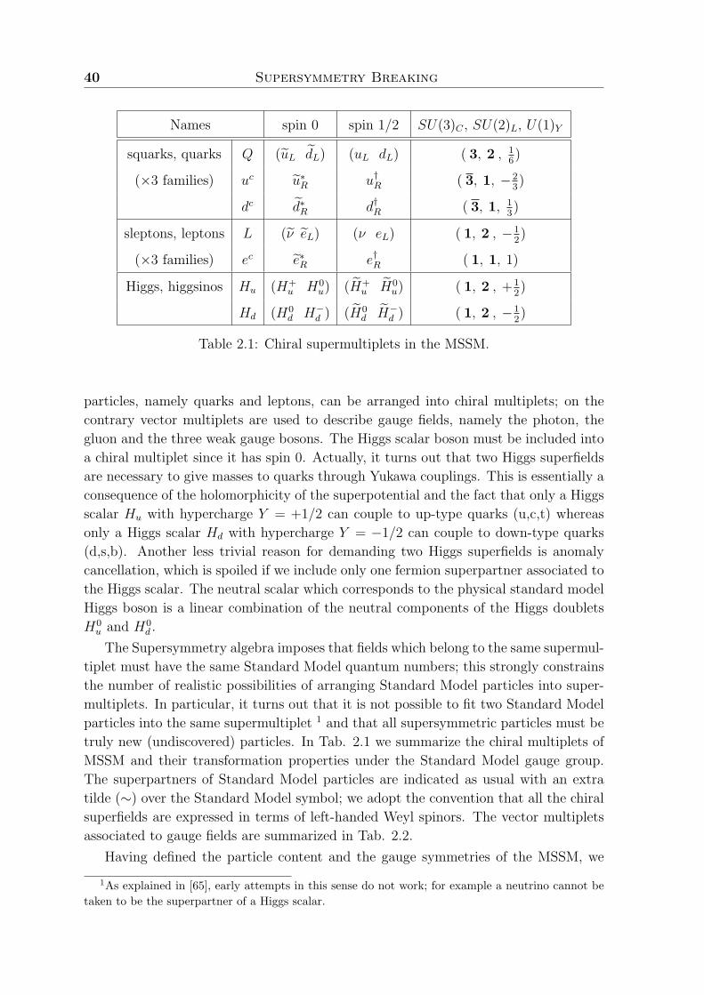
40 Supersymmetry Breaking
Names spin 0 spin 1/2 SU(3)C , SU(2)L, U(1)Y
squarks, quarks Q (uL dL) (uL dL) ( 3, 2 , 16)
(×3 families) uc u∗R u†R ( 3, 1, −23)
dc d∗R d†R ( 3, 1, 13)
sleptons, leptons L (ν eL) (ν eL) ( 1, 2 , −12)
(×3 families) ec e∗R e†R ( 1, 1, 1)
Higgs, higgsinos Hu (H+u H0
u) (H+u H0
u) ( 1, 2 , +12)
Hd (H0d H−d ) (H0
d H−d ) ( 1, 2 , −12)
Table 2.1: Chiral supermultiplets in the MSSM.
particles, namely quarks and leptons, can be arranged into chiral multiplets; on the
contrary vector multiplets are used to describe gauge fields, namely the photon, the
gluon and the three weak gauge bosons. The Higgs scalar boson must be included into
a chiral multiplet since it has spin 0. Actually, it turns out that two Higgs superfields
are necessary to give masses to quarks through Yukawa couplings. This is essentially a
consequence of the holomorphicity of the superpotential and the fact that only a Higgs
scalar Hu with hypercharge Y = +1/2 can couple to up-type quarks (u,c,t) whereas
only a Higgs scalar Hd with hypercharge Y = −1/2 can couple to down-type quarks
(d,s,b). Another less trivial reason for demanding two Higgs superfields is anomaly
cancellation, which is spoiled if we include only one fermion superpartner associated to
the Higgs scalar. The neutral scalar which corresponds to the physical standard model
Higgs boson is a linear combination of the neutral components of the Higgs doublets
H0u and H0
d .
The Supersymmetry algebra imposes that fields which belong to the same supermul-
tiplet must have the same Standard Model quantum numbers; this strongly constrains
the number of realistic possibilities of arranging Standard Model particles into super-
multiplets. In particular, it turns out that it is not possible to fit two Standard Model
particles into the same supermultiplet 1 and that all supersymmetric particles must be
truly new (undiscovered) particles. In Tab. 2.1 we summarize the chiral multiplets of
MSSM and their transformation properties under the Standard Model gauge group.
The superpartners of Standard Model particles are indicated as usual with an extra
tilde (∼) over the Standard Model symbol; we adopt the convention that all the chiral
superfields are expressed in terms of left-handed Weyl spinors. The vector multiplets
associated to gauge fields are summarized in Tab. 2.2.
Having defined the particle content and the gauge symmetries of the MSSM, we
1As explained in [65], early attempts in this sense do not work; for example a neutrino cannot betaken to be the superpartner of a Higgs scalar.
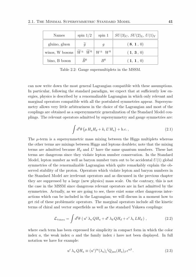
2.1. The Minimal Supersymmetric Standard Model 41
Names spin 1/2 spin 1 SU(3)C , SU(2)L, U(1)Y
gluino, gluon g g ( 8, 1 , 0)
winos, W bosons W± W 0 W± W 0 ( 1, 3 , 0)
bino, B boson B0 B0 ( 1, 1 , 0)
Table 2.2: Gauge supermultiplets in the MSSM.
can now write down the most general Lagrangian compatible with these assumptions.
In particular, following the standard paradigm, we expect that at sufficiently low en-
ergies, physics is described by a renormalizable Lagrangian in which only relevant and
marginal operators compatible with all the postulated symmetries appear. Supersym-
metry allows very little arbitrariness in the choice of the Lagrangian and most of the
couplings are obtained as a supersymmetric generalization of the Standard Model cou-
plings. The relevant operators admitted by supersymmetry and gauge symmetries are:∫d2θ(µHuHd + ki L
iHu
)+ h.c. , (2.1)
The µ-term is a supersymmetric mass mixing between the Higgs multiplets whereas
the other terms are mixings between Higgs and leptons doublets; note that the mixing
terms are admitted because Hd and Li have the same quantum numbers. These last
terms are dangerous since they violate lepton number conservation. In the Standard
Model, lepton number as well as baryon number turn out to be accidental U(1) global
symmetries of the renormalizable Lagrangian which quite remarkably explain the ob-
served stability of the proton. Operators which violate lepton and baryon numbers in
the Standard Model are irrelevant operators and as discussed in the previous chapter
they are suppressed by a large (new physics) mass scale. On the contrary, this is not
the case in the MSSM since dangerous relevant operators are in fact admitted by the
symmetries. Actually, as we are going to see, there exist some other dangerous inter-
actions which can be included in the Lagrangian; we will discuss in a moment how to
get rid of these problematic operators. The marginal operators include all the kinetic
terms of chiral and vector superfields as well as the standard Yukawa couplings:
LYukawa =
∫d2θ (uc λuQHu + dc λdQHd + ec λe LHd ) , (2.2)
where each term has been expressed for simplicity in compact form in which the color
index a, the weak index α and the family index i have not been displayed. In full
notation we have for example:
uc λuQHu ≡ (uc)ia(λu)ji Qjaα(Hu)β ε
αβ . (2.3)
42 Supersymmetry Breaking
In addition to these standard couplings it is possible to include the following dangerous
marginal operators:
Ldangerous =
∫d2θ ( dc λLQQQL+ ec λLLL LL+ λQQQu
cdcdc ) . (2.4)
The first two operators violate lepton number by one unit whereas the last operator
violate baryon number by one unit. As discussed in the first chapter, experimental
bounds on couplings which violate lepton and/or baryon number are quite stringent
and imply that they must be strongly suppressed with respect to other interactions.
The only natural way to achieve this suppression is to assume that these operators
are forbidden by some new global symmetry. Quite remarkably, all the dangerous
interactions can be excluded in an economical way by postulating just one new discrete
symmetry called R-parity or (matter parity); under this symmetry ordinary Standard
Model particles have charge +1 whereas their supersymmetric partners have charge
−1. At the superfield level, this can be achieved by the following transformation laws:
Φ(θ)→ ±Φ(−θ) V → +V (−θ,−θ) , (2.5)
where the minus sign in the transformations of chiral fields holds for L,Q, u, d while
the sign plus holds for Hu and Hd. Postulating R-parity conservation has two major
phenomenological signatures: in collider experiments, sparticles can only be produced
in pairs and the lightest supersymmetric particle (LSP) must be absolutely stable. This
last feature in particularly interesting since it provides a natural candidate for Dark
matter.
So far we have only discussed the structure of the SUSY-preserving part of the
MSSM Lagrangian but, as already discussed, supersymmetry breaking terms must be
included to construct a realistic model. The SUSY breaking Lagrangian contains the
most interesting operators from the point of view of phenomenology but, as we are going
to see in the following sections, it turns out to be the major source of arbitrariness in
the MSSM.
2.2 The Hidden Sector Paradigm and Soft SUSY
Breaking
It is obvious that supersymmetry cannot be an exact symmetry of nature because none
of the supersymmetric partner of the Standard Model particles has been observed so
far in collider experiments. Supersymmetric particles must have a mass larger than
∼ 100GeV in order to be consistent with the experimental bounds; however, as we
discussed in the previous chapter, their mass cannot exceed too much the TeV range
if we expect that supersymmetry is the mechanism that is responsible for the natural
stabilization of electroweak scale. Any satisfactory supersymmetric extension of the
Standard Model must then include a supersymmetry breaking sector which naturally
2.2. The Hidden Sector Paradigm and Soft SUSY Breaking 43
explains the non-observation of supersymmetric particles and which is consistent with
all the experimental bounds.
It is natural to try to construct a model in which supersymmetry is broken by
tree-level effects and communicated to MSSM fields by renormalizable interactions; as
an obvious analogy we can take the SU(2)× U(1) electroweak symmetry of the Stan-
dard Model whose breaking is triggered by the Higgs field v.e.v. and transmitted to
fermions through Yukawa interactions and to vector bosons through gauge interactions.
However, as anticipated, there exists a major difference between electroweak and su-
persymmetry breaking which prevents us to push this analogy any further. Indeed, in
supersymmetric models some non-trivial constraints associated to the supertrace for-
mulas reviewed in the previous chapter rule out any scenario in which supersymmetry
breaking is communicated to MSSM multiplets by tree level renormalizable couplings.
Let us analyze more in detail this aspect. The supertrace formula (1.67) for a renor-
malizable model and linearly realized symmetries (as the MSSM) reduces to:
sTr[m2] = 2 Tr[Ta ]Da . (2.6)
This trace formula holds separately for each set of conserved quantum numbers, namely
electric charge, color, baryon and lepton number; this is due to the fact the mass
matrices cannot have elements which connect particles with different values of these
quantum numbers. The trace of Ta vanishes automatically, unless Ta is a U(1) gener-
ator; moreover, the cancellation of the gravitational anomaly imposes that also all the
U(1) generators must be traceless. This finally implies that the supertrace is always
vanishing in any renormalizable supersymmetric model. This result is a disaster from
the phenomenological point of view since it implies that at least one of the superpar-
ticles must be lighter than its fermionic superpartner, and this is absolutely excluded
by experimental observations.
It is actually not too hard to overcome these difficulties, since the supertrace for-
mula (2.6) is only valid for renormalizable models and, furthermore, it does not take
into account radiative corrections. The standard paradigm to construct realistic su-
persymmetric scenarios is to postulate that the sector responsible for supersymmetry
breaking has no renormalizable tree-level couplings with the MSSM fields. Following
the standard conventions, we call this sector the hidden sector in order to distinguish
it from the observable sector which contains ordinary matter, gauge and Higgs fields
as well as their superpartners. Supersymmetry-breaking effects are communicated to
the MSSM supermultiplets by messenger fields, which interact with both observable
and hidden sector fields. In this scenario, the restrictions encountered in the minimal
setup can be avoided through a non-vanishing supertrace for the non-renormalizable
low energy effective theory which describes the dynamics of the observable sector fields.
The hidden sector paradigm allows to solve the severe constraints imposed by renor-
malizability in the trace formula but, as a draw back, it introduces a large amount of
arbitrariness since the field content of the hidden sector and the interactions responsible
for the transmission of SUSY-breaking effects are unspecified. Concerning the identi-
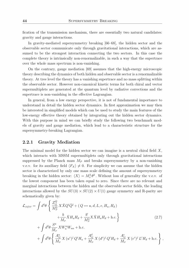
44 Supersymmetry Breaking
fication of the transmission mechanism, there are essentially two natural candidates:
gravity and gauge interactions.
In gravity-mediated supersymmetry breaking [66–68], the hidden sector and the
observable sector communicate only through gravitational interactions, which are as-
sumed to be the strongest interaction connecting the two sectors. In this case the
complete theory is intrinsically non-renormalizable, in such a way that the supertrace
over the whole mass spectrum is non-vanishing.
On the contrary, gauge mediation [69] assumes that the high-energy microscopic
theory describing the dynamics of both hidden and observable sector is a renormalizable
theory. At tree level the theory has a vanishing supertrace and no mass splitting within
the observable sector. However non-canonical kinetic terms for both chiral and vector
supermultiplets are generated at the quantum level by radiative corrections and the
supertrace is non-vanishing in the effective Lagrangian.
In general, from a low energy perspective, it is not of fundamental importance to
understand in detail the hidden sector dynamics. In first approximation we may then
be interested in simplified models which can be used to study the main features of the
low-energy effective theory obtained by integrating out the hidden sector dynamics.
With this purpose in mind we can briefly study the following two benchmark mod-
els of gravity and gauge mediation, which lead to a characteristic structure for the
supersymmetry-breaking Lagrangian.
2.2.1 Gravity Mediation
The minimal model for the hidden sector we can imagine is a neutral chiral field X,
which interacts with MSSM supermultiplets only through gravitational interactions
suppressed by the Planck mass MP and breaks supersymmetry by a non-vanishing
v.e.v. for its auxiliary field 〈FX〉 6= 0. For simplicity we can assume that the hidden
sector is characterized by only one mass scale defining the amount of supersymmetry
breaking in the hidden sector: 〈X〉 = M2S θ
2 . Without loss of generality the v.e.v. of
the lowest component has been taken equal to zero. Since there are no relevant and
marginal interactions between the hidden and the observable sector fields, the leading
interactions allowed by the SU(3) × SU(2) × U(1) gauge symmetry and R-parity are
schematically given by:
LSUSY/ =
∫d4θ
ZQi
M2P
XXQiQ + (Q↔ u, d, L, e,Hu, Hd )
+b
MP
XHuHd +b′
M2P
XXHuHd + h.c.
(2.7)
+
∫d2θ
Sa
MP
XWαaWaα + h.c.
+
∫d2θ
AuijMP
X (uc)j QiHu +AdijMP
X (dc)j QiHd +AeijMP
X (ec)j LiHd + h.c.
,
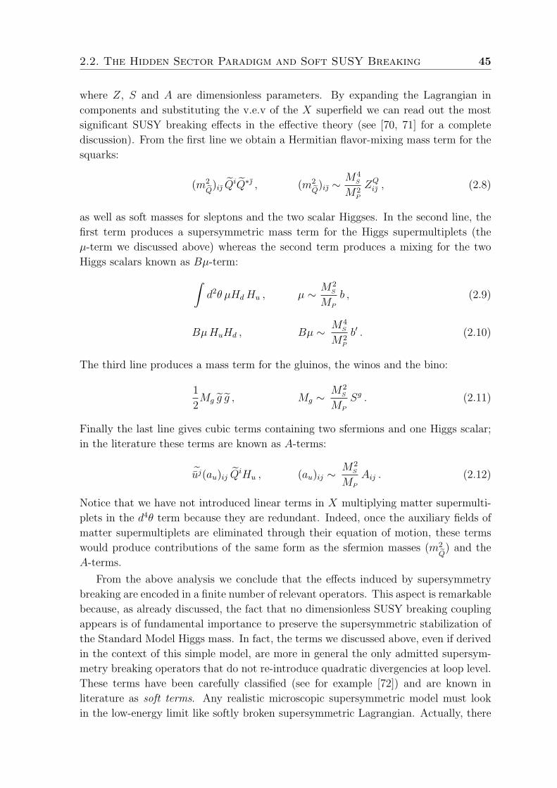
2.2. The Hidden Sector Paradigm and Soft SUSY Breaking 45
where Z, S and A are dimensionless parameters. By expanding the Lagrangian in
components and substituting the v.e.v of the X superfield we can read out the most
significant SUSY breaking effects in the effective theory (see [70, 71] for a complete
discussion). From the first line we obtain a Hermitian flavor-mixing mass term for the
squarks:
(m2eQ)i QiQ∗ , (m2eQ)i ∼
M4S
M2P
ZQi , (2.8)
as well as soft masses for sleptons and the two scalar Higgses. In the second line, the
first term produces a supersymmetric mass term for the Higgs supermultiplets (the
µ-term we discussed above) whereas the second term produces a mixing for the two
Higgs scalars known as Bµ-term:∫d2θ µHdHu , µ ∼ M2
S
MP
b , (2.9)
BµHuHd , Bµ ∼ M4S
M2P
b′ . (2.10)
The third line produces a mass term for the gluinos, the winos and the bino:
1
2Mg g g , Mg ∼
M2S
MP
Sg . (2.11)
Finally the last line gives cubic terms containing two sfermions and one Higgs scalar;
in the literature these terms are known as A-terms:
˜uj(au)ij QiHu , (au)ij ∼M2
S
MP
Aij . (2.12)
Notice that we have not introduced linear terms in X multiplying matter supermulti-
plets in the d4θ term because they are redundant. Indeed, once the auxiliary fields of
matter supermultiplets are eliminated through their equation of motion, these terms
would produce contributions of the same form as the sfermion masses (m2eQ) and the
A-terms.
From the above analysis we conclude that the effects induced by supersymmetry
breaking are encoded in a finite number of relevant operators. This aspect is remarkable
because, as already discussed, the fact that no dimensionless SUSY breaking coupling
appears is of fundamental importance to preserve the supersymmetric stabilization of
the Standard Model Higgs mass. In fact, the terms we discussed above, even if derived
in the context of this simple model, are more in general the only admitted supersym-
metry breaking operators that do not re-introduce quadratic divergencies at loop level.
These terms have been carefully classified (see for example [72]) and are known in
literature as soft terms. Any realistic microscopic supersymmetric model must look
in the low-energy limit like softly broken supersymmetric Lagrangian. Actually, there
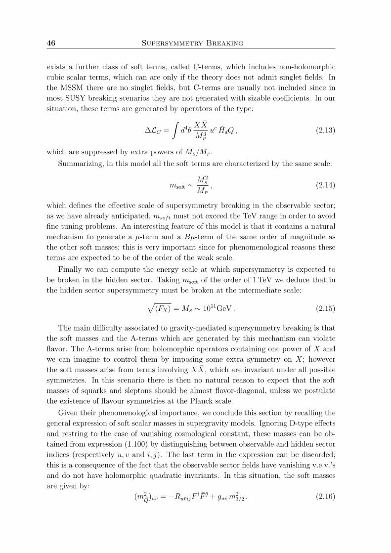
46 Supersymmetry Breaking
exists a further class of soft terms, called C-terms, which includes non-holomorphic
cubic scalar terms, which can are only if the theory does not admit singlet fields. In
the MSSM there are no singlet fields, but C-terms are usually not included since in
most SUSY breaking scenarios they are not generated with sizable coefficients. In our
situation, these terms are generated by operators of the type:
∆LC =
∫d4θ
XX
M3P
uc HdQ , (2.13)
which are suppressed by extra powers of MS/MP .
Summarizing, in this model all the soft terms are characterized by the same scale:
msoft ∼M2
S
MP
, (2.14)
which defines the effective scale of supersymmetry breaking in the observable sector;
as we have already anticipated, msoft must not exceed the TeV range in order to avoid
fine tuning problems. An interesting feature of this model is that it contains a natural
mechanism to generate a µ-term and a Bµ-term of the same order of magnitude as
the other soft masses; this is very important since for phenomenological reasons these
terms are expected to be of the order of the weak scale.
Finally we can compute the energy scale at which supersymmetry is expected to
be broken in the hidden sector. Taking msoft of the order of 1 TeV we deduce that in
the hidden sector supersymmetry must be broken at the intermediate scale:√〈FX〉 = MS ∼ 1011GeV . (2.15)
The main difficulty associated to gravity-mediated supersymmetry breaking is that
the soft masses and the A-terms which are generated by this mechanism can violate
flavor. The A-terms arise from holomorphic operators containing one power of X and
we can imagine to control them by imposing some extra symmetry on X; however
the soft masses arise from terms involving XX, which are invariant under all possible
symmetries. In this scenario there is then no natural reason to expect that the soft
masses of squarks and sleptons should be almost flavor-diagonal, unless we postulate
the existence of flavour symmetries at the Planck scale.
Given their phenomenological importance, we conclude this section by recalling the
general expression of soft scalar masses in supergravity models. Ignoring D-type effects
and restring to the case of vanishing cosmological constant, these masses can be ob-
tained from expression (1.100) by distinguishing between observable and hidden sector
indices (respectively u, v and i, j). The last term in the expression can be discarded;
this is a consequence of the fact that the observable sector fields have vanishing v.e.v.’s
and do not have holomorphic quadratic invariants. In this situation, the soft masses
are given by:
(m2eQ)uv = −RuvijFiF + guvm
23/2 . (2.16)
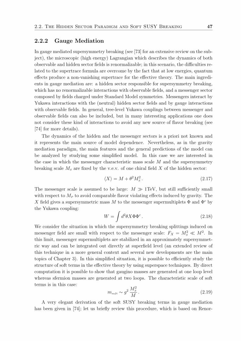
2.2. The Hidden Sector Paradigm and Soft SUSY Breaking 47
2.2.2 Gauge Mediation
In gauge mediated supersymmetry breaking (see [73] for an extensive review on the sub-
ject), the microscopic (high energy) Lagrangian which describes the dynamics of both
observable and hidden sector fields is renormalizable; in this scenario, the difficulties re-
lated to the supertrace formula are overcome by the fact that at low energies, quantum
effects produce a non-vanishing supertrace for the effective theory. The main ingredi-
ents in gauge mediation are: a hidden sector responsible for supersymmetry breaking,
which has no renormalizable interactions with observable fields, and a messenger sector
composed by fields charged under Standard Model symmetries. Messengers interact by
Yukawa interactions with the (neutral) hidden sector fields and by gauge interactions
with observable fields. In general, tree-level Yukawa couplings between messenger and
observable fields can also be included, but in many interesting applications one does
not consider these kind of interactions to avoid any new source of flavor breaking (see
[74] for more details).
The dynamics of the hidden and the messenger sectors is a priori not known and
it represents the main source of model dependence. Nevertheless, as in the gravity
mediation paradigm, the main features and the general predictions of the model can
be analyzed by studying some simplified model. In this case we are interested in
the case in which the messenger characteristic mass scale M and the supersymmetry
breaking scale MS are fixed by the v.e.v. of one chiral field X of the hidden sector:
〈X〉 = M + θ2M2S . (2.17)
The messenger scale is assumed to be large: M 1TeV, but still sufficiently small
with respect to MP to avoid comparable flavor violating effects induced by gravity. The
X field gives a supersymmetric mass M to the messenger supermultiplets Φ and Φc by
the Yukawa coupling:
W =
∫d2θXΦΦc . (2.18)
We consider the situation in which the supersymmetry breaking splittings induced on
messenger field are small with respect to the messenger scale: FX = M2S M2. In
this limit, messenger supermultiplets are stabilized in an approximately supersymmet-
ric way and can be integrated out directly at superfield level (an extended review of
this technique in a more general context and several new developments are the main
topics of Chapter 3). In this simplified situation, it is possible to efficiently study the
structure of soft terms in the effective theory by using superspace techniques. By direct
computation it is possible to show that gaugino masses are generated at one loop level
whereas sfermion masses are generated at two loops. The characteristic scale of soft
terms is in this case:
msoft ∼ g2 M2S
M. (2.19)
A very elegant derivation of the soft SUSY breaking terms in gauge mediation
has been given in [74]; let us briefly review this procedure, which is based on Renor-
48 Supersymmetry Breaking
malization Group (RG) techniques. At low energies E M , the dynamics of the
observable-sector fields can be described by a Wilsonian effective Lagrangian at the
renormalization scale µ M , defined by integrating out at the quantum level all the
modes with momentum larger than µ. The messenger fields can be completely inte-
grated out and, because of the non-renormalization of superpotential (see [75] for a
smart derivation of this result), the effective action is parametrized only by the wave
function Z(X, X, µ) and the holomorphic gauge kinetic functions Sg(X,µ):
Leff =
∫d4θ Z(X, X, µ)QQ+
∫d2θ Sg(X,µ)WαgW g
α + ... . (2.20)
Contrarily to the gravity mediation scenario, in this case the wave function Z is au-
tomatically flavor-diagonal, as required to avoid new sources of flavor violation. As
anticipated, the functional dependence of Sg and Z on the X superfield are obtained
by solving the RG equations for Sg(M,µ), Zi(M,µ) and by substituting back X to M
in a proper way. Gaugino and sfermion masses, as well as A-terms, can then be easily
found to be given by:
Mg(µ) = −1
2
∂ lnSg(X,µ)
∂ lnX
∣∣∣∣X=M
M2S
M, (2.21)
m2eQ(µ) = −∂2 lnZ(X, X, µ)
∂ lnX∂ ln X
∣∣∣∣X=M
M4S
M2, (2.22)
Ai(µ) =∂ lnZi(X,X
†, µ)
∂ lnX
∣∣∣∣X=M
M2S
M. (2.23)
From a technical point of view this method significantly simplifies the computation of
the soft terms and drastically reduces the number of Feynman diagrams to be com-
puted.
Without describing any further the details of the mechanisms which communicate
supersymmetry breaking effects to the observable sector, let us summarize what we
learnt from the previous examples. We have seen that the supertrace formula for-
bids scenarios in which the supersymmetry breaking sector interacts with the MSSM
supermultiplets through renormalizable interactions. This implies that the minimal
supersymmetric generalization of the Standard Model must be extended to include
a new non-standard sector whose physics is mostly unknown and is the main source
of arbitrariness in SUSY phenomenology. From a pragmatic point of view, we can
parametrize our ignorance by breaking explicitly SUSY in the MSSM through the
addition of soft terms that preserve the main features of SUSY as a solution of the
hierarchy problem. Any realistic microscopic theory which includes supersymmetry
must look in the infrared like a softly broken SUSY Lagrangian. In addition we have
seen that phenomenology imposes important constraints on the form and on the rel-
ative size of soft terms. The structure of soft terms is mostly related to the mecha-
nism by which supersymmetry breaking is communicated to the observable sector and
2.3. Hidden Sector in String-Inspired Models 49
several phenomenological constraints can be exploited to characterize the possible vi-
able scenarios. In our discussion we emphasized that the most stringent constraints
come from flavor physics. We have also stressed the fact that the structure of the
soft terms does not depend too much on the details of the hidden sector physics and
that the most relevant features of the soft SUSY breaking Lagrangian can be easily
captured by studying the simple models discussed above. This implies that from the
phenomenological point of view, very few low-energy constraints can be imposed on
the hidden sector physics. In other words, from the low-energy perspective, the hidden
sector looks like a “black box”and the only strong constraints that can be imposed on
the supersymmetry-breaking dynamics is demanding that the scalar potential for the
hidden sector fields admits a sufficiently long-lived metastable vacuum and that the
associated cosmological constant is positive and almost vanishing. Other constraints
come for instance from Big Bang nucleosynthesis [76], which is not compatible with
the existence of light scalars with masses smaller than 1 TeV.
In the last decades, many attempts have been made to describe the physics of the
hidden sector in the context of String Theory models. Indeed, as we are going to
discuss in the next section, a general feature of the low energy effective models derived
from String Theory is the existence of several neutral fields (moduli) which are natural
candidates to constitute the hidden sector responsible for supersymmetry breaking.
2.3 Hidden Sector in String-Inspired Models
In this section we present a qualitative review of the main topics in string phenomenol-
ogy which are relevant for our discussions (see [77] for a concise review in the spirit
of this section). The problematics we are going to discuss can be considered as the
principal motivation and inspiration for the studies presented in the next chapters.
Nevertheless, our results apply to more general contexts and, in practice, depend only
marginally on the arguments presented in this section.
At the present time, String Theory is the most accredited candidate for a truly
fundamental description of all interactions and, in particular, it is the most important
candidate theory to describe gravity at the quantum level. There exist five different
String Theories and all of them are consistent in 10 space-time dimensions (see [21, 22]).
A common feature of these theories is that the string spectrum contains a massless spin
2 particle, the graviton Gµν , a singlet massless scalar, the dilaton and antisymmetric
tensors of different ranks depending on the theory. In the low energy limit, obtained
by discarding all the massive excitations in the string spectrum, these theories are
described by ordinary supergravity models in 10D. Despite the uniqueness of the 10
dimensional theories, a large amount of arbitrariness is introduced when the six extra
dimensions are compactified (a la Kaluza-Klein) in order to obtain four-dimensional
theories. Most of the model dependence comes from the choice of the compactification
manifold; the requirement of having N = 1 supersymmetry in the four-dimensional
50 Supersymmetry Breaking
theory constrains the manifold to be a Calabi-Yau manifolds, which is a 6D Ricci flat
complex manifold.
The major problem in string phenomenology is that there exists a huge number of
topologically inequivalent Calabi-Yau manifolds (see for instance [22]) whose geometry
is controlled by the expectation values of moduli fields. These fields arise from the
dimensional reduction of the higher-dimensional graviton and other tensor fields; by
construction they are associated to the massless levels of the Kaluza-Klein tower. The
number of moduli that characterize each Calabi-Yau manifold is given by a set of
topological numbers known as Hodge numbers; they correspond to the number of
independent harmonic forms that can be defined on the compactification manifold.
There exist essentially two classes of moduli fields:
1. The Complex Structure moduli U , which characterize the shape of the compact-
ification manifold;
2. The Kahler moduli T , which control the size of the compact manifold.
Beside these fields and independently from the details of the compactification, each 4D
models contains the dilaton field S which fixes the string coupling.
We see that in String Theory there is then a twofold degeneracy on the “space” of
possible theories: the first one is a “discrete” degeneracy associated to the choice among
the topologically different Calabi-Yau manifold ,whereas the second one is a “contin-
uous” degeneracy, in the sense that, for each manifold, there is a set of massless fields
which can be freely varied and whose vacuum expectation values fix the shape and the
size of the compact manifold. This huge degeneracy can be visualized as a landscape
of string vacua [78] where each vacuum corresponds to a particular 4D model. In order
for String Theory to have any chance to be a realistic and predictive description of our
universe, it must incorporate a mechanism which explains how a particular vacuum
is selected or, in other words, how the compactification manifold is dynamically fixed.
This is one of the most challenging problems in string phenomenology and it is strongly
related to the problem of finding a natural mechanism to stabilize the moduli fields.
In the basic string constructions, the moduli fields U , T and S are massless fields
associated to flat directions of the scalar potential. In the last years, two main mecha-
nisms have been explored to generate a non-trivial dynamics for moduli fields and lift
the associated flat directions. Let us recall them.
1. Gaugino condensation (see for example [79–83]). Roughly speaking, in this
case, a non-trivial superpotential for certain moduli fields is generated by non-
perturbative effects due to the fact that they control also the gauge couplings
through the gauge kinetic function. If the gauge sector contains asymptotically-
free gauge interactions, gaugino condensation can naturally occur at the dynam-
ically generated scale Λ ∼ e−1/g. Through this mechanism a non perturbative
moduli-dependent superpotential a la ADS [84] (see also [85]) is generated.
2.3. Hidden Sector in String-Inspired Models 51
2. Flux compactication (see for example [86] for a detailed review). In this case a
tree-level moduli dynamics is generated by the addition of quantized background
fluxes. This mechanism stabilizes the moduli with a supersymmetric mass of the
order of the string scale, which is large with respect to the intermediate super-
symmetry breaking scale. One may then integrate out these heavy moduli and
work with a low energy supersymmetric effective theory describing the dynamics
of the remaining light moduli.
It is important to remark at this point that the quest for a natural mechanism
for moduli stabilization is essentially connected with the problem of finding a realistic
mechanism to break supersymmetry in the hidden sector; more precisely, it is natural
to expect that the same mechanism that is responsible for supersymmetry breaking
also produces a non-trivial dynamics for the light moduli fields. In many situations
that have been explored, none of the previous mechanisms is completely satisfactory
and in general, a combination of tree-level flux-induced dynamics and non-perturbative
effects is necessary to fully stabilize all the moduli and break supersymmetry. One fa-
mous example in this sense is the so called KKLT scenario [87]. The KKLT proposal
consists in a two steps moduli stabilization. In the first step fluxes are used to induce
a non-trivial potential for the dilaton S and the Complex Structure moduli U ; these
fields are stabilized with a supersymmetric mass which is assumed to be much larger
than the Kahler moduli masses. The author suggests that under these assumptions it
is possible to freeze S and U to their vacuum expectation values. The Kahler moduli T ,
on the other hand, remain unstabilized. In the second step, non-perturbative (gaugino
condensation) effects are invoked to stabilize T at a supersymmetric AdS minimum.
Finally, the authors use a brane sector to generate an uplifting (fine-tuned) poten-
tial that breaks supersymmetry and leads to a local minimum with a small positive
cosmological constant.
Many concerns have been raised regarding the validity of the KKLT procedure (see
for instance [88]). The weak point consists in the fact that the stabilization of S and U
fields is performed before including the non perturbative potential and without taking
into account the dynamics of T fields. The main question to be answered is whether one
is allowed to freeze the heavy moduli to their vacuum expectation values and decouple
them from the low energy dynamics. A more careful analysis would consist in properly
integrate them out in the complete supergravity theory describing the dynamics of all
the S, U and T fields.
This question is the main motivation for the study presented in Chapter 3 where,
in a completely general context, we discuss under which conditions it is possible to
integrate out heavy supermultiplets that are stabilized with large masses in order to
define an effective theory for the light modes. This problem is well understood in
the rigid limit whereas, as we will see, a more careful analysis is necessary in the
supergravity case. The importance of effective theories is evident in many research
fields in physics; in the case of moduli stabilization however it seems really crucial,
52 Supersymmetry Breaking
since it represents a fundamental tool to deal efficiently with the may moduli fields
that arise in most of the string compactification scenarios.
The physics of the hidden sector in string-inspired supergravity models is also the
main motivation for the second topic we are going to discuss in the forthcoming chapters
which, as anticipated, is metastability. The “continuous” degeneracy of string vacua
that we discussed above can be faced with the use of effective field theories; however
the “discrete”degeneracy associated to the choice among topologically different com-
pactification manifolds needs some new and more refined tool to be investigated. In
Chapter 4 we will derive some general criteria that allow to establish whether a su-
pergravity model can admit realistic metastable vacua depending on the geometrical
properties of the associated scalar (Kahler) manifold. In general, the geometry of the
scalar target space is completely determined by the details of the compactification and
having a model-independent procedure to discriminate among different compactifica-
tion scenarios can be very helpful.
Chapter 3
Supersymmetric Effective Field
Theories
Low-energy effective field theories are a very useful tool which can be used to simplify
the study of complicated systems involving a large number of fields. Whenever there
exist large hierarchies in the mass spectrum one expects that the dynamics of the
light degrees of freedom can be more efficiently described by a simpler low-energy
macroscopic Lagrangian in which heavy modes do not explicitly appear and the small
effects induced by their dynamics are encoded into a new set of effective parameters.
In string-inspired supersymmetric models, effective field theory is a particularly useful
instrument to study the dynamics of moduli fields of the hidden sector. In that case, the
large number of fields makes it prohibitive to study analytically the vacuum structure
in the microscopic Lagrangian and a drastic simplification is required.
In this chapter we address the problem of how to construct low-energy effective the-
ories in globally and locally supersymmetric theories by integrating out heavy fields.
We consider general non-linear sigma models with chiral and vector multiplets and we
study under which conditions the low-energy effective theory turns out to be approxi-
mately supersymmetric. These conditions translate into the requirements that all the
derivatives, fermions and auxiliary fields should be small in units of the heavy mass
scale. They apply not only to the matter sector, but also to the gravitational one if
present, and imply in that case that the gravitino mass should be small. We then argue
that in this limit the ordinary procedure, which applies also for non-supersymmetric
models, can be replaced by a more efficient one which consists in integrating out heavy
fields directly at the superfield level. We show how to determine the unique exactly
supersymmetric theory that approximates this effective theory at the lowest order in
the counting of derivatives, fermions and auxiliary fields, by working both at the su-
perfield level and with component fields. As a result we give a simple prescription for
integrating out heavy superfields in an algebraic and manifestly supersymmetric way,
which turns out to hold in the same form both for globally and locally supersymmetric
theories, meaning that the process of integrating out heavy modes commutes with the
53
54 Supersymmetric Effective Field Theories
process of switching on gravity. More precisely, for heavy chiral and vector multiplets
one has to impose respectively stationarity of the superpotential and the Kahler poten-
tial. We will mainly discuss the tree-level (classical) integration of heavy fields; a brief
qualitative analysis of quantum corrections is discussed in the last part of the chapter.
This chapter is based on our paper [1].
3.1 Integrating Out Heavy Fields: General Setup
In supersymmetric theories there exist essentially two approaches to construct low-
energy effective theories by integrating out heavy fields. The superspace formalism
suggests that it should be possible to do this directly at the superfield level by solv-
ing the superfield equations of motion of the heavy multiplets. On the other hand,
working with the extended Lagrangian written in component fields, one is induced to
integrate each heavy field by separately solving the corresponding equations of mo-
tion, and in general this turns out to be a more involved procedure. The questions
we want to address in this chapter are then the following: are these two procedures
equivalent? Under which conditions is it possible to apply the superfield approach and
in which limit do the two effective Lagrangians coincide? To answer these questions
we need to discuss the possible scenarios that may arise for the stabilization of heavy
modes. In general, the heavy fields will be stabilized at values implying a spontaneous
breakdown of supersymmetry, and the low-energy effective theory will consequently be
non-supersymmetric. In such a case, the best thing that one can do is to proceed in
the same way as for ordinary effective theories. In particular, at the leading order in
derivatives the effective theory is obtained by determining the heavy fields in terms of
the light ones by requiring stationarity of the potential with respect to the heavy fields.
However, it may happen that the heavy fields are stabilized in an approximately super-
symmetric way, with vacuum expectation values that break only very little or not at all
supersymmetry. In this limit we expect that the manifestly supersymmetric approach
in superfields differs from the actual effective theory only by small effects. It is then
of general interest to understand more precisely under which conditions such a situa-
tion can arise and to develop a systematic procedure to construct the supersymmetric
low-energy effective theory.
The case of theories with global supersymmetry is well understood, both for chi-
ral [84, 89] and vector multiplets [90–92], but we will nevertheless review it in some
detail. In this case one arrives very naturally at a simple procedure allowing to inte-
grate out heavy superfields directly at the superspace level, and thus in a manifestly
supersymmetric way. One particularly relevant situation where this procedure can be
very usefully employed is that of supersymmetric Grand Unified Theories, with a high
scale of gauge symmetry breaking yielding large masses for several fields [90, 91]. The
case of supergravity theories, on the other hand, seems to be less understood, and the
main aim of this chapter is to clarify how one should proceed in that case. For chiral
3.1. Integrating Out Heavy Fields: General Setup 55
multiplets, the question has been investigated some time ago in [93], and some diffi-
culties seem to appear, whereas for vector multiplets the situation seems to be simpler
[92] (see also [94, 61, 95]). We will however show that also in this case under suitable
conditions one arrives at a simple prescription for integrating out heavy superfields in a
manifestly supersymmetric way. The main result of our analysis is that the procedure
to integrate out heavy multiplets in supergravity is the same as in the rigid case once
the condition of small gravitino mass is satisfied.
The basic reason why gravity does not affect the way in which one integrates out
heavy fields at the leading order in the low-energy expansion is due to the fact that
when requiring also gravity to be described at the two-derivative level, its couplings
are essentially fixed. This is true in general, for any theory with fields of spin 0, 1/2
and 1, independently of whether it is supersymmetric or not. It can be understood
through the following argument. A generic two-derivative theory without gravity is
entirely parametrized by a potential V and some wave-function factors Z defining
the kinetic terms, which are functions of the fields. To get the effective theory at
the two-derivative level, one can then integrate out the heavy fields ξh by using as
equations of motion ∂hV = 0 and completely neglecting space-time derivatives. As
a matter of fact, this correctly determines not only the effective potential, but also
the effective wave-function factors. The reason is that the corrections to the equation
∂hV = 0 involve derivatives of the fields. Their effect can then be neglected in the wave
function Z, since this would give terms with more than two derivatives in the action.
It is easy to see that their effect can also be neglected in V . The reason for this is
that only the leading linear effect can produce a term with two or less derivatives, but
this term is proportional to ∂hV evaluated on the approximate solution and therefore
vanishes. When switching on gravity, the potential and kinetic terms get covariantized
in a unique way, and the only new allowed term is an Einstein-Hilbert kinetic term
for gravity, multiplied by a function Ω of the fields. One can then repeat exactly the
same reasoning as without gravity, treating Ω in a similar way as Z, and arrive again
to the conclusion that one can use the simple equation ∂hV = 0 to define the effective
theory at the two-derivative level. The case of supersymmetric theories is then just a
special case of this. For heavy chiral multiplets Φh, the Kahler potential K plays a role
similar to Z, whereas the superpotential W corresponds essentially to V . For heavy
vector multiplets V x, it is instead the gauge kinetic function H that plays the role of
Z and the Kahler potential K that plays the role of V . In the case where such heavy
chiral and vector superfields are stabilized in an approximately supersymmetric way,
the analogs of the equation ∂hV = 0 turn then out to be respectively ∂hW = 0 and
∂xK = 0. For exactly the same reasons as before, these equations allow to correctly
compute not only the effective potential but also the wave function factors, and turn
out to be valid also in the presence of gravity. The only assumption behind this is that
gravity can be treated at the two-derivative level, and we shall see that this implies
that the gravitino mass should be small.
As anticipated in the previous chapter, the study we are going to present is partic-
56 Supersymmetric Effective Field Theories
ularly relevant in the context of the effective supergravity description of string models,
where some of the moduli fields may be stabilized in a supersymmetric way with a
large mass, like for example in the scenarios of [96, 87]. There has been some debate
on the circumstances in which it is justified to freeze such heavy moduli to constant
values [88, 97, 98] (see also [99, 100]), and although this issue has recently been settled
in [101–103], it is important to know the procedure to integrate them out in general.
3.1.1 The Derivative Expansion
In quantum field theories, one can get rid of heavy degrees of freedom at tree level
by integrating the equations of motion of the associated fields at leading order in
space-time derivatives. To illustrate this point and in order to better understand the
considerations done in the last part of the previous section, let us consider a simple non-
supersymmetric model containing two sectors of real scalar fields with a large hierarchy
in the mass spectrum. We indicate with φi the light fields, with φα the heavy ones and
with Mαβ the heavy-field mass scale:
L =1
2∂µφ
i∂µφi +1
2∂µφ
α∂µφα − V (φi, φα) , (3.1)
with
V (φi, φα) =1
2M2
αβ φαφβ + V (φi, φα) . (3.2)
At low energy we can solve perturbatively the equations of motion of the heavy fields:
φα = (+M2)−1αβ(−Vβ) ≈ −M−2αβ Vβ +O(φi
M2
). (3.3)
At leading order in space-time derivatives, we can replace φα in the microscopic La-
grangian (3.1) by :
φα → φα0 (φi) +O(φi
M2
), (3.4)
where φα0 (φi) is defined as the solution of the algebraic approximate equations of motion
M2αβ φ
β0 (φi) + Vα(φi, φα0 (φi)) = 0, which gives:
Vα(φi, φα0 (φi)) = 0 . (3.5)
The effective Lagrangian at the two-derivative level is then given by:
Leff =1
2Zij(φ
i) ∂µφi∂µφj − V (φi, φα0 (φi)) (3.6)
with
Zij(φi) = δij +
∑α
∂φα0∂φi
∂φα0∂φj
,∂φα0∂φi
= −∑β
V αβinv Vβi . (3.7)
The relation on the right side can be derived from (3.5) by taking a derivative with
respect to light fields and V αβinv denotes the inverse of Vαβ as a matrix. We see now
3.2. Integrating Out Heavy Chiral Multiplets in Global SUSY 57
explicitly that in the effective Lagrangian we are allowed to keep the corrections to
the wave function since the next-to-leading contributions of order O (φi/M2α) in the
scalar potential are proportional to Vα(φi, φα0 (φi)), which automatically vanishes.
The crucial point to take into account when dealing with supersymmetric low-
energy effective theories is that the usual expansion in number of derivatives does not
preserve order by order supersymmetry. Any truncation on the number of space-time
derivatives spoils then supersymmetry, unless some other measure is taken. This point
has already been discussed in Sections 1.3.1 and 1.3.2 where we studied the most
general non-renormalizable supersymmetric models in rigid SUSY; we have seen that
a restriction on the number of space-time derivatives implies also a restriction on the
number of fermions and auxiliary fields. As a matter of fact, this feature turns out to
be valid more in general also for SUGRA models and it is essentially due to the general
form taken by supersymmetry transformations.
When heavy multiplets are integrated out to define a low-energy effective theory
valid below a certain mass scale M , infinitely many terms with arbitrarily large num-
ber of auxiliary fields and fermions are generated and these terms are suppressed by
inverse powers of M . One may then decide to retain only those terms with the leading
number of space-time derivatives, auxiliary fields and fermions in order to preserve
supersymmetry, but this truncation is justified solely when not only derivatives but
also the auxiliary fields and fermions bilinears are small in units of M .
This means physically that the modes that are integrated out should not only be
heavy, but also be stabilized in a way that approximately preserves supersymmetry,
with small values for the fermions and auxiliary fields, implying in particular small
mass splittings. The supersymmetric low-energy effective theory defined in this way, by
truncating the total number of derivatives, fermion bilinears and auxiliary fields, is then
different from the standard low-energy effective theory, obtained by truncating only the
number of derivatives, and the two approximately coincide only in those regions of field
space where fermions and auxiliary fields are small. One can summarize this reasoning
by simply saying that a multiplet of fields can be integrated out in a supersymmetric
way only if it has a large supersymmetric mass.
In the following sections we study in detail how to supersymmetrically integrate out
heavy multiplets, both by working in components and by using the superfield approach.
3.2 Integrating Out Heavy Chiral Multiplets in
Global SUSY
Let us first consider the simplest case of a globally supersymmetric theory with light
chiral multiplets Φi and heavy chiral multiplets Φα, denoted collectively by ΦI . As we
have seen in Section 1.3.1 the most general Lagrangian containing the leading number
58 Supersymmetric Effective Field Theories
of space-time derivatives is:
L =
∫d4θ K(ΦI , ΦI) +
∫d2θW (ΦI) +
∫d2θ W (ΦI) , (3.8)
where K and W are not allowed to depend on supercovriant derivatives Dα. It is useful
to define a weight n which counts the number of space-time derivatives n∂, auxiliary
fields nF and fermion bilinears nψ of each term in the component Lagrangian and which
is preserved by supersymmetry. More precisely, by inspection of the supersymmetry
transformations of chiral multiplets (1.16)-(1.18), we see that we can assign n[φI ] = 0
to scalar fields and n[∂µφI ] = 1 to their derivatives. In order for δψI to have a well
defined n, we then need to assign n[F I ] = 1 also to the auxiliary fields. Finally to
assign the correct weight to ψ we should observe that the expression for δφI implies
that the operator δ carries the same weight as ψI , or schematically n[δ] = n[ψI ]. Using
again the transformation law δψI , we deduce that 2n[ψ] = 1, which implies n[ψ] = 1/2.
By this analysis we are then led to define the following parameter:
n = n∂ +1
2nψ + nF . (3.9)
Using this definition, we see that restricting to a supersymmetric Lagrangian with at
most 2 space-time derivatives translate into requiring n 6 2. But this, as already
discussed, produces also a limitation on the number of spinor and auxiliary fields.
We will use this weight to establish which terms give the leading contributions in the
supersymmetric limit of the low energy effective theory.
To work at the superfield level, it is more useful to define a weight p which just
counts the number of supercovariant derivatives:
p =1
2nDα +
1
2nDα . (3.10)
By rewriting any integral on the superspace as supercovariant derivatives plus vanish-
ing boundary terms, we can verify that this definition is consistent with the previous
one, in the sense that to any term with a given weight p in superfield correspond terms
with weight n = p in components; more precisely, we see that all the terms coming
from the d4θ integral have n = 2 whereas all the terms coming from the d2θ integral
have n = 1. In superfield language, restricting to two-derivatives Lagrangians then
consistently translates in requiring p 6 2.
Superfield approach
Let us start by studying in detail how to supersymmetrically integrate out the heavy
multiplets using the superfield approach. The exact superfield equation of motion for
Φα is obtained by first rewriting the first term in eq. (3.8) as an F -term by making use
3.2. Integrating Out Heavy Chiral Multiplets in Global SUSY 59
of supercovariant derivatives, and then varying L with respect to the unconstrained
chiral superfield Φα. This yields:
Wα −1
4D2Kα = 0 . (3.11)
The presence of a large supersymmetric mass for Φα means that around the value Φα0
at which the superfield is stabilized, the superpotential W has a large second derivative
Wαβ(Φi,Φα0 ) setting the mass scale M . This implies that the first term in eq. (3.11)
dominates over the second and that, at leading order in 1/M , we can integrate out the
heavy chiral multiplets by replacing Φα in the microscopic Lagrangian (3.8) by:
Φα → Φα0 (Φi) +O
(D2Φi/M
), (3.12)
where Φα0 (Φi) is determined by the algebraic equation Wα(Φi,Φα
0 ) = 0 .
It turns out that the corrections O(D2Φ/M
)can be completely neglected in our
approximation, as the leading contributions that they would give to the effective action
would have p = 3. This statement is obvious for the terms coming from K, which gives
terms with p = 2 in the absence of extra supercovariant derivatives. For the terms
coming from W , which gives terms with p = 1 in the absence of extra supercovariant
derivatives, this is on the other hand due to the fact that the leading correction is
proportional to Wα, and therefore vanishes on the leading order solution. Summarizing,
one can thus integrate out the superfields Φα by using the simple chiral superfield
equation
Wα = 0 . (3.13)
This equation determines in an algebraic way the heavy chiral superfields in terms of
the light chiral superfields:
Φα = Φα0 (Φi) . (3.14)
The effective theory for the Φi is then obtained by plugging back this solution into K
and W . This yields:
Keff(Φi, Φı) = K(Φi, Φı,Φα0 (Φi), Φα
0 (Φı)) , (3.15)
W eff(Φi) = W (Φi,Φα0 (Φi)) . (3.16)
Component approach
It is instructive to rederive these results by using component fields. The Lagrangian
has the usual form L = T −V and it is given by expression (1.15). The kinetic part is
T = −KIJ
(∂µφ
I∂µφJ + iψJ σµDµψI), (3.17)
with DµψI = ∂µψ
I + ΓIMN∂µφMψN , and the potential is given by
V =−WIFI − WJ F
J +1
2WIJψ
IψJ +1
2WIJ ψ
IψJ
− KIJFIF J +
1
2KIJKF
IψJ ψK +1
2KJMNF
JψMψN − 1
4KIJP Qψ
IψP ψJ ψQ .
(3.18)
60 Supersymmetric Effective Field Theories
Recall that the capital indices run over all fields whereas we reserve i and α indices
to refer respectively to light and heavy fields. Recall also that the auxiliary fields are
actually determined by their algebraic equations of motion, and are given by:
F I = −KIJ(WJ −
1
2KJMNψ
MψN). (3.19)
We can now derive the exact equations of motion of Fα, ψα and φα. These corre-
spond to the θ0, θα and θ2 components of (3.11) and determine respectively the values
of the auxiliary fields Fα, the wave equation for ψα and the wave equation for φα. One
finds, without needing to use eq. (3.19), the following equations:
Wα +KαJ FJ − 1
2KαIJ ψ
IψJ = 0 , (3.20)
WαIψI +KαIJψ
IF J − 1
2KαIJKψ
I(ψJ ψK) + iKαJσµDµψ
J = 0 , (3.21)
WαIFI − 1
2WαIJψ
IψJ +KαIJFIF J − 1
2KαIJKF
IψJ ψK − 1
2KαJMNF
JψMψN
+1
4KαIJP Qψ
IψP ψJ ψQ +KαJφJ +KαJK∂µφ
J∂µφK = 0 . (3.22)
Under supersymmetry transformations, these equations get mapped into each other
and remain thus satisfied.
In the situation in which the fields φα and ψα have a large supersymmetric mass
M , there must be a quadratic term in W leading to a second derivative Wαβ of order
M . The equations of motion (3.21) and (3.22) for ψα and φα are then dominated by
the first terms, which involve second derivatives of W . Similarly, in the equation of
motion (3.20) for Fα, the first term is expected to dominate, since the other two do not
involve W at all. In the brutal limit in which one takes M → ∞ one would find that
φα is determined by the condition Wα(φα) = 0 whereas ψα and Fα vanish. However,
this brutal approximation does not preserve supersymmetry. One therefore needs to
look at the subleading terms and check which ones should be kept in order to get a set
of equations that is supersymmetric. The appropriate criterion to do so is related to
the counting of the total number n of derivatives, fermion bilinears and auxiliary fields.
Indeed, in order to obtain an effective theory with n ≤ 2, each of the equations used to
integrate out the heavy fields in terms of the light ones should involve terms with the
same minimal value of n. Looking at eqs. (3.20)–(3.22), it is easy to see that the terms
depending on W have a value of n that is one unit less than the terms depending on
K and are therefore the dominant ones. One may then drop all the terms involving K
and find the following set of approximate equations:
Wα = 0 , (3.23)
WαIψI = 0 , (3.24)
WαIFI − 1
2WαIJψ
IψJ = 0 . (3.25)
3.2. Integrating Out Heavy Chiral Multiplets in Global SUSY 61
It is easy to check that these are now exactly supersymmetric. More precisely, under
supersymmetry transformations each equation transforms into a combination of its
space-time derivative and one of the other equations. These equations are in fact the
non-trivial components of a chiral superfield equation, which is nothing but eq. (3.13).
The first of them is now understood as determining φα, the second ψα and the third
Fα. The bottom line is that the appropriate equation to be used to integrate out
the scalar fields is indeed the naive one, whereas for the fermion and auxiliary fields
supersymmetry forces us to keep some subleading terms suppressed by the mass scale
M .
Let us finally spell out more concretely the content of the three components (3.23)–
(3.25) of the superfield equation (3.13) by explicitly expressing heavy fields in terms of
the light ones. It is useful to introduce the following notation for the supersymmetric
masses of the heavy fields and the light fields, their mixings and ratios:
Mαβ = Wαβ , mij = Wij , µαi = Wαi , εαi = −M−1αβ µβi . (3.26)
The other relevant parameters are the cubic couplings in the superpotential involving
heavy chiral multiplets, namely:
λαij = Wαij , λαβj = Wαβj , λαβγ = Wαβγ . (3.27)
The first equation (3.23), compared to (3.20), states that the scalar components φα of
the heavy chiral multiplets must adjust to values compatible with the assumption that
all the ψI and F I vanish in first approximation:
φα0 (φi) : solution of Wα(φi, φα0 ) = 0 . (3.28)
The second equation (3.24) tells us instead that the heavy fermions ψα are not exactly
zero but proportional to the light ones, ψi, through a coefficient given by the ratio
between the supersymmetric mass mixing µ between light and heavy fields and the
mass M of the heavy fields:
ψα0 (φi, ψi) = −(M−1µ)αi ψi = εαi ψ
i . (3.29)
Finally, the third equation implies that the Fα are not exactly zero, but proportional
to the F i, plus some terms quadratic in the ψi, again through coefficients involving the
ratio between µ and M :
Fα0 (φi, ψi) = εαi F
i (3.30)
+1
2
(M−1αβλβij + 2M−1αβλβγi ε
γj + M−1αβλβγδ ε
γi εδj
)ψiψj .
In summary, we see that this procedure automatically keeps track of the fact that
the heavy superfields have small but yet non-vanishing fermion and auxiliary field
components. The effects of these suppressed components are in general relevant and
62 Supersymmetric Effective Field Theories
cannot be neglected. The final result is then a supersymmetric effective theory that is
accurate at leading order in ∂µ/M , ψI/M3/2 and F I/M2, but a priori not limited to
small φI/M .
We have checked in a variety of examples that the supersymmetric effective theory
defined by the superfield equation Wα = 0 and the standard effective theory defined
by the ordinary equation Vα = 0 do indeed approximately coincide under the above as-
sumptions. Focusing for concreteness on the scalar potential, the region in the space of
scalar fields φi where the two theories match is defined by the following two conditions:1
m(φi), µ(φi)M , F i(φi), Fα(φi)M2 . (3.31)
3.3 Integrating Out Heavy Chiral Multiplets in
Supergravity
Let us consider next the case of a locally supersymmetric theory with light chiral mul-
tiplets Φi and heavy chiral multiplets Φα, denoted collectively by ΦI , as well as the
gravitational multiplet. As anticipated in Section 1.4 we will work in the superconfor-
mal formalism; in this framework it is possible to rewrite as superspace integrals all the
relevant terms of the Lagrangian, which contain the couplings between the auxiliary
field Fφ and the matter and gauge fields. Schematically we can write:
L =
∫d4θ
(−3 e−K/3 ΦΦ
)+
∫d2 θW Φ3 + h.c. + gravity(eaµ, ψµ, Aµ) . (3.32)
The superspace part of the SUGRA Lagrangian turns out to be the most significant
one for our purposes and in our analysis we will focus on it. The omitted terms, as we
have already discussed in Chapter 1, are completely fixed by covariance and for this
reason we will not keep track of them in our computations. In this formalism, the total
number n of derivatives, fermion bilinears and scalar auxiliary fields corresponds again
to half the number of supercovariant derivatives. Requiring n ≤ 2 amounts then to
work at leading order in space-time derivatives, auxiliary fields and fermion bilinears
in both matter and gravitational sector.
1Note that in general the whole supersymmetric mass matrix, including all the blocks m, µ andM , is field dependent. One has therefore to make sure that not only m but also the mixing termµ stay small compared to M (see also [104] regarding this point). One can however focus on thesupersymmetric part of the mass matrix, since the F I are independently assumed to be small.
3.3. Integrating Out Heavy Chiral Multiplets in Supergravity 63
Superfield approach
Working as in the rigid case, we can integrate out the heavy chiral multiplets by solving
their approximate equations of motion. The exact superfield equations are given by:
Wα −1
4D2(Kα e
−K/3Φ)Φ−2 = 0 . (3.33)
We assume that as before the presence of a large supersymmetric mass means that
around the value Φα0 at which the heavy superfields Φα are stabilized, the superpotential
W has a large second derivativeWαβ(Φi,Φα0 ) setting the mass scaleM . The equations of
motion are then dominated by the first term, and we can integrate out the heavy chiral
multiplets, at leading order in 1/M , by replacing Φα in the microscopic Lagrangian
(3.32) by:
Φα → Φα0 (Φi) +O
(D2Φi/M, D2Φ/M
), (3.34)
where Φα0 (Φi) is determined by the algebraic equation Wα(Φi,Φα
0 ) = 0.
As before, the sub-leading correctionsO(D2Φi/M, D2Φ/M
)can be neglected, since
they would give corrections with n > 2.2 The heavy chiral superfields can thus be
integrated out by using the same simple chiral superfield equation as in the rigid case,
namely
Wα = 0 . (3.35)
As before, the solution of this equation determines the heavy chiral fields in terms
of the light chiral fields:
Φα = Φα0 (Φi) . (3.36)
The effective theory for the Φi is then obtained by plugging back this solution into K
and W . This yields:
Keff(Φi, Φı) = K(Φi, Φı,Φα0 (Φi), Φα
0 (Φı)) , (3.37)
W eff(Φi) = W (Φi,Φα0 (Φi)) . (3.38)
Notice now that, as discussed in Section 1.4, the microscopic theory involving all
the fields has a Kahler symmetry acting as (Φ, K,W ) → (Φ eY/3, K + Y + Y ,We−Y ),
where Y (ΦI) is an arbitrary holomorphic function of the matter chiral superfields.
On the other hand, the superfield equation (3.35) defining the effective theory is not
manifestly invariant under such a transformation for generic Y . More precisely, it is
invariant if Y depends only on the Φi, corresponding to Kahler transformations within
the effective theory. But it is not invariant if Y depends also on the Φα. The reason
for this is that we have assumed in our derivation that the large mass scale M of the
heavy fields is associated only with a large quadratic term in W , and no large term in
K. This is clearly a gauge-dependent assumption and it selects a restricted subclass of
2A similar reasoning has also been used in [102, 103] in the special case of effective theories de-scribing string models with fluxes.
64 Supersymmetric Effective Field Theories
Kahler gauges, which is particularly well-suited to work out the effective theory.
One may wonder at this point whether it is really justified to neglect supercovari-
ant derivatives acting on the compensator, and try to see what is the outcome when
one keeps such terms and neglects only those where supercovariant derivatives act on
the other chiral superfields. Proceeding in this way, eq. (3.33) would not reduce to
eq. (3.35), but rather to
Wα −1
4Φ−2Kαe
−K/3D2Φ = 0 . (3.39)
In order to get rid of the dependence on the compensator, one can now use the exact
superfield equation of motion of Φ. From the Lagrangian (3.32), one finds that this
equation of motion is given by
W +1
4D2(e−K/3Φ
)Φ−2 = 0 . (3.40)
For the same reasons as before, all the terms involving supercovariant derivatives acting
on K can certainly be neglected. However, one should keep the terms where the
supercovariant derivatives act on the compensator. Eq. (3.40) then becomes
−1
4D2ΦΦ−2 = eK/3W . (3.41)
Plugging this relation back into eq. (3.39) allows finally to eliminate completely the
dependence on the compensator, and the final equation simply reads:
Wα +KαW = 0 . (3.42)
This equation can also be derived in a more direct way by choosing from the beginning
a Kahler gauge defined by Y = lnW . In this way one does not need to use the
compensator equation of motion, but the derivation still implicitly assumes that W 6= 0
and D2Φ 6= 0. More in detail, from the Lagrangian (1.94) we can derive the exact
superfield equation of motions for the heavy superfields:
D2(Gα e−G/3Φ) = 0 . (3.43)
By keeping only the term in which the supercovariant derivative acts on the compen-
sator superfield we obtain:
Gα e−G/3D2Φ = 0 , (3.44)
which is equivalent to (3.42) if the above-mentioned assumptions are satisfied.
Notice that eq. (3.42) reduces to the equation Wα = 0 in the rigid limit, and is
moreover manifestly invariant under Kahler transformations. However, a closer look
shows that it cannot possibly be the correct equation. An obvious problem is that it is
a vector and not a chiral superfield equation. This means that it cannot be solved as a
superfield equation by just setting the Φα to some functions of the Φi, due to the fact
3.3. Integrating Out Heavy Chiral Multiplets in Supergravity 65
that there are more component equations than component fields. On the other hand,
the original exact equation of motion (3.33) for Φα is chiral, and it is by dropping only
part of the terms involving supercovariant derivatives that one arrives at an equation
which is no longer chiral. Thus, the new equation must somehow also be approximately
chiral, meaning that only its chiral components should really be significant, the non-
chiral ones being approximately satisfied in an automatic way. This means that the
equation Wα + KαW = 0 cannot be used as an exact equation to define a manifestly
supersymmetric approximate version of the low-energy effective field theory, and that
the appropriate equation should instead be Wα = 0, as already argued. Through
this argument, which clarify the problems raised in [93], we have moreover learned
that neglecting terms involving supercovariant derivatives acting on the compensator
amounts to neglect W compared to M , i.e. to have approximately
W ' 0 . (3.45)
This equation should however not be imposed as an exact superfield equation as it
comes from a reasoning on the compensator superfield Φ, for which most of the compo-
nents can be gauged away. More precisely, in the formulation where the superconformal
symmetry is gauge-fixed to the super Poincare symmetry, only the lowest component
of this equation, corresponding to the equation coming from the auxiliary field of the
compensator (3.40), should be considered. Finally, it should also be emphasized that
although W must be neglected in the equation that is used to integrate out the Φα, one
should a priori not neglect terms involving W in the Lagrangian where the solution for
the Φα is substituted to obtained the effective theory for the Φi.
The crucial point behind this extra difficulty that one encounters in the gravitational
case is that space-time derivatives and supersymmetry-breaking auxiliary fields must
be small also in the gravitational sector. This brings up a new condition that needs to
be fulfilled in order to be in the situation in which an approximate two-derivative super-
symmetric low-energy effective theory is expected to exist: the compensator auxiliary
field Fφ should be much smaller than M :
Fφ M . (3.46)
Once all the other auxiliary fields F I are also assumed to be small, F I M2, this
condition implies that:
1. the gravitino mass (and therefore W ) is small, m3/2 M ;
2. the cosmological constant is small, VS M4.
The first statement is justified by the fact that m3/2 turns out to be a linear combi-
nation of F I and Fφ auxiliary fields; to see this we can use the equation of motion
of Fφ evaluated at the vacuum, which can be derived as the lowest component of the
superfield equations (3.40). We then obtain:
m3/2 = |W | eK/2 =
∣∣∣∣ e−K/6 Fφ − 1
3KIF
I
∣∣∣∣M . (3.47)
66 Supersymmetric Effective Field Theories
The second statement can be verified by rewriting the scalar potential (1.95) in a more
suitable way:
VS = gi FiF − 3m2
3/2 M4 . (3.48)
The effect induced by Fφ 6= 0 is to produce a splitting ∆m among the masses
of fields belonging to the same multiplet; we understand then that the reason for
requiring Fφ to be small is twofold. In a flat background it can represent a genuine
supersymmetry breaking effect and then it should be small in order to not induce too
large mass splittings. On the other hand, when SUSY is unbroken, it represents the
expected mass splitting in an AdS background, which is proportional to the inverse of
the curvature radius, and we must require
∆m ∝ 1/RAdS M , (3.49)
in order to justify a two-derivative small-curvature approximation for the graviton. We
will discuss in more detail later on these aspects when we will study the role of Fφ on
mass splittings.
It should be finally emphasized that this further condition Fφ M (or equivalently
m3/2 M) can in general not be achieved in a natural way, but must instead be
implemented through an adjustment of parameters in the Lagrangian. Notice however
that for phenomenological applications it is anyhow necessary to eventually tune this
cosmological constant to a yet smaller value in the low-energy effective theory. This
step does therefore not represent a really severe restriction. Nevertheless, it is not
possible to define a locally supersymmetric two-derivative low-energy effective theory
below M without making sure that this condition is satisfied.
Component approach
One can derive the same results using component fields in the ordinary formulation of
supergravity. We will work in the Einstein frame defined by the gauge fixing (1.89) of
the Lagrangian (1.82); in this case we find it useful to reabsorb the factorized phase
associated to W through a field redefinition. In addition, since we are not interested
in keeping track of the fermionic couplings, we will set the spinorial component of the
compensator multiplet to zero. We finally have:
Φ = eK/6 · 1, 0, U . (3.50)
This gauge choice has the advantage of getting rid of the mentioned phase but has the
disadvantage that the component Lagrangian is not manifestly invariant under Kahler
transformations. As explained in [25] Kahler invariance is restored if Kahler transfor-
mations are accompanied by a redefinition of the gravitino and the chiral fermions. We
finally remark that, as before, we will discard the dependence on all the gravitational
fields except U .
3.3. Integrating Out Heavy Chiral Multiplets in Supergravity 67
With these assumptions, the Lagrangian has the usual form L = T − V , with a
kinetic term that is the same as in global supersymmetry,3
T = −KIJ ∂µφI∂µφJ , (3.51)
and a potential taking the following form:
V =− WIFIeK/2 − WJ F
JeK/2 − 3WUeK/2 − 3 W UeK/2
−(KIJ −
1
3KIKJ
)F IF J −KIF
IU −KJ FJU + 3UU . (3.52)
The auxiliary fields F I and U are determined by their algebraic equations of motion,
which give:
F I = −KIJ(WJ +KJW
)eK/2 , (3.53)
U =(
1− 1
3KIK
IJKJ
)WeK/2 − 1
3KIK
IJWJeK/2 . (3.54)
From these equations it follows that:
WeK/2 = U − 1
3KJ F
J , (3.55)
WIeK/2 = −
(KIJ −
1
3KIKJ
)F J −KIU . (3.56)
We can now derive the equations of motion of Fα and φα. These correspond to the
θ0 and θ2 components of the exact equations of motion after performing the supercon-
formal gauge fixing on the compensator. One finds:
WαeK/2 +
(KαJ −
1
3KαKJ
)F J +KαU = 0 , (3.57)
WαIFIeK/2 +
(KαIJ −
1
3
(KIKαJ +KJKαI
)−KαKIJ +
1
3KαKIKJ
)F IF J
+(KαI −KαKI
)F IU − 2KαJ F
JU +KαJφJ +KαJK∂µφ
J∂µφK = 0 . (3.58)
In order to arrive at this last equation, we have used the relations (3.56) and (3.55)
that follow from eqs. (3.53) and (3.54).
To define an approximate low-energy effective theory, we can now neglect in each of
these equations those terms which are subleading in the counting of the total number
n of derivatives and auxiliary fields. In this way we get:
Wα = 0 , (3.59)
WαIFI = 0 . (3.60)
3Note that the Kahler covariant derivative emerges only after taking into account the couplingsto the vector auxiliary field that remains in the gravitational multiplet after superconformal gaugefixing.
68 Supersymmetric Effective Field Theories
We recognize now that these equations correspond indeed to the θ0 and θ2 components
of the superfield equation (3.35) obtained in the superfield approach.
To check the effect of the compensator auxiliary field Fφ = eK/6U , one may re-do
the same analysis without considering it as an auxiliary field but rather as an ordinary
scalar field. This can be easily done by first eliminating the field U from the two
equations for φα and Fα by using its equation of motion U = WeK/2 + 1/3KIFI .
Using also eq. (3.53), and dropping then in (3.57) and (3.58) only terms that are
subleading in the total number of derivatives and matter auxiliary fields, one would
find the following two equations:(Wα +KαW
)eK/2 = 0 , (3.61)(
WαI +KαIW +KαWI
)F IeK/2 − 2KαJW F JeK/2 = 0 . (3.62)
These should correspond to the θ0 and θ2 components of eq. (3.42). As a matter of
fact, this is indeed the case if one discards the last term in eq. (3.62). This is related to
the fact that (3.42) is a vector superfield equation which is only approximately chiral
and has, as already argued, also some θ2 and θ2θ2 components that must somehow
be automatically satisfied within our approximations. Its θ2 component, in particular,
implies that the quantity KαJW F J should be discarded. Under this assumption, the
above equations correspond then indeed to the chiral components of eq. (3.42). As
already argued, this equation cannot be taken as an exact superfield equation, and
this shows up here through the fact that the above set of component equations is not
preserved by supersymmetry transformations.
Let us finally study a bit more in detail, as promised, the role of the compensator
auxiliary field in the mass splitting between scalars and pseudo-scalars. In the limit
in which all the F I and U are small, the only term that survives at second order in
the expansion of the scalar potential around the vacuum is the supersymmetric mass
eKWIP WJNKPN φI φJ . On the other hand, if we only discard F I and we assume that
U cannot be neglected we obtain:
Lmass = −(NIPK
PQNQJ − 2KIJ |U |2)φI φJ +
1
2NIJUφ
IφJ +1
2NIJ U φ
I φJ , (3.63)
where
NIJ = eK/2WIJ + (KIJ −KIKJ)U . (3.64)
The physical masses are then no-longer degenerate in pairs, but display now a splitting
between scalars and pseudo-scalars, of the order of the off diagonal elements NIJU in
eq. (3.63). As anticipated, if supersymmetry is unbroken and the background geometry
is AdS, the mass splittings coincide with those required by the supersymmetry algebra
in AdS space. U represents then a curvature scale and more precisely the inverse of the
radius RAdS of AdS. In this case one must require that the Compton wave length 1/M
of the heavy fields should be much smaller that this curvature length L, in order to be
3.3. Integrating Out Heavy Chiral Multiplets in Supergravity 69
able to integrate out these states in the small curvature approximation. This implies in
particular U M . If on the other hand supersymmetry is broken and the background
geometry is Minkowski, the mass splittings represent a soft supersymmetry breaking
effect. U corresponds then to an effective supersymmetry breaking scale. In this case
one must require that the square mass M2 of the heavy fields should be much larger
than the mass splittings of order MU and U2 arising in eq. (3.63). This implies again
U M . Notice finally that if the condition U M is not satisfied, it is impossible
for any light chiral multiplets to heave both its scalar and pseudo scalar components
with a mass much smaller than M , 4 and the gravitino is also not light.
The content of the superfield equation (3.35) is the same as the one displayed in
eqs. (3.28)–(3.30) for the rigid case. The first equation states again that the φα must
adjust to values compatible with the assumption that all the ψα and Fα vanish in first
approximation, whereas the second and the third equations tell that ψα and Fα must
actually have small but non-vanishing values. As before, these suppressed components
are important and cannot be neglected. The final result is then a supersymmetric
effective theory that is accurate at leading order in ∂µ/M , ψI/M3/2, F I/M2 and U/M ,
but again a priori not limited to small φi/M .
We have checked in a number of examples that the supersymmetric effective theory
defined by the superfield equation Wα = 0 and the standard effective theory defined by
the ordinary equations Vα = 0 do indeed approximately coincide under the assumptions
mentioned above. For the scalar potential, in particular, the region in the space of scalar
fields φi where the two theories match is now defined by three conditions:5
m(φi), µ(φi)M , F i(φl), Fα(φi)M2 , m3/2(φi)M . (3.65)
In this case, it is not possible to perform analytic checks. The reason for this is that the
validity of the approximation requires not only the F i(φi) to be small, but also U(φi)
(corresponding to m3/2(φi)) to be negligible as compared to the mass scale M . One has
then one more condition than scalar fields, and this makes it impossible to re-express
the deviation between the two effective potentials as a function of F i(φi) and U(φi)
instead of φi. This reflects the fact that, as already mentioned, there generically exists
a domain in field space where all the F i(φi) are small, but in order to have in addition
that also U(φi) is small in a non-empty portion of this domain, one needs in general to
adjust some coefficients in the theory. Nevertheless, we performed a numerical point-
by-point check for several non-trivial examples and verified that indeed our general
conclusions hold true.
4A point similar to this last observation was already made in [98].5The first two conditions are as before required to make sure that there is indeed a hierarchy
between the light and heavy eigenvalues of the full supersymmetric mass matrix. The last additionalcondition is, as already explained, equivalent to the condition U(φi)M .
70 Supersymmetric Effective Field Theories
3.4 Integrating Out Heavy Vector Multiplets in
Global SUSY
Let us consider again the case of global supersymmetry, but including both chiral
multiplets ΦI and vector multiplets V A, which we split into light ones V a and heavy
ones V x (we will use the latin indices a, b, c, .... for light vectors and x, y, w, z, .... for
heavy ones). For simplicity we restrict to Abelian gauge fields, but the generalization
to the non-Abelian case is straightforward. As we discussed in Section 1.3.2, the most
general Lagrangian with the leading number of space-time derivatives is given by (1.35),
which we rewrite here in a slightly different form for convenience:
L =
∫d4θ[K(Φ, Φ, V )
]+
∫d2θ[W (Φ) +
1
64HAB(Φ) D2DαV AD2DαV
B]
+ h.c. .
(3.66)
The new important aspect to take into account when vector multiplets are introduced
is the fact that the counting of the total number of derivatives, fermion bilinears and
auxiliary fields gets modified; this is essentially related to the fact that vector multiplets
have mass-dimension 0 rather than 1 and this implies that in the superfield Lagrangian
there may appear operators with a higher number of supercovariant derivatives. We
can naively generalize the weight n to include vector multiplets by assigning to AAµ , λA
and DA respectively n = 0, 1/2, 1; to the additional components CA, χA and NA arising
in non-Wess-Zumino gauges must then be assigned n = −1,−1/2 and 0 to preserve
supersymmetry. This counting guarantees that the minimal Lagrangian has still n 6 2
but it has two major disadvantage: first of all, it does not preserve gauge invariance
(as one can easily verify by looking for example at the gauge transformation of AAµor the covariant derivatives); second, it is not true anymore that to each superfield
expression with a fixed weight p correspond terms with n = p. Indeed, we can see
that the d4θ integral which has p = 2 produces also terms with n equal to 0 (e.g.
from KAB|θ=0(V AV B)|θ2θ2) and 1 (e.g. from KA|θ=0VA|θ2θ2). More remarkably, with
this definition the kinetic term for gauge fields has p = 4 but the associated terms
developed in components have n = 2. This raises then the question of whether one
should in this case keep subleading terms with a higher number of covariant derivatives
acting on chiral and vector superfields. We will see that it turns out that this is again
not necessary, but for a slightly less trivial reason than the previous case.
Let us start our analysis by first studying the integration of heavy chiral multiplets
in the presence of light vector multiplets, both in global and local supersymmetry. We
will finally concentrate on the integration of heavy vector multiplets .
Heavy Chiral Multiplets in Gauged Models
Before to start studying the integration of heavy matter fields in supersymmetric gauge
theories, let us briefly discuss how this can be done in non-supersymmetric models; this
analysis will be useful as a guideline for the supersymmetric generalization. Consider
3.4. Integrating Out Heavy Vector Multiplets in Global SUSY 71
for simplicity the following Abelian gauge theory with light complex scalar fields φi, a
light gauge vector Aµ and heavy scalar fields indicated by φα. The Lagrangian is given
by:
L = DµφI D∗µφI − 1
4F µνFµν − V (φ, φ) , with Dµ + iAµ . (3.67)
The equations of motion of the heavy fields are given by:
D2φα +∂V
∂φα= 0 . (3.68)
We want to integrate the heavy fields at tree level by solving their approximate equa-
tions of motions.
The new aspect that one has to consider at this point is the fact that a naive
truncation on the number of ordinary space-time derivatives spoils gauge invariance
in the low energy effective theory. What one can do in this case to preserve gauge
invariance is to perform a truncation on the number of covariant derivatives instead
of ordinary derivatives; one may then ask under which conditions the additional terms
involving gauge vectors can be safely discarded. It is easy to verify that such terms
are controlled by the ratio between the mass of the gauge vector and the heavy mass
scale of the scalar fields, which is assumed to be small in the region of validity of the
low-energy effective theory. In this situation one is then allowed to neglect subleading
corrections depending on covariant derivatives in the solution of (3.68) and heavy scalar
fields can be integrated out exactly as in the non-gauged case by solving the algebraic
equation Vα = 0.
The same analysis can now be generalized to supersymmetric models with heavy
chiral multiplets in the presence of light vectors multiplets. Working at superfield level,
the equations of motion for heavy chiral multiplets are:
Wα −1
4D2Kα(Φ, Φ, V ) +
1
64Habα(Φ) D2DβV aD2DβV
b = 0 . (3.69)
As we have already discussed in this chapter, in order to preserve supersymmetry in the
low-energy effective theory, we need to solve these equations perturbatively in the su-
percovariant derivatives. At leading order one obtains Φα = Φα0 +O(D2Φi/M, D2V/M),
where Φα0 is the solution of Wα = 0. It is easy to verify that the subleading terms in-
volving supercovariant derivatives acting on chiral superfields produce only terms with
n > 3 when substituted into the superfield Lagrangian (3.66); we can then reasonably
discard these terms in first approximation. On the contrary, as anticipated in the final
part of the previous subsection, subleading terms involving supercovariant derivatives
of vector superfields are more subtle since they may generate terms in the effective
Lagrangian with n 6 2 and should in principle be kept. On the other hand, discarding
only supercovariant derivatives of chiral superfields while keeping the ones of vector
superfields spoils the gauge invariance of the low-energy effective theory. Indeed, at the
leading order and keeping only supercovariant derivatives of vector superfields (3.69)
becomes:
Wα −1
4(KαabDV
aDV b +KαaD2V a) +O(D2Φi/M, D4V/M2) = 0 . (3.70)
72 Supersymmetric Effective Field Theories
The perturbative solution is:
Φα = Φα0 + Φα
1 aD2V a + Φα
1 abDVaDV b +O(D2Φi/M, D4V/M2) , (3.71)
where the coefficients of the sub-leading terms are found to be:
Φα1 a(Φ
i) =1
4M−1αβKβa , (3.72)
Φα1 ab(Φ
i) =1
4M−1αβKβab . (3.73)
One can verify that the supercovariant derivative part in expression (3.71) spoils gauge
covariance of the solution and when substituted back into the original Lagrangian it
breaks explicitly gauge invariance of the effective theory. However, exact gauge in-
variance is restored if one neglects also supercovariant derivatives of vector superfields;
from expressions (3.72) and (3.73) we discover that these terms can be consistently
discarded if one assumes that:6
|XIa | M . (3.74)
This corresponds to require, as in the non-supersymmetric case, that the gauge vectors
must have small masses in order for gauge invariance to be preserved in the low-energy
effective theory. When this extra condition is satisfied, the exactly supersymmetric
gauge invariant effective theory can be constructed as in the pure chiral case by solving
the algebraic equation Wα = 0 obtained from eq. (3.71) by neglecting also the leading
corrections in supercovariant derivatives of the vector superfields.
In the more general case in which the theory contains also heavy vector superfields,
one should first integrate them out and then integrate out heavy chiral fields following
the prescription that we have just described. Let us then pass to study how to properly
integrate out heavy vector multiplets.
Heavy Vector Multiplets in Global Supersymmetry
The integration of heavy vector superfields does not introduce new complications. Let
us start as usual by studying the case of non-supersymmetric Abelian gauge theories
and then generalize it to the supersymmetric case. Let us consider the same Lagrangian
(3.67), but this time assuming that all the scalar fields are light and all the vector
fields are assumed heavy. Since each gauge field is massive, it propagates one extra
degree of freedom and one real scalar becomes unphysical. One usually gets rid of this
unphysical mode by fixing the unitary gauge. We can however work without fixing the
gauge freedom and check that the unphysical mode is automatically decoupled in the
low-energy effective theory.
The equation of motion of Aµ is:
∂νFνµ + 2|φi|2Aµ + i (φi∂µφı − φı∂µφi ) = 0 . (3.75)
6 Use the fact that Kaα = 2i gIJ X Ja and Kabα = 4 gIJ∇αXI
(aXJb) .
3.4. Integrating Out Heavy Vector Multiplets in Global SUSY 73
At leading order in space-time derivatives, we can neglect the term involving the field
strength; the subleading corrections contain 3 derivatives and can be discarded. We
then see that there are no subtle contributions to be discussed in this case and the
solution of the approximate equation of motion is given by:
Aµ = −i(φi∂µφ
ı − φı∂µφi )2|φi|2
. (3.76)
The only non-trivial feature to discuss is the fact that when we substitute this solution
back we obtain a non-invertible effective wave function, which admits a zero mode:
Leff =1
2
(∂µφ
ı , ∂µφi) (P⊥ıj P‖ı
P‖ij P⊥i
) ( ∂µφj
∂µφ
), (3.77)
where
P⊥ıj = δıj −1
2
φı φj|φ|2
, P‖ij −1
2
φiφj|φ|2
. (3.78)
The direction associated to the vanishing eigenvalue of the kinetic mode is (φi, φı)
and it corresponds to the unphysical would-be Goldstone, which is automatically pro-
jected out.
The same analysis can now be generalized to supersymmetric models. For conve-
nience in this case we prefer however to fix the gauge symmetries associated to heavy
vector multiplets, even if as discussed this is not really necessary. The most conve-
nient type of gauge fixing is the one in which some charged chiral superfield is fixed
to some reference scale (the Fayet gauge discussed in Chapter 1). In such a gauge,
the corresponding vector multiplet becomes a general real vector multiplet, with all its
components being physical. This way of proceeding allows to integrate out the heavy
vector superfields at the superfield level. The exact superfield equations of motion for
the heavy vector superfields V x are obtained by first rewriting the last two terms of
the Lagrangian (3.66) as D-terms by dropping two supercovariant derivatives, and then
varying L with respect to V x. This gives:
Kx +1
8Dα(HxAD
2DαVA)
+1
8Dα
(HxAD
2DαV A)
= 0 . (3.79)
The presence of large supersymmetric mass for V x means in this case that around the
value V x0 at which it is stabilized, the Kahler potential K has a large second derivative
Kxy(Vx
0 ) proportional to M2. The first term in eq. (3.79) then dominates over the
others, and V x is approximately determined by the simple equation Kx(Vx
0 ) = 0.
The departure from this approximate solution is in this case found to be ∆V x0 ∼
O(D4V a/M2, D4Φm/M2), where Φm denotes all the chiral multiplets that have not
been frozen by gauge-fixing conditions. In our approximation, this correction can be
neglected, since it would contribute only terms with n ≥ 3. For the terms coming from
H, which already lead to terms with n = 2 without extra supercovariant derivatives,
74 Supersymmetric Effective Field Theories
this is obvious. On the other hand, for the terms coming from K, which can now lead
to terms with n = 1 due to the vector superfields, this is due to the fact that the
leading correction is proportional to Kx, which vanishes on the approximate solution.
Summarizing, one can thus integrate out the superfields V x by using the simple vector
superfield equation
Kx = 0 . (3.80)
This equation determines the heavy vector superfields as real functions of the light
vector superfields and the chiral superfields plus their conjugates:
V x = V x0 (V a,Φm, Φm) . (3.81)
The effective theory for the V a and Φm is then obtained by plugging back this solution
into the original Lagrangian. In the particular case in which there are no light vector
multiplets one needs to consider only K and W , and one finds:
Keff(Φi, Φı) = K(Φi, Φı, V x0 (Φi, Φı)) , (3.82)
W eff(Φi) = W (Φi) . (3.83)
In the case where there are also light vector multiplets, one can also get new effects
from the gauge kinetic terms. In particular, the effective gauge kinetic function is easily
found to be:
Heffab = Hab −HaxK
−1xyKyb −HbxK−1xyKxb +HxyK
−1xzK−1xwKzaKwb . (3.84)
As in the case of chiral multiplets, the components of the superfield equation (3.80)
have a simple interpretation. To spell it out, let us first notice that the supersymmetric
mass matrix for the heavy vector superfields, the light ones and their mixing are given
by:
M2xy = 2Kxy , m2
ab = 2Kab , µ2xa = 2Kxa . (3.85)
The other object that enters is the coupling between one heavy vector multiplet and
two chiral multiplets:
Qxi = −1
2Kxi . (3.86)
Notice next that eq. (3.80) makes sense in any gauge. In order to interpret its com-
ponents in physical terms, the most convenient choice is a supersymmetric gauge. In
this way, one finds that the real scalar component Cx must adjust its value in a way
compatible with the approximate vanishing of Dx, whereas the other components are
related to corresponding components of the light superfields through coefficients sup-
pressed by inverse powers of the heavy mass. One may also go to the Wess-Zumino
gauge to simplify the component expansion. The first few components of (3.80) imply
then restrictions on the charged chiral multiplets fields. In particular, their scalar fields
must adjust in such a way that the tadpole for Dx cancels, whereas their auxiliary fields
are subject to a linear relation corresponding to the gauge invariance of the superpo-
tential. The higher components of (3.80) imply on the other hand that the non-trivial
3.5. Integrating Out Heavy Vector Multiplets in Supergravity 75
components of the vector superfield can be re-expressed in terms of components of the
charged chiral-multiplets. In particular, one finds that
Dx = −(M−20 µ2
0)xaDa + (M−2
0 Q0)xi FiF . (3.87)
This equation coincides with the exact equation of motion of the complex partner of
the would-be Goldstone boson eaten by the gauge boson (see equation (1.53)). Notice
that the first term has n = 1 and is always relevant whereas the second gives n = 2
and can thus give a relevant contribution only in K.
3.5 Integrating Out Heavy Vector Multiplets in
Supergravity
Let us finally consider the case of local supersymmetry, but including both chiral
multiplets ΦI and vector multiplets V A that are split into light ones V a and heavy
ones V x. Using the superconformal superspace formalism, the requirement n ≤ 2
corresponds as before to simply neglect any dependence on supercovariant derivatives,
except the ones in the kinetic terms for the gauge fields. The theory can then again be
parametrized in terms of a real Kahler potential K = K(ΦI , ΦI , V A), a holomorphic
superpotential W = W (ΦI) and a holomorphic gauge kinetic function HAB(ΦI) [49,
105, 60]. The Lagrangian takes in this case the form
L =
∫d4θ(−3 e−K/3
)ΦΦ +
∫d2θWΦ3 +
∫d2θ W Φ3 (3.88)
+1
64
∫d2θ HAB D
2DαV AD2DαVB +
1
64
∫d2θ HABD
2DαVAD2DαV B .
As in the rigid case, we shall fix the local gauge symmetry associated to each heavy
vector superfield, and the most convenient way to do this is to set a charged chiral
superfield to some reference value. The exact superfield equations of motion for the
heavy vector superfields are then obtained as before, and read:
Kx +1
8eK/3(ΦΦ)−1
[Dα(HxAD
2DαVA)
+ Dα
(HxAD
2DαV A)]
= 0 . (3.89)
The presence of a large supersymmetric mass implies again that around the values
V x0 at which the heavy superfields V x are stabilized, the Kahler potential K has a
large second derivative Kxy(Vx
0 ) proportional to M2. The first term in eq. (3.89)
dominates then over the others, and V x is approximately determined by the equation
Kx(Vx
0 ) = 0. As before, the departure from this approximate solution is found to be
∆V x0 ∼ O(D4V a/M2, D4Φm/M2), and can be neglected. Summarizing, one can thus
integrate out the superfields V x by using the same simple vector superfield equation
as in the rigid case, namely
Kx = 0 . (3.90)
76 Supersymmetric Effective Field Theories
Note that this equation is automatically and trivially invariant under Kahler transfor-
mations, since these are not allowed to depend on the vector superfields.
The components of this superfield equation admit exactly the same interpretation
as in the global case. This makes sense as long as the auxiliary field of the compensator
is small, implying m3/2 M . In particular, eq. (3.87) still holds true, but comparing
it with the exact equation of motion of the complex partner of the would-be-Goldstone
mode eq. (1.123) (see for instance [61, 62, 64, 63] and also [94, 95]), one finds that it
agrees with it only in the limit where m3/2 M and also F i M , which are indeed
satisfied in our approximation.
3.6 Summary
In this chapter, we have addressed the general question of understanding under which
conditions it is possible to define a two-derivative supersymmetric low-energy effective
theory by integrating out a heavy superfield with mass M , and we defined a procedure
to explicitly construct it. We studied the cases of chiral and vector multiplets, both
in global and in local supersymmetry. Concerning the conditions for the existence of
such a theory, we have argued that one has to require that all the derivatives, fermion
fields and auxiliary fields should be small in units of M . In the global case, this
means ∂µ M on all the fields, ψI , λA M3/2 for the chiralini and gaugini, and
F I , DA M2 for the chiral and vector auxiliary fields. In the local case, one has in
addition to impose ∂µ M on all the gravitational fields, ψµα M3/2 for the gravitino
and U M for the gravitational scalar auxiliary field. This implies that M should
correspond to a supersymmetric mass, that comes from W for chiral multiplets and
from K for the vector fields. We have then shown that under the above conditions the
superfield equations allowing to integrate out heavy chiral and vector superfields Φα
and V x in terms of light chiral and vector superfields Φi and V a are respectively the
stationarity of the superpotential and the Kahler potential W and K:
∂αW (Φi,Φα) = 0
∂xK(Φi, Φı,Φα, Φα, V a, V x) = 0
⇒Φα = Φα
0 (Φi) ,
V x = V x0 (Φi, Φı, V a) .
(3.91)
The fact that these equations are exactly the same in globally and locally supersym-
metric theories is a consequence of the assumption that higher-derivative terms should
be negligible also in the gravitational sector. This implies that the gravitino mass
should be much smaller than the supersymmetric mass M of the superfield to be in-
tegrated out: m3/2 M . One is then in a situation where the coupling to gravity is
minimal and essentially dictated by the space-time symmetries, except for the Einstein
term, which can however be canonically normalized in a universal way by going to the
Einstein frame from the start. As a result, the operations of integrating in/out heavy
fields and switching on/off gravitational interactions commute. Exactly the same thing
3.6. Summary 77
is true also for a generic non-supersymmetric theory, where the two-derivative effective
theory can be deduced by integrating out the heavy fields by imposing stationarity of
the potential.
In general, integrating out heavy superfields induces relevant corrections to the dy-
namics of the light superfields, which cannot be ignored in many interesting situations.
In principle, to compute these corrections one simply needs to solve the superfield
equations (3.91), which is a simple algebraic problem. In practice this may however
be a non-trivial task, for example due to non-linearities or due to the proliferation of
fields. It is then of interest to understand in which cases the effect of integrating out
heavy superfields is trivial, in the sense that it is equivalent to freezing these to some
constant values independent of the light superfields. According to the above superfield
equations (3.91), we see that for chiral superfields this is the case when W is separable,
W = WL(Φi) + WH(Φα), which still allows for non-trivial heavy-light interactions in
K. On the other hand, for vector superfields one would need K to be separable (for
supersymmetric gauges), K = KL(Φm, Φm, V a) + KH(V x), which implies that there
are no heavy-light interactions at all since vector superfields are not allowed to appear
in W . Actually, as far as the effective potential is concerned, this still approximately
works even in the case where W or K respectively consist of a dominant term depend-
ing only on the heavy superfields and an other one depending also on the light ones but
suppressed by some small parameter ε, provided that the gravitino mass is at most of
the same order ε.7 The reason is that W and K are stationary with respect to the ap-
proximate solution for the heavy chiral and vector fields and corrections can thus arise
only at second order. This property was already derived in a different way in [101],
and further generalized in [106]. Notice however that there may be cases in which W
and/or K are not separable but can be made separable after a superfield redefinition.
In that case, the integration of heavy superfields will also be trivial, but only in the new
superfield basis. Using the original field basis, one would find non-trivial corrections
for the light field dynamics, but these clearly simply implement in an automatic way
the field redefinition to the clever basis of light fields. On the other hand, in a generic
effective theory a heavy field can be integrated out in a exactly trivial way only if the
potential V is separable, at least at the point where the heavy fields are stabilized. For
supersymmetric theories, to have such an exact trivialization one needs the stronger
conditions that both K and W are separable in the rigid case, and that K is separable
and W factorizable in the local case [107], again at least at the point where the heavy
fields are frozen [108, 99, 100].
As a final remark, let us emphasize that although the above results were derived at
the classical level, similar considerations apply also at the quantum level. In particular,
it is always true that superfields with large supersymmetric masses can be integrated
out at the level of superfields to define a two-derivative supersymmetric low-energy
effective action. Due to the non-renormalization theorem for W , these loop corrections
7Note that this generically implies that m3/2 ∼ m, which is a stronger condition than the restrictionm3/2 M that is needed to be able to define a supersymmetric effective theory.
78 Supersymmetric Effective Field Theories
affect only K. See for example [109] and [110] for explicit examples in globally and
locally supersymmetric theories.
Chapter 4
Vacuum Stability and Bound on
the Lightest Scalar
In this chapter we study some general criteria for the existence of metastable vacua
with spontaneously broken global supersymmetry in generic supersymmetric models
with local gauge symmetries. In particular we derive an absolute upper bound on the
mass of the lightest scalar field which depends essentially on the geometrical proper-
ties of the scalar manifold and its gauged isometries. This bound can be saturated
by properly tuning the superpotential and its positivity therefore represents a nec-
essary and sufficient condition for the existence of metastable vacua. It is derived
by looking at the subspace of all those directions in field space for which an arbi-
trary supersymmetric mass term is not allowed and scalar masses are controlled by
supersymmetry-breaking splitting effects. This subspace includes not only the direc-
tion of supersymmetry breaking, but also the directions of gauge symmetry breaking
and the lightest scalar is in general a linear combination of fields spanning all these
directions. We explicitly present analytic results for the simplest case of globally super-
symmetric theories with a single Abelian gauge symmetry. For renormalizable gauge
theories, the lightest scalar is a combination of the Goldstino partners and its square
mass is always positive. For more general non-linear sigma models, on the other hand,
the lightest scalar can involve also the Goldstone partner and its square mass is not
always positive. The generalization of this analysis to local supersymmetry does not
present new conceptual obstructions even though it appears to be more involved from
the technical point of view; we qualitatively discuss this topic at the end of the chapter.
This chapter is based on our paper [2].
4.1 General Criteria for Metastability
In Chapter 2 we have seen that there exist several phenomenological arguments con-
straining the structure of the soft masses and the mechanism by which supersymmetry
breaking effects are transmitted to the visible sector. On the contrary, the only simple
79
80 Vacuum Stability and Bound on the Lightest Scalar
constraints one can impose on the actual mechanism responsible for supersymmetry
breaking in the hidden sector are the metastability of the vacuum and the value of the
cosmological constant.1 Even though these constraints may appear to be weak, they
can be used to define some relevant criteria to discriminate among different scenarios
for hidden sector physics. The important aspect to take into account is the fact that
the structure of the mass matrices in supersymmetric models is strongly constrained
and the spontaneous breaking of supersymmetry allows to split the masses of bosons
and fermions but not to achieve totally arbitrary mass matrices. In general, these mass
matrices consist of a supersymmetric contribution that is common to all the states of a
multiplet plus a non-supersymmetric contribution splitting the masses of these states
within each multiplet.
The first source of constraints is that the various non-supersymmetric contributions
to the masses are correlated among each other. A simple consequence of these correla-
tions is expressed by the celebrated supertrace formula that we discussed in Chapter
1. When computing this quantity, the supersymmetric contributions to masses drop
out and the non-supersymmetric contributions combine into a remarkably simple result.
This then constrains to some extent the relative masses that can be achieved for bosons
and fermions and has, as we have seen, important implications in phenomenological
model building.
The second source of constraints, which is the most relevant for our discussion,
consists in the fact that some of the supersymmetric contributions to the mass ma-
trices are constrained by symmetry arguments. More precisely, there exist particular
directions in field space which are associated to supersymmetric masses that cannot be
made arbitrarily large; such directions are dangerous in the sense that supersymmetry
breaking effects can make them unstable. One important example is the supersymmet-
ric contribution to the mass of the Goldstino chiral multiplet which must vanish, since
the fermion of this multiplet is constrained by Goldstone’s theorem to have vanishing
mass. As a result, the two scalar partners of this fermion have masses that are en-
tirely controlled by splitting effects. Similarly, the supersymmetric contribution to the
mass of the vector multiplets is fixed by the expectation value of the Killing vectors,
since the vector boson masses arise through the Higgs mechanism. As a result, the
real scalar partner of each massive gauge boson has a mass that differs from the gauge
boson mass only by splitting effects, and this can also be viewed as the statement that
the would-be Goldstone chiral multiplet has a constrained mass in the supersymmetric
limit.
A remarkable consequence of this second class of constraints is that there exists
an upper bound on the mass of the lightest scalar, even if the superpotential is freely
tuned. More importantly, the direction associated to the lightest scalar is in general
not arbitrary and it belongs to the subspace spanned by the Goldstino and the Gold-
1Other constraint from cosmological arguments is the existence of viable inflationary trajectoriesensuring a “slow-roll” motion of the inflaton field. See for instance [111–114]. In this work howeverwe will not take into account this class of constraints.
4.1. General Criteria for Metastability 81
stone partners. This suggests that to establish whether a model can admit metastable
vacua breaking supersymmetry, it is not really necessary to study the whole scalar
mass matrix, since the relevant information concerning metastability is contained in
some special sub-blocks associated to the dangerous directions discussed above. In this
chapter we want to develop this idea to derive some general necessary and sufficient
conditions for the existence of metastable vacua in models in which the Kahler geom-
etry and the gauged isometries are fixed whereas the superpotential can be arbitrarily
varied in order to saturate the bound on the mass of the lightest scalar. This analysis
can be relevant for string-inspired supersymmetric models obtained by compactifica-
tion since, as we discussed in Chapter 2, the structure of the Kahler potential is in
general determined by the details of the compactification whereas the structure of the
superpotential is more difficult to be determined. Since a priori there exist a plethora
of different compactification manifolds which are admitted by String Theory, it is very
useful to have some general criteria to discriminate among scenarios with different
Kahler geometries independently of the form of the superpotential, and to be able to
characterize the possible geometries which allow for realistic vacua.
The case of theories with only chiral multiplets and no gauge symmetries is well
understood. What matters in this case is the two-dimensional sub-block of the scalar
mass matrix restricted to the two Goldstino partners. For renormalizable models, the
two eigenvalues of this matrix are equal and opposite, and the best situation that can
occur is that both vanish. This implies the presence of two pseudo-moduli fields with
vanishing mass, which actually represent flat directions of the classical potential with
peculiar properties [115, 116]. For more general non-renormalizable chiral non-linear
sigma-models, one similarly finds that the two eigenvalues are split around an aver-
age value that is fixed by the Riemann curvature of the Kahler manifold, and in the
best situation one has two scalars with identical masses given by this value [108, 117].
Similar results also hold in supergravity theories, and these give a useful guideline to-
wards the ingredients that are needed to achieve metastable de Sitter vacua in string
models [118, 119]. More precisely, in the case in which supersymmetry breaking is
dominated by chiral multiplets, the requirement of metastability and positivity of the
cosmological constant can be operatively translated into constraints on the parameters
of the theory and it is possible to implement a well-defined procedure to locally re-
construct a scalar potential which admits metastable de Sitter vacua (see [120]). The
idea of using metastability criteria to characterize supersymmetry breaking scenarios
in string-inspired models has been proven to be very powerful in many situations; for
instance, it has been applied to prove in a simple and sharp way the fact that su-
persymmetry breaking dynamics cannot be dominate by a single Kahler Modulus or
by the dilaton unless subleading corrections to the Kahler potential are considered
[121–123, 108]
The case of theories involving also vector multiplets and local gauge symmetries is
more complicated and less understood (see for example [124, 125]). As anticipated, one
should in principle look at a higher-dimensional sub-block of the scalar mass matrix
82 Vacuum Stability and Bound on the Lightest Scalar
that includes not only the two Goldstino partners but also the Goldstone partners. In
this case the complexity of the analysis increases with the number of generators of the
symmetry transformations and studying the relevant sub-blocks of the mass matrix
may turn out to be a non-trivial task as much as studying the whole mass matrix. It
has been argued in [61] that the presence of D-type in addition to F -type supersym-
metry breaking tends to alleviate the metastability condition which can be derived by
looking only at the Goldstino direction. But a full analysis including also the Gold-
stone partners was still missing and, in particular, it is not obvious that the improving
effects associated to gauge vectors can always be used to achieve metastability.
The purpose of this chapter is to perform a detailed study of the scalar mass matrix
of generic theories with rigid N=1 supersymmetry and local gauge symmetries, and to
derive an upper bound on the value of its lightest eigenvalue. The main improvement
that we aim to achieve compared to previous analyses is to obtain the strongest possible
bound, with the property that it should be possible to saturate it by adjusting only
the superpotential. To achieve this goal, we will need not only to consider the effect of
the vector multiplets on the two Goldstino partners, but also to include in the analysis
the Goldstone partners, and focus our attention on the full dangerous sub-block of the
scalar mass matrix for which supersymmetric effects are constrained. The aim of this
analysis is to show that in general situations the directions associated to the Goldstone
partners play a relevant role in discussing metastability.
4.2 Structure of the Scalar Mass Matrix
Let us consider a generic globally supersymmetric model with n chiral multiplets Φi
and k vector multiplets V a defined by the Lagrangian (1.35):
L =
∫d4θ[K(Φ, Φ, V )
]+
∫d2θ[W (Φ) +
1
4Hab(Φ)W aαW b
α
]+ h.c. . (4.1)
As we did in the previous chapters, we exclude for simplicity the possibility of non-zero
variations of the Kahler potential under gauge transformations. In particular, we thus
exclude Fayet-Iliopoulos terms. In the following, we shall also restrict for simplicity to
the special case where the gauge kinetic function Hab is constant, so that Habi = 0.
This does not represent a very big conceptual limitation, but it leads to a substantial
simplification of the theory. We shall on the other hand retain the possibility of having
a generic Kahler potential K and generic Killing vectors X ia defining the non-constant
matrices
Qaij = i∇jX
ia . (4.2)
The particular case of renormalizable gauge theories corresponds to choosing K =
δijΦiΦ, X i
a = −i TaijΦj and Qaij = Ta
ij, with constant T aij.
For later convenience, we shall furthermore introduce an arbitrary gauge coupling
constant g, although this could be reabsorbed in the normalization of Hab; this amounts
4.2. Structure of the Scalar Mass Matrix 83
to slightly modify some relevant expressions that we encountered in Section 1.3.2 and
in particular the relation following from gauge invariance:
X iaKi =
i
2g−1Ka , (4.3)
Kai = 2igXai , (4.4)
giXi[aX
b] =
i
4g−1f c
ab Kc . (4.5)
The values of the auxiliary fields F i and Da are fixed by their equations of motion and
read:
F i = −giW , Da = − 1
2habKb = ighabX i
bKi = −ighabX ıbKı . (4.6)
The vacuum energy V is still given by
V = giFiF +
1
2habD
aDb . (4.7)
The stationarity condition Vi = 0 implies that
∇iWj Fj + igXaiD
a = 0 . (4.8)
We recall the fact that contracting the stationarity conditions with the Killing vector
and taking the imaginary part one obtains a very useful relation constraining F and
D term, which in this case reads:
QaiFiF − 1
2g–1M2
abDb = 0 . (4.9)
Finally, with these assumptions the masses of scalar fields (1.54) and (1.55) are sim-
plified in the following way:
m2i = gkl∇iWk∇Wl −Rikl F
kF l + g2habXaiXb + g QaiDa , (4.10)
m2ij = −∇i∇jWk F
k − g2habXaiXbj . (4.11)
Let us now study more in detail the structure of the whole mass matrix of scalar
fields. Since the two real components of each complex scalar field are allowed to split,
one has to consider the space of all the independent real modes. This can be described
by 2n-dimensional vectors φI built out of the n fields φi and their complex conjugates
φı:
φI =(φi φı
), φJ =
φφj
. (4.12)
With this parametrization,2 the quadratic Lagrangian for the scalar fields can be writ-
ten in the following form:
L =1
2gIJ∂µφ
I∂µφJ − 1
2m2IJφ
I φJ , (4.13)
2Notice that in this chapter capital indices are exceptionally used with another meaning respectto the previous chapter.
84 Vacuum Stability and Bound on the Lightest Scalar
with wave-function and square-mass matrices given by
gIJ =
gi 0
0 gıj
, m2IJ =
m2i m
2ij
m2ı m2
ıj
. (4.14)
To obtain the physical masses, one can then proceed as follows. First, one choses a
parametrization of the fields such that the wave-function gIJ locally trivializes to the
identity matrix and the kinetic terms are canonically normalized. This corresponds
to choose normal coordinates around the vacuum point. Next, one diagonalizes the
Hermitian matrix m2IJ
to find the mass eigenvalues m2(I). Equivalently, one can consider
the matrix m2IJ
in a new basis defined by a set of vectors vI(K) that are orthonormal
with respect to the metric gIJ . The eigenvalues of the new matrix defined by all the
matrix elements of m2IJ
on the basis of vectors vI(K) then yield directly the physical
masses. This is the approach that we will use.
To make progress in our quest for an interesting bound on the physical mass eigen-
values, and in particular the minimal physical eigenvalue m2min, we will use some stan-
dard results in linear algebra. The basic point is that the value of the matrix m2IJ
along
any particular direction must be larger that m2min. A slight generalization of this fact
is that the eigenvalues of any sub-block of the matrix m2IJ
, corresponding for example
to the subspace spanned by a set of several particular directions, must similarly be all
larger than m2min. This means that we can find an upper bound to m2
min by computing
the smallest eigenvalue of any principal sub-matrix of m2IJ
. In general, the obtained
bound improves in quality by considering larger and larger sub-matrices, and the ex-
act value of m2min can be obtained only by considering the full matrix. Nevertheless,
there is a well-defined limiting situation in which the bound derived by considering a
finite diagonal block actually saturates m2min. This happens when the complementary
diagonal block has eigenvalues that are very large compared to the elements of the off-
diagonal block. For this reason, to detect the obstructions against making m2min large
it is enough to study the mass matrix along those directions where its values cannot
be made arbitrarily large by adjusting the superpotential.
Each direction defined by a unit vector vi in the space of complex scalar fields φi
defines a plane in the space of real scalar fields φI , which can be described by a basis
of two orthonormal unit vectors vI+ and vI− defined as follows:
vI+ =1√2
(vi v ı
), vI− =
1√2
(ivi – iv ı
). (4.15)
Strictly speaking, the vector space of all real scalar fields is a real vector space, and
one is therefore allowed to perform only real orthogonal transformations. However, for
the problem of studying the eigenvalues of the mass matrix m2IJ
, which is Hermitian,
one may also consider complex unitary transformations, because such more general
transformations still preserve these eigenvalues. For a given complex direction vi, one
may then also use as alternative basis the two orthonormal vectors vA,B = 1√2(vI+∓ivI−),
4.2. Structure of the Scalar Mass Matrix 85
which take the form:
vIA =(vi 0
), vIB =
(0 v ı
). (4.16)
From the discussion of previous section, we know that there are two kinds of
special complex directions along which the mass matrix displays particular restric-
tions. These are the supersymmetry-breaking Goldstino direction F i and the gauge-
symmetry-breaking Goldstone directions X ia. In all the other orthogonal directions,
one can have arbitrary supersymmetric contributions to the mass. Taking these to be
large one can then forget about these extra directions altogether, as already explained.
Let us then focus on the subspace defined by the complex directions F i and X ia. We
already know that F i is always orthogonal to all the X ia, as a consequence of the gauge
invariance of the superpotential. On the other hand, the X ia are in general not orthog-
onal to each other, and the matrix of their scalar products defines in fact the vector
mass matrix. We may however perform an orthogonal transformation in the space of
vector multiplets, to go to a basis where at the vacuum all the X ia are orthogonal to
each other and the vector mass matrix is diagonal. The norms of the vectors F i and
X ia define respectively the supersymmetry breaking scale
√|F | in the chiral multiplet
sector and the masses Ma of the vector fields. More precisely, these quantities are
defined as follows:
|F | =√giF iF , Ma =
√2g√giX i
aXa . (4.17)
One then finds:
giFiF = |F |2 , giX
iaX
b =
1
2g–2MaMb δab , giF
iX b = 0 . (4.18)
We may finally define the following normalized vectors:
f i =F i√F kFk
=F i
F, xia =
X ia√
Xka Xak
=√
2gX ia
Ma
. (4.19)
These form an orthonormal basis for the subspace of complex directions we want to
study, and satisfy:
gi fif = 1 , gi x
iax
b = δab , gi f
ixb = 0 . (4.20)
Following our general discussion on the map between a complex direction in the
space of complex scalars and a basis of two independent directions in the space of real
scalars, we now introduce the following orthonormal basis of real directions:
f I+ =1√2
(f i f ı
), f I− =
1√2
(if i – if ı
), (4.21)
xIa+ =1√2
(xia xıa
), xIa− =
1√2
(ixia – ixıa
). (4.22)
86 Vacuum Stability and Bound on the Lightest Scalar
Alternatively, we may as already explained also use the alternative but less physical
basis defined by
f IA =(f i 0
), f IB =
(0 f ı
), (4.23)
xIaA =(xia 0
), xIaB =
(0 xıa
). (4.24)
The directions f I+ and f I− describe the two real scalar partners of the massless Goldstino
fermion. Due to the symmetric roles of these two modes, it will in fact be convenient to
use the alternative description in terms of f IA and f IB. In the limit of unbroken super-
symmetry, the modes defined by f I+ and f I− would both belong to the same multiplet
as the massless Goldstino fermion and would thus be massless too. As a result, their
masses can be non-zero only because of splitting effects. The directions xIa+ and xIa−describe instead two different kinds of real scalars which are respectively the unphysical
would-be Goldstone modes, which correspond to fake null vectors of the mass matrix
that we should discard, and their partners, which we should instead consider. Due to
the asymmetric roles of these two kinds of modes, it will not be convenient to use the
alternative description in terms of xIaA and xIaB. In the limit of unbroken supersymme-
try, the modes xIa− would belong to the same multiplet as the massive vector bosons
and would thus be massive too. As a result, their mass can differ from that of the gauge
fields only by splitting effects. We thus find a total of 2 + k scalar modes which are
dangerous for metastability: the 2 modes associated to f I± and alternatively described
by f IA,B, whose masses are equal to zero plus supersymmetry breaking effects, and the
k modes associated to xIa−, whose masses are equal to the gauge boson masses plus
supersymmetry breaking effects.
Let us then look at the mass matrix m2IJ
in the (2 + k)-dimensional subspace
spanned by the vectors f IA = (f i 0), f IB = (0 f ı) and xIa− = (ixIa – ixıa), which
form an orthonormal set. More precisely, we need to compute the matrix elements
m2αβ
= m2IJvIαv
Jβ, where vIα can be either f IA, f IB or xIa−. Exploiting gauge invariance,
we can rewrite most of the contributions coming from the non-Hermitian blocks m2ij
and m2ı in terms of the Hermitian blocks m2
i. Indeed, Goldstone’s theorem implies that
m2ijx
ja = −m2
ixa at a stationary point. One then finds that the (2 + m)-dimensional
sub-matrix m2αβ
takes the form
m2αβ =
m2ff
∆ –√
2im2∗fxb
∆∗ m2ff
√2im2
fxb
√2im2
fxa–√
2im2∗fxa
2m2xaxb
, (4.25)
where
m2ff = m2
i fif , m2
fxb= m2
i fixb , m2
xaxb= m2
i xiax
b , (4.26)
and
∆ = m2ijf
if j . (4.27)
4.2. Structure of the Scalar Mass Matrix 87
It is important to emphasize that the above structure is completely general, since it
depends only on the gauge invariance of the theory and not on the detailed structure
of the masses.
It is a straightforward exercise to compute the entries m2ff
, m2fxb
and m2xaxb
, which
are given by the Hermitian block m2i of eq. (4.10) along the directions defined by F i
and X ia. The resulting expressions can be significantly simplified by making use of
the stationarity condition, which holds at the vacuum, as well as the relations implied
by gauge invariance, which hold at any point and can therefore also be differentiated.
Most importantly, the dependence on the second derivatives of the superpotential can
be completely eliminated. Defining the obvious notation Rvwyz = Rikl viwykz l and
Qavw = Qi viw for any complex directions vi, wi, yi and zi, and recalling that M2
ab =
MaMb δab, one finds:
m2ff = −
[Rfff f − 4g2
∑c
Qcff Qcff
M2c
]|F |2 , (4.28)
m2xaxb
=1
2M2
ab−[Rffxaxb− 2g2
∑c
Qcff Qcxaxb
M2c
− 2g2 (Qa ·Qb)ffMaMb
]|F |2 , (4.29)
m2fxb
= −[Rfffxb− 4g2
∑c
Qcff Qcfxb
M2c
]|F |2. (4.30)
The entry ∆ has instead a more complicated expression, and it is not possible to
simplify it in any relevant way by using the stationarity and the gauge invariance
conditions. Most importantly, the dependence on the third derivatives of the superpo-
tential cannot be eliminated, and varying such derivatives allows to vary ∆ over the
entire complex plane. Therefore:
∆ = generic complex number that can be adjusted by tuning Wijk . (4.31)
We may now ask what is the upper bound on the smallest eigenvalue of the above
matrix m2αβ
when m2ff
, m2fxb
and m2xaxb
are held fixed and ∆ is freely varied. As already
explained, this would also represent an upper bound on the smallest eigenvalue m2min
of the full mass matrix m2IJ
. Unfortunately, this question is still quite complicated for
generic theories with arbitrary gauge symmetries, where k can be arbitrarily large and
it is thus difficult to study the full (2 + k)-dimensional matrix. The importance of the
Goldstone directions with respect to the Goldstino direction depends however crucially
on the relative size of the vector masses Ma compared to the chiral supersymmetry
breaking scale√|F |. When the Ma are much larger than
√|F |, the situation sim-
plifies substantially and the heavy vector multiplets can in fact be integrated out in
a supersymmetric way to define an effective theory for the light chiral multiplets; the
way in which this can be done has been described in detail in the previous chapter. In
this situation the only dangerous light modes are those associated with f IA and f IB, and
the largest value for the smallest mass is obtained by tuning ∆ to zero. The detailed
computation of the effects induced by heavy vector multiplets on the mass along the
Goldstino direction will be explicitly presented in the next chapter. For the moment
88 Vacuum Stability and Bound on the Lightest Scalar
we can anticipate the main result: the upper bound m2min is given by (4.28), up to
negligible effects of order O(|F |4/M2a ), and the square bracket in (4.28) can be inter-
preted as the effective Riemann curvature of the low energy theory along the Goldstino
direction [61]. When the Ma are instead comparable-or-smaller than√|F |, the modes
associated to xIa− are a priori as light and as dangerous as the modes associated to f IAand f IB, and the study of the bound become more complicated. It is this situation that
we would like to study in some detail.
For the sake of clarity, we shall mostly restrict our study to the simplest case of
theories with a single U(1) gauge symmetry and k = 1. In this case, it is possible to
extract analytically the full information and derive a simple necessary and sufficient
bound, which can be saturated by adjusting the superpotential. In more complicated
theories with several gauge symmetries forming a more general group G, on the other
hand, one may get some partial analytic information by studying smaller sub-blocks of
dimension one, two and three, and derive simple necessary but not sufficient bounds,
which can a priori not be saturated by adjusting the superpotential. In particular, one
may look separately at all the possible directions in the generator space and figure out
which one leads to the strongest bound. A natural naive guess for a special direction
to look at is the direction DaX ia/|D| defined by the vector auxiliary fields Da. As
anticipated in Section 1.3.2, the relevance of this special direction is suggested by the
fact that it appears together with F i in the definition of the Goldstino fermion. When
looking at this special direction, some partial and interesting simplifications do indeed
occur in the expressions (4.29) and (4.30), but since we were not able to reach a really
simple and useful result by pursuing this direction, we will not comment any further on
this, and restrict from now on to the basic case involving only one symmetry generator.
4.3 Bound on the Lightest Scalar Mass
Let us now consider the case of theories with a single U(1) gauge symmetry, where the
index a takes a single value and can therefore be dropped. The matrix (4.25) is then 3-
dimensional, and it turns out that it is possible to study the behavior of its eigenvalues
in a fully analytic way. In order to illustrate the fact that the study of larger sub-blocks
of the mass matrix leads to sharper bounds on the lightest eigenvalue, we shall however
successively study sub-blocks of dimensions one, two and three.
There are three possible principal blocks of dimension one, which correspond to the
diagonal elements, but only two of them are independent, namely:
m2ff , 2m2
xx . (4.32)
Both of these values represent upper bounds on m2min. Which one is the smallest and
thus leads to the strongest bound depends however on the situation. We therefore
conclude that a first bound that we can write is:
m2min ≤ m2
(1) , m2(1) = min
m2ff , 2m
2xx
. (4.33)
4.3. Bound on the Lightest Scalar Mass 89
There are then three possible principal blocks of dimension two, but again only
two of these are independent. The first possibility is the upper 2-dimensional block
of (4.25), with two identical diagonal elements given by m2ff
and off-diagonal element
given by ∆. The two eigenvalues of such a matrix are m2ff± |∆|. The maximal value
for the smallest of these is achieved by choosing ∆ = 0 and is given by m2ff
. This sets
an upper bound on m2min, but this bound is already contained in the previously derived
bound (4.33). The second possibility is the lower 2-dimensional block of (4.25), which
is given by m2ff
√2im2
fx
–√
2im2∗fx 2m2
xx
. (4.34)
The eigenvalues of this matrix are easily computed and are given by:
m2± =
1
2
(m2ff + 2m2
xx
)± 1
2
√(m2ff− 2m2
xx
)2+ 8 |m2
fx|2. (4.35)
Both of these eigenvalues set upper bounds on m2min. The smallest one that leads to
the strongest bound is always the one with the negative sign choice. This leads to a
new bound, which is always stronger-or-equal than the previous bound (4.33) and takes
into account the non-trivial level-repulsion effect induced by the off-diagonal element
m2fx:
m2min ≤ m2
(2) , m2(2) =
1
2
(m2ff + 2m2
xx
)− 1
2
√(m2ff− 2m2
xx
)2+ 8 |m2
fx|2. (4.36)
Finally, one may try to look at the full block of dimension three, which should in
this case yield the full information. This is given by:m2ff
∆ –√
2im2∗fx
∆∗ m2ff
√2im2
fx
√2im2
fx –√
2im2∗fx 2m2
xx
. (4.37)
For generic ∆, the eigenvalues of this matrix are quite complicated, since they are
determined by the roots of a cubic characteristic polynomial. However, their values
for the optimal choice of ∆ that maximizes the smallest of them can be determined
analytically. To understand this, let us first recall that by the anti-crossing theorem of
Wigner and von Neumann, one generically needs to tune two or three real parameters
to force the eigenvalue of a real-symmetric or Hermitian matrix to cross. In our case,
the matrix is Hermitian but due to its very special form it actually behaves like a
real-symmetric one.3 One can then verify that its eigenvalues always cross at isolated
points in the ∆ complex plane. Knowing this, it becomes clear that the highest value
3In fact we know that there actually exists a basis where the matrix simplifies from Hermitian toreal-symmetric.
90 Vacuum Stability and Bound on the Lightest Scalar
for the minimal eigenvalue is obtained at such a crossing point. But since at that point
two eigenvalues become degenerate, the cubic characteristic polynomial simplifies and
it should be possible to solve the problem analytically. One way to derive the desired
result is to start from the characteristic equation written after decomposing the two
complex entries ∆ and m2fx in the form of a modulus times a phase:(
λ−m2ff
)2(λ− 2m2
xx
)− 4 |m2
fx|2(λ−m2
ff
)− |∆|2
(λ− 2m2
xx
)+ 4 |∆||m2
fx|2
cos(
arg ∆− 2 argm2fx
)= 0 . (4.38)
Form the form of this equation, it is clear that the optimal choice for the phase of ∆
is the one minimizing the last term, in such a way that the cosine is equal to −1, that
is:
arg ∆ = 2 argm2fx + π . (4.39)
Plugging back this expression into the characteristic equation (4.38), this simplifies to(λ − m2
ff+ |∆|
)[(λ − 2m2
xx
)(λ − m2
ff− |∆|
)− 4 |m2
fx|2]
= 0. The three solutions
of this cubic equation for λ are now easy to find analytically and they are given by
m2ff− |∆| and 1
2
(m2ff
+ 2m2xx + |∆|
)± 1
2
[(m2ff− 2m2
xx + |∆|)2
+ 16 |m2fx|2]1/2
. The
optimal value for |∆|, which maximizes the minimal eigenvalue, is obtained when the
first eigenvalue crosses the smallest of the other two, which is the one with the relative
minus sign. This fixes:
|∆| = 1
2
(m2ff − 2m2
xx
)+
1
2
√(m2ff− 2m2
xx
)2+ 8 |m2
fx|2. (4.40)
At the optimal point defined by (4.39) and (4.40), the values of the two degenerate
lowest eigenvalues and the highest eigenvalues are finally given by:
m2± =
1
2
(m2ff + 2m2
xx
)± 1
2
√(m2ff− 2m2
xx
)2+ 8 |m2
fx|2. (4.41)
Both of these eigenvalues give upper bounds on m2min. The smallest one that leads to
the strongest bound is, as before, the one with the negative sign choice. This leads to a
new bound, which is however seen to be identical to the previous bound (4.36), showing
that the potential level-repulsion effect that is induced by a generic off-diagonal element
∆ can be trivialized by optimally choosing the value of this element through a tuning
of the superpotential:
m2min ≤ m2
(3) , m2(3) =
1
2
(m2ff + 2m2
xx
)− 1
2
√(m2ff− 2m2
xx
)2+ 8 |m2
fx|2. (4.42)
Summarizing, we have managed to find explicit expressions for the upper bounds
m2(1), m
2(2), m
2(3) on the lightest mass that descend from blocks of dimension 1, 2, 3. As
expected, these are increasingly strong and satisfy:
m2(1) ≥ m2
(2) ≥ m2(3) . (4.43)
4.4. Renormalizable Gauge Theories 91
These bounds hold however for a fixed theory at a fixed vacuum. In particular, they
depend on the direction f i and on the vacuum coordinates φi, which determine the
direction xi and the values of Rikl and Qi. We may then derive a more useful and
universal bound by further optimizing the superpotential W to maximize the smallest
mass. The strongest version of this fully optimized bound, which is our main result,
then takes the form
m2min ≤ m2 , (4.44)
where
m2 = max
1
2
(m2ff + 2m2
xx
)− 1
2
√(m2ff− 2m2
xx
)2+ 8 |m2
fx|2
. (4.45)
More precisely, the optimization of W defining (4.45) can be performed as follows. At
any given point one can adjust n− 1 independent complex first derivatives Wi, n(n−1)/2 independent complex second derivatives Wij, and (n− 1)n(n+ 1)/6 independent
complex third derivatives Wijk, compatibly with gauge invariance. One may then tune
the n − 1 Wi to freely adjust the direction f i and√|F |, n − 1 of the Wij to adjust
the values of n − 1 of the fields φi compatibly with the n − 1 stationary conditions
in the non-Goldstone directions, and finally 1 of the Wijk to adjust the quantity ∆
to its optimal value. In this optimized situation, however, there is still 1 combination
of fields φi related to the vector mass M2 = 2 g2|X|2 that cannot be freely adjusted,
because the stationarity condition (4.9) along the Goldstone direction does not depend
on Wij and Wijk. As a result, (4.9) represents a relation between the scales√|F |
and M , for given gauge coupling g. One may however still imagine to tune the real
gauge coupling g to achieve any desired value of√|F | and M compatibly with this
real stationarity condition. Notice finally that after the above optimization procedure
we are left with (n − 1)(n − 2)/2 free complex Wij and (n − 1)n(n + 1)/6 − 1 free
complex Wijk. This is more than enough to be able to decouple all the n− 2 complex
scalar fields that occur in addition to the Goldstino and the Goldstone partners. The
simplest possibility is to take the left-over Wij to be large and the left-over Wijk to be
moderate, so that all these extra scalars become very massive and do not induce any
sizable negative level-repultion effect on the masses of the Goldstino and Goldstone
partners. This shows that the bound (4.45) can indeed always be saturated by a last
tuning of the superpotential. An explicit implementation of this procedure is illustrated
with a numerical example in Appendix A.
4.4 Renormalizable Gauge Theories
Let us illustrate the implications of our result in the simplest case of renormalizable
gauge theories with a single U(1) gauge group, where the Kahler potential is quadratic
and the Killing vector is linear:
K = δiΦiΦ , X i = −iqiΦi . (4.46)
92 Vacuum Stability and Bound on the Lightest Scalar
In this situation, Qi = qiδij. Moreover, one finds Ki = δiφ and Ki = φi. It then
follows that X i = −i QijK
j. Thanks to this last property, and calling Q–1ij the inverse
of Qij restricted to the subspace of non-vanishing charges, one may write:
D = g Q–1iX
iX , (4.47)
M2 = 2 g2δiXiX . (4.48)
In this simple situation, the scale of the D auxiliary field is related in a very simple
and direct way to the mass scale M . Indeed, it follows from the above definitions that
D = 12g–1Q–1
xxM2. Moreover, the condition (4.9) holding at stationary points reads in
this case Qff |F |2 = 12g–1M2D. Using the above relation for D, and assuming that
Qff 6= 0, this further implies that |F |2 = 14g–2Q–1
xx(Qff )–1M4. From these relations, we
see that stationary points are possible only if
Q–1xxQff ≥ 0 . (4.49)
Even though this constraint appears to be not too stringent, it can impose some non-
trivial restrictions especially in the case of models with a small number of fields. For
example, in the case of only two charged chiral fields, the previous relation implies that
vacua which break supersymmetry by F and D terms exist only if the two fields have
charges of the same sign.
The values of the overall |F | and of |D| are related to M and their ratio is fixed in
terms of the values of Qij along the directions f i and xi:
|D| = 1
2g–1|Q–1
xx|M2 , (4.50)
|F | = 1
2g–1√Q–1xx(Qff )
–1M2 . (4.51)∣∣∣∣DF∣∣∣∣ =
√Q–1xxQff . (4.52)
When instead Qff = 0, eq. (4.9) implies that |D| = 0, whereas |F | and M can be
arbitrary. This is the only situation where M can be adjusted independently of |F |.Notice that we may write down the following simple bound on the relative impor-
tance of D-type and F -type supersymmetry breaking, in terms of the pair of charges
qmin and qmax which possess the largest possible ratio with the constraint that they
have the same sign [126]: ∣∣∣∣DF∣∣∣∣ ≤
√∣∣∣∣qmax
qmin
∣∣∣∣ . (4.53)
This bound can be saturated by choosing the directions f i and xi to be the eigenvectors
of Qij corresponding to the eigenvalues qmax and qmin.
The scalar masses (4.28), (4.29) and (4.30) undergo two relevant simplifications.
The first is that all the curvature terms drop, since in this case the scalar manifold is
4.4. Renormalizable Gauge Theories 93
flat. The second is that due to the relation (4.51) the supersymmetric term in m2xx is
forced to be of the same order of magnitude as the non-supersymmetric terms. One
then finds the following simple expressions:
m2ff =
[Q–1xxQff
]M2, (4.54)
m2xx =
1
2
[1 +Q–1
xxQxx +Q–1xx(Qff )
–1Q2ff
]M2, (4.55)
m2fx =
[Q–1xxQfx
]M2. (4.56)
We observe now that by the restriction (4.49) and some simple linear algebra, we can
get some useful constraints on the various pieces of these masses. In particular, we have
that Q–1xxQff ≥ 0 and Q–1
xx(Qff )–1Q2
ff≥ Q–1
xxQff ≥ 0, since Q2ff≥ (Qff )
2. Moreover,
Q–1xxQxx has indefinite sign but becomes equal to 1 whenever xi is an eigenvector of
Qij, and Q–1
xxQfx has indefinite sign but becomes equal to 0 whenever either f i or xi
is an eigenvector of Qij.
In this class of models, the masses m2ff
, m2xx and m2
fx depend on the vacuum point
only through the orientation of the direction xi and the size of M . Moreover, by
varying the vacuum point at fixed M one may achieve all the possible orientations for
xi, thanks to the simple linear form of X i and quadratic form of K. The optimization
of the superpotential defining the bound (4.45) then amounts in this case to optimizing
the orientation of the directions f i and xi, with the only constraint that they should
be orthogonal. There is then a natural guess for the optimal choice of f i and xi. This
consists in choosing these two orthogonal directions to be the eigenvectors of Qij with
largest and smallest eigenvalues with common sign, namely qmax and qmin. With such a
choice, m2ff
is maximal, m2fx vanishes and 2m2
xx is larger than m2ff
. The precise values
are
m2ff →
∣∣∣∣qmax
qmin
∣∣∣∣M2 , m2xx →
[1 +
1
2
∣∣∣∣qmax
qmin
∣∣∣∣ ]M2 , m2fx → 0 . (4.57)
With this choice, one gets that m2(1), m
2(2) and m2
(3) all coincide with the maximal
possible value of m2ff
. This value certainly represents the maximal possible value for
m2(1) taken on its own. But then it must necessarily represent also the maximal possible
value for m2(2) and m2
(3), because by construction one has m2(1) ≥ m2
(2) ≥ m2(3) for any
choice of f i and xi. This proves that the above choice for f i and xi is indeed the
optimal one, and the bound (4.45) thus reads in this case
m2 =
∣∣∣∣qmax
qmin
∣∣∣∣M2 . (4.58)
Notice finally that the optimal configuration corresponds in this case to the one that
maximizes the size of the D auxiliary field relative to the F auxiliary fields:∣∣∣∣DF∣∣∣∣→
√∣∣∣∣qmax
qmin
∣∣∣∣ . (4.59)
94 Vacuum Stability and Bound on the Lightest Scalar
Summarizing, we see that in the case of a flat scalar manifold and a linear isometry,
the lightest scalar field is identified with a partner of the Goldstino, and its square
mass is positive. In this particular case, one would thus have obtained the same bound
by looking only at the Goldstino partners and maximizing the smallest of their masses
by making the effect of the gauging as large as possible. This is however an accidental
feature of these models, which is due to the flatness and maximal symmetry of the
space, as well as the fact that there is a single generator. In next section we will show
that in the case of curved scalar manifolds, the situation is no-longer so trivial.
4.5 Non-linear Gauged Sigma Models
Let us next consider the more general case of effective theories with a non-trivial Kahler
potential and a single U(1) gauge symmetry generated by a Killing vector of unspecified
form:
K = K(ΦiΦ) , X i = X i(Φi) . (4.60)
This situation is of course much more complex than the simple particular case consid-
ered in previous section. Yet one may try to follow the same steps as before. A major
difference is that since the Killing vector X i is not linear and K is not quadratic, X i
and Kj are no longer linearly related through Qij. One may however introduce the
new quantity
Qij =
iX iKj
KmKm
, (4.61)
which allows to write the relation X i = −i QijK
j. In the case of renormalizable gauge
theories with a phase symmetry, Qij coincides with Qi
j and is constant, but in the
more general situation considered here Qij differs from Qi
j and is not constant. With
this notation, and calling Q–1ij the inverse of Qi
j in the subspace where it does not
vanish, one can then write:
D = g Q–1iX
iX , (4.62)
M2 = 2 g2giXiX . (4.63)
In this more complicated case, the auxiliary field D is again related to the mass
scale M , but in a more involved and implicit way. Indeed, from the above definitions
one deduces that D = 12g–1Q–1
xxM2. Moreover, the condition (4.9) implies that at a
stationary point Qff |F |2 = 12g–1M2D. Using the above relation for D, and assuming
thatQff 6= 0, this further implies that |F |2 = 14g–2Q–1
xx(Qff )–1M4. From these relations,
we see that stationary points are possible only if
Q–1xxQff ≥ 0 . (4.64)
The values of the overall |F | and of |D| are again related to M and their ratio takes
as before a simple form, but now these relations depend not only on Qij but also on
4.5. Non-linear Gauged Sigma Models 95
the new quantities Qij, taken respectively along the directions f i and xi:
|D| = 1
2g–1 |Q–1
xx|M2 , (4.65)
|F | = 1
2g–1√Q–1xx(Qff )
–1M2 . (4.66)∣∣∣∣DF∣∣∣∣ =
√Q–1xxQff . (4.67)
When instead Qff = 0, eq. (4.9) implies that |D| = 0, whereas |F | and M can be
arbitrary. As before, this is the only situation where M can be adjusted independently
of |F |.In this case, the relative importance of D-type and F -type supersymmetry breaking
depends on the vacuum point not only through the direction xi but also through Qij
and Qij. Finding an explicit and quantitative bound on their ratio is then more difficult
(see for instance [127] for some attempts). Nevertheless, from the above relations one
may still infer a simple although somewhat implicit bound that involves the maximal
eigenvalue Qmax of Qij and the minimal eigenvalue Qmin of Qi
j, with the constraint
that these should have the same sign:∣∣∣∣DF∣∣∣∣ ≤
√∣∣∣∣Qmax
Qmin
∣∣∣∣ . (4.68)
In general, this bound can however not be saturated, because Qij and Qi
j are different
matrices that cannot be diagonalized simultaneously, and it is therefore not possible
to choose the orthogonal directions f i and xi in such a way to get simultaneously
Qff = Qmax and Qxx = Qmin.
The masses (4.28), (4.29) and (4.30) can now be computed more explicitly. In this
case there is an additional contribution coming from the curvature. As before, the
relation (4.66) allows to rewrite the non-supersymmetric pieces in terms of the same
scale as the supersymmetric piece. One then finds the following expressions:
m2ff =
[− 1
4g–2M2Rfff f Q
–1xx(Qff )
–1+ Q–1xxQff
]M2, (4.69)
m2xx =
1
2
[1− 1
2g–2M2Rffxx Q
–1xx(Qff )
–1+ Q–1xxQxx + Q–1
xx(Qff )–1Q2
ff
]M2, (4.70)
m2fx =
[− 1
4g–2M2Rfffx Q
–1xx(Qff )
–1+ Q–1xxQfx
]M2. (4.71)
There are again various restrictions on the ingredients appearing in these expressions.
Concerning the contractions ofQi and Qi, the restriction (4.64) implies as before useful
constraints. In particular, we have Q–1xxQff ≥ 0 and Q–1
xx(Qff )–1Q2
ff≥ Q–1
xxQff ≥ 0.
Moreover, Q–1xxQxx is indefinite and deviates from 1 even when x is an eigenvector of
Qij, whereas Q–1
xxQfx has indefinite sign but becomes as before equal to 0 whenever
either f i or xi is an eigenvector of Qij. Concerning the contractions of Rikl, on the
other hand, there does not seem to exist any sharp inequality.
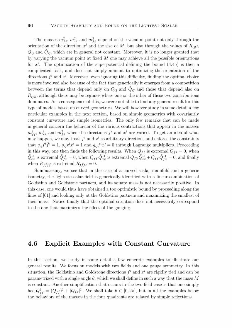
96 Vacuum Stability and Bound on the Lightest Scalar
The masses m2ff
, m2xx and m2
fx depend on the vacuum point not only through the
orientation of the direction xi and the size of M , but also through the values of Rikl,
Qi and Qi, which are in general not constant. Moreover, it is no longer granted that
by varying the vacuum point at fixed M one may achieve all the possible orientations
for xi. The optimization of the superpotential defining the bound (4.45) is then a
complicated task, and does not simply amount to optimizing the orientation of the
directions f i and xi. Moreover, even ignoring this difficulty, finding the optimal choice
is more involved also because of the fact that generically it emerges from a competition
between the terms that depend only on Qi and Qi and those that depend also on
Rikl, although there may be regimes where one or the other of these two contributions
dominates. As a consequence of this, we were not able to find any general result for this
type of models based on curved geometries. We will however study in some detail a few
particular examples in the next section, based on simple geometries with covariantly
constant curvature and simple isometries. The only few remarks that can be made
in general concern the behavior of the various contractions that appear in the masses
m2ff
, m2xx and m2
fx when the directions f i and xi are varied. To get an idea of what
may happen, we may treat f i and xi as arbitrary directions and enforce the constraints
that gifif = 1, gix
ix = 1 and gifix = 0 through Lagrange multipliers. Proceeding
in this way, one then finds the following results. When Qff is extremal Qfx = 0, when
Q–1xx is extremal Q–1
fx = 0, when Qff Q–1xx is extremal Qfx Q
–1xx+Qff Q
–1fx = 0, and finally
when Rfff f is extremal Rfffx = 0.
Summarizing, we see that in the case of a curved scalar manifold and a generic
isometry, the lightest scalar field is generically identified with a linear combination of
Goldstino and Goldstone partners, and its square mass is not necessarily positive. In
this case, one would thus have obtained a too optimistic bound by proceeding along the
lines of [61] and looking only at the Goldstino partners and maximizing the smallest of
their mass. Notice finally that the optimal situation does not necessarily correspond
to the one that maximizes the effect of the gauging.
4.6 Explicit Examples with Constant Curvature
In this section, we study in some detail a few concrete examples to illustrate our
general results. We focus on models with two fields and one gauge symmetry. In this
situation, the Goldstino and Goldstone directions f i and xi are rigidly tied and can be
parametrized with a single angle θ, which we shall define in such a way that the mass M
is constant. Another simplification that occurs in the two-field case is that one simply
has Q2ff
= (Qff )2 + |Qfx|2. We shall take θ ∈ [0, 2π], but in all the examples below
the behaviors of the masses in the four quadrants are related by simple reflections.
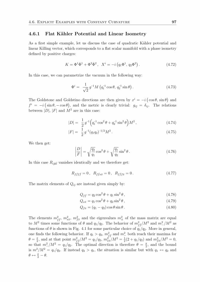
4.6. Explicit Examples with Constant Curvature 97
4.6.1 Flat Kahler Potential and Linear Isometry
As a first simple example, let us discuss the case of quadratic Kahler potential and
linear Killing vector, which corresponds to a flat scalar manifold with a phase isometry
defined by positive charges:
K = Φ1Φ1 + Φ2Φ2 , X i = −i(q1Φ1, q2Φ2
). (4.72)
In this case, we can parametrize the vacuum in the following way:
Φi =1√2g–1M
(q–1
1 cos θ, q–12 sin θ
). (4.73)
The Goldstone and Goldstino directions are then given by xi = −i(
cos θ, sin θ)
and
f i = −i(
sin θ,− cos θ), and the metric is clearly trivial: gi = δij. The relations
between |D|, |F | and M2 are in this case:
|D| = 1
2g–1(q–1
1 cos2 θ + q–12 sin2 θ
)M2 , (4.74)
|F | = 1
2g–1(q1q2)–1/2M2 . (4.75)
We then get: ∣∣∣∣DF∣∣∣∣ =
√q2
q1
cos2 θ +
√q1
q2
sin2 θ . (4.76)
In this case Rikl vanishes identically and we therefore get:
Rfff f = 0 , Rffxx = 0 , Rfffx = 0 . (4.77)
The matrix elements of Qi are instead given simply by:
Qff = q2 cos2 θ + q1 sin2 θ , (4.78)
Qxx = q1 cos2 θ + q2 sin2 θ , (4.79)
Qfx = (q1 − q2) cos θ sin θ . (4.80)
The elements m2ff
, m2xx, m
2fx and the eigenvalues m2
± of the mass matrix are equal
to M2 times some functions of θ and q1/q2. The behavior of m2ff/M2 and m2
−/M2 as
functions of θ is shown in Fig. 4.1 for some particular choice of q1/q2. More in general,
one finds the following behavior. If q1 > q2, m2ff
and m2− both reach their maxima for
θ = π2, and at that point m2
ff/M2 = q1/q2, m2
xx/M2 = 1
2(2 + q1/q2) and m2
fx/M2 = 0,
so that m2−/M
2 = q1/q2. The optimal direction is therefore θ = π2, and the bound
is m2/M2 = q1/q2. If instead q2 > q1, the situation is similar but with q1 ↔ q2 and
θ ↔ π2− θ.
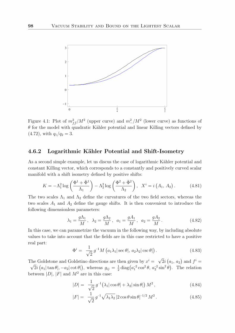
98 Vacuum Stability and Bound on the Lightest Scalar
0 !4
!2
"1
0
1
2
3
Figure 4.1: Plot of m2ff/M2 (upper curve) and m2
−/M2 (lower curve) as functions of
θ for the model with quadratic Kahler potential and linear Killing vectors defined by
(4.72), with q1/q2 = 3.
4.6.2 Logarithmic Kahler Potential and Shift-Isometry
As a second simple example, let us discus the case of logarithmic Kahler potential and
constant Killing vector, which corresponds to a constantly and positively curved scalar
manifold with a shift isometry defined by positive shifts:
K = −Λ21 log
(Φ1 + Φ1
Λ1
)− Λ2
2 log
(Φ2 + Φ2
Λ2
), X i = i
(A1, A2
). (4.81)
The two scales Λ1 and Λ2 define the curvatures of the two field sectors, whereas the
two scales A1 and A2 define the gauge shifts. It is then convenient to introduce the
following dimensionless parameters:
λ1 =gΛ1
M, λ2 =
gΛ2
M, a1 =
gA1
M, a2 =
gA2
M. (4.82)
In this case, we can parametrize the vacuum in the following way, by including absolute
values to take into account that the fields are in this case restricted to have a positive
real part:
Φi =1√2g–1M
(a1λ1| sec θ|, a2λ2| csc θ|
). (4.83)
The Goldstone and Goldstino directions are then given by xi =√
2i(a1, a2
)and f i =√
2i(a1| tan θ|,−a2| cot θ|
), whereas gi = 1
2diag
(a–2
1 cos2 θ, a–22 sin2 θ
). The relation
between |D|, |F | and M2 are in this case:
|D| = 1√2g–1(λ1| cos θ|+ λ2| sin θ|
)M2 , (4.84)
|F | = 1√2g–1√λ1λ2 |2 cos θ sin θ|–1/2M2 . (4.85)
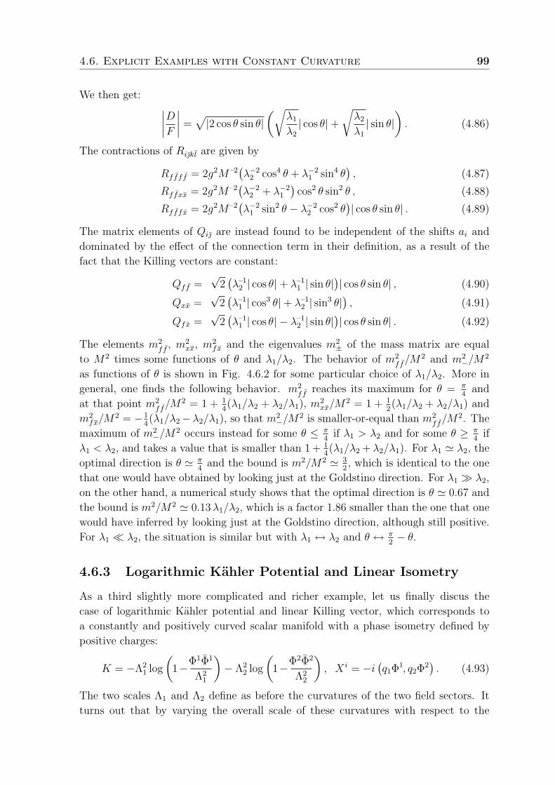
4.6. Explicit Examples with Constant Curvature 99
We then get: ∣∣∣∣DF∣∣∣∣ =
√|2 cos θ sin θ|
(√λ1
λ2
| cos θ|+√λ2
λ1
| sin θ|). (4.86)
The contractions of Rikl are given by
Rfff f = 2g2M–2(λ−2
2 cos4 θ + λ−21 sin4 θ
), (4.87)
Rffxx = 2g2M–2(λ−2
2 + λ−21
)cos2 θ sin2 θ , (4.88)
Rfffx = 2g2M–2(λ−2
1 sin2 θ − λ−22 cos2 θ
)| cos θ sin θ| . (4.89)
The matrix elements of Qi are instead found to be independent of the shifts ai and
dominated by the effect of the connection term in their definition, as a result of the
fact that the Killing vectors are constant:
Qff =√
2(λ–1
2 | cos θ|+ λ–11 | sin θ|
)| cos θ sin θ| , (4.90)
Qxx =√
2(λ–1
1 | cos3 θ|+ λ–12 | sin3 θ|
), (4.91)
Qfx =√
2(λ–1
1 | cos θ| − λ–12 | sin θ|
)| cos θ sin θ| . (4.92)
The elements m2ff
, m2xx, m
2fx and the eigenvalues m2
± of the mass matrix are equal
to M2 times some functions of θ and λ1/λ2. The behavior of m2ff/M2 and m2
−/M2
as functions of θ is shown in Fig. 4.6.2 for some particular choice of λ1/λ2. More in
general, one finds the following behavior. m2ff
reaches its maximum for θ = π4
and
at that point m2ff/M2 = 1 + 1
4(λ1/λ2 + λ2/λ1), m2
xx/M2 = 1 + 1
2(λ1/λ2 + λ2/λ1) and
m2fx/M
2 = −14(λ1/λ2−λ2/λ1), so that m2
−/M2 is smaller-or-equal than m2
ff/M2. The
maximum of m2−/M
2 occurs instead for some θ ≤ π4
if λ1 > λ2 and for some θ ≥ π4
if
λ1 < λ2, and takes a value that is smaller than 1 + 14(λ1/λ2 + λ2/λ1). For λ1 ' λ2, the
optimal direction is θ ' π4
and the bound is m2/M2 ' 32, which is identical to the one
that one would have obtained by looking just at the Goldstino direction. For λ1 λ2,
on the other hand, a numerical study shows that the optimal direction is θ ' 0.67 and
the bound is m2/M2 ' 0.13λ1/λ2, which is a factor 1.86 smaller than the one that one
would have inferred by looking just at the Goldstino direction, although still positive.
For λ1 λ2, the situation is similar but with λ1 ↔ λ2 and θ ↔ π2− θ.
4.6.3 Logarithmic Kahler Potential and Linear Isometry
As a third slightly more complicated and richer example, let us finally discus the
case of logarithmic Kahler potential and linear Killing vector, which corresponds to
a constantly and positively curved scalar manifold with a phase isometry defined by
positive charges:
K = −Λ21 log
(1−Φ1Φ1
Λ21
)− Λ2
2 log
(1−Φ2Φ2
Λ22
), X i = −i
(q1Φ1, q2Φ2
). (4.93)
The two scales Λ1 and Λ2 define as before the curvatures of the two field sectors. It
turns out that by varying the overall scale of these curvatures with respect to the
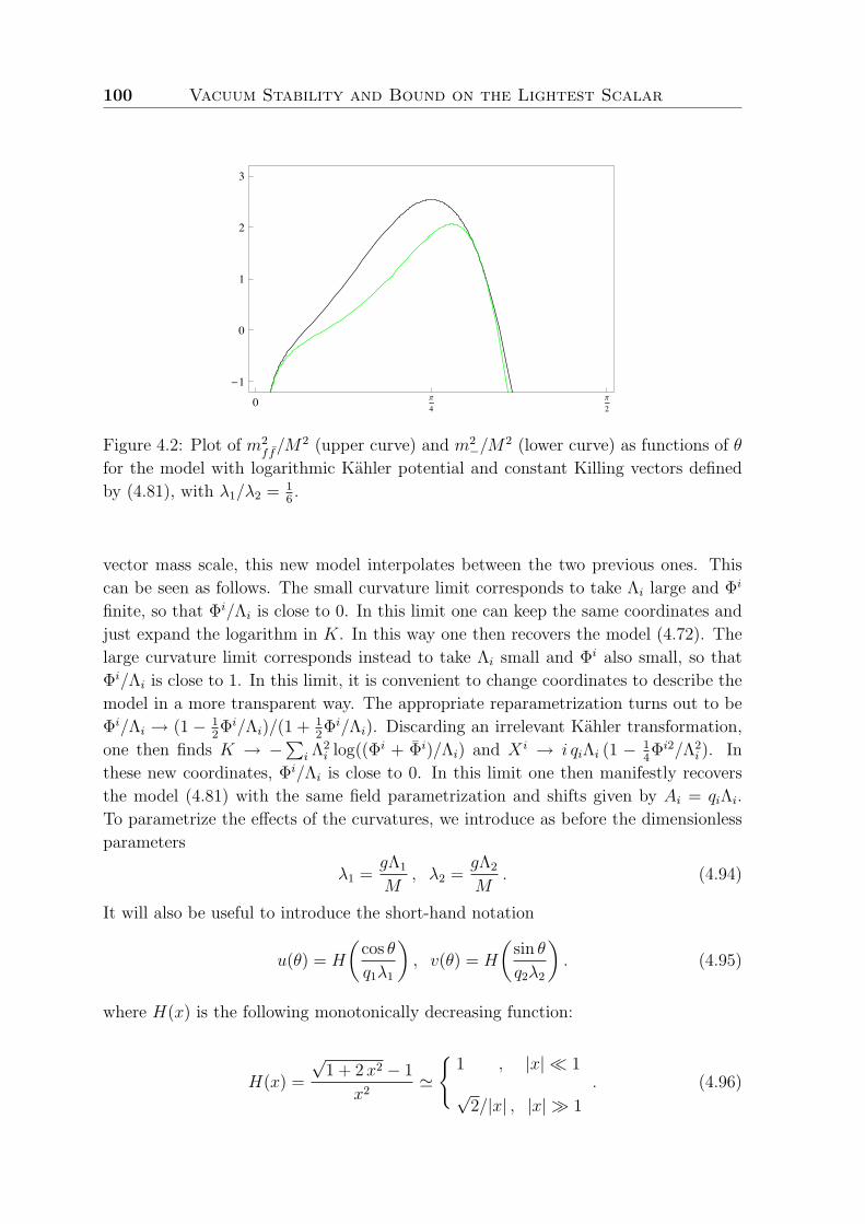
100 Vacuum Stability and Bound on the Lightest Scalar
0 !4
!2
"1
0
1
2
3
Figure 4.2: Plot of m2ff/M2 (upper curve) and m2
−/M2 (lower curve) as functions of θ
for the model with logarithmic Kahler potential and constant Killing vectors defined
by (4.81), with λ1/λ2 = 16.
vector mass scale, this new model interpolates between the two previous ones. This
can be seen as follows. The small curvature limit corresponds to take Λi large and Φi
finite, so that Φi/Λi is close to 0. In this limit one can keep the same coordinates and
just expand the logarithm in K. In this way one then recovers the model (4.72). The
large curvature limit corresponds instead to take Λi small and Φi also small, so that
Φi/Λi is close to 1. In this limit, it is convenient to change coordinates to describe the
model in a more transparent way. The appropriate reparametrization turns out to be
Φi/Λi → (1− 12Φi/Λi)/(1 + 1
2Φi/Λi). Discarding an irrelevant Kahler transformation,
one then finds K → −∑
i Λ2i log((Φi + Φi)/Λi) and X i → i qiΛi (1 − 1
4Φi2/Λ2
i ). In
these new coordinates, Φi/Λi is close to 0. In this limit one then manifestly recovers
the model (4.81) with the same field parametrization and shifts given by Ai = qiΛi.
To parametrize the effects of the curvatures, we introduce as before the dimensionless
parameters
λ1 =gΛ1
M, λ2 =
gΛ2
M. (4.94)
It will also be useful to introduce the short-hand notation
u(θ) = H
(cos θ
q1λ1
), v(θ) = H
(sin θ
q2λ2
). (4.95)
where H(x) is the following monotonically decreasing function:
H(x) =
√1 + 2 x2 − 1
x2'
1 , |x| 1
√2/|x| , |x| 1
. (4.96)
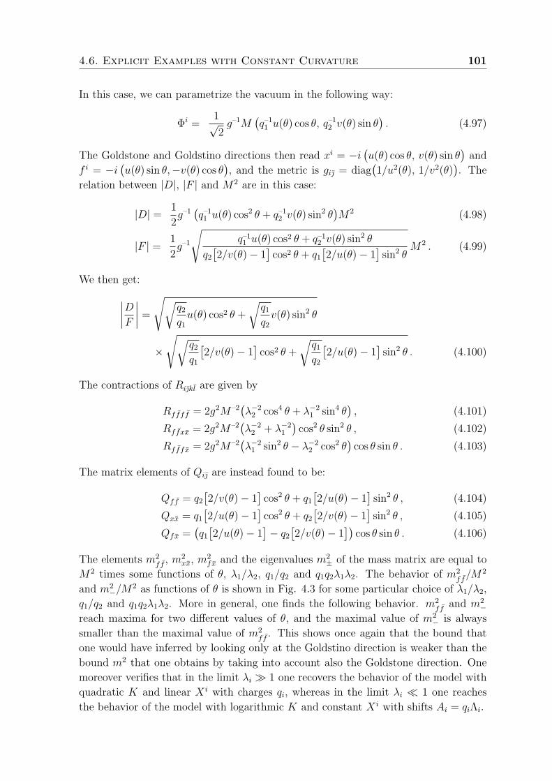
4.6. Explicit Examples with Constant Curvature 101
In this case, we can parametrize the vacuum in the following way:
Φi =1√2g–1M
(q–1
1 u(θ) cos θ, q–12 v(θ) sin θ
). (4.97)
The Goldstone and Goldstino directions then read xi = −i(u(θ) cos θ, v(θ) sin θ
)and
f i = −i(u(θ) sin θ,−v(θ) cos θ
), and the metric is gi = diag
(1/u2(θ), 1/v2(θ)
). The
relation between |D|, |F | and M2 are in this case:
|D| = 1
2g–1(q–1
1 u(θ) cos2 θ + q–12 v(θ) sin2 θ
)M2 (4.98)
|F | = 1
2g–1
√q–1
1 u(θ) cos2 θ + q–12 v(θ) sin2 θ
q2
[2/v(θ)− 1
]cos2 θ + q1
[2/u(θ)− 1
]sin2 θ
M2 . (4.99)
We then get:∣∣∣∣DF∣∣∣∣ =
√√q2
q1
u(θ) cos2 θ +
√q1
q2
v(θ) sin2 θ
×
√√q2
q1
[2/v(θ)− 1
]cos2 θ +
√q1
q2
[2/u(θ)− 1
]sin2 θ . (4.100)
The contractions of Rikl are given by
Rfff f = 2g2M–2(λ−2
2 cos4 θ + λ−21 sin4 θ
), (4.101)
Rffxx = 2g2M–2(λ−2
2 + λ−21
)cos2 θ sin2 θ , (4.102)
Rfffx = 2g2M–2(λ−2
1 sin2 θ − λ−22 cos2 θ
)cos θ sin θ . (4.103)
The matrix elements of Qi are instead found to be:
Qff = q2
[2/v(θ)− 1
]cos2 θ + q1
[2/u(θ)− 1
]sin2 θ , (4.104)
Qxx = q1
[2/u(θ)− 1
]cos2 θ + q2
[2/v(θ)− 1
]sin2 θ , (4.105)
Qfx =(q1
[2/u(θ)− 1
]− q2
[2/v(θ)− 1
])cos θ sin θ . (4.106)
The elements m2ff
, m2xx, m
2fx and the eigenvalues m2
± of the mass matrix are equal to
M2 times some functions of θ, λ1/λ2, q1/q2 and q1q2λ1λ2. The behavior of m2ff/M2
and m2−/M
2 as functions of θ is shown in Fig. 4.3 for some particular choice of λ1/λ2,
q1/q2 and q1q2λ1λ2. More in general, one finds the following behavior. m2ff
and m2−
reach maxima for two different values of θ, and the maximal value of m2− is always
smaller than the maximal value of m2ff
. This shows once again that the bound that
one would have inferred by looking only at the Goldstino direction is weaker than the
bound m2 that one obtains by taking into account also the Goldstone direction. One
moreover verifies that in the limit λi 1 one recovers the behavior of the model with
quadratic K and linear X i with charges qi, whereas in the limit λi 1 one reaches
the behavior of the model with logarithmic K and constant X i with shifts Ai = qiΛi.
102 Vacuum Stability and Bound on the Lightest Scalar
0 !4
!2
"1
0
1
2
3
Figure 4.3: Plot of m2ff/M2 (upper curve) and m2
−/M2 (lower curve) as functions of θ
for the model with logarithmic Kahler potential and linear Killing vectors defined by
(4.93), with λ1/λ2 = 16, q1/q2 = 3 and q1q2λ1λ2 = 1.
4.7 Summary
In this chapter, we have shown that it is possible to derive an absolute upper bound
on the mass of the lightest scalar field of a theory with spontaneously broken su-
persymmetry and local gauge symmetries. This can be obtained by focusing on the
subset of scalar fields corresponding to the partners of the Goldstino fermion and the
gauge vector bosons, for which the mass is constrained by symmetry arguments. The
resulting bound has the property that it can be saturated by adjusting the superpo-
tential. Requiring it to be positive is therefore a necessary and sufficient condition on
the remaining functions specifying the kinetic terms for the existence of a metastable
supersymmetry-breaking vacuum. We have shown that by including also the Goldstone
partners one finds in general a stronger bound than by considering just the Goldstino
partners, and we have illustrated this fact through several explicit examples.
The results we presented in this chapter have interesting implications on the condi-
tions for the existence of metastable supersymmetry breaking vacua in generic super-
symmetric theories with local gauge symmetries. Indeed, the region of parameter space
where tachyons can be avoided is reduced when one considers not only the Goldstino
partners but also the Goldstone partners, since there are points where the former have
positive square mass while the latter or linear combinations of the two have negative
square mass. We believe that there may in fact exist models where the upper bound
derived from just the Goldstino partners is positive whereas the upper bound derived
by including also the Goldstone partners is negative. In such a situation, one would
then find an obstruction against the existence of metastable supersymmetry-breaking
vacua that comes from the Goldstone partners rather than from the Goldstino partners.
4.7. Summary 103
In the light of this possibility, it would be interesting to apply the result that we have
derived to reexamine the conditions for the existence of metastable supersymmetry-
breaking vacua in theories where the gauging plays a crucial role. One class of models
where this could perhaps uncover new instabilities is that of theories with extended su-
persymmetry, and more specifically those where the Goldstino partners do not seem to
lead necessarily to tachyons. This is for instance the case of N = 2 theories with non-
Abelian vector multiplets and/or charged hyper multiplets (see [128] for an extended
discussion on this topic).
To conclude, we would like to comment on the generalization of our result to the
case of supergravity theories. The only technical difficulty to extend our analysis to
that case is the fact that the Goldstino direction f i and the Goldstone directions xiaare no longer orthogonal, as a consequence of the additional gravitational term in
the definition of the auxiliary fields. More precisely, one gets gifixa = ig–1m3/2Da.
As a consequence, the set of vectors f i and xia can no longer be chosen to form an
orthonormal set, although it still represents a complete set of dangerous directions. The
restriction of the mass matrix to this subspace is then no longer given just by eq. (4.25)
but by a more complex expression. As a result, the analysis becomes technically more
complicated. But for the rest one can apply the same strategy we developed in this
chapter for theories with rigid supersymmetry.

104
Chapter 5
Effects of Heavy Multiplets on
Vacuum Stability
In this chapter we are going to combine the main results of the previous two chapters
to study the effects induced by heavy supermultiplets on the masses of light scalar
fields and in particular on the metastability conditions; this is done in the limit in
which the heavy mass scale is much larger than the supersymmetry breaking scale and
heavy multiplets can be integrate out supersymmetrically by following the procedure
described in Chapter 3. We restrict to the case in which all the vector multiplets
have large supersymmetric masses and the low-energy supersymmetric effective theory
contains only light chiral multiplets. As we have seen at the end of Section 4.2, in this
situation the Goldstino is the only dangerous direction in the scalar field space whereas
the directions associated to Killing vectors are automatically safe.
We will show that the square-masses of light scalar fields can get two different types
of significant corrections when a heavy multiplet is integrated out. The first is an indi-
rect level-repulsion effect, which may arise from heavy chiral multiplets and is always
negative. The second is a direct coupling contribution, which may arise from heavy
vector multiplets and can have any sign. We then apply these results to the sGoldstino
mass and study the implications for the vacuum metastability condition. We find that
the correction from heavy chiral multiplets is always negative and tends to compromise
vacuum metastability, whereas the contribution from heavy vector multiplets is always
positive and tends on the contrary to reinforce it. These two effects are controlled re-
spectively by Yukawa couplings and gauge charges, which mix one heavy and two light
fields respectively in the superpotential and the Kahler potential. Finally we will also
comment on similar effects induced in soft scalar masses when the heavy multiplets
couple both to the visible and the hidden sector. This chapter is based on our paper
[3].
105
106 Effects of Heavy Multiplets on Vacuum Stability
5.1 General Considerations
In the following we are interested in studying the low-energy dynamics and in partic-
ular the question of vacuum metastability within the supersymmetric effective theory
obtained by integrating out heavy fields in a manifestly supersymmetric way. In Chap-
ter 3 we have shown that at leading order in the low-energy expansion in the number
of derivatives, fermions and auxiliary fields, the basic recipe is that chiral and vector
superfields can be integrated out by using approximate equations of motion correspond-
ing to imposing stationarity of W and K respectively. In the forthcoming sections we
will make more explicit the computation of the scalar masses in the low energy effec-
tive theory in the case in which only chiral multiplets are light; as anticipated, this
analysis may play a relevant role in the study of the moduli sector of string models
where supersymmetry is supposed to be spontaneously broken (see Section 2.3).
More specifically, we ask the practical question of what is the effect of heavy modes
on the light masses, and in particular whether the induced corrections tend to improve
or to worsen the situation concerning metastability of the vacuum. It would be very
valuable to have some criterion to distinguish situations where the effect of heavy
modes on the scalar square-masses are negative, and must therefore necessarily be
computed to be able to assess vacuum stability, from situations where this effect is
positive and can thus be safely ignored to check vacuum metastability. To derive
such a criterion, we shall study in some detail the structure and the sign of the effect
induced by heavy modes on the sGoldstino mass, which captures the crucial condition
for achieving metastability. Most of the details are developed for simplicity in the
rigid case; however, as we explained in Chapter 3 gravity does not introduce new
complications and a similar analysis can be performed in the supergravity case. We
comment on these aspects at the end of the chapter.
In order to illustrate the basic point that we want to make, let us consider a generic
theory involving both light and heavy modes, indicated as φi and φα respectively, that
interact among each other. For simplicity, we shall think of these as real scalar fields
in a non-supersymmetric theory, but the results are clearly more general. In such
a situation, one may define a low-energy effective theory for the light modes φi by
integrating out the heavy modes φα. As we already discussed, at lowest order in the
low-energy expansion, this can be done by requiring stationarity of the potential energy
V with respect to the heavy modes and solving the equation Vα = 0. This determines
φα = φα0 (φi). By differentiating the stationarity equation with respect to the light
fields, one also deduces that ∂iφα0 = −V αβ
inv Vβi, where V αβinv denotes the inverse of Vαβ as
a matrix.1
1We use ( )inv instead of ( )−1 to indicate inverse matrices in order to clearly distinguish betweentwo different kinds of inverse matrices which appear in the computations. More precisely, consider ageneral square matrix X; as a general rule we adopt the convention that the subscript “inv” definesthe inverse of an arbitrary invertible sub-block of X, whereas the symbol “-1” is used to represent theinverse of the whole matrix X. For example, Xαβ
inv represents the inverse of the sub-block Xαβ whereasX−1αβ represents the (αβ) components of the inverse matrix X−1. It is then obvious that in general
5.2. Effect of Heavy Chiral Multiplets 107
The effective Lagrangian for the low-energy theory is then obtained, as usual, by
substituting back this solution into the original Lagrangian. For the wave-function
factor and the potential, one easily obtains geffij (φi) = (gij + ∂iφ
α0 gαj + ∂jφ
β0giβ +
∂iφα0∂jφ
β0gαβ)(φi, φα0 ) and V eff(φi) = V (φi, φα0 (φi)). The light masses may finally be
derived by computing derivatives of V eff . Using the chain rule, these can be related
to derivatives of V . One finds V effi = Vi and V eff
ij = Vij − ViαV αβinv Vβj, so that the light
masses m2effij = V eff
ij are given by the following expression in terms of the light, heavy
and mixing blocks m2ij = Vij, M
2αβ = Vαβ and µ2
iα = Viα of the full mass matrix:
m2effij = m2
ij − µ2iαM
−2αβµ2βj . (5.1)
This expression is easily seen to coincide with the mass matrix of light states obtained
by diagonalizing the full mass matrix of the microscopic theory at leading order in an
expansion in powers of the inverse heavy mass matrix. The formula (5.1) moreover
shows that integrating out the heavy modes generically gives two types of effects on
the masses of the light modes. The first is a direct effect hidden in the first term on
the right hand side and is due to the fact that the light block of the mass matrix m2ij
gets influenced by the coupling to the heavy modes. It has a sign that depends on
the form of the couplings between light and heavy modes. The second is an indirect
effect described by the second term on the right-hand side and is due to the fact that
the presence of an off-diagonal block in the mass matrix mixing light and heavy fields
makes the true light mass matrix differ from the original light block. It has a sign that
is manifestly always negative. In parallel with what happens to a quantum mechanical
system with two separated sets of low and high energy levels, we see that there is a
direct effect correcting significantly the light energy levels and negligibly the heavy
ones, which is due to diagonal interactions and can have any sign, and an indirect
level-repulsion effect that further splits apart the two sets of levels, which is due to
off-diagonal interactions and has a definite sign.
5.2 Effect of Heavy Chiral Multiplets
Let us now consider a situation where the chiral multiplets ΦI split into a set of light
multiplets Φi parametrizing the low-energy theory and a set of heavy multiplets Φα 2
with a large supersymmetric mass Wαβ to be integrated out. For later convenience we
recall the expressions of the scalar masses discussed in Section 1.3.1:
m20IJ = ∇IWK∇JW
K −RIJKL FKF L , (5.2)
m20IJ = −∇I∇JWK F
K . (5.3)
situations Xαβinv and X−1αβ do not coincide.
2Notice that here we come back to the notation of Chapter 3 in which capital indices indicatecollectively light and heavy fields.
108 Effects of Heavy Multiplets on Vacuum Stability
In order to distinguish light from heavy multiplets in a sensible way, we must assume
that the supersymmetric mass mixing Wiα between them is not too large. We denote
the heavy, light and mixing blocks of the whole supersymmetric mass matrix M1/2 in
the following way:
M1/2 =
M µ
µ† m
, (5.4)
where
Mαβ = Wαβ , µαi = Wαi , mij = Wij . (5.5)
The most relevant interactions for our purposes will be the cubic terms in W , namely
the Yukawa couplings (3.27)
λαij = Wαij , λαβj = Wαβj , λαβγ = Wαβγ . (5.6)
At leading order in the low-energy expansion in number of derivatives, fermions
and auxiliary fields, the low-energy effective theory can be obtained in component
fields by imposing stationarity of V with respect to each heavy field and substituting
back the solution into the original Lagrangian. Equivalently, this effective theory can
be derived directly in superfields, by demanding the stationarity of W with respect to
each heavy chiral multiplet. For convenience, we shall assume without loss of generality
normal coordinates in the microscopic theory around the point under consideration.
This substantially simplifies the computations, although the effective theory does not
automatically inherit normal coordinates, due to the corrections induced to the Kahler
metric.
The holomorphic coordinate transformations to go in normal coordinates is defined
by asking that the Kahler connection Γ is locally vanishing at an arbitrary point of the
scalar manifold. We get (see for example [129]):
ΦI′ = ΛI′
I
(ΦI +
1
2ΓIJK |ΦJΦK +
1
6gIL∂PΓLJK |ΦJΦKΦP + · · ·
), (5.7)
where ΛI′I is defined in such a way that:
KI′J ′| = δI′J ′ = Λ II′Λ
J
J ′KIJ | . (5.8)
In the new coordinate system, the Kaheler potential can locally be approximated as:
K(Φ, Φ) = K|+ F (Φ) + F (Φ) + δIJ ΦIΦJ +1
4RIJKL|ΦIΦJΦKΦL +O(Φ5) , (5.9)
where F is an irrelevant holomorphic function. The Kahler metric is then:
gIJ(Φ, Φ) = δIJ +RIJKL|ΦKΦL +O(Φ3) . (5.10)
5.2. Effect of Heavy Chiral Multiplets 109
We stopped at fourth order in the expansion of K since higher terms do not contribute
in the computation of sGoldstinos mass.
The corrections due to the supersymmetric mass mixing between heavy and light
multiplets are encoded in the following small dimensionless matrix:
εαi = −M−1αβµβi . (5.11)
It should be emphasized that it is always possible to perform a holomorphic field
redefinition in such a way to diagonalize the supersymmetric mass matrix WIJ at a
given point in field space, thereby setting εαi to zero. This means that all the effects
depending on εαi only serve to compensate a choice of light and heavy fields that does
not exactly diagonalize the supersymmetric part of the mass matrix, and therefore
do not represent genuine non-trivial corrections. Moreover, since εαi must be small,
these effects are anyhow quantitatively irrelevant. We may then set εαi = 0 by suitably
choosing the fields. We shall however keep εαi 6= 0 during the computations to verify
more explicitly the above claims and set εαi = 0 only at the very end. We can anticipate
that all the tensorial quantities characterizing the light fields will receive additional
contributions coming from heavy indices converted to light indices through the matrix
εαi . This leads us to introduce already at this stage the following deformed tensors:
gεi = gi + εαi gα + εβ giβ + εαi εβ gαβ , (5.12)
λεαij = λαij + εβi λαβj + εγjλαiγ + εβi εγjλαβγ , (5.13)
Rεikl = Rikl + εαi Rαkl + εβRiβkl + εγkRiγl + εδlRikδ + εαi ε
βRαβkl
+ εαi εγkRαγl + εαi ε
δlRαkδ + εβ ε
γkRiβγl + εβ ε
δlRiβkδ + εγk ε
δlRiγδ
+ εβ εγk εδlRiβγδ + εαi ε
γk εδlRαγδ + εαi ε
β εδlRαβkδ + εαi ε
β εγkRαβγl
+ εαi εβ εγk εδlRαβγδ . (5.14)
Finally, we shall define the following quantity for later use, which characterizes the
heavy block WαI gIJ WJ β of the square of the supersymmetric mass matrix:
|M ε|2αβ = Mαγ
(gγδ + εγi g
iδ + εδgγ + εγi ε
δgi)Mδβ . (5.15)
In the following, we shall compute within the component approach the average
sGoldstino mass in the low-energy effective theory, defined at a stationary point as 3
m2effϕ =
m2eff0i F
ieffF eff
F keffF effk
. (5.16)
We shall then reproduce the same result within the superfield approach by first com-
puting the Riemann tensor Reffikl
of the effective theory at a generic point and then
3For convenience in this chapter we indicate the mass in the Goldstino direction by m2ϕ, avoiding
the heavier notation m2ff
which would be confusing when generalized to the effective theory. For thesame reason we will also avoid the symbol Rffff introduced in the previous chapter to denote thecontraction of the Riemann tensor with the Goldstino direction.
110 Effects of Heavy Multiplets on Vacuum Stability
applying the standard expression for the sGoldstino mass at a stationary point (4.28),
correctly reinterpreted in the new notation and applied to the effective theory where
no vector multiplets are present. The relevant formula is:
m2effϕ = ReffF ieffF eff
i , (5.17)
where we defined the effective sectional curvature 4
Reff = −ReffiklF ieffF effF keffF leff
(FmeffF effm )2
. (5.18)
5.2.1 Component Approach
Consider first the component approach. For simplicity we shall focus on the bosonic
fields and discard fermions, since we are interested in computing effective scalar masses;
in the low-energy expansion the values of the heavy scalar fields are defined by
φα = φα0 (φi, φı) solution of Vα(φi, φı, φα0 , φα0 ) = 0 . (5.19)
At leading order in the number of auxiliary fields, this stationarity condition implies
that WαIWI = 0 and gives the following values for the heavy auxiliary fields:
Fα = εαi Fi . (5.20)
The effective theory for the light fields is then obtained by substituting these expressions
for φα and Fα into the original Lagrangian.
To derive the effective theory, we will need to compute the derivatives of the heavy
fields φα0 and φα0 with respect to the light fields φi. These can be deduced, as in the
non-supersymmetric case, by differentiating the stationarity conditions Vα = 0 with
respect to the light fields. One finds:
∂φα
∂φi= −M−2αβ
0 µ20βi −M
−2αβ0 µ2
0βi , (5.21)
∂φα
∂φi= −M−2αβ
0 µ20βi −M
−2αβ0 µ2
0βi . (5.22)
where we defined the heavy and off-diagonal blocks of the complete scalar mass matrix
M20 of the microscopic theory:
M20 =
M20 µ2
0
µ† 20 m2
0
, (5.23)
4Notice the minus sign introduced to match the usual definition of sectional curvature for realmanifolds. See App. B of [130].
5.2. Effect of Heavy Chiral Multiplets 111
where
M20 =
Vαβ Vαβ
Vαβ Vαβ
, µ20 =
Vα Vαj
Vα Vαj
, m20 =
Vi Vij
Vı Vıj
, (5.24)
Notice that µ0 and M0 differ from µ and M , since the former refer to the full mass
matrix (5.2)-(5.3) whereas the latter parametrize only its supersymmetric part, namely
WIJ . More precisely:
(M20 )αβ = Vαβ , (µ2
0)α = Vα , (m20)i = Vi , (5.25)
coincide with M2, µ2 and m2 in (5.5) only in the supersymmetric limit. At quadratic
order in the auxiliary fields one finds:
M−2αβ0 = V αβ
inv + V αγinv Vγδ V
δσinvVστ V
τβinv , (5.26)
M−2αβ0 = −V αγ
inv Vγδ Vδβ
inv . (5.27)
It is convenient for the forthcoming analysis to roughly estimate the leading powers of
auxiliary fields F in each term of previous expressions. We have that V αβinv ∼ aF 0 +
b F 2 +O(F 3) whereas Vαβ ∼ c F and this implies, at quadratic order in F , that M−2αβ0
contains only terms which are quadratic or constant in F whereas M−2αβ0 contains only
linear terms.
The effective Kahler metric of the light fields can be determined by looking at the
scalar kinetic terms and substituting the values of the heavy scalar fields. One may in
this case work at leading order in the auxiliary fields, since these terms already involve
two derivatives. Focusing also on the leading order in the light masses and the heavy-
light mass mixing, the relations (5.21) and (5.22) then simplify to ∂iφα = εαi + O(F )
and ∂iφα = O(F ). Using these expressions, which actually turn out to be correct
even at order ε2, one finds that the kinetic term can be rewritten in the standard
supersymmetric form with an effective Kahler metric given by
geffi = gεi . (5.28)
The effective mass matrix of the light scalar fields can on the other hand be deter-
mined by using the supersymmetric generalization of the expression (5.1), which can
be derived by using the same logic. More precisely the effective masses are obtained by
taking holomorphic and anti-holomorphic derivatives of V effi = Vi+Vα
∂φα0∂φi
+Vα∂φα0∂φi
= Vi.
One then finds:
m2eff0i = m2
0i − µ20iαM
−2αβ0 µ2
0β − µ20iαM
−2αβ0 µ2
0β
− µ20iαM
−2αβ0 µ2
0β − µ20iαM
−2αβµ20β , (5.29)
m2eff0ij = m2
0ij − µ20iαM
−2αβ0 µ2
0βj − µ20iαM
−2αβ0 µ2
0βj
− µ20iαM
−2αβ0 µ2
0βj − µ20iαM
−2αβ0 µ2
0βj . (5.30)
112 Effects of Heavy Multiplets on Vacuum Stability
As in the general non-supersymmetric case, the result corresponds to a perturbative
diagonalization of the full scalar mass matrixM20, at leading order in the inverse mass
matrix of the heavy scalars M−20 :
m2eff0 = m2
0 − µ† 20 M−2
0 µ20 . (5.31)
Let us now focus on the Hermitian block m2eff0i . Using eqs. (5.26) and (5.27) in the
formula (5.29), and restricting to terms that are at most quadratic in the auxiliary
fields as demanded by supersymmetry at the two-derivative level, we see that there are
three kinds of effects coming from the four correction terms. The first type involves
second derivatives of W and no auxiliary fields, and comes only from the first correction
term. The second type involves the Riemann tensor and two auxiliary fields, and comes
again only from the first correction term. The third type involves third derivatives of
W and two auxiliary fields, and comes from all four correction terms. All together,
these three effects give a negative level-repulsion correction with respect to m20i.
Let us now compute more specifically the average sGoldstino mass m2effϕ defined by
eq. (5.16) at a stationary point of the effective theory and compare it to its analogue
m2ϕ = m2
0ifif in the microscopic theory. Recall that we are using normal coordinates,
so that gi = δi and geffi = δi + εαi ε
α . The first thing we need to make more explicit
are the effective auxiliary fields. To do so we start by deriving W eff by substituting the
solution (5.19) into in W . Taking a derivative we then find that W effi = Wi + εαiWα.
But using the stationarity condition WαIWI = 0 of the heavy scalars we see that
Wα = εαıWi, so that W effi = (δi + εαi ε
α )Wj = geff
i Wj. The auxiliary fields in the
effective theory thus coincide with the light components of the auxiliary fields in the
microscopic theory: F ieff = −geffiW eff = −Wı = F i. Recalling (5.20) one also finds
that geffi F
ieffF eff = F IF I . In summary, we get:
F ieff = F i , F ieffF effi = F IFI . (5.32)
To proceed, we also need to compute more explicitly the mass-matrix blocks (5.26) and
(5.27) entering in the expression (5.29) for the effective mass matrix m2eff0i . In normal
coordinates, these quantities depend on |M ε|2αβ
= Mαγ
(gγδ + εγi ε
δı
)Mδβ (see expression
(5.15)), and at quadratic order in the auxiliary fields one finds that
Vαβ = |M ε|2αβ −RαβKLFKF L , (5.33)
Vαβ = −λαβKFK , (5.34)
V αβinv = |M ε|−2αβ + |M ε|−2αδ|M ε|−2βγRγδKLF
KF L . (5.35)
We are now in position to evaluate the average sGoldstino mass in the effective the-
ory by computing the four correction terms in eq. (5.29). As explained after eqs. (5.29)
and (5.30), these give rise to three types of effects. But when looking along the sGold-
stino direction, some simplifications occur, due to the fact that only supersymmetry-
breaking effects matter. The first type of effect cancels the corresponding leading part
5.2. Effect of Heavy Chiral Multiplets 113
of m20i. The second type of effect combines with the corresponding subleading term in
m20i to reconstruct the average sGoldstino mass of the microscopic theory. The third
type of effect gives instead a genuine correction. The precise evaluation of these effects
can be simplified by noticing that at a stationary point WIJWJ = 0, which implies that
at leading order in the auxiliary fields VαıWi = −VαβWβ. After a straightforward com-
putation one finds that m2effϕ = −
(RIJKL + λαIK |M ε|−2αβλβJL
)F IF JFKF L/FM FM .
Recalling then that Fα = εαi Fieff and F IFI = F ieffF eff
i , one may finally rewrite the
above result as
m2effϕ =
(Rε − λεα|M ε|−2αβλεβ
)F ieffF eff
i , (5.36)
with
Rε = −RεiklF ieffF effF keffF leff
(FmeffF effm )2
, (5.37)
λεα =λεαijF
ieffF jeff
F keffF effk
. (5.38)
The first term in the result (5.36) corresponds to m2ϕ, whereas the second term describes
a negative level-repulsion effect controlled by the Yukawa couplings λαij mixing one
heavy and two light fields. As anticipated, the dependence on ε amounts to a transfor-
mation of all the tensorial quantities accounting for the need to disentangle light from
heavy eigenmodes of the supersymmetric mass matrix, and can thus be dropped by
setting ε to zero.
5.2.2 Superfield Approach
The above results can also be derived by integrating out the heavy fields directly at
the superfield level, and then computing the sGoldstino mass in the resulting effective
theory by applying eqs. (5.17) and (5.18). To do this, one derives the effective Kahler
potential and superpotential by solving the following approximate superfield equations
of motion:
Φα = Φα(Φi) solution of Wα(Φi,Φα) = 0 . (5.39)
As discussed in Chapter 3, the bosonic components of this superfield equations of
motion coincide, at leading order in the number of fermions and auxiliary fields, with
the equations of motion (5.19)–(5.20) that we have used in the component approach.
To proceed, we will need to compute the first and second derivatives of the heavy
scalar fields with respect to the light scalar fields. These can be derived by differenti-
ating eq. (5.39), and one finds the following results:
∂φα
∂φi= εαi ,
∂2φα
∂φi∂φj= −M−1αβλεβij . (5.40)
The effective geometry can be derived by taking derivatives with respect to the light
fields of the effective Kahler potential Keff , where the heavy fields have been substituted
114 Effects of Heavy Multiplets on Vacuum Stability
by the solution (5.39) in terms of light fields. We focus again on a given point in the light
field space, around which we choose normal coordinates, but this point no longer needs
to be a stationary point. Then, using the chain rule and eqs. (5.40), one easily computes
Keffi = δi+ε
αi εα , Keff
ıjk = −M−1αβ εαı λεβjk and Keff
ikl= Rε
ikl+λεαik|M |−2αβλε
βl. This finally
implies that the effective metric is given by geffi = gεi, the effective Christoffel symbol
by Γeffıjk = −M−1αβ εαı λ
εβjk and finally the effective Riemann tensor by the following
expression:
Reffikl = Rε
ikl + λεαik|M ε|−2αβλεβ l . (5.41)
Plugging this expression into eqs. (5.17) and (5.18), we then reproduce the form of the
result (5.36).5
5.3 Effect of Heavy Vector Multiplets
Let us now suppose that all the vector multiplets have a large supersymmetric mass,
much larger than the splittings induced by supersymmetry breaking. We may then
integrate out in a supersymmetric way the modes associated with these heavy vector
multiplets, paying attention to the fact that in order to become massive they absorb
the modes of some chiral multiplets.
For later convenience we recall the expressions of the scalar masses discussed in
Section 1.3.2:
m20IJ = ∇IWK∇JW
K −RIJKL FKF L + habXaIXbJ + habhacIhbdJ D
bDc
+(i∇IXaJ − ihbchabIXcJ + ihbchabJXcI
)Da , (5.42)
m20IJ = −∇I∇JWK F
K − habXaIXbJ −1
2
(∇IhabJ − 2hcdhacIhbdJ
)DaDb
+ 2i hbchab(IXcJ)Da , (5.43)
and the relation between F and D auxiliary fields valid at the vacuum (1.53):
i∇IXaJ FIF J − gIJXI
(aXJb) D
b +1
2f dab θdcD
bDc = 0 . (5.44)
The relevant scales in this case are the supersymmetric mass matrix 2gIJXI(aX
Jb) =
12Kab of the heavy vector multiplets and the quantity iXaI = 1
2KaI controlling the
supersymmetric mixing between vector multiplets and chiral multiplets:
M2ab =
1
2Kab , νaI =
1
2KaI . (5.45)
5Note that the results derived in this subsection are evaluated at values of the heavy scalar fieldssolving Wα = 0, whereas the results of previous subsection were evaluated at values of the heavy scalarfields solving Vα = 0. However it turns out that the difference between these two values is subleadingin the counting of auxiliary fields and can therefore be discarded.
5.3. Effect of Heavy Vector Multiplets 115
The couplings that are expected to be relevant are instead given by the cubic couplings
in K, namely the generalized charges
QaIJ = −1
2KaIJ , QabI = −1
2KabI , Qabc = −1
2Kabc . (5.46)
At leading order in the expansion in number of derivatives, fermions and auxil-
iary fields, the low-energy effective theory for the light chiral multiplets can again be
obtained in two different but equivalent ways. One may proceed in components and
integrate out the heavy modes associated to the vector multiplets and the chiral multi-
plets that they absorb, by requiring stationarity of V with respect to them. One may
however also proceed in superfields and integrate out the heavy vector superfields by
requiring stationarity of K with respect to them. For convenience, we shall as before
assume without loss of generality normal coordinates in the microscopic theory around
the point under consideration.
In analogy with what happens in the case of only chiral multiplets, we expect that
the corrections due to the supersymmetric mixing between heavy and light multiplets
should be encoded in following parameter of dimension one:
δaI = −M−2abνbI . (5.47)
In this case, such a parameter cannot be set to zero by a simple holomorphic field
redefinition, because it corresponds to the non-holomorphic mixing between the heavy
gauge fields and the corresponding real would-be Goldstone modes. However, it can be
set to zero by making a suitable choice of gauge. With any different choice of gauge, δaIwould be non-zero and the terms depending on it in the effective theory would take into
account the mixing between light and heavy fields. By doing the computation in such
a gauge one would presumably end up getting deformed versions of all the tensorial
quantities for light fields, involving additional contributions where heavy indices are
converted to light indices by δaI . We shall however refrain from keeping a general δaI 6= 0
and set δaI = 0 from the beginning by choosing the unitary gauge.
To perform the splitting between light and heavy fields and the gauge fixing more
precisely, we may start by splitting the chiral multiplets ΦI into those that are or-
thogonal and those that are parallel to the Killing vectors XIa evaluated at the point
under consideration. This decomposition can be done more explicitly with the help of
the parallel projector P IJ = 2XI
aM−2abXbJ . We shall denote these two sets of fields
respectively with Φi and Φa. The orthogonal components Φi define the light chiral
multiplets of the low-energy effective theory. The parallel components Φa are instead
either heavy or eliminable through the gauge fixing.
In the following, we shall follow the same logic as in the previous section and first
compute within the component approach the average sGoldstino mass in the low-energy
effective theory, defined at a stationary point as
m2effϕ =
m2eff0i F
ieffF eff
F keffF effk
. (5.48)
116 Effects of Heavy Multiplets on Vacuum Stability
As we discussed in the previous chapter, in the limit in which the vector masses are
much larger than the supersymmetry breaking scale, the danger associated to the
Killing directions disappear, and the Goldstino direction is the only relevant direction
we should consider to discuss metastability.
We will finally reproduce the same result within the superfield approach by first
computing the Riemann tensor of the effective theory at a generic point and then
plugging it in the expression for the sGoldstino mass at a stationary point within the
effective theory, which is given by
m2effϕ = ReffF ieffF eff
i , (5.49)
in terms of an effective sectional curvature
Reff = −ReffiklF ieffF effF keffF leff
(FmeffF effm )2
. (5.50)
5.3.1 Component Approach
Let us first consider the component approach, where it is convenient to choose the
Wess-Zumino gauge for the extra gauge symmetries implied by supersymmetry. For
simplicity we shall as before focus on bosonic fields and discard fermions since we are
interested in scalar masses. The relevant bosonic heavy modes coming from V a and
Φa are the following. In the vector multiplets V a, the gauge fields Aaµ contain heavy
physical modes and should of course be considered. In the chiral multiplets Φa, on the
other hand, the modes σa = Re(φa) correspond to the would-be Goldstone modes and
can be eliminated by choosing the unitary gauge for the standard gauge symmetries,
where the corresponding degrees of freedom are the longitudinal polarizations of the
gauge bosons, whereas the modes ρa = Im(φa) are physical and, as we already dis-
cussed, they have a mass comparable to that of the vector fields, so that they must
be considered. At leading order in the low-energy expansion, the heavy bosonic fields
Aaµ and ρa can then be integrated out by using the following approximate equations of
motion:
ρa = ρa0(φi, φı) solution of Va(φi, φı, ρa0) = 0 , (5.51)
Aaµ = 0 . (5.52)
Concerning the auxiliary fields, notice that those coming from the parallel chiral mul-
tiplets automatically vanish, as a consequence of the gauge invariance of the superpo-
tential
WI XIa = 0 , (5.53)
whereas those of the vector multiplets are given by eq. (5.44), which corresponds to
the equation of motion of ρa and reduces approximately to QaIJFIF J − 1
2M2
abDb = 0.
5.3. Effect of Heavy Vector Multiplets 117
At leading order in the low-energy expansion one then finds:
F a = 0 , (5.54)
Da = 2M−2abQbi FiF . (5.55)
The effective theory for the light fields is finally obtained by substituting these expres-
sions into the Lagrangian.
To derive the effective theory, one needs in principle to compute the derivatives of
ρa0 with respect to φi. This can be deduced by taking a derivative of the stationarity
condition for ρa with respect to φi. One then finds a result that is inversely proportional
to the mass matrix of ρa, which is approximately equal to that of the vectors, and
directly proportional to the mass mixing between ρa and φi. This mixing can be
computed explicitly and after using the relation (5.53) ensuring the gauge invariance
of W , as well as its first and second derivatives, one verifies that it contains only terms
that are quadratic in the auxiliary fields or linear in the auxiliary fields but further
suppressed by the ratio between light chiral masses and heavy vector mass, which must
all be neglected. As a result, one finds:
∂ρa
∂φi= 0 . (5.56)
The effective Kahler metric of the light fields is not affected. Indeed, neither Aaµnor ρa give any effect in the kinetic terms, as a consequence of eqs. (5.52) and (5.56).
One thus simply finds:
geffi = gi . (5.57)
The effective scalar mass matrices can be computed by taking into account both
the direct effect of the heavy modes on the microscopic mass evaluated in the light
scalar directions φi and the indirect level-repulsion effect coming from the mass mixing
with the heavy scalar directions ρa. It turns however out that the level-repulsion effect
is negligible, for essentially the same reasons as those leading to eq. (5.56). We thus
finally get:
m2eff0i = m2
0i , (5.58)
m2eff0ij = m2
0ij . (5.59)
There is nevertheless a direct effect in the Hermitian block m2eff0i , which consists of
two significant contributions in m20i coming from the couplings to heavy fields. The
first contribution comes from plugging back the small but non-vanishing value of Da
into the last term of (5.42); notice that the terms proportional to the first deriva-
tives of the gauge kinetic function vanish as a consequence of the orthogonality of F I
and XIa . This effect is easily evaluated by using eq. (5.55), and one finds QaiD
a =
2QaiM−2abQbklF
kF l. The second contribution arises instead from the part of the
first term in (5.42) that corresponds to values for the summed index K that run over
118 Effects of Heavy Multiplets on Vacuum Stability
the parallel chiral modes that are integrated out. It can be evaluated by using the
projected metric P IJ = 2XIaM
−2abX Jb , and reads ∇iWa∇W
a = ∇iWKPKL∇WL =
2XKa ∇iWKM
−2abX Lb ∇WL. But taking a derivative of the gauge invariance condi-
tion for the superpotential eq. (5.53) one deduces that XKa ∇iWK = −iQaiKF
K =
−iQaikFk, and finally ∇iWa∇W
a = 2QailM−2abQbkF
kF l. These two contributions
represent a direct correction to all the masses, which may be either positive or negative
depending on the value of the charges along the direction that is considered.
Let us now evaluate more precisely the average sGoldstino mass defined by eq. (5.48)
at a stationary point of the effective theory and compare it to its analogue defined by
eqs. (5.49) and (5.50) in the microscopic theory. Along the supersymmetry breaking
direction F ieff = F i the two direct corrections discussed above give identical contribu-
tions that sum up and one easily finds:
m2effϕ =
(R + 4QaM
−2abQb
)F ieffF eff
i , (5.60)
where
R = −Rikl F
ieffF effF keffF leff
(FmeffF effm )2
, (5.61)
Qa =Qai F
ieffF eff
F keffF effk
. (5.62)
The first term in the result (5.60) corresponds to m2ϕ, whereas the second term de-
scribes a positive direct effect controlled by the charges Qai mixing one heavy and two
light fields. The absence of any indirect level-repulsion effect is due to the absence of
genuine heavy chiral multiplets mixing to the light chiral multiplets. The above result
reproduces through a more precise derivation the result advocated in [61].
5.3.2 Superfield Approach
It is straightforward to show that the above results can also be obtained by integrating
out the heavy vector multiplets at the level of superfields. The only complication is that
one should switch from the unitary plus Wess-Zumino gauge used in the component
formulation, which fix respectively the standard and the extra gauge symmetries, to
a supersymmetric unitary gauge to be used in the superfield formulation, which fixes
at once all the multiplet of gauge symmetries. More precisely, we shall gauge fix all
the parallel chiral multiplets Φa to constant values coinciding with their values at the
stationary point. The superfields V a become however general vector superfields in this
gauge, and compared to the Wess-Zumino gauge that was chosen in the component
approach, the modes that were described by the real scalar fields ρa in the Φa have now
been transfered to the real scalar fields Ca in the general V a. In this supersymmetric
gauge, all the heavy degrees of freedom are thus contained in V a, and can be integrated
out by using the following approximate superfield equations of motion:
V a = V a(Φi, Φı) solution of Ka(Φi, Φı, V a) = 0 . (5.63)
5.4. Summary 119
The bosonic components of this superfield equations of motion map to the equations
of motion (5.51)–(5.55) that we have used in the component approach, modulo the
different gauge choice.
To proceed, we will need to compute the first and second derivatives of the lowest
component of the heavy vector superfields with respect to the light scalar superfields.
These can be derived by differentiating eq. (5.63), and at the point under consideration
where Kai = 0 one finds the following results:
∂ca
∂φi= 0 ,
∂2ca
∂φi∂φ= M−2abQbi . (5.64)
The effective geometry can be derived by taking derivatives with respect to the light
fields of the effective Kahler potential Keff , where the heavy fields have been substituted
by the solution (5.63) in terms of light fields. We focus again on a given point in the
light field space and use normal coordinates. Then, using the chain rule and eq. (5.64),
and noticing that Kaij = 0 and Kai = −2Qai, one easily computes Keffi = δi, K
effıjk = 0
and Keffikl
= Kikl − 2QaiM−2abQbkl − 2QailM
−2abQbk. This finally implies that the
effective metric is given by geffi = gi, the effective Christoffel symbol by Γeff
ıjk = 0 and
the effective Riemann tensor by the following expression:
Reffikl = Rikl − 2QaiM
−2abQbkl − 2QailM−2abQbk . (5.65)
Plugging this expression into eqs. (5.49) and (5.50), we then reproduce the form of the
result (5.60).
5.4 Summary
Summarizing, we have shown that integrating out heavy chiral multiplets Φα and vec-
tor multiplets V a with large and approximately supersymmetric mass matrices M2αβ
and M2ab induces corrections to the square masses of light scalars φi that are due re-
spectively to an indirect level-repulsion effect and a direct coupling effect. The crucial
dimensionless couplings that are involved in these effects are respectively the Yukawa
couplings λαij = Wαij and the generalized gauge charges Qai = −12Kai, which corre-
sponds to cubic couplings mixing one heavy and two light multiplets respectively in
W and K. In particular, by looking along the chiral projection of the supersymmetry
breaking direction, which is defined by the chiral auxiliary fields F i, we showed that
the averaged sGoldstino mass in the effective theory takes the form:
m2effϕ =
(R− λα|M |−2αβλβ + 4QaM
−2abQb
)M4
S . (5.66)
The first term is what one would find by just restricting to the light fields. It is
controlled by the sectional curvature R along the F -direction, and can have any sign.
The second term is the correction induced by heavy chiral multiplets. It is controlled
by the Yukawa couplings λα along the F -direction and is always negative. The third
120 Effects of Heavy Multiplets on Vacuum Stability
term is the correction induced by heavy vector multiplets. It is controlled by the gauge
charges Qa along the F -direction and is always positive. Finally MS is the scale of
supersymmetry breaking, which in our situation is set by the F auxiliary fields since
the D auxiliary fields are suppressed.
The result (5.66) has been derived in rigid supersymmetry, in the limit where the
supersymmetry breaking scale is much lower than the mass scale M of the heavy
modes that are integrated out. Its generalization to gravity can however be derived in
a straightforward way by using the results discussed in Chapter 3, where it has been
shown that whenever the gravitino mass m3/2 is also much smaller than the heavy mass
scale M , one may first integrate out the fields in the rigid limit and then switch on the
coupling to gravity. More precisely, the only modification induced by gravity in (5.66)
is the addition of the correction 2m23/2; this can be see from the expression of the scalar
masses eq. (1.100) by projecting along the Goldstino direction. One reconstructs in
this way the supergravity result of [108]:
∆m2effϕ = 2m2
3/2 . (5.67)
The origin of the difference in sign in the corrections induced by heavy chiral and
vector multiplets is transparent in the component approach, where the first is due to
an indirect level-repulsion effect whereas the second is due to a direct coupling effect.
In the superfield approach, the two computations look instead very symmetric and
the difference in sign is at first sight surprising. A closer inspection shows however
that there too it can be understood quite robustly. For this we observe that for heavy
chiral multiplets the stationarity condition Wα = 0, the auxiliary fields Fα = −Wα and
the relevant cubic couplings λαij = Wαij are all controlled by the superpotential W ,
whereas for heavy vector multiplets the stationarity condition Ka = 0, the auxiliary
fields Da = −12Ka and the relevant cubic couplings Qai = −1
2Kai are all controlled by
the Kahler potential K. There is then a perfect symmetry between the two dynamics,
which exchanges the roles of K and W . When one looks at the effects of these heavy
dynamics onto the supersymmetry-breaking part of the masses of light scalar fields,
this symmetry is however broken, because supersymmetry-breaking contributions to
scalar masses arise only from K and not from W . This is what causes the difference
in sign between the two effects.6
As anticipated in Section 2.3, the result that we have obtained may have interesting
applications in the context of string models, where the situation in which some of
the multiplets are stabilized in a supersymmetric way at a high energy scale naturally
occurs and the question of their effect on the dynamics of the light multiplets, which are
supposed to break supersymmetry, acquires a crucial importance. In such a situation
one has in principle to honestly integrate out the heavy fields to properly describe the
dynamics of the light fields. But it is in general cumbersome to do so, and this raises
the question of whether or when one may get a qualitatively reliable indication on the
6A similar phenomenon has also been encountered in different context in [126].
5.4. Summary 121
light field dynamics by just freezing the heavy fields and truncating the theory. Some
particular situations where one can safely do this truncation and get the right effective
theory have been identified in [100, 101, 106]. Here we have shown more specifically and
more systematically what kind of dangers may arise from the heavy fields concerning
the masses of the light fields, which are the crucial issue for metastability of the vacuum.
A concrete example is that of string models where large classical effects related
to background fluxes stabilize some moduli in a supersymmetric way with a large
mass and small quantum effects related to gauge interactions stabilize some other
moduli in a non-supersymmetric way with a small mass [96, 87]. The dynamics of
these heavy and light modes, schematically denoted by H and L, is then described by
K = KL(L, L) +KH(H, H) +KQ(L, L,H, H) and W = 0 +WH(H) +WQ(L,H). For
gauge interactions with a field-dependent gauge kinetic function Hab ∝ L, the quantum
effects have the following structure. The correction KQ consists of both perturbative
and non-perturbative effects suppressed by inverse powers and exponentials of L + L,
and can usually be neglected, since it represents a small correction to the kinetic terms
of L. The correction WQ consists instead only of non-perturbative effects suppressed by
exponentials of L, and must be kept, since it represents the dominant source of potential
for L.7 In this situation, freezing the heavy moduli H to constant values is a priori
not justified [88, 97, 98], but turns out a posteriori to give a sensible approximation
to the effective theory for the light moduli L thanks to the smallness of the quantum
corrections mixing L and H [101]. Applying our general result, we may now establish
more quantitatively the importance of the corrections induced by integrating out the
heavy modes on the light masses, and in particular the sGoldstino massm. The relevant
Yukawa coupling λ between one H and two L fields will involve the same exponential
suppression factor as WQ. The dangerous indirect level-repulsion effect on m2 will
then be suppressed by the square of this exponential factor. On the other hand, the
direct effect induced on m2 from the mixing KQ involves both power and exponentially
suppressed corrections. Given then that in these models there is a unique ultraviolet
mass scale around MP , the indirect effect is a priori smaller than the direct effect, and
in all the situations where the direct effect is neglected also the indirect effect must be
discarded. There is thus no problem in the limit of small quantum effects.
One may finally wonder whether integrating out heavy chiral and vector multiplets
has similar effects on soft masses in scenarios where both the visible and the hidden
sectors couple to them. In fact, these effects are easily computed, since they are also
encoded in the effective Riemann tensor, but with two visible-sector and two hidden-
sector indices: m2effuv = −Reff
uviFieffF eff. Applying the results (5.41) and (5.65) one
would then find
m2effuv = −
(Ruvi+λαui|M |−2αβλβv−2QauvM
−2abQbi−2QauM−2abQbiv
)F iF . (5.68)
The first term is the usual expression for the soft masses,8 the second term represents
7See [83, 82, 131] for a more detailed discussion of these effects for gaugino condensation.8We have already discussed the general expression for the soft masses in the supergravity case
122 Effects of Heavy Multiplets on Vacuum Stability
the correction induced by heavy chiral multiplets, and the third and fourth terms
describe the corrections induced by heavy vector multiplets. The various couplings
controlling these effects are however not always allowed by the Standard Model gauge
symmetry GSM. If the heavy states are neutral, only Qauv and Qai can be non-zero.
The only effect then comes from the third term, with an arbitrary sign. This is the
standard effect induced by a neutral heavy vector multiplet.9 If on the other hand
the heavy states are charged, only λαui and Qau can be non-zero. The only effects
then come from the second and the fourth terms, which are respectively negative and
positive. However a charged chiral multiplet cannot have a supersymmetric mass term,
because GSM does not allow holomorphic invariants, whereas a charged vector multiplet
can, since non-holomorphic invariants exist; so actually only the fourth term is relevant.
This is a less-standard but already-known effect that can be induced by charged vector
multiplets.10 In addition to these effects, there is as usual a separate gravitational
effect, which for generic cosmological constant V = M4S − 3m2
3/2M2P , and ignoring D-
type effects, is given by: (see for examle [70, 71])
∆m2effuv = guv
(m2
3/2 + VM−2P
). (5.69)
We clearly see that eqs. (5.68) and (5.69) for the soft scalar masses correspond to
eqs. (5.66) and (5.67) for the average sGoldstino mass.
with vanishing cosmological constant (see eq. (2.16)); the rigid limit is obtained as usual by settingm2
3/2 = 0 .9See for example [92].
10This kind of effect is relevant in Grand Unified Theories, where charged massive vector fields occurafter the gauge symmetry is broken down from GGUT to GSM, and induces important corrections tosoft masses. This phenomenon and its phenomenological implications were studied in detail in [90, 91].
Conclusions
The main topics discussed in this thesis are low-energy supersymmetric effective theo-
ries and metastability conditions in generic non-linear σ-models with chiral and vector
multiplets. This work has been motivated by some fundamental problems which occur
when studying supersymmetry breaking in string-inspired models, where the hidden
sector naturally includes the moduli sector of string compactification.
Effective field theories represent a very useful tool when dealing with the prolif-
eration of moduli fields; this is because, in many scenarios, some of the moduli are
stabilized in a supersymmetric way at the string scale and only induce mild indirect
effects on the low-energy dynamics. In this work we have studied the conditions under
which it is possible to consistently integrate out heavy multiplets directly at the su-
perfield level in both globally and locally supersymmetric models. We have found that
in the general case, the low-energy derivative expansion only preserves supersymmetry
provided that all the auxiliary fields and fermion bilinears are small compared to the
supersymmetric mass scale of the heavy multiplets. Our main result however concerns
the supergravity case where we have proven that one also has to require a small grav-
itino mass or, equivalently, a small cosmological constant to guarantee the validity of
the two-derivative expansion also in the gravitational sector. We have then shown that,
once these conditions are satisfied, heavy multiplets can be integrated out by solving
the associated (algebraic) superfield equations of motion obtained by discarding super-
covariant derivatives; this translates into the fact that for heavy chiral superfields one
has to impose the stationarity of the superpotential whereas for heavy vector super-
fields one has to impose the stationarity of the Kahler potential. Our most important
conclusion is that the same procedure holds true both for rigid supersymmetry and
supergravity, meaning that the process of integrating out heavy multiplets commutes
at leading order in the low-energy expansion with switching on gravitational interac-
tions. We have also discussed the conditions under which the integration procedure
trivializes in the sense that heavy multiplets can be frozen to their expectation values;
it turns out that this happens when the superpotential and the Kahler potential are
separable respectively in the chiral and vector multiplet cases.
The second problem motivating our study is the necessity of defining some general
criteria in order to efficiently discriminate among the plethora of different compactifi-
cation scenarios arising in String Theory. In general the strongest constraint that one
can imagine to impose is that any realistic model has to admit a sufficiently long-lived
123
124 Conclusions
metastable vacuum, which breaks supersymmetry with a small value of the cosmo-
logical constant and provides sufficiently large masses for scalar fluctuations. A basic
observation is the fact that in this class of models the Kahler potential is in general
fixed by the compactification details whereas the form of the superpotential is more
difficult to be determined. One may then take the point of view that K is given and
W is arbitrary. In this work we have proposed a strategy to derive an absolute upper
bound on the mass of the lightest scalar which is only sensitive to the geometry of
the Kahler target manifold and can be saturated by properly tuning the superpoten-
tial. The bound is obtained by looking at all the directions in the scalar field space
which cannot obtain an arbitrarily large supersymmetric mass; these directions do in
general include not only the Goldstino direction, associated to supersymmetry break-
ing, but also the Goldstone directions, associated to gauge symmetry breaking. We
have studied more explicitly this bound in theories with rigid supersymmetry and one
Abelian gauge symmetry. For renormalizable gauge theories, the bound is saturated
by orienting the Goldstino along the direction of maximal charge and the Goldstone
partner along the direction of minimal charge; in this situation, the two degenerate
sGoldstini are the lightest scalars and their masses assume the maximal value that
can be achieved by optimizing the superpotential. In more general situations with
a non-trivial Kahler potential, the lightest scalar is a linear combination of the two
sGoldstini and the Goldstone partner. In that case, there is no simple way to derive
general results and we have performed a case-by-case analysis studying some simple
geometries with covariantly constant curvature. The main result is that the upper
bound obtained by only considering the Goldstino direction in general turns out to be
too optimistic and tends to overestimate the mass of the lightest scalar. This study
extends some previous analysis in which only the supersymmetry breaking direction
was assumed to be potentially dangerous for metastability and suggests that also the
directions associated to gauge symmetry breaking may play a significant role.
We have finally computed the effects induced by the supersymmetric integration
of heavy multiplets on the masses of light ones. In particular we have computed the
corrections to the masses of the Goldstino partners in the limit in which all the vector
multiplets are heavy and only the SUSY breaking direction is potentially dangerous
for metastability. In this case, we have shown that there exist two kinds of effects:
the first one is induced by heavy chiral multiplets and is a negative-definite level-
repulsion effect controlled by Yukawa couplings mixing one heavy and two light fields
in the superpotential; the second one comes from heavy vector multiplets, is controlled
by the charges mixing one heavy and two light fields in the Kahler potential and is
positive definite. Contrary to the former, this last contribution tends in general to
reduce the effective curvature of the scalar manifold and to improve the metastability
condition.
We conclude by discussing some future directions. Concerning the problem of
metastability, we remark that the aim of our analysis was to illustrate with some
simple examples the basic strategy one should follow to define the strongest upper
Conclusions 125
bound on the mass of the lightest scalar. In particular, we wanted to clarify in some
simple situations the role of the Goldstone partners in defining a necessary and sufficient
condition for metastability. Even if the strategy we presented can be applied without
conceptual complications to more general situations, our analysis does not pretend to
be conclusive. In particular, the study which deserves more attention is, in our opinion,
the case of renormalizable non-Abelian gauge theories; in our work we have not been
able to find any simple general result, but we have given some indications for possible
simplifications. Finally, a more detailed analysis is also necessary for the extension to
supergravity, which is particularly interesting for applications to string-inspired models.

126
Acknowledgements
I would like to address special thanks to Prof. Claudio Scrucca for the opportunity to
work under his supervision. I’m really grateful to him for his constant and precious
contribution to my research activity and for his scientific and human support.
I would like to express my gratitude to Prof. Riccardo Rattazzi for his useful
comments on our papers and for his illuminating (and unconventional) lessons.
I want to thank Marta Gomez-Reino for the fruitful collaboration in the first part
of my doctorate.
I am grateful to my colleague and friend Christopher Andrey for all the scientific
and non-scientific discussions, for the continuous support in learning French and for
the moral support during the writing period.
I am also grateful to all my colleagues and friends of the seventh floor of the
Cubotron who shared this important experience with me: Claude Becker, Jan Mrazek,
Duccio Pappadopulo, Andrea Thamm, Paolo Torrielli, Alessandro Vichi and Daniel
Zenhaeusern. I would also like to thank Jean-Claude Jacot for the useful discussions.
I would like to acknowledge the Ecole Polytechnique Federale de Lausanne and the
Institut de Theorie des Phenomenes Physiques and I am particularly grateful to Mme
Porta, Leonor Camporeale, Tanya Castellino and Corinne Weibel for their fundamental
administrative support and for their kindness.
Vorrei ringraziare tutti coloro che in questi 4 anni sono stati la mia “famiglia”
qui a Losanna e hanno contribuito con il loro affetto a farmi sentire davvero a casa.
Un ringraziamento speciale va a Luca Fontanesi perche con lui ho condiviso tutte le
gioie e le fatiche di questa esperienza e perche e presente in tutti i ricordi piu piacevoli
che ho di questi anni. Grazie anche agli altri miei coinquilini e amici Elsa Lacroix
e Floriano Traversi che mi hanno supportato (e sopportato) nei momenti piu duri.
Grazie agli amici di vecchia data Emanuele Facchinetti, Melanie Monks, Guillaume e
Delphine Tarel per l’affetto dimostrato. Grazie a Gabriele Grosso e Francesco Manni
che hanno reso questi ultimi due anni davvero indimenticabili. Grazie anche ai nuovi
amici Federico Tortelli e Simone Ragusa per il loro supporto durante questo ultimo
anno. Sono inoltre grato a tutti quelli che con la loro simpatia hanno allietato le mie
giornate e dei quali conservo degli ottimi ricordi. Mi riferisco agli amici, conoscenti,
compagni di sci e di conferenze, couchsurfers, frequentatori della Ruche, del Sat e dello
127
128 Acknowledgements
Zelig e a tutti quelli che hanno contribuito a rendere Av. de Tivoli 4 il posto piu cool
di Losanna. In tutto direi che sono circa un centinaio e sarebbe impossibile ringraziarli
tutti singolarmente qui. Grazie mille a tutti!
Vorrei altresı ringraziare la mia famiglia, a cominciare dai miei genitori Lino e
Barberina perche mi guidano e mi sostengono da sempre e non li ho mai sentiti lontani
neppure per un giorno in questi quattro anni. Grazie anche alle mie care nonne Agnese
e Luisa perche, nonostante tutti i consigli e le indicazioni, la mia cucina non sara mai
nemmeno lontanamente paragonabile alle specialita che mi preparano loro. Grazie ai
miei cugini Marta e Davide che mi sono vicini da sempre. Grazie a Patrizio e Matilde
per il loro affetto e grazie soprattutto alle mie sorelle Eleonora, Francesca e Valentina
a cui dedico questo lavoro, perche il legame che ci unisce ha radici profonde e voglio
loro un gran bene.
Per concludere, rivolgo un pensiero a Valfabbrica, il mio paese, perche posso anche
girare mezzo mondo ma la mia vera casa resta sempre lei e quattro anni di lontananza
mi hanno insegnato ad amarla ed apprezzarla ancora di piu.
Lausanne, October 24th, 2011
Appendix A
Numerical Optimization of the
Local Superpotential
In this appendix we illustrate the procedure discussed in Section 4.3 to locally recon-
struct the optimized superpotential which saturates the bound on the mass of the light
scalar. We do it for the specific example discussed in subsection 4.6.2 of the two-field
model with logarithmic Kahler potential and gauged shift symmetry. The procedure
must be implemented numerically, since neither the maximization equation for m2−
nor the equations defining the optimal tuning of the superpotential parameters can be
solved analytically. Following the approach presented in Chapter 4, we assume that
the scalar manifold geometry and the gauged isometry are fixed, whereas the superpo-
tential and the vacuum point can be freely chosen to saturate the bound, compatibly
with gauge invariance and the stationarity conditions. To be concrete, we arbitrarily
assign to the dimensionless parameters controlling the Kahler potential and the Killing
vectors the following values:
λ1 = 1 , λ2 = 6 , a1 = 1 , a2 = 1 . (A.1)
The ratio λ1/λ2 has been chosen to be the same as in the plot of Fig. 4.6.2 whereas
the values of a1 and a2 do not play any relevant role.
As we previously discussed we can tune the gauge coupling g in order to have the
freedom to freely assign arbitrary values to the supersymmetry-breaking scale√|F |
and the vector mass M ; in our case we chose the values:
M = 1,√|F | = 2 . (A.2)
We then consider a superpotential which is a polynomial function of the gauge invariant
combination of Φ1 and Φ2, which we call S:
W =∑n
cnSn, with S = A2Φ1 − A1Φ2 . (A.3)
For simplicity we assume the coefficients cn to be real; the minimal number of pa-
rameters necessary for the optimization of the superpotential will be discussed in a
moment.
129
130 Appendix A
We parametrize the vacuum point using expression (4.83), which ensures that it is
varied over a surface of constant vector mass M. The angular variable θ parametrizing
the vacuum point controls also the directions f i and xi, which turn out to be rigidly
tied in this simple example with two fields. We have seen that in this simple model,
the value of θ that maximizes m2ff
is θ = π/4. In our case however we are interested
in calculating the value of θ that maximizes m2−; as discussed this value depends only
on M and on the ratio λ1/λ2 and it is numerically found to be:
θ = 0.877765 , (A.4)
to which corresponds the maximal value m2− = 2.06559. The tuning of the gauge cou-
pling can be done by imposing the stationarity condition along the Goldstone direction
which give g2 = 14M4/|F |2 λ1λ2 csc θ sec θ (see eq.(4.85)). One finds:
g = 0.4367442 . (A.5)
We finally need to tune three parameters an in the superpotential to satisfy the
three equations we are left with, namely: the stationarity condition along a direction
orthogonal to xi (we can chose f i), the equation fixing the norm of the vector F i
and the equation (4.40) associated to the tuning of ∆. The numerical solution of this
system of equations is found to be:
c1 = 0.1578073 , c2 = 0.0165247 , c3 = −7.43647 · 10−7 , (A.6)
and we can finally set to zero the remaining coefficients: cn>3 = 0.
By tuning the parameters of the superpotential to these values, one can reconstruct
a scalar potential that admits a metastable stationary point at the selected vacuum
(corresponding to the preferred value of θ in eq. (A.4) and the fixed values (A.1) and
(A.2) ):
Φ1 = Φ1 = 2.53422 , Φ2 = Φ2 = 12.6272 . (A.7)
The scalar mass matrix has the expected form (4.37) with the following numerical
values:
m2αβ =
2.36 0.29 −1.27
0.29 2.36 −1.27
−1.27 −1.27 7.57
. (A.8)
By computing the spectrum of this matrix, one can verify that the lightest eigenvalues
are degenerate and correspond to the optimal value:
m2− = 2.06559 . (A.9)
Bibliography
[1] L. Brizi, M. Gomez-Reino, and C. A. Scrucca, Globally and locally
supersymmetric effective theories for light fields, Nucl.Phys. B820 (2009)
193–212, [arXiv:0904.0370].
[2] L. Brizi and C. A. Scrucca, The lightest scalar in theories with broken
supersymmetry, arXiv:1107.1596. JHEP (2011) to appear.
[3] L. Brizi and C. A. Scrucca, Effects of heavy modes on vacuum stability in
supersymmetric theories, JHEP 1011 (2010) 134, [arXiv:1009.0668].
[4] Y. Golfand and E. Likhtman, Extension of the Algebra of Poincare Group
Generators and Violation of p Invariance, JETP Lett. 13 (1971) 323–326.
[5] D. Volkov and V. Akulov, Is the Neutrino a Goldstone Particle?, Phys.Lett.
B46 (1973) 109–110.
[6] J. Wess and B. Zumino, Supergauge Transformations in Four-Dimensions,
Nucl.Phys. B70 (1974) 39–50.
[7] S. Glashow, Partial Symmetries of Weak Interactions, Nucl.Phys. 22 (1961)
579–588.
[8] S. Weinberg, A Model of Leptons, Phys.Rev.Lett. 19 (1967) 1264–1266.
[9] A. Salam, Elementary Particle Physics. N. Svartholm (ed. Nobel Symposium
No. 8, N. Svartholm), Almqvist and Wiksell, Stockholm, 1968.
[10] Particle Data Group Collaboration, K. Nakamura et. al., Review of particle
physics, J.Phys.G G37 (2010) 075021.
[11] L. Susskind, quoting K. Wilson Phys.Rev. D20 (1979).
[12] G. ’t Hooft, Recent Developments in Gauge Theories. Plenum Press, 1980.
[13] G. ’t Hooft, Naturalness, chiral symmetry, and spontaneous chiral symmetry
breaking, NATO Adv. Study Inst. Ser. B Phys. 59 (1980) 135.
[14] S. Weinberg, Implications of Dynamical Symmetry Breaking, Phys.Rev. D13
(1976) 974–996.
131
132 Bibliography
[15] L. Susskind, Dynamics of Spontaneous Symmetry Breaking in the
Weinberg-Salam Theory, Phys.Rev. D20 (1979) 2619–2625.
[16] G. F. Giudice, Beyond the standard model, (published in proceedings of
European School of High Energy Physics, Dubna, Russia, 1996) 183–200,
[hep-ph/9605390].
[17] N. Arkani-Hamed, S. Dimopoulos, and G. Dvali, The Hierarchy problem and
new dimensions at a millimeter, Phys.Lett. B429 (1998) 263–272,
[hep-ph/9803315].
[18] H. Georgi and S. Glashow, Unity of All Elementary Particle Forces,
Phys.Rev.Lett. 32 (1974) 438–441.
[19] U. Amaldi, W. de Boer, and H. Furstenau, Comparison of grand unified
theories with electroweak and strong coupling constants measured at LEP,
Phys.Lett. B260 (1991) 447–455.
[20] S. Raby, SUSY GUT model building, AIP Conf.Proc. 1078 (2009) 128–137.
[21] J. Polchinski, String theory. Vol. 1: An introduction to the bosonic string.
Cambridge University Press, 1998.
[22] J. Polchinski, String theory. Vol. 2: Superstring theory and beyond. Cambridge
University Press, 1998.
[23] M. Sohnius, Introducing Supersymmetry, Phys.Rept. 128 (1985) 39–204.
[24] J.-P. Derendinger, Lecture notes on globally supersymmetric theories in
four-dimensions and two-dimensions. (published in proceedings of Hellenic
School on Elementary Particle Physics, Corfu), 1990.
[25] J. Wess and J. Bagger, Supersymmetry and Supergravity. Lecture Notes in
Physics, Monographs. Princeton Series in Physics, 1992.
[26] S. Weinberg, The quantum theory of fields. Vol. 3: Supersymmetry. Cambridge
University Press, 2000.
[27] B. Zumino, Supersymmetry and Kahler Manifolds, Phys.Lett. B87 (1979) 203.
[28] L. Alvarez-Gaume and D. Z. Freedman, Geometrical Structure and Ultraviolet
Finiteness in the Supersymmetric Sigma Model, Commun.Math.Phys. 80 (1981)
443.
[29] M. T. Grisaru, M. Rocek, and A. Karlhede, The Superhiggs Effect in
Superspace, Phys.Lett. B120 (1983) 110.
Bibliography 133
[30] S. Ferrara, L. Girardello, and F. Palumbo, A General Mass Formula in Broken
Supersymmetry, Phys.Rev. D20 (1979) 403.
[31] J. Bagger and E. Witten, The Gauge Invariant Supersymmetric Nonlinear
Sigma Model, Phys.Lett. B118 (1982) 103–106.
[32] C. Hull, A. Karlhede, U. Lindstrom, and M. Rocek, Nonlinear σ-Models and
their Gauging in and out of Superspace, Nucl.Phys. B266 (1986) 1.
[33] S. R. Coleman, J. Wess, and B. Zumino, Structure of phenomenological
Lagrangians. 1., Phys.Rev. 177 (1969) 2239–2247.
[34] T. T. Dumitrescu, Z. Komargodski, and M. Sudano, Global Symmetries and
D-Terms in Supersymmetric Field Theories, JHEP 1011 (2010) 052,
[arXiv:1007.5352].
[35] P. Fayet, Higgs Model and Supersymmetry, Nuovo Cim. A31 (1976) 626.
[36] S. Ferrara and P. van Nieuwenhuizen, The Auxiliary Fields of Supergravity,
Phys.Lett. B74 (1978) 333.
[37] K. Stelle and P. C. West, Minimal Auxiliary Fields for Supergravity, Phys.Lett.
B74 (1978) 330.
[38] M. Nakahara, Geometry, topology and physics. Taylor and Francis Group, 2003.
[39] S. Deser and B. Zumino, Consistent Supergravity, Phys.Lett. B62 (1976) 335.
[40] D. Z. Freedman, P. van Nieuwenhuizen, and S. Ferrara, Progress Toward a
Theory of Supergravity, Phys.Rev. D13 (1976) 3214–3218.
[41] S. Ferrara, J. Scherk, and P. van Nieuwenhuizen, Locally Supersymmetric
Maxwell-Einstein Theory, Phys.Rev.Lett. 37 (1976) 1035.
[42] G. Dall’Agata and M. Zagermann, Supergravity. Springer Verlag, (to be
published) 2012.
[43] S. Gates, M. T. Grisaru, M. Rocek, and W. Siegel, Superspace Or One
Thousand and One Lessons in Supersymmetry, Front.Phys. 58 (1983) 1–548,
[hep-th/0108200].
[44] K. Stelle and P. C. West, Tensor Calculus for the Vector Multiplet Coupled to
Supergravity, Phys.Lett. B77 (1978) 376.
[45] S. Ferrara and P. van Nieuwenhuizen, Tensor Calculus for Supergravity,
Phys.Lett. B76 (1978) 404.
[46] M. Kaku, P. Townsend, and P. van Nieuwenhuizen, Properties of Conformal
Supergravity, Phys.Rev. D17 (1978) 3179.
134 Bibliography
[47] S. Ferrara, M. T. Grisaru, and P. van Nieuwenhuizen, Poincare and Conformal
Supergravity Models with Closed Algebras, Nucl.Phys. B138 (1978) 430.
[48] T. Kugo and S. Uehara, Conformal and Poincare Tensor Calculi in N=1
Supergravity, Nucl. Phys. B226 (1983) 49.
[49] E. Cremmer, S. Ferrara, L. Girardello, and A. Van Proeyen, Yang-Mills
Theories with Local Supersymmetry: Lagrangian, Transformation Laws and
SuperHiggs Effect, Nucl.Phys. B212 (1983) 413.
[50] R. Kallosh, L. Kofman, A. D. Linde, and A. Van Proeyen, Superconformal
symmetry, supergravity and cosmology, Class.Quant.Grav. 17 (2000) 4269–4338,
[hep-th/0006179].
[51] M. A. Luty, 2004 TASI lectures on supersymmetry breaking, (published in J.
Terning, C. Wagner and D. Zeppenfeld, Physics in D > 4 ), World Scientific
(2004) 495–582, [hep-th/0509029].
[52] C. Cheung, F. D’Eramo, and J. Thaler, Supergravity Computations without
Gravity Complications, arXiv:1104.2598.
[53] P. C. West, Introduction to Supersymmetry and Supergravity. World Scientific,
1990.
[54] T. Kugo and S. Uehara, Improved Superconformal Gauge Conditions in the
N=1 Supergravity Yang-Mills Matter System, Nucl. Phys. B222 (1983) 125.
[55] E. Cremmer, B. Julia, J. Scherk, S. Ferrara, L. Girardello, et. al., Spontaneous
Symmetry Breaking and Higgs Effect in Supergravity Without Cosmological
Constant, Nucl.Phys. B147 (1979) 105.
[56] E. Witten and J. Bagger, Quantization of Newton’s Constant in Certain
Supergravity Theories, Phys.Lett. B115 (1982) 202.
[57] WMAP Collaboration, D. Spergel et. al., Wilkinson Microwave Anisotropy
Probe (WMAP) three year results: implications for cosmology,
Astrophys.J.Suppl. 170 (2007) 377, [astro-ph/0603449].
[58] S. Weinberg, The Cosmological Constant Problem, Rev.Mod.Phys. 61 (1989)
1–23.
[59] E. Cremmer, B. Julia, J. Scherk, P. van Nieuwenhuizen, S. Ferrara, et. al.,
SuperHiggs Effect in Supergravity with General Scalar Interactions, Phys.Lett.
B79 (1978) 231.
[60] J. A. Bagger, Coupling the Gauge Invariant Supersymmetric Nonlinear Sigma
Model to Supergravity, Nucl.Phys. B211 (1983) 302.
Bibliography 135
[61] M. Gomez-Reino and C. A. Scrucca, Metastable supergravity vacua with F and
D supersymmetry breaking, JHEP 0708 (2007) 091, [arXiv:0706.2785].
[62] Y. Kawamura and T. Kobayashi, Generic formula of soft scalar masses in
string models, Phys. Rev. D56 (1997) 3844–3859, [hep-ph/9608233].
[63] Y. Kawamura and T. Kobayashi, Soft Scalar Masses in String Models with
Anomalous U(1) symmetry, Phys. Lett. B375 (1996) 141–148,
[hep-ph/9601365].
[64] Y. Kawamura, Model independent analysis of soft masses in heterotic string
models with anomalous U(1) symmetry, Phys. Lett. B446 (1999) 228–237,
[hep-ph/9811312].
[65] S. P. Martin, A Supersymmetry primer, (published in Kane, G. L., Perspectives
on supersymmetry), Singapore: World Scientific (1997) 1–153,
[hep-ph/9709356].
[66] A. H. Chamseddine, R. L. Arnowitt, and P. Nath, Locally Supersymmetric
Grand Unification, Phys.Rev.Lett. 49 (1982) 970.
[67] R. Barbieri, S. Ferrara, and C. A. Savoy, Gauge Models with Spontaneously
Broken Local Supersymmetry, Phys.Lett. B119 (1982) 343.
[68] L. J. Hall, J. D. Lykken, and S. Weinberg, Supergravity as the Messenger of
Supersymmetry Breaking, Phys.Rev. D27 (1983) 2359–2378.
[69] L. Alvarez-Gaume, M. Claudson, and M. B. Wise, Low-Energy Supersymmetry,
Nucl.Phys. B207 (1982) 96.
[70] V. S. Kaplunovsky and J. Louis, Model independent analysis of soft terms in
effective supergravity and in string theory, Phys.Lett. B306 (1993) 269–275,
[hep-th/9303040].
[71] A. Brignole, L. E. Ibanez, and C. Munoz, Soft supersymmetry breaking terms
from supergravity and superstring models, hep-ph/9707209.
[72] L. Girardello and M. T. Grisaru, Soft Breaking of Supersymmetry, Nucl.Phys.
B194 (1982) 65.
[73] G. Giudice and R. Rattazzi, Theories with gauge mediated supersymmetry
breaking, Phys.Rept. 322 (1999) 419–499, [hep-ph/9801271].
[74] G. Giudice and R. Rattazzi, Extracting supersymmetry breaking effects from
wave function renormalization, Nucl.Phys. B511 (1998) 25–44,
[hep-ph/9706540].
136 Bibliography
[75] N. Seiberg, The Power of holomorphy: Exact results in 4-D SUSY field theories,
hep-th/9408013.
[76] T. Banks, D. B. Kaplan, and A. E. Nelson, Cosmological implications of
dynamical supersymmetry breaking, Phys.Rev. D49 (1994) 779–787,
[hep-ph/9308292].
[77] F. Quevedo, Lectures on superstring phenomenology, (published in proceedings
of Workshops on particles and fields and phenomenology of fundamental
interactions, Puebla, Mexico), AIP press (1996) 202–242, [hep-th/9603074].
[78] L. Susskind, The anthropic landscape of string theory, (published in Carr B.,
Universe or Multiverse? ), Cambridge University Press (2003) 247–266,
[hep-th/0302219].
[79] S. Ferrara, L. Girardello, and H. P. Nilles, Breakdown of Local Supersymmetry
Through Gauge Fermion Condensates, Phys.Lett. B125 (1983) 457.
[80] J. Derendinger, L. E. Ibanez, and H. P. Nilles, On the Low-Energy d = 4, N=1
Supergravity Theory Extracted from the d = 10, N=1 Superstring, Phys.Lett.
B155 (1985) 65.
[81] M. Dine, R. Rohm, N. Seiberg, and E. Witten, Gluino Condensation in
Superstring Models, Phys.Lett. B156 (1985) 55.
[82] V. Kaplunovsky and J. Louis, Field dependent gauge couplings in locally
supersymmetric effective quantum field theories, Nucl.Phys. B422 (1994)
57–124, [hep-th/9402005]. Dedicated to the memory of Brian Warr.
[83] C. Burgess, J. Derendinger, F. Quevedo, and M. Quiros, On gaugino
condensation with field dependent gauge couplings, Annals Phys. 250 (1996)
193–233, [hep-th/9505171].
[84] I. Affleck, M. Dine, and N. Seiberg, Dynamical Supersymmetry Breaking in
Chiral Theories, Phys.Lett. B137 (1984) 187.
[85] G. Veneziano and S. Yankielowicz, An Effective Lagrangian for the Pure N=1
Supersymmetric Yang-Mills Theory, Phys.Lett. B113 (1982) 231.
[86] M. R. Douglas and S. Kachru, Flux compactification, Rev. Mod. Phys. 79
(2007) 733–796, [hep-th/0610102].
[87] S. Kachru, R. Kallosh, A. D. Linde, and S. P. Trivedi, De Sitter vacua in string
theory, Phys.Rev. D68 (2003) 046005, [hep-th/0301240].
[88] K. Choi, A. Falkowski, H. P. Nilles, M. Olechowski, and S. Pokorski, Stability of
flux compactifications and the pattern of supersymmetry breaking, JHEP 0411
(2004) 076, [hep-th/0411066].
Bibliography 137
[89] K. A. Intriligator and N. Seiberg, Lectures on Supersymmetry Breaking,
Class.Quant.Grav. 24 (2007) S741–S772, [hep-ph/0702069].
[90] A. Pomarol and S. Dimopoulos, Superfield derivation of the low-energy effective
theory of softly broken supersymmetry, Nucl.Phys. B453 (1995) 83–99,
[hep-ph/9505302].
[91] R. Rattazzi, A Note on the effective soft SUSY breaking Lagrangian below the
GUT scale, Phys.Lett. B375 (1996) 181–188, [hep-ph/9507315].
[92] N. Arkani-Hamed, M. Dine, and S. P. Martin, Dynamical supersymmetry
breaking in models with a Green-Schwarz mechanism, Phys.Lett. B431 (1998)
329–338, [hep-ph/9803432].
[93] S. de Alwis, On integrating out heavy fields in SUSY theories, Phys.Lett. B628
(2005) 183–187, [hep-th/0506267].
[94] K. Choi and K. S. Jeong, Supersymmetry breaking and moduli stabilization with
anomalous U(1) gauge symmetry, JHEP 0608 (2006) 007, [hep-th/0605108].
[95] C. A. Scrucca, Soft masses in superstring models with anomalous U(1)
symmetries, JHEP 0712 (2007) 092, [arXiv:0710.5105].
[96] S. B. Giddings, S. Kachru, and J. Polchinski, Hierarchies from fluxes in string
compactifications, Phys.Rev. D66 (2002) 106006, [hep-th/0105097].
[97] S. de Alwis, Effective potentials for light moduli, Phys.Lett. B626 (2005)
223–229, [hep-th/0506266].
[98] H. Abe, T. Higaki, and T. Kobayashi, Remark on integrating out heavy moduli
in flux compactification, Phys.Rev. D74 (2006) 045012, [hep-th/0606095].
[99] A. Achucarro, S. Hardeman, and K. Sousa, F-term uplifting and the
supersymmetric integration of heavy moduli, JHEP 0811 (2008) 003,
[arXiv:0809.1441].
[100] A. Achucarro, S. Hardeman, and K. Sousa, Consistent Decoupling of Heavy
Scalars and Moduli in N=1 Supergravity, Phys.Rev. D78 (2008) 101901,
[arXiv:0806.4364].
[101] D. Gallego and M. Serone, An Effective Description of the Landscape. I., JHEP
0901 (2009) 056, [arXiv:0812.0369].
[102] K. Choi, K. S. Jeong, and K.-I. Okumura, Flavor and CP conserving moduli
mediated SUSY breaking in flux compactification, JHEP 0807 (2008) 047,
[arXiv:0804.4283].
138 Bibliography
[103] K. Choi, K. S. Jeong, S. Nakamura, K.-I. Okumura, and M. Yamaguchi,
Sparticle masses in deflected mirage mediation, JHEP 0904 (2009) 107,
[arXiv:0901.0052].
[104] A. Lawrence, F-term SUSY Breaking and Moduli, Phys.Rev. D79 (2009)
101701, [arXiv:0808.1126].
[105] E. Cremmer, S. Ferrara, L. Girardello, and A. Van Proeyen, Coupling
Supersymmetric Yang-Mills Theories to Supergravity, Phys.Lett. B116 (1982)
231.
[106] D. Gallego and M. Serone, An Effective Description of the Landscape - II,
JHEP 0906 (2009) 057, [arXiv:0904.2537].
[107] P. Binetruy, G. Dvali, R. Kallosh, and A. Van Proeyen, Fayet-Iliopoulos terms
in supergravity and cosmology, Class. Quant. Grav. 21 (2004) 3137–3170,
[hep-th/0402046].
[108] M. Gomez-Reino and C. A. Scrucca, Locally stable non-supersymmetric
Minkowski vacua in supergravity, JHEP 0605 (2006) 015, [hep-th/0602246].
[109] K. A. Intriligator, N. Seiberg, and D. Shih, Dynamical SUSY breaking in
meta-stable vacua, JHEP 04 (2006) 021, [hep-th/0602239].
[110] R. Rattazzi, C. A. Scrucca, and A. Strumia, Brane to brane gravity mediation of
supersymmetry breaking, Nucl. Phys. B674 (2003) 171–216, [hep-th/0305184].
[111] T. Banks, M. Berkooz, S. H. Shenker, G. W. Moore, and P. J. Steinhardt,
Modular cosmology, Phys. Rev. D52 (1995) 3548–3562, [hep-th/9503114].
[112] L. Covi et. al., Constraints on modular inflation in supergravity and string
theory, JHEP 08 (2008) 055, [arXiv:0805.3290].
[113] I. Ben-Dayan, R. Brustein, and S. P. de Alwis, Models of Modular Inflation and
Their Phenomenological Consequences, JCAP 0807 (2008) 011,
[arXiv:0802.3160].
[114] M. Badziak and M. Olechowski, Volume modulus inflation and a low scale of
SUSY breaking, JCAP 0807 (2008) 021, [arXiv:0802.1014].
[115] S. Ray, Some properties of meta-stable supersymmetry-breaking vacua in
Wess-Zumino models, Phys. Lett. B642 (2006) 137–141, [hep-th/0607172].
[116] Z. Komargodski and D. Shih, Notes on SUSY and R-Symmetry Breaking in
Wess-Zumino Models, JHEP 04 (2009) 093, [arXiv:0902.0030].
Bibliography 139
[117] M. Gomez-Reino and C. A. Scrucca, Constraints for the existence of flat and
stable non-supersymmetric vacua in supergravity, JHEP 0609 (2006) 008,
[hep-th/0606273].
[118] F. Denef and M. R. Douglas, Distributions of nonsupersymmetric flux vacua,
JHEP 0503 (2005) 061, [hep-th/0411183].
[119] L. Covi, M. Gomez-Reino, C. Gross, J. Louis, G. A. Palma, et. al., de Sitter
vacua in no-scale supergravities and Calabi-Yau string models, JHEP 0806
(2008) 057, [arXiv:0804.1073].
[120] L. Covi, M. Gomez-Reino, C. Gross, G. A. Palma, and C. A. Scrucca,
Constructing de Sitter vacua in no-scale string models without uplifting, JHEP
0903 (2009) 146, [arXiv:0812.3864].
[121] J. A. Casas, The generalized dilaton supersymmetry breaking scenario, Phys.
Lett. B384 (1996) 103–110, [hep-th/9605180].
[122] R. Brustein and S. P. de Alwis, String universality, Phys. Rev. D64 (2001)
046004, [hep-th/0002087].
[123] R. Brustein and S. P. de Alwis, Moduli potentials in string compactifications
with fluxes: Mapping the discretuum, Phys. Rev. D69 (2004) 126006,
[hep-th/0402088].
[124] K. R. Dienes and B. Thomas, Building a Nest at Tree Level: Classical
Metastability and Non-Trivial Vacuum Structure in Supersymmetric Field
Theories, Phys. Rev. D78 (2008) 106011, [arXiv:0806.3364].
[125] L. F. Matos, “Some examples of F and D-term SUSY breaking models.”
(unpublished), 2009.
[126] T. Gregoire, R. Rattazzi, and C. Scrucca, D-type supersymmetry breaking and
brane-to-brane gravity mediation, Phys.Lett. B624 (2005) 260–269,
[hep-ph/0505126].
[127] Y. Kawamura, Limitation on Magnitude of D-components, Prog.Theor.Phys.
125 (2011) 509–520, [arXiv:1008.5223].
[128] J.-C. Jacot and C. A. Scrucca, Metastable supersymmetry breaking in N=2
non-linear sigma-models, Nucl.Phys. B840 (2010) 67–113, [arXiv:1005.2523].
[129] K. Higashijima and M. Nitta, Kahler normal coordinate expansion in
supersymmetric theories, Prog.Theor.Phys. 105 (2001) 243–260,
[hep-th/0006027].
140 Bibliography
[130] M. Gomez-Reino, J. Louis, and C. A. Scrucca, No metastable de Sitter vacua in
N=2 supergravity with only hypermultiplets, JHEP 0902 (2009) 003,
[arXiv:0812.0884].
[131] L. Randall, R. Rattazzi, and E. V. Shuryak, Implication of exact SUSY gauge
couplings for QCD, Phys.Rev. D59 (1999) 035005, [hep-ph/9803258].
Curriculum Vitae
Leonardo Brizi
Birth date/place: 01 October 1982, Perugia, Italy
E-mail: [email protected]
Education
2007 - 2011 Ph.D. in Physics at EPFL, Switzerland
2005 - 2007 Master in Physics at University of Perugia, Italy
2001 - 2005 Bachelor in Physics at University of Perugia, Italy
Projects
Thesis: Vacuum Stability in Supersymmetric Effective Theories
Director: Prof. Claudio Scrucca (2011)
Master: Phase Transitions in Large N Weakly Coupled Gauge Theories
Supervisor: Prof. Gianluca Grignani (2007), in Italian
Bachelor: Silicon Detectors Characterization by Laser Sources
Supervisor: Dr. Giovanni Ambrosi (2005), in Italian
Schools and Workshops Attended
2011 Pre-SUSY 2011
Fermilab, Batavia, Illinois USA
2010 Pre-SUSY 2010
Bonn, Germany
2008 1st LACES School
Advanced Lessons on Fields and Strings, Florence, Italy
2008 14th “Saalburg” Summer School
Foundations and New Methods in Th. Physics, Wolferdorf, Germany
2008 PSI Summer School
New Ideas in Particle Physics, Zuoz, Switzerland
2008 IV Seminaire Transalpin de Physique
Symmetry and Symmetry Breaking in Physics, Lyon, France
2008 RTN Winter School
Strings, Supergravity and Gauge Theories, CERN, Switzerland
Conferences Attended
2011 19th International Conference SUSY 2011 (Talk)
SUSY and Unification of Fundamental Interactions, Fermilab, Illinois USA

2010 National Informal Conference of Theoretical Physics (Talk)
Cortona, Italy
2010 18th International Conference SUSY 2010 (Talk)
SUSY and Unification of Fundamental Interactions, Bonn, Germany
2010 Planck 2010
From the Planck Scale to the ElectroWeak Scale, Geneva, Switzerland
2009 Planck 2009 (Poster)
From the Planck Scale to the ElectroWeak Scale, Padua, Italy
Teaching
2010 - 11 Assistantship “Travaux Pratique IV annee” at EPFL
Relativistic Quantum Mechanics, Introduction to Supersymmetry
2009 - 10 Spring Semester, “Mathematical Physics” (in French)
Bachelor Program in Physics at EPFL
2008 Fall Semester, “General Physics I” (in French)
Bachelor program in Material Science and Engineering at EPFL
Publications
L. Brizi and C. A. Scrucca, The lightest scalar in theories with broken supersymmetry,
JHEP (2011) to appear, preprint arXiv:1107.1596
L. Brizi and C. A. Scrucca, Effects of heavy modes on vacuum stability in
supersymmetric theories, JHEP 1011 (2010) 134
L. Brizi, M. Gomez-Reino and C. A. Scrucca, Globally and locally supersymmetric
effective theories for light fields, Nucl. Phys. B820 (2009)
Skills
Languages Italian Native Language
English Fluent
French Fluent
Computing Mathematica, Object-oriented programming in C++, Labview, Office
Interests
Travelling, Saxophone, Photography, Soccer, Ski, Hiking.
Typeset using LATEX 2ε for Macintosh.
Printed by Reprographie EPFL, October 2011, Lausanne.