V. Ossenkopf and M.-M. Mac Low- Turbulent Velocity Structure in Molecular Clouds

8/3/2019 V. Ossenkopf and M.-M. Mac Low- Turbulent Velocity Structure in Molecular Clouds

http://slidepdf.com/reader/full/v-ossenkopf-and-m-m-mac-low-turbulent-velocity-structure-in-molecular-clouds 1/21

A&A manuscript no.

(will be inserted by hand later)

Your thesaurus codes are:

08 (02.08.1; 02.13.2; 02.20.1; 09.03.1; 09.11.1; 09.19.1; )

ASTRONOMYAND

ASTROPHYSICSDecember 12, 2000

Turbulent Velocity Structure in Molecular Clouds

V. Ossenkopf 1 and M.-M. Mac Low2

1 1. Physikalisches Institut, Universitat zu Koln, Zulpicher Straße 77, D-50937 Koln, Germany

2 Department of Astrophysics, American Museum of Natural History, Central Park West at 79th Street, New York, NY, 10024-5192, USA

Received: ; accepted:

Abstract. We compare velocity structure observed in the Po-

laris Flare molecular cloud at scales ranging from 0.015 pc to

20 pc to the velocity structure of a suite of simulations of super-

sonic hydrodynamic and MHD turbulence computed with the

ZEUS MHD code. We examine different methods of character-

ising the structure, including a scanning-beam size-linewidth

relation, structure functions, velocity and velocity difference

probability distribution functions (PDFs), and the ∆-variance

wavelet transform, and use them to compare models and obser-vations.

The ∆-variance is most sensitive in detecting characteristic

scales and varying scaling laws, but is limited in the observa-

tional application by its lack of intensity weighting. We com-

pare the true velocity PDF in our models to simulated observa-

tions of velocity centroids and average line profiles in optically

thin lines, and find that the line profiles reflect the true PDF

better.

The observed velocity structure is consistent with super-

sonic turbulence showing a complete spectrum from a driving

scale larger than 10 pc, through an inertial range, to a dissipa-

tion scale under 0.05 pc. Ambipolardiffusion could explain this

dissipation scale. Strong enough magnetic fields impose a clear

anisotropy on the velocity field, reducing the velocity variance

in directions perpendicular to the field.

Key words: ISM:Clouds, ISM:Magnetic Fields, Turbulence,

ISM:Kinematics and Dynamics, MHD

1. Introduction

Attempts to characterise the physical state of molecular clouds

by comparison to simulations must rely on statistical descrip-

tions of the observationsand the simulations. In the last decade,several techniques have been used to characterise the observed

radial velocity distribution in representative molecular clouds,

as reviewed by Goodman et al. (1998) and Miesch et al. (1999).

First attempts to characterise the scaling behaviour of the

velocity structure started from one of the famous “Larson’s

laws” (Larson (1981)), showing a power law relation between

the size and the linewidth measured for a molecular cloud.

This relation has been extended from integrated velocities to

velocity fluctuations within clouds by Miesch & Bally (1994),

providing similar power laws. On the other hand hydrody-

namic and magnetohydrodynamic (MHD) simulations have

been traditionally characterised using the probability distribu-

tion functions (PDFs) of velocities and velocity differences

(e.g. Anselmet et al. (1984)). Both approaches have been uni-

fied by Lis et al. (1996) and Miesch et al. (1999), who mea-

sured the PDFs of line centroid velocities and the scaling be-

haviour of PDFs of centroid velocity differences as a functionof lag for several star-forming clouds.

Mac Low & Ossenkopf (2000, hereafter paper I)

used the ∆-variance, a multi-dimensional wavelet transform

(Stutzki et al. 1998), to characterise both the density and the

velocity structure of interstellar turbulence simulations. For the

density structure, a direct comparison to the analysis of ob-

served clouds provided by Bensch et al. (2000a) was possible.

In velocity space there is no direct observational measure for

the ∆-variance. We need additional tools for the quantification

of the turbulent velocity structure that can be determined with

the same ease for observations and simulations, and containing

at least as much information as the ∆-variance.

In this paper we test five different methods on an observa-

tional data set covering three steps of angular resolution in the

Polaris Flare, a translucent molecular cloud, and on a number

of gas dynamical and MHD simulations of interstellar turbu-

lence. The first two of the methods characterise the total veloc-

ity distribution: the PDFs of the total velocity distribution and

of the line centroid velocities. The other three methods charac-

terise the spatial distribution of velocities: a generalised size-

linewidth (“Larson”) relation, the dependence of the low order

moments of the centroid velocity difference PDF on lag, and

the ∆-variance analysis.

Comparisons between observations and mod-

els have been made with a simulation of mildly supersonic, decaying hydrodynamic turbu-

lence (Falgarone et al. 1991, Falgarone et al. 1994,

Falgarone et al. 1995, Falgarone et al. 1998, Lis et al. 1996, Lis

et al. 1998, Joulain et al. 1998, and Pety & Falgarone 2000),

with MHD models of supersonic turbulence neglecting

self-gravity by Padoan et al. (1998), Padoan et al. (1999) and

Padoan et al. (2000), with decaying and driven self-gravitating,

hydrodynamic turbulence (Klessen 2000), and with various ad



2 V. Ossenkopf & M.-M. Mac Low: Turbulent Velocity Structure in Molecular Clouds

hoc models of turbulence (e.g. Dubinski et al. 1995, Chappell

& Scalo 1999). Observations suggest that supersonic, super-

Alfvenic turbulence is an appropriate physical model (see

Padoan & Nordlund 1999). Here, we want to test whether it

can reproduce the observed velocity structure and find what we

can learn about the physical conditions of turbulent molecular

clouds from comparison to a large set of models computed by

Mac Low et al. (1998) and Mac Low (1999).

In Sect. 2 we discuss the Polaris Flare observational data

used here and the basic data processing applied. In Sect. 3 thedifferent tools for the analysis of the velocity structure are in-

troduced and applied to the observational data. The turbulence

simulations used for comparison are presented in Sect. 4 and

the results of the velocity analysis for these models are given

in Sect. 5. Sect. 6 concludes with a discussion on the physical

state of the cloud based on our comparisons.

2. Observational data

Molecular line observations only determine line profiles, which

give the convolution of the radial velocity component with den-

sity along the line of sight. The situation becomes even more

complicated if one takes optical depth effects and spatiallyvarying temperatures and excitation levels into account. For the

analysis provided here we restrict ourselves to the assumption

of constant excitation conditions in an optically thin medium,

so that the integrated line intensity is a direct measure of the

column density.

2.1. Polaris Flare observations

In Paper I, we compared our analysis of simulations with an

analysis of the intensity structure of multiscale observations of

the Polaris Flare performed by Bensch et al. (2000a). As no

prior analysis of the velocity structure observed in this data has

been done, we present that here as one point of comparison tothe simulation results.

For the velocity field analysis we use three of the observa-

tional data sets studied by Bensch et al. (2000a) in the anal-

ysis of the intensity structure. The Polaris Flare observations

consist of a set of nested maps obtained with the 1.2 m CfA

telescope, the 3 m KOSMA, and the 30 m IRAM. The CfA

data were taken in 12CO 1–0 at a spatial resolution (HPBW) of

8.7’ (Heithausen & Thaddeus (1990)); the KOSMA observa-

tions used the 12CO 2–1 transition at 2.2’ resolution (Bensch et

al. 2000a); and IRAM observations of the MCLD 123.5+24.9

region in the Polaris Flare were taken in the two lower tran-

sitions of 12CO and 13CO and in the 1–0 transition of C18O

within the IRAM key-project “Small-scale structure of pre-

star-forming regions” (Falgarone et al. 1998). To discuss a con-

sistent set of observations for all maps we restrict ourselves to

the 12CO IRAM data. Because of the higher signal-to-noise ra-

tio, we only use the 1–0 lines taken at 0.35’ resolution. Assum-

ing a distance to the Polaris Flare cloud of 150 pc1, the tele-

1 Heithausen & Thaddeus (1990) estimated a distance to the Polaris

Flare cloud of 240pc whereas Zagury et al. (1999) derived 105–125pc.

scope resolutions translate into physical resolutions of 0.38 pc,

0.09 pc, and 0.015 pc respectively. Altogether these observa-

tions provide a data set covering more than three decades in

linear resolution – from 0.015 pc to about 50 pc.

A major problem when combining these data is the differ-

ent channel width, noise, and baseline behaviour of the differ-

ent instruments and observational runs. The IRAM observa-

tions show an rms noise of 0.5 K at 0.05 km/s, with some large

scale trends in the noise indicating that either the spectral or

the spatial baseline is not optimal. The KOSMA data have anrms of 0.4 K at 0.05 km/s throughout the whole map. The CfA

data show an rms noise of 0.1 K at 0.65 km/s, and show both

a variation of the absolute noise level throughout the map, and

some areas with slightly negative intensities, indicating imper-

fect baselines. This opens up some uncertainties when combin-

ing noise sensitive results from the three data cubes.

2.2. Line windowing

The basic problem in the deduction of the velocity structure

is the finite signal-to-noise ratio in each observed map, often

combined with an imperfect spectral baseline. Due to small

slopes and variations of the baselines, and a slightly variablenoise throughout the spectrum, the determination of the veloc-

ity structure from the spectra is sensitive to the exact selection

of the spectral window around the line considered. The influ-

ence of this effect increases from the line centroid velocities

to the higher moments like the variances or the kurtosis. A de-

tailed discussion of these problems in the determination of the

centroid velocity was provided by Miesch & Bally (1994) and

Miesch & Scalo (1995).

We have tested three different methods for the selection of

that part of the spectrum containing as much information as

possible about the line but least influenced by baseline uncer-

tainties. First we applied a global windowing technique defin-

ing a minimum velocity range covering all noticeable emission.

We used this global windowing as a first rough constraint to

the velocity space, including all channels where eye inspection

might still guess some line contribution. A second method that

we have extensively tested was to search for the line contribu-

tion interval by using the first zeros at the flanks of the lines.

We found, however, that too many lines are either relatively

weak or break up into several components so that zeros occur

within the line. Even the centroid velocities could not be reli-

ably determined from this approach. As a third approach, we

have used a typical criterion for noticeable emission, such as

emission above a 3 σ noise level. It turned out, however, that

for most values of the significance level, we clearly miss part of the information from weak but broad lines in thin outer regions

that inspection by eye would still count as a part of the line.

Thus we show for all our observational results large error

bars given by two extremes of this criterion: we count either all

contributions within the global spectral window, or only chan-

nels above the maximum noise level given by the largest nega-

tive value. As representative intermediate values we show in all

plots the results using all positive contributions above 1σ of the



V. Ossenkopf & M.-M. Mac Low: Turbulent Velocity Structure in Molecular Clouds 3

noise. This third level provides a reasonable intermediate value

and the parameters from the data analysis below show only a

small variation when changing the noise cut level around this

value. One should however keep in mind that we do not know

the best treatment of the noise so that this line should be consid-

ered only as guiding the eye but not as the best representative

or average value.

2.3. Large-scale trends

Miesch & Bally (1994) extensively discussed the removal of

large scale trends in the centroid velocity maps to get a sig-

nificant description of the turbulent velocity fluctuations undis-

turbed by any large systematic motions. We will not follow

their method here when dealing with the Polaris Flare data.

Due to the nested nature of the different maps, any large scale

motion on a smaller map is only a velocity fluctuation on the

larger map. As Bensch et al. (2000a) have shown for the in-

tensity maps, a smooth transition in the scaling behaviour of

the three maps is only possible if large scale trends are not re-

moved.

Furthermore, there is no clear separation between turbulent

and systematic motions. Any assumed separation scale is ar-bitrary as long as there is no physical process such as energy

injection at that scale. Removal of velocities at certain scales

might prevent understanding of the underlying processes. Even

the largest systematic motions, like Galactic rotation, may be

part of the turbulent cascade if they inject energy into the sys-

tem.

It could be justifiable to remove the large scale trends for

the star-forming regions considered by Miesch & Bally (1994)

if the turbulence there were only driven by small-scale star-

formation activity, and not by large-scale motions. However,

that is not proven even there, and we would certainly miss the

main physics by applying the same kind of separation for the

Polaris Flare data, where the turbulence probably is driven by

motions on the largest scales (see discussion in Paper I).

3. Statistical descriptions of velocity structure and their

applicability to observations

3.1. Size-linewidth relation

A traditional measure for the spatial velocity distribution

is the size-linewidth relation for clouds identified by Lar-

son (1981) and obtained by many observers since then. To

measure this, one has to define objects within a map, such

as molecular clouds or clumps within clouds, and relate

the effective linewidths measured for these objects to theircharacteristic sizes. This method has been used to study a

large variety of clouds, clumps, and cores (e.g. Myers 1983,

Caselli & Myers 1995, Peng et al. 1998). A comprehensive re-

cent overview including a careful estimate of many possible er-

rors was given by Goodman et al. (1998). Most studies obtain

power laws

∆vobs ∝ Rγ with γ = 0.2 . . . 0.7 (1)

Fig. 1. Size-linewidth relation for the Polaris Flare CO observations

with IRAM (smallest scales), KOSMA, and the CfA 1.2m telescope

(largest scale, see Bensch et al. (2000a) for details). The diamonds

show the relation when the linewidth for a given scale is integrated

from the total linewidths at each point. The triangles represent the

widths when only the dispersions of the centroids of the lines are mea-

sured.

over wide spatial ranges, where R denotes the effec-

tive radius of the object. A search for Larson-type

relations in turbulence simulations was performed by

Vazquez-Semadeni et al. (1997).

A major problem in the computation of these size-linewidth

relations is the somewhat arbitrary definition of the objects

in the observed position-velocity space that are considered to

give definite values for sizes and linewidths. This definition is

obvious, though dynamically arbitrary, for isolated molecular

clouds, but difficult when selecting clumps within a cloud, and

completely impractical for filamentary, turbulent cloud struc-

tures.As an alternative, one can compute a size-linewidth relation

by measuring the average linewidths within telescope beams of

varying size – effectively the intensity-weighted velocity dis-

persion within a varying radius. Practically, the observed map

is scanned with a Gaussian of varying size and the average

linewidth is determined for each size. In averaging, each po-

sition is weighted by its total intensity so that the lower signif-

icance of “empty” regions is taken into account. This method

can be easily applied to each data set and the results are directly

comparable to the traditional size-linewidth relations.

We face, however, the problem that the velocity dispersion

for each virtual beam depends not only on its size, but also

on the cloud depth along the line of sight. This depth entersby changing the local linewidth at each point. To separate the

two length scales we have applied the analysis both to the total

velocity dispersion within the Gaussian, and to the dispersion

of the line centroids observed at each point in the map. In the

latter case, we hope to remove the influence of the cloud depth.

In Fig. 1 we show both relations for the Polaris Flare obser-

vations. The two extreme approaches for the noise treatment

(taking all emission from the spectral window or only emis-




sion above the maximum noise level) produce relatively large

error bars in the plots for both the total velocity dispersion and

the centroid velocity dispersion. The CfA data with their low

spectral resolution in particular have error bars of up to a factor

of two. Within the errors, however, we find a unique smooth

behaviour in both quantities from the smallest to the largest

scales. The KOSMA data do deviate somewhat from the other

two sets. This can be partially attributed to the different CO

transition observed by that telescope. We have checked this ef-

fect by computing the same plot for the IRAM 12CO 2–1 data.Although the results were shifted relative to the IRAM 1–0 data

in the same direction as the KOSMA data, they do not line up

exactly with the KOSMA result. Thus the shift is probably also

influenced by the different noise behaviour.

For the size-linewidth relation based on the velocity cen-

troids, we find one power law stretching over three orders

of magnitude connecting the three different maps. The aver-

age velocity variances range from below the thermal linewidth

up to about 1 km s−1. The common slope is given by γ =0.50 ± 0.04. However, the data are also consistent with a re-

duction of the slope down to 0.24 at the largest scales, if the

full extent of the error bars is taken into account.

In the size-linewidth relationship integrated from the fulllocal linewidths, there is a transition of the slope from almost

zero at scales below 10’ to 0.2 at the full size of the flare. The

plot shows that the total linewidths are dominated by the line-

of-sight integration up to the largest scales.

Although the slopes measured with this method are very

shallow, they do appear to show the change of slope interpreted

by Goodman et al. (1998) as a transition to coherent behaviour

below about 0.5 pc. As the findings of Goodman et al. are

also based on the total linewidths this suggests that the change

might rather reflect the transition from a regime where single

separated clumps are identified, to measurements of a superpo-

sition of substructures at smaller scales.

3.2. Velocity probability distribution function

Another quantity characterising the velocity structure both in

observational data and in turbulence simulations is the prob-

ability distribution function (PDF) of velocities. Although it

contains no information on the spatial correlation in veloc-

ity space like the size-linewidth relation or the ∆-variance,

it shows complementary properties, like the degree of inter-

mittency in the turbulent structure (Falgarone et al. 1991). The

shape of the wings of the velocity PDF is thought to be di-

agnostic of intermittency, where the increasing degrees of in-

termittency produces a transition from Gaussian to exponen-tial wings. Two-dimensional Burgers turbulence simulations by

Chappell & Scalo (1999), neglecting pressure forces, showed

Gaussian velocity PDFs for models of decaying turbulence and

exponential wings for models driven by strong stellar winds.

Due to the limited amount of information available from

molecular lines, there is no direct way to deduce the velocity

PDF from observations. One approach to deducing the velocity

PDFs is computation of the distribution of line centroid veloci-

ties (Kleiner & Dickmann 1985; Miesch & Bally 1994; Miesch

et al. 1999). This method can also include some information

on spatial correlation as discussed in Sect. 3.3. However, the

higher moments of the centroid PDF are very sensitive to the

observational restrictions discussed in Sect. 2.2.

Another method was introduced by Falgarone & Phillips

(1990), who estimated velocity PDFs from high signal-to-noise

observations of single line profiles. Investigating the statistical

moments of profiles, Falgarone et al. (1994) found no simple

Gaussian behaviour for many observations and provided a firstcomparison with three-dimensional (3D) hydrodynamic simu-

lations. Most of their PDFs could be represented by a superpo-

sition of two Gaussians where the wing component had about

three times the width of the core component. Unfortunately,

their method is only reliable for optically thin transitions at a

very high signal to noise. We test both methods here, starting

with the centroid velocity PDF.

3.2.1. Centroid velocity PDFs

In computing the centroid velocity PDF for a map one can ei-

ther assign the same weight to each point in the map, or weight

the different contributions by the intensities measured at thatpoint. The first method assumes that all points are statistically

equivalent, while the second method assumes that many points

along the line of sight contribute to a line profile, and that the

greater number of contributions seen through a higher inten-

sity should be counted. This second method also reflects some-

what the observer’s approach of measuring mainly the points

with detectable intensity rather than integrating at empty points

down to the same noise level. Neither method is fully justi-

fied for observed molecular clouds, so we tried both in order

to get a feeling for the reliability of each. Systematic compar-

isons showed that the two different weighting methods produce

a slight difference in the decay of the PDFs, but no change in

the general shape or the shape of the wings for either the obser-

vational data or the turbulence models. We therefore use inten-

sity weighting in the following analysis, as it is less influenced

by observational noise. We have also used normal histograms

here, instead of the more sophisticated Johnson PDF estimator

applied by Miesch et al. (1999) because the error bars present

from the uncertainty about the noise treatment greatly exceed

the influence of the numerical PDF estimator.

Fig. 2 shows the centroid velocity PDFs for the three data

sets. We find that the IRAM and the CfA data are characterised

by an asymmetry of the velocity distribution, indicating some

kind of large-scale flow within the mapped region. Looking at

the wings of the distributions, however, all three data sets areconsistent with a Gaussian, which would appear as a parabola

in the lin-log plots shown. Only at the scale of the CfA map is

a definite conclusion not possible, due to the large error bars.

Beyond this phenomenological approach, the shape of the

PDFs can be quantified by their statistical moments. The first

four moments are

vc =

∞−∞

dvcP (vc)vc (2)




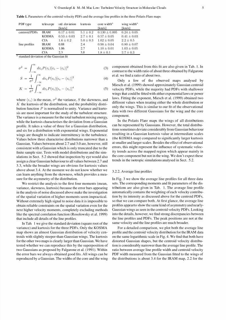
Table 1. Parameters of the centroid velocity PDFs and the average line profiles in the three Polaris Flare maps

PDF type telescope std. deviation kurtosis core widtha wing widtha

[km/s] [km/s] [km/s]

centroid PDFs IRAM 0.17± 0.01 5.1± 0.2 0.130± 0.005 0.24± 0.05

KOSMA 0.53± 0.03 2.7± 0.1 0.57± 0.05 0.41± 0.03

CfA 1.6± 0.2 5.0± 0.3 1.02± 0.05 2.2± 0.5line profiles IRAM 0.88 2.4 0.98± 0.04 0.80± 0.07

KOSMA 1.06 2.7 1.10± 0.01 1.03± 0.05

CfA 2.3 3.8 1.8± 0.1 2.7± 0.3

a standard deviation of the Gaussian fit

σ2 =

∞−∞

dvcP (vc)[vc − vc]2 (3)

S =1

σ3

∞−∞


K =1

σ4

∞−∞


where vc is the mean, σ2 the variance, S the skewness, and

K the kurtosis of the distribution, and the probability distri-

bution function P is normalised to unity. Variance and kurto-

sis are most important for the study of the turbulent structure.The variance is a measure for the total turbulent mixing energy,

while the kurtosis characterises the deviation from a Gaussian

profile. It takes a value of three for a Gaussian distribution,

and six for a distribution with exponential wings. Exponential

wings are thought to indicate intermittency in the turbulence.

Values below three characterise distributions narrower than a

Gaussian. Values between about 2.7 and 3.0 are, however, still

consistent with a Gaussian which is only truncated due to the

finite sample size. Tests with model distributions and the sim-

ulations in Sect. 5.2 showed that inspection by eye would also

assign a clear Gaussian behaviour to all values between 2.7 and

3.3, while the broader wings are obvious for kurtosis values

above about 3.4. At the moment we do not know whether we

can learn anything from the skewness, which provides a mea-

sure for the asymmetry of the distribution.

We restrict the analysis to the first four moments (mean,

variance, skewness, kurtosis) because the error bars appearing

in the analysis of noise discussed above make the investigation

of the spatial variation of higher moments seem impractical.

Without extremely high signal to noise data it is impossible to

obtain reliable constraints on the spatial variation even for the

next higher velocity moments, completely excluding methods

like the spectral correlation function (Rosolowsky et al. 1999)

that include all details of the line profiles.

In Tab. 1 we give the standard deviation (square root of thevariance) and kurtosis for the three PDFs. Only the KOSMA

map shows an almost Gaussian distribution of velocity cen-

troids with slightly steeper-than-Gaussian wings. The kurtosis

for the other two maps is clearly larger than Gaussian. We have

tested whether we can reproduce this by the superposition of

two Gaussians as proposed by Falgarone et al. (1991). Within

the error bars we always obtained good fits. All wings can be

reproduced by a Gaussian. The widths of the core and the wing

component obtained from this fit are also given in Tab. 1. In

contrast to the width ratio of about three obtained by Falgarone

et al. we find a ratio of about two.

Only a few of the observed maps analysed by

Miesch et al. (1999) showed approximately Gaussian centroid

velocity PDFs, while the majority had PDFs with shallower

wings that could be fitted with either exponential laws or power

laws. Fitting the exponent, Miesch et al. (1999) obtained two

different values when treating either the whole distribution or

only the wings. This is similar to our fit of the observational

data with two different Gaussians for the wing and the corecomponent.

In the Polaris Flare maps the wings of all distributions

can be represented by Gaussians. However, the total distribu-

tions sometimes deviate considerably from Gaussian behaviour

resulting in a Gaussian kurtosis value at intermediate scales

(the KOSMA map) compared to significantly larger kurtosis

at smaller and larger scales. Besides the effect of observational

errors, this might represent the influence of systematic veloc-

ity trends across the mapped region which appear mainly in

the core component but not in the wing. We don’t expect these

trends in the isotropic simulations analysed in Sect. 5.2.

3.2.2. Average line profiles

In Fig. 3 we show the average line profiles for all three data

sets. The corresponding moments and fit parameters of the dis-

tributions are also given in Tab. 1. The average line profile

automatically contains the weighting of each velocity contribu-

tion by its intensity as discussed above for the centroid PDFs,

so that we can compare both. At first glance, the average line

profiles appearto show the same kind of asymmetry and nearly-

Gaussian wings as seen in the centroid velocity PDFs. Looking

into the details, however, we find strong discrepancies between

the line profiles and PDFs. The peak positions are not at the

same velocity and the line profiles are much broader.For a detailed comparison, we plot both the average line

profile and the centroid velocity distribution for the IRAM data

on the same logarithmic scale in Fig. 4. We find that both have

distorted Gaussian shapes, but the centroid velocity distribu-

tion is considerably narrower than the average line profile. The

ratio between average line profile width and centroid velocity

PDF width measured from the Gaussian fitted to the wings of

the distributions is about 3.4 for the IRAM map, 2.2 for the




Fig. 2. Probability density distribution of centroid velocities for the

three Polaris Flare data cubes. The error bars show the deviation intro-

duced by different treatments of the observational noise, as discussed

in the text.

KOSMA map, and 1.5 for the CfA map. Using the variance of

the full distributions we get ratios of 5.2, 2.0, and 1.4 respec-

tively for the three maps. The difference of the two ratios for

the IRAM map corresponds to some large scale velocity flow

on that scale producing the irregular PDF core seen in Fig. 4.

Fig. 3. Average line profiles for the three Polaris Flare data cubes. The

solid line shows the IRAM data, the dotted line the average profile in

the KOSMA map multiplied by 2 and the dashed line the CfA data

multiplied by 8.

Fig. 4. Comparison of the total velocity PDF given by the average line

profile and the centroid velocity PDF for the IRAM data.

The variation of this ratio with the size of the map is again

naturally explained by the two different length scales involved:

the line-of-sight integration and the size of the map. In the

IRAM data, the small size of the map provides a relatively nar-

row centroid velocity PDF compared to the broad average line

profile determined by the line-of-sight integration through the

full depth of the cloud. In contrast, the thickness of the cloud

will certainly be smaller than the full extent of the CfA map.

This is also indicated by the approaching slopes of the twodifferent variances within beams of varying size in Fig. 1 at

large scales. To compare the ratios obtained here with turbu-

lence simulations in model cubes we have to consider scales

where the map size is about equal to the thickness of the cloud.

From the intensity maps of the clouds and Fig. 1 we estimate

a thickness corresponding to about 2◦ in angular scale. The re-

sulting typical value for the width ratio that we should repro-

duce in the turbulence simulations then falls between about 1.5




and 1.6. We will see that several but not all turbulence models

show such values.

We can resolve the long lasting dispute over whether to use

the average line profiles or the centroid velocity PDF as a mea-

sure for the 3D velocity PDF. The answer is determined by the

size scales involved in the observations. Since the velocity cen-

troids ignore the integration along the line of sight, they provide

the correct distribution only if the map size is larger or at least

comparable to the thickness of the cloud. For small maps, the

line profiles provide the better average, because they include alarger sample from the larger line-of-sight integration.

We have to mention that this conclusion can be distorted

by two other effects that might be responsible for differences

between average line profiles and centroid PDFs. First, the op-

tical depth of the 12CO transitions will typically increase the

observed linewidth relative to the total velocity distribution. It

reduces the core of the average line profile more than that of the

centroid PDF. However, Bensch et al. (2000a) have found that

the 13CO and 12CO Polaris data show the same spatial scal-

ing laws, although the maps differ. Hence, we will assume here

that optical depth effects play only a minor role. Comparison

with the simulations in Sect. 5.2 show that, although they werenot measured in an optically thin transition, the average line

profiles taken from the Polaris Flare data seems to be a better

indicator for the true velocity PDF than the centroid PDF.

Second, we consider different directions for tracing the ve-

locity distribution with the two methods. They only provide the

same results for a perfectly isotropic medium. We must con-

clude that both distributions provide partially complementary

information so that a combined treatment is necessary.

3.3. Velocity difference PDFs

From the velocity centroid maps one can also extract informa-tion on the distribution of scales in the velocity field by consid-

ering PDFs of velocity differences between points separated by

different lags (distances). This provides independent informa-

tion on the structure of the velocity field. Investigation of the

PDF of velocity differences as a function of spatial separation

has been pursued by Miesch & Scalo (1995), Lis et al. (1998),

and Miesch et al. (1999). For a discussion of the details and the

application to several molecular clouds we refer to Miesch et

al. (1999).

Here we don’t study the full PDF of centroid velocity dif-

ferences but the variation of the first statistical moments of this

PDF as a function of lag between the two points considered.

Because of the symmetry of the velocity differences, all oddmoments vanish. The first two non-zero moments of the veloc-

ity difference distribution are the variance and the kurtosis:

σ2(L) =

map

d2r

|r−r

|=L

d2r f (r)f (r) [vc(r) − vc(r)]2

map

d2r

|r−r

|=L

d2r f (r)f (r)(6)

Fig. 5. The standard deviation of the velocity difference PDF as a func-

tion of lag.

K (L) =

map

d2r

|r−r

|=L

d2r f (r)f (r) [vc(r) − vc(r)]4

σ4

(L) map

d2

r |r−r

|=Ld2

r

f (r)f (r

)

. (7)

Integrations over the spatial vectors r and r scan the whole

map. The contribution of the velocity difference between the

points r and r is weighted by weighting factors f . As dis-

cussed above, the selection of appropriate weighting factors is

already difficult for the centroid PDFs, and becomes even more

complex for the velocity difference PDFs, because each term in

the integral contains contributions from two points. We have

tested three different weighting factors: a) equal weighting,

with f (r) = 1 for all points above the noise limit (the weight-

ing used by Miesch et al. 1999); b) weighting by the geometric

mean of the two intensities; and c) weighting by the product of

the two intensities. We have performed numerous tests for the

observational data and turbulence models and found no essen-

tial differences in the resulting spatial variation of the velocity

difference PDF moments apart from a different noise level. In

the following we use the weighting by the geometric mean, as

it is a linear intensity weighting for each term, as in the case of

the PDFs discussed above.

The quantity given by the variance of the two-point PDF

σ2(L) in Eq. (6) as a function of the lag between the points

L is identical to the ordinary structure function as used e.g.

by Miesch & Bally (1994), except for the normalisation of the

structure function, so we can compare the results. Miesch et al.

(1999) obtained for several clouds a power law behaviour forthe variance of the centroid velocity differences σ2(L) ∝ Lγ ,

with γ ≈ 0.85 (0.33 . . . 1.05) except for the largest lags, where

σ2 remained roughly constant. To enable a better comparison

with the size-linewidth relation discussed above, we use here

the standard deviation σ instead of the variance σ2. In Fig. 5

we show the resulting plot for the Polaris Flare data. We find

an overall slope of 0.47, quite close to that found for the size-

linewidth relation. The error bars are somewhat smaller but the




Fig. 6. The kurtosis of the centroid velocity difference PDF as a func-

tion of the lag between the points considered.

two data sets at higher resolution show some decrease of the

slope at the largest lag. This must be an artifact due to the finite

map size, since it does not continue at the next larger scale. The

structure functions calculated by Miesch et al. (1999) show amuch stronger flattening at large lags, going to constant values

for all maps. This is probably due to the artificial removal of

velocity structure at large lags introduced by their method to

subtract large scale trends.

The good agreement between the size-linewidth relation for

the centroid velocities in Sect. 3.1 and the structure function

discussed here seems inevitable when we consider that the vari-

ance in velocity differences on a certain scale is a kind of differ-

ential measure for the total variance within a certain radius as

measured with the scanning-beam size-linewidth relation. We

thus expect a similar behaviour.

The kurtosisK (L)

is a measure for the Gaussian behaviour

of the velocity differences and thus for the correlation of the

internal motions. Uncorrelated velocities provide a Gaussian

distribution of differences characterised by a kurtosis of three.

Hence, we expect this value when considering points separated

by a large lag. Values of the kurtosis exceeding three at differ-

ent lags provide a measure for the strength of the correlations in

velocity space at those scales. Miesch et al. (1999) found that

the velocity difference PDFs in the studied clouds change from

kurtosis values between about 10 and 30 at small lags to nearly

Gaussian behaviour at large lags. This is also typical for in-

compressible turbulence (She (1991)). Lis et al. (1998) found

strong non-Gaussian distributions at scales associated with fil-

aments and approximately Gaussians at larger lags.In Fig. 6 the kurtosis of centroid velocity differences in the

Polaris Flare data is plotted. In contrast to the other quantities,

the different resolutions do not line up here to a single line but

the kurtosis for each map drops independently to the Gaussian

value at about the map size. This behaviour can be understood

by considering which quantities at which scales determine the

kurtosis. At the largest lag of any map the kurtosis measures

mainly the shape of the centroid probability distribution of the

whole map which is more or less close to Gaussian for all data

sets considered here (Sect. 3.2.2). Thus we can always expect

a value around 3 when the scale for the kurtosis determination

approaches the map size. Contrary to the discussion provided

by Miesch et al. (1999), this does not mean that there are no

correlations at larger scales but that they cannot be addressed

from points within the map.

At all smaller lags the kurtosis is a measure for the corre-

lated motions on that scale relative to the overall motions seen

in the map, which is scanned when computing the kurtosis andvariance. In Sect. 3.3 we will see that kurtosis values above

three are produced only if the maps contain some motion on

scales larger than the scale on which the kurtosis is measured.

The steps in Fig. 6 are thus unavoidable when switching to an-

other map since we always measure the correlated motions on

a particular scale relative to the total motions in the map con-

sidered. A slightly sub-Gaussian behaviour at the largest scale

might be produced by optical depth effects somewhat flattening

the core of the distribution.

3.4. The ∆-variance

Stutzki et al. (1998) introduced the ∆-variance to measurethe amount of structure present at different scales in multi-

dimensional data sets. The ∆-variance at a given scale of an

n-dimensionaldata set is computed by convolving the data with

an n-dimensional spherical down-up-down function of that

scale, and measuring the remaining variance. The ∆-variance

analysis computes the average variance on a certain scale sim-

ilar to the structure function giving the variance of the velocity

differences between two distinct points separated by a certain

lag. For the ∆-variance, however, the variance of the filtered

map is computed, instead of the average variance of all point-

to-point differences corresponding to a certain lag. Thus, the

∆-variance of a smooth map with a linear gradient vanishes,

while the structure function discussed above detects the gradi-

ent. The advantage of the ∆-variance is its better sensitivity to

specific spatial scales. It provides a good separation of system-

atic trends, structures on certain scales, and effects like noise.

Furthermore, it allows the direct computation of the equivalent

Fourier spectral index. A comprehensive discussion is given

by Bensch et al. (2000a). A similar method was introduced re-

cently by Brunt (1999) to characterise the 3D velocity structure

of model cubes. He used a rectangular filter function composed

of adjacent cubes of different size rather than the spherically

symmetric filter function used to compute the ∆-variance.

Bensch et al. (2000a) applied the ∆-variance analysis to

the intensity maps of the Polaris Flare discussed above. Weused the same method in paper I to analyse the density struc-

ture in turbulence simulations, and compared the results to the

observational data. Paper I also discussed the ∆-variance for

the 3D velocity field of the simulated turbulence and compared

it to the ∆-variance for the 3D density, but did not provide any

direct comparison to the observations. We found that the ∆-

variance of the velocity behaves similarly to that of the density

in showing the characteristic scale of the driving mechanism




Fig. 7. The square root of the ∆-variance of the velocity centroid maps

of the Polaris Flare observations.

used in the turbulence models. However, the amount of struc-

ture observed at smaller scales differs between density and ve-

locity. The turbulence creates many thin dense regions, leading

to an exponent of the ∆-variance for the density of about 0.5,whereas it creates hardly any small-scale structures in the ve-

locity field, so that the ∆-variance for the velocity drops off

much more steeply, with an exponent of about 2.

Unfortunately this method of measuring the structure of the

3D velocity field in the simulations has no directly equivalent

approach applicable to observations, since they only provide

one-dimensional velocity information projected onto the plane

of the sky. There exists no simple relation between the three

dimensional velocity structure and the behaviour of the projec-

tions. Therefore, we must instead apply the ∆-variance analy-

sis to observable velocity parameters like the map of centroids

which can be derived from both the simulations and the obser-

vations. They can be used to judge whether a simulation re-

produces observed properties. We do lose information by this

procedure, of course.

Fig. 7 shows the square root of the ∆-variance for the Po-

laris Flare velocity centroid maps. In contrast to paper I, we

have chosen to take the square root, yielding the standard de-

viation of the filtered maps instead of the variance, in order to

give a better comparison to the other linewidth related quanti-

ties. The upturn at the smallest scales in each map is produced

by noise in the maps which is only clearly detected by the ∆-

variance. Bensch et al. (2000a) showed how the influence of

noise can be subtracted in the ∆-variance. We have corrected

for the noise by smoothing the velocity centroid maps with aGaussian filter the size of which was adjusted in such a way

that the resulting ∆-variance shows the same behaviour as the

∆-variance where the noise was removed following Bensch et

al. We were then also able to apply the other analysis methods

to the smoothed maps to test their sensitivity to noise in the

maps.

Fig. 8 shows the resulting ∆-variance plot. In contrast to

Fig. 7, we find a turn-down at the smallest lags in each map,

Fig. 8. The square root of the ∆-variance of the smoothed Polaris Flare

velocity centroid maps. The size of the smoothing filter was adapted

to remove only the average noise level.

which is due to the finite beam size of the observations and

was hidden in the noise level before the noise correction. Un-

fortunately, it is impossible to correct for both effects simulta-

neously (Bensch et al. 2000a). In each map the beam smearing

somewhat reduces the ∆-variance at the three points for the

smallest lags, but we can clearly see that without that reduc-

tion, the ∆-variances line up well to form a continuous func-

tion with approximately a power-law behaviour at small and

intermediate scales. The slope falls between 0.7 at the smallest

scales and 0.46 in the intermediate-scale KOSMA map. Simi-

lar values for the slope of the ∆-variance at the different scales

were found for the intensity maps by Bensch et al. (2000a).

Over most scales covered by the CfA map, the slope flat-tens to zero, in contrast to the behaviour in the intensity maps.

This virtual lack of large-scale variations does not reflect the

real structure but appears due to the missing weighting in the

∆-variance analysis. Here, all points are counted equally, even

those with intensities well below the noise limit. Thus, the ∆-

variance analysis necessarily fails in cases where the maps are

only sparsely filled by emission. Less than one third of the CfA

map shows emission above the noise limit so that we cannot ex-

pect any significant results at scales above half a degree. For the

maps at smaller scales without large “empty” regions, we note

that in contrast to the size-linewidth relation and the structure

function, we find a significant change in the slope on different

scales.

The analysis of the noise-corrected maps using the other

methods discussed above showed no strong changes. The size-

linewidth relation and the structure function of the velocity cen-

troids exhibit a weak steepening of the slope by about 0.04,

while the velocity PDFs and the kurtosis show no clear differ-

ences. These methods appear to not be particularly sensitive to

changes at any single scale.




3.5. Comparison of the methods

We can classify all of the methods we have described in terms

of the velocity information setup in a two-dimensional map,

the filtering function used, and the weighting of the data in the

map.

Most analyses were restricted to the velocity centroids,

which are effectively the first moment of the local velocity pro-

file. The size-linewidth relation adds the local variance, i.e. the

second velocity moment, and the study of the PDFs also usesthe kurtosis. Higher moments become increasingly uncertain

due to the influence of observational noise, non-perfect spec-

tral baselines, and error-beam pickup (see e.g. Bensch et al.

2000b). However, with sufficiently high signal-to-noise, higher

moments may provide valuable additional information.

The variance is strongly dominated by the depth of the ob-

served cloud, so that it contains information lost when consid-

ering the velocity centroids only. We have seen that, for maps

where the line profiles sample the cloud deeply in comparison

to the map size, the integrated line profile is a better measure

for the true velocity distribution function than the PDF of the

velocity centroids.

We have applied three different kinds of filters: thescanning-beam size-linewidth relation effectively convolves

the map with a positive Gaussian filter; the ∆-variance anal-

ysis uses a spherically symmetric up-down filter; and the struc-

ture function uses a filter consisting of a positive and a neg-

ative spike separated by a certain distance. In the latter case,

spherical symmetry is provided by the superposition of the

resulting variance values for different directions of the filter

axis. The structure function is sensitive to large-scale gradi-

ents and can detect certain geometric structures, but because

of the strong localisation of the filter in the spatial domain, it

is unfortunately sensitive to a broad spectrum of spatial fre-

quencies in the Fourier domain. In the statistical analysis of

velocity fluctuations, it is therefore at a disadvantage in the

detection of characteristic scales and frequencies compared to

the ∆-variance analysis. Similar conclusions were obtained by

Houlahan & Scalo (1990).

The ∆-variance analysis, on the other hand, does not yet

take into account different weights for the information in dif-

ferent regions of an observed map, so that it fails for maps with

large regions dominated by noise. The weighting of the veloc-

ity centroid information by the intensity, as is done automati-

cally in the size-linewidth relation, reduces the uncertainty due

to observational noise when computing the centroid probability

distribution or structure function.

3.6. Other approaches

With sufficiently high signal-to-noise ratio, it is possible to

extend the methods discussed here. Overviews of the differ-

ent existing methods have been provided recently by Vazquez-

Semadeni (2000) and Ossenkopf et al. (2000). First, one can ap-

ply the basically two-dimensional methods to higher moments

of the line profiles, providing new information especially on

the intermittency in velocity space. Alternatively, the velocity

channel maps can be analysed as demonstrated with the ∆-

variance analysis by Ossenkopf et al. (1998). Another method

is to compare full spectra, using the spectral correlation func-

tion (Rosolowsky et al. 1999) and extending this method to

consider all spatial variations.

Tauber (1996) discussed the smoothness of line profiles as a

measure for the size and number of coherent units contributing

to the profiles. Applying a rough approximation to this analy-

sis, Falgarone et al. (1998) conclude that the size of cells in thePolaris Flare observations must be as low as 200 AU.

When looking for characteristic global features in the

density-velocity structure, the principal component analysis in-

troduced by Heyer & Schloerb (1997) is probably the most sig-

nificant tool. It identifies the main components in the position-

velocity space in terms of eigenvectors and eigenimages. Al-

though the principal component analysis represents a reliable

method to find the dominant structures even in complicated im-

ages, the significance of the higher-order moments still has to

be determined.

4. Turbulence models

4.1. Simulations

We use simulations of uniform decaying or driven turbulence

with and without magnetic fields described by Mac Low et

al. (1998) in the decaying case and by Mac Low (1999) in

the driven case. These simulations were performed with the

astrophysical MHD code ZEUS-3D2 (Clarke (1994)). This is

a 3D version of the code described by Stone & Norman

(1992a,b) using second-order advection (van Leer (1977)),

that evolves magnetic fields using constrained transport

(Evans & Hawley (1988)), modified by upwinding along shear

Alfven characteristics (Hawley & Stone (1995)). The code

uses a von Neumann artificial viscosity to spread shocks out tothicknesses of three or four zones in order to prevent numerical

instability, but contains no other explicit dissipation or resistiv-

ity. Structures with sizes close to the grid resolution are subject

to the usual numerical dissipation, however. In Paper I we dis-

cussed the effects of limited numerical resolution, which leads

to numerical viscosity, and noted that resolution studies could

be used to determine which properties were well resolved.

The simulations used here were performed on a 3D, uni-

form, Cartesian grid with side L = 2 and periodic boundary

conditions in every direction, using an isothermal equation of

state. To deal with velocities comparable to those in the obser-

vations we have assumed here a cloud temperature of 10 K cor-

responding to a translation of the dimensionless sound speed inthe simulations to a physical sound speed of 0.2 km/s in the data

analysis. The initial density and, in relevant cases, magnetic

field are both initialised uniformly on the grid, with the initial

density ρ0 = 1 and the initial field parallel to the z-axis. The

2 Available from the Laboratory for Computational Astro-

physics of the National Center for Supercomputing Applications,

http://zeus.ncsa.uiuc.edu/lca home page.html




turbulent flow is initialised with velocity perturbations drawn

from a Gaussian random field determined by its power distri-

bution in Fourier space, as described by Mac Low et al. (1998).

For decaying models we use a flat spectrum with power in

the range kd = 1 − 8, where the dimensionless wavenumber

kd = L/λd counts the number of driving wavelengths λd in

the box. For our driven models, we use a spectrum consisting

of a narrow band of wave numbers around some value kd, and

driven with a fixed pattern at constant kinetic energy input rate,

as described by Mac Low (1999).We have tested the influence of numerical viscosity by run-

ning the simulations with the same physical parameters on

grids of 643, 1283 or 2563 zones. Higher resolution grids have

numerical viscosity acting at smaller scales, so changing the

resolution shows the effects of numerical viscosity on our re-

sults. The influence of numerical resolution on the simulation

results is discussed below separately for each for the statistical

measures.

4.2. Simulated Observations

To compare our simulations with observations we must syn-

thesise observational maps from the simulated density and ve-locity fields. We assume that the cubes are optically thin for

this first study so that direct integration along lines of sight

through the cube neglecting optical depth effects yields line

profiles. This appears to be a reasonable assumption for com-

parison with the low column density clouds in the Polaris flare

observed in 13CO, but is a worse assumption for higher column

density clouds or more optically thick species.

We also neglect the periodic nature of the simulations, ef-

fectively observing the simulation cubes as isolated structures

in a vacuum. This second assumption must be taken into ac-

count in analyses affected by the path-length through the cloud,

such as comparisons of the velocity PDF measured from the

average line profile vs. the centroid velocity distribution.

4.3. Statistical fluctuations

To get a feeling for the significance of the structural proper-

ties indicated by the different measures relative to the statistical

variations in the turbulence we can compare differentdirections

within the same model cube. In a decaying turbulence simula-

tion any anisotropies introduced by the random initial driving

should be suppressed after several turn-over times so that we

expect about the same statistical behaviour in each direction.

Fig. 9 shows the ∆-variances and structure functions for the

three centroid velocity maps obtained by projecting a modelcube of decaying hydrodynamic turbulence along the three dif-

ferent axes onto the virtual plane of the sky. In the ∆-variance

plots we always give the the standard deviation (the square root

of the ∆-variance) instead of the variance for a better compar-

ison to the other velocity variations.

The ∆-variances show the same general behaviour in each

direction, with a range of clearly visible variations in the rela-

tive contributions at large lags, where the exact modal structure

Fig. 9. ∆-variances (upper panel) and structure functions (lower

panel) in the centroid velocity maps obtained for a decaying hydro-

dynamic model (model D from Mac Low et al. (1998)) in the three

possible directions of projection. The dotted line indicates a slope of

0.5 for comparison. The variation between the different directions is

similar for the other models.

is still different in the three directions. These differences are

also directly visible to the eye of an experienced user in the

centroid velocity maps. The structure function shows smaller

variations corresponding to its lower sensitivity to changes at

particular spatial frequencies. The variation of the slope in the

different directions falls below 0.1.

The equivalent plot for the size-linewidth relation is simi-

lar to that for the structure function. The variations in the kur-

tosis, on the other hand, are more like those seen in the ∆-

variance. Here, we sometimes find small dips and rises distort-

ing the monotonicdecay to values slightly below3 at the largestscales, indicating marginally sub-Gaussian distributions there.

In the total and the centroid velocity PDFs we find remarkable

variations in the core and the central position of the distribu-

tions corresponding to the different largest velocity modes but

no changes in the wing behaviour.

The model used for demonstration here is typical for most

of the simulations performed. Therefore variations by up to a

factor 1.4 in the square root of the ∆-variance at certain lags




Fig.10. Size-linewidth relation for the velocity centroids of a hydro-

dynamic simulation driven at wavenumbers of kd = 2 (solid), kd = 4

(dashed), and kd = 8 (dot-dashed). These are models HE2, HE4, and

HE8 from Mac Low (1999). The dotted line shows a power-law with

slope 0.5.

and by 0.05 in the slope of the autocorrelation function and thesize-linewidth relation can be considered as statistical fluctua-

tions within a model that should be excluded from a discussion

of significant differences between the models.

5. Statistical description of simulations and comparison to

observations

5.1. Size-linewidth relation

We begin by considering the results of applying the size-

linewidth analysis described in Sect. 3.1 to the models. In

Fig. 10 we show the size-linewidth relation for the velocity

centroids in three models of hydrodynamic driven turbulence

that differ only in the scale that they are driven. The driving

wavelengths are 1/2, 1/4, and 1/8, respectively.

We find power-law behaviour through most of the regime

only for the model driven at the largest available scales. Models

driven with smaller characteristic scales show a flattening of

the relation at lags above the driving scale. A slight flattening

at the largest lags is also visible in the observational data. This

appears to be an indication of a turbulence driving scale close

to the size of the molecular cloud.

A drop off in velocity dispersion is seen at small lags in

all of the models. This can be explained straightforwardly as

an effect of numerical viscosity. In Fig. 11 we show a compar-

ison of three models of decaying turbulence that are statisti-cally identical, but were computed at resolutions of 643, 1283,

and 2563 zones. Increasing resolution results in decreasing nu-

merical viscosity, so Fig. 11 demonstrates explicitly the effect

of changing the numerical viscosity. As can be seen, the slope

does not change at large lags, and the higher resolution mod-

els agree within a few percent on the magnitude of the velocity

dispersion. At small lags, on the other hand, the velocity dis-

persion falls off. This occurs in all models at roughly the same

Fig.11. Size-linewidth relation for the velocity centroids in a hydrody-

namic simulation of decaying turbulence at time t = 0.75tcross (tcrossis the initial crossing time of the region), computed at resolutions of

643 (dot-dashed), 128

3 (dashed), and 2563 (solid). These are models

B, C, and D from Mac Low et al. (1998).

number of grid zones, and hence at larger physical scale inthe lower resolution models. This part of the spectrum thus re-

flects the effect of numerical diffusion eliminating some of the

small-scale structure. The same drop-off occurs in each model

(see Fig. 10), so the behaviour at the smallest scales should be

viewed with caution. We note, however, that a physical diffu-

sion such as ambipolar diffusion (Zweibel & Josafatsson 1983,

Klessen et al. 2000) is expected to produce similar behaviour

at the diffusion scale.

Magnetic fields do not appear to modify the size-linewidth

relation, although they can make order unity differences in the

magnitude of the velocity dispersion and produce significant

anisotropy, as described below in Sect. 5.4.

We can conclude that the observed power-law behaviour

of the size-linewidth relation is reasonably explained by either

hydrodynamic or magnetised turbulence driven at scales com-

parable to the largest observed scales.

5.2. Velocity probability distribution function

We have access to the full 3D velocity field in the computa-

tional models, and so can compare the actual PDFs to the PDFs

measured in various ways from simulated observations of that

model. In this way, we hope to gain insight into the physical

conditions that generate the observed PDFs discussed in Sect.

3.2 and 3.3.

5.2.1. Centroid velocity PDFs

First, we examine the effect of numerical resolution on the cen-

troid velocity PDFs. In Fig. 12 the 3D PDFs are compared to

the centroid PDFs for a model of decaying MHD turbulence at

different resolutions. All PDFs are well represented by Gaus-

sians. The width of the PDF drops at smaller resolution. This




Fig.12. (a) 3D and (b) centroid velocity PDFs in a model of strongly

magnetised decaying turbulence with initial Mach numberM = 5 and

Alfven number A = 1 after 1.5tcross at a resolution of 2563 (solid),

1283 (dashed), and 643 (dashed-dotted). (Models Q, P, N from Mac

Low et al. 1998)

can be attributed to the stronger influence of the numerical vis-

cosity in the lower resolution cubes damping the turbulence

faster. This agrees with the measurements of resolution effects

on kinetic energy described in Mac Low et al. (1998), in which

the magnitude of the kinetic energy increased with resolution,

although the decay rate was constant. An additional effect is

seen in the centroid PDFs. At low resolutions the sampling of

the wings of the Gaussian is insufficient, so that the distribu-

tion appears too narrow. The kurtosis values of these PDFs are

2.6, 2.8, and 2.9 with growing resolution. Hence, sub-Gaussian

kurtosis values can at least partially be explained by small mapsizes.

In Table 2 we give the PDF momentsfor most of the models

discussed, covering a wide range of different physical proper-

ties. The first several columns describe the model input param-

eters, and the remaining columns contain the parameters of the

PDFs obtained.

We first consider the effect of varying the driving

wavenumber, holding the energy input constant. Fig. 13 and the

Fig.13. Centroid velocity PDFs from three models driven with the

same strength at wavenumbers of kd = 2 (solid), kd = 4 (dashed),

and kd = 8 (dash-dotted) (models HC2, HC4, and HC8 from Mac

Low 1999)

corresponding values in Table 2 show that driving at smaller

wavenumbers (longer wavelengths) produces broader PDFs,because such models have lower dissipation rates (Mac Low

1999), and thus higher rms velocities. More interestingly, we

find that driving at the largest scale in the model kd = 2 pro-

duces a centroid velocity PDF with apparently non-Gaussian

shape, as reflected in the kurtosis value of 2.4 given in Table 2.

A similar result was found by Klessen (2000), who argued that

it is most likely due to cosmic variance. That is, an insuffi-

cient number of modes are sampled at these long driving wave-

lengths to fully describe a Gaussian field, so the PDF appears to

have a distortedshape. Dependingon the random numbers used

to initialise the largest modes, both Gaussian and non-Gaussian

kurtosis values are then possible.

To demonstrate the effect of magnetic fields, Fig. 14 shows

the centroid velocity PDFs from a model of decaying magne-

tised turbulence. It clearly indicates an anisotropic decay, with

velocity components perpendicular to the magnetic field de-

caying substantially more quickly than velocities parallel to the

field. In both cases, though, the PDFs remain Gaussian even at

late times. These conclusions are quantitatively supported by

Table 2.

In Fig. 15, we examine magnetised driven turbulence. The

fields do shift the peak back and forth slightly, but, as shown

in Table 2, they still produce only slightly non-Gaussian cen-

troid velocity PDFs in cases where the hydrodynamic model

is Gaussian, contrary to the speculation of Klessen (2000) thatmagnetic fields might be an important alternative cause of non-

Gaussian PDFs. The PDFs observed parallel to the field are

roughly 20% wider than the perpendicular observations shown

in Fig. 15.

Klessen (2000) showed that driving from large scales can

produce non-Gaussian PDFs, but worried that every additional

piece of physics also appeared likely to produce non-Gaussian

PDFs, allowing no conclusions to be drawn from their oc-




Table 2. Parameters of the centroid velocity PDFs and the total velocity PDFs for the model cubes

modela Lb kcd

N d M e vA

cs

f tg σ2

c2s

(cen)h σ2

c2s

(cube)hσ2(cube)σ2(cen) K (cen) j K (cube) j

HA8 0.1 7–8 128 1.9 0 1.0 3.6 10 2.8 3.0 2.9

HC2 1 1–2 128 7.4 0 1.0 50 55 1.1 2.4 2.5

HC4 1 3–4 128 5.3 0 1.0 17 31 1.8 3.2 2.7

HC8 1 7–8 128 4.1 0 1.0 9.4 22 2.3 3.6 3.0

HE2 10 1–2 128 15 0 0.98 49 76 1.6 3.0 2.7

HE4 10 3–4 128 12 0 0.88 38 67 1.8 2.9 3.0

HE8 10 7–8 128 8.7 0 1.0 21 47 2.2 3.9 3.0MA4X: v⊥ 0.1 3–4 128 2.7 10 0.3 7.0 14 2.0 2.6 2.8

v 0.1 3–4 128 2.7 10 0.3 10 16 1.6 3.4 3.3

MC4X: v⊥ 1 3–4 128 5.3 10 0.1 15 26 1.7 3.8 3.6

v 1 3–4 128 5.3 10 0.1 18 29 1.6 3.3 3.3

MC45: v⊥ 1 3–4 128 4.8 5 0.2 13 23 1.8 4.1 3.4

v 1 3–4 128 4.8 5 0.2 16 29 1.8 3.1 3.0

MC41: v⊥ 1 3–4 128 4.7 1 0.5 15 28 1.9 3.0 2.8

v 1 3–4 128 4.7 1 0.5 13 24 1.8 3.1 3.0

MC85: v⊥ 1 7–8 128 3.4 5 0.075 6.3 15 2.4 4.1 3.8

v 1 7–8 128 3.4 5 0.075 9.0 21 2.3 3.2 3.5

MC81: v⊥ 1 7–8 128 3.5 1 0.23 6.6 19 2.9 3.3 3.1

v 1 7–8 128 3.5 1 0.23 8.5 20 2.4 3.3 3.2

ME21k: v⊥ 10 1–2 128 14 1 0.5 47 61 1.3 2.8 2.9

v 10 1–2 128 14 1 0.5 83 97 1.2 3.3 3.2B 0 1–8 64 5 0 0.1 2.7 7.0 2.6 2.6 2.9

0 1–8 64 5 0 0.3 1.9 4.0 2.1 2.8 2.9

C 0 1–8 128 5 0 0.1 2.8 7.7 2.8 3.0 3.1

0 1–8 128 5 0 0.3 1.7 4.4 2.6 3.2 2.9

0 1–8 128 5 0 0.5 1.3 3.5 2.7 2.7 2.7

D 0 1–8 256 5 0 0.1 2.9 8.4 2.9 3.0 2.9

0 1–8 256 5 0 0.3 1.9 5.0 2.6 2.9 2.9

0 1–8 256 5 0 0.5 1.4 3.8 2.7 2.4 2.9

Uk 0 1–8 256 50 0 0.1 9.1 15 1.6 2.3 2.9

0 1–8 256 50 0 0.3 6.1 8.9 1.5 2.1 2.6

0 1–8 256 50 0 0.5 5.0 7.0 1.4 2.1 2.5

Q: v⊥ 0 1–8 256 5 5 0.1 3.6 11 3.1 3.2 3.3

0 1–8 256 5 5 0.3 2.4 6.4 2.7 2.9 3.3

0 1–8 256 5 5 0.5 2.1 4.9 2.3 3.0 3.2Q: v 0 1–8 256 5 5 0.1 4.7 9.5 2.0 2.9 3.0

0 1–8 256 5 5 0.3 3.9 6.3 1.6 3.0 3.4

0 1–8 256 5 5 0.5 3.4 4.9 1.4 3.1 3.3

a Driven models (H & M series) from Mac Low (1999); decaying models (single letters) from Mac Low et al. (1998).b Mechanical driving luminosity in arbitrary units (see Sect. 2.3 of Mac Low (1999) for all unit conversions).c Driving wavenumber.d Number of zones in each dimension.e rms Mach number: initial value for decaying models, equilibrium value for driven models.f Ratio of Alfven velocity to sound speed.g Time at which values are measured, in sound-crossing times.h Variance of distribution for line centroid velocities and full cube. j

Kurtosis of distribution for line centroid velocities and full cube.k Unpublished model.

currence. We have, however, demonstrated that neither mag-

netic fields nor the vorticity introduced by shock interactions in

driven or decaying turbulence produce strongly non-Gaussian

PDFs. Another candidate for producing non-Gaussian PDFs is

self-gravity, but the lack of star-forming activity in the Polaris

Flare suggests that self-gravitation does not play a dominant

role there. This suggests that the non-Gaussian PDFs observed

there (Sect. 3.2) are indeed due to the cosmic variance intro-




Fig.14. Centroid velocity PDFs from a model of decaying, magnetised

turbulence (model Q from Mac Low et al. (1998)) at times in units of

the initial crossing time tcross of 0.5 (solid), 0.75 (dashed),1.5 (dash-

dot), and 2.5 (dotted) observed (a) perpendicular to the field and (b)

parallel to the field.

Fig.15. Centroid velocity PDFs from a hydrodynamic model driven

withk = 4 (solid), and three magnetised models with the same driving

and vA/cs = 10 (dash), and 1 (dash-dot). These are models HC4,

MC4X, and MC41 from Mac Low (1999), observed perpendicular to

the field.

Fig.16. Comparison of the total velocity PDF and the centroid veloc-

ity PDF for a hydrodynamic model driven with one tenth of the energy

of the example above (model HC2 from Mac Low (1999)).

duced by driving from the largest scales of the region. The

driving scale may actually be even larger than identified herebecause we have not used any information from the atomic gas

at larger scales.

5.2.2. Average line profiles

Using the turbulence simulations we can now revisit the ques-

tion from Sect. 3.2.2 of how best to measure the actual 3D ve-

locity PDF from observations. In Fig. 16 we compare the PDF

of the whole velocity distribution that would be measured as the

average line profile in an optically thin LTE medium to the PDF

of the centroid velocities for a hydrodynamic model driven at

kd = 2. This plot may be compared with Fig. 4, showing the

centroid velocity distribution and the average line profile mea-sured for the IRAM map in the Polaris Flare.

In both cases we find similar distorted Gaussian distribu-

tions, with the centroid velocity distribution narrower than the

full velocity distribution. Tab. 2 contains the ratio between the

widths of the two distributions for all models. The model ratios

show substantial variation around a typical value of about two.

The strongest systematic variation appears to be with initial or

driven rms Mach number M 0, with higher M 0 giving lower ra-

tios, down to as low as 1.1 for the most strongly driven model

HE2. Observing parallel to the field lines leads to somewhat

lower ratios than perpendicular, presumably due to the higher

velocity variance seen along parallel lines of sight. However,the ratio also decreases during the decay of turbulence for un-

clear reasons.

The ratio between depth and width is fixed to unity in the

model. From the combination of the three Polaris Flare maps

we estimate in Sect. 3.2.2 a typical width ratio between 1.5

and 1.6 for a depth comparable to the lateral extension. In Fig.

16, showing a very high M 0 simulation, the ratio is 1.5, but for

the majority of simulations we find ratios of over 1.8, suggest-




Fig.17. Standard deviation of the centroid velocity difference PDF

as a function of lag (equivalent to the structure function) normalised

to the square root of the lag for 3D velocity cubes of a hydrodynamic

simulation driven at wavenumbers of kd = 2 (solid), kd = 4 (dashed),

and kd = 8 (dot-dashed). These are models HE2, HE4, and HE8 from

Mac Low (1999).

ing that the observations are of a region containing hypersonic

turbulence with M 0 of order 10 or higher.

For most model PDFs we have tested three possible fits to

the distribution: Gaussians fitting either the whole distribution

or only the wings, and an exponential fit. Although exponen-

tial wings cannot be ruled out completely, the Gaussian fits are

clearly better. We have found this to be true for all models of

driven and decaying turbulence discussed here, as can be seen

by visual inspection of Figs. 12 to 16. This result agrees with

the Gaussian velocity PDFs found by Chappell & Scalo (1999)

for models of decaying Burgers turbulence.

5.3. Velocity difference PDFs

5.3.1. Second moments: structure function

In Sect. 3.3 we have shown that the second moment of the

centroid velocity difference PDFs, or equivalently the structure

function, is a differential measure for the size-linewidth rela-

tion, so that the same power law was found for the two func-

tions when applied to the observations. In Fig. 17 we plot the

structure function of the three models driven at different scales

whose size-linewidth relation was shown in Fig. 10.

We find significant curvature in at least one of these func-

tions at the driving scales (large lags) and at the viscous dis-

sipation scale (small lags). We expect that with sufficient dy-namic range there would be a set of lags where both functions

would show power-law behaviour, but our 1283 models have

such limited dynamic range that there is effectively no set of

lags where this is true. Comparison of Figs. 10 and 17 shows

that the structure function has slope and behaviour compara-

ble to the size-linewidth relation, but at each lag the slope of

the size-linewidth relation appears to be larger than that of the

structure function. This may be due to the different sensitiv-

Fig.18. Kurtosis of the centroid velocity difference distribution for a

hydrodynamic simulation driven at scales of kd = 2 (solid), kd = 4

(dashed), and kd = 8 (dash-dot). These are models HE2, HE4, and

HE8 from Mac Low (1999).

ity at different scales of the two functions due to the shape of their effective filter functions (Sect. 3.5). The structure func-

tion is somewhat more sensitive to the driving scale but less

sensitive to the dissipation scale than the size-linewidth rela-

tion. The combined set of observations, on the other hand, does

have enough dynamic range to be dominated by the power-law

slope, so that both functions agree in most parts of the spec-

trum.

5.3.2. Fourth moments: kurtosis

The kurtosis of the centroid velocity difference distribution can

measure correlations in the motion at certain scales. Values

around three indicate Gaussian distributions, implying motions

uncorrelated relative to the overall velocity field of the map

considered. Miesch et al. (1999) found a decay of the kurtosis

from small to large scales roughly proportional to the square

root of the scale down to a value of three at the largest scales in

their maps. In Sect. 3.3 we found somewhat shallower slopes,

and a flat Gaussian section at scales above the total cloud size

in the CfA Polaris Flare map.

In Fig. 18 we test how different driving scales in a driven

hydrodynamic model influence the resulting kurtosis plots. We

clearly see that the models driven at larger scales reach the

Gaussian value of kurtosis at larger lags, about a factor of 2

below the peak size of the driving structure indicated by the∆-variance. This suggests that motion at lags above the scale

of the driving process remains uncorrelated. At smaller lags,

our uniformly driven models show kurtosis following ∆s−1/3,

similar to the behaviour observed for the Polaris Flare maps

in Sect. 3.3. None of our models reached the kurtosis values

around 50 shown by the observations of Miesch et al. (1999),

suggesting that additional physics, especially in the driving

function, may be responsible for these high values.




Fig.19. Kurtosis of the centroid velocity difference distribution for

models driven at a scale of kd = 4 and no field (solid), weak field

(vA/cs = 1, dashed), and strong field (vA/cs = 10, dot-dashed).

These are models HC4, MC41, and MC4X from Mac Low (1999).

Varying the resolution of our simulations does not appear tomarkedly change the peak value of kurtosis, although the scale

at which that value is reached is always the smallest scale of the

simulation, suggesting that the correlated motions introduced

by dissipation are a major influence in producing non-Gaussian

velocity-difference PDFs.

Magnetic fields do change the shape of the velocity differ-

ence PDF, though not drastically. In Fig. 19 we compare mod-

els driven at kd = 4 with different field strengths to demon-

strate that increasing field strength increases the peak value of

kurtosis through the exponential value of six.

5.4. ∆-variance

InpaperI weused the ∆-variance to investigate the spatial scal-

ing of turbulent density structure. Here, we use this method to

investigate the velocity structure. In contrast to our analysis of

the observations, we have access to the full 3D structure in the

simulations.

We start by studying how changes in the resolution, and so

in the dissipation length scale, appear in the ∆-variance spec-

trum. In Figure 20 we compare models of decaying turbulence

that are statistically identical, but were computed with resolu-

tions of 643 (dash-dotted), 1283 (dashed), and 2563 (solid). The

variations at large scales (∆s > 0.1) are most likely due to sta-

tistical fluctuations rather than the changes in resolution. Theresult of systematically increasing the resolution can be seen at

small scales, as the spectrum reaches smaller scales at higher

resolution. The shape of the spectrum at the smallest scales

in each model is very similar, with only the scale changing.

This shows the range over which numerical diffusion is acting.

Above that scale, the models agree fairly well in a region that

can be considered to be the inertial range of the turbulence. We

see that, equivalent to the density structure, numerical diffusion

Fig.20. ∆-variance for the velocity centroids for 3D velocity

cubes of a hydrodynamic simulation of decaying turbulence at time

t = 0.75tcross , computed at resolutions of 643 (dot-dashed), 128

3

(dashed), and 2563 (solid). These are models B, C, and D from

Mac Low et al. (1998).

Fig.21. ∆-variances computed for 3D velocity cubes of a hydrody-

namic simulation driven with wavenumber kd = 2 (solid), kd = 4

(dashed), and kd = 8 (dot-dashed). These are models HE2, HE4, and

HE8 from Mac Low (1999).

causes a steepening of the spectrum, and that this reaches to a

scale of roughly ten zones in every model.

Now we can consider the effects of different driving wave-

lengths. Fig. 21 shows the results of the analysis for three hy-

drodynamic models driven at different scales (the ∆-variance

for the density distribution in these models is shown in Fig. 7bof paper I). We plot the square root of the ∆-variance, as that

is the quantity directly related to the linewidth. We see pro-

nounced peaks close to the driving scale at 0.5–0.6 λd. They

are even somewhat more pronounced than in the density struc-

ture of these models (paper I), because the driving process itself

is implemented in velocity space (Mac Low 1999). Below the

driving scale we find power-law behaviour with a slope of 0.57

for ∆v corresponding to a slope of 1.14 for the ∆-variance,




Fig.22. ∆-variances of the centroid velocity maps of the three mod-

els from Fig. 21, with driving wavenumber kd = 2 (solid), kd = 4

(dashed), and kd = 8 (dot-dashed).

down to the scale of the numerical viscosity at about ten pixels

(∆s ≈ 0.04 in the figure).

How does this slope compare to the expected power spec-trum? As discussed in paper I, there is a theoretical relation

between the slope of the ∆-variance α and the index ζ of

an n-dimensional power spectrum P (k) ∝ |k|−ζ given by

α = ζ − n. Please note the difference to the index ζ int of

the often used one-dimensional power spectrum P (k) that is

obtained by angular integration of P (k), ζ = ζ int + n − 1.

Hence, the slope is translated into values of 4.14 and 2.14 for ζ and ζ int, respectively. Incompressible Kolmogorov-type turbu-

lence is characterised by values of 11/3 and 5/3, respectively,

while shock-dominated velocity fields should show the Fourier

transform of a step function, i.e. values of 4.0 and 2.0, respec-

tively. The results from the simulations are quite close to the be-

haviour of shock-dominated gas, but the small deviation might

ask for further investigations.

For the density structure, we found ∆-variance slopes be-

tween 0.45 and 0.75 in projection, corresponding to ζ (not ζ int)

values between 2.45 and 2.75, considerably flatter than the

slope in the velocity structure found here. We speculate that

this is due to the compressibility of the isothermal gas mod-

elled here. The gas piles up in thin sheets and filaments, so that

the density structure has behaviour somewhere in between that

of a δ function and a step function. The Fourier transform of a

one-dimensional δ function in the density cube is characterised

by ζ = 2. The velocity on the other hand, remains uniform

for longer distances behind shocks, so that its steeper spectralslope approaches more closely the value expected for a box full

of pure step functions.

We can compare the 3D ∆-variance spectrum to that from

simulated velocity centroid maps. In Fig. 22 we show the ∆-

variance plots for the centroid velocity maps from the mod-

els shown in Fig. 21. Here, identification of the driving scale

is no longer so easy. Nevertheless, the general functional be-

haviour is similar. The broad maximum is shifted depending

Fig.23. ∆-variance of the 3D velocity structure in a decaying MHD

turbulence model at times of 0.5, 0.75, 1.5, and 2.5 initial crossing

times.

on the driving wavelength, and there is a power law range with

the slope close to 0.5. Thus, the ∆-variance of the velocity cen-

troids does seem to reflect the true cloud velocity structure, if not as clearly as the 3D spectrum. In the centroid velocities we

measure the same drift index α as in the 3D data cube, in con-

trast to the density structure where the integrating projection to

two dimensions preserves the power spectral exponent ζ , and

therefore increases the drift index α by 1 (Stutzki et al. 1998).

This conclusion also holds for the other models so that we re-

strict ourselves here to the 3D ∆-variance, noting that the ob-

servational centroid maps do not reveal the structural properties

as clearly as discussed here.

In Fig. 23 we show the ∆-variances for the 3D velocity

structure in a sequence of four time steps in the evolution of

strongly magnetised (vA/cs = 10), decaying turbulence. The

magnitude of the variance drops over time, starting from small

scales, resulting in an increase in the effective peak of the driv-

ing function and a slight increase in the effective slope of the

spectrum over time. This effect was also seen in the density

structure in paper I, and there shown to be proportional to t1/2

as predicted by Mac Low (1999).

To demonstrate the effect of magnetic fields we show in

Fig. 24 the 3D ∆-variance plots observed parallel and perpen-

dicular to the initial magnetic field in two MHD simulations

with different field strengths, compared to a corresponding hy-

drodynamic simulation. We find a substantial anisotropy in the

case of a strong magnetic field, in contrast to the hydrody-

namic simulation and weak field cases. This is visible in thefigure which shows a velocity variance substantially greater

when viewed parallel to the initial field direction (thick line)

than perpendicular to it (thin line).

The theory of incompressible MHD turbulence

(Sridhar & Goldreich 1994, Goldreich & Sridhar 1995,

Goldreich & Sridhar 1997) predicts that the perpendicular

cascade will be more efficient than the parallel cascade,

draining energy more quickly from perpendicular motions




Fig.24. ∆-variance of the 3D velocity structure observed parallel

(thick lines) and perpendicular (thin lines) to the magnetic field for a

models driven with kd = 4 and no field (solid), weak field (vA/cs =

1, dashed), and moderately strong field (vA/cs = 5, dash-dot).

and producing anisotropic wavevectors aligned parallel to the

field. Our results suggests that this continues to be valid in thecompressible regime. Further support for this conclusion may

be drawn from the elongation of the density structures also

seen in the simulations (see Fig. 5 in Mac Low 1999).

In the weak field case (dashed line) the anisotropy is far

smaller, and indeed reversed, with perpendicular motions hav-

ing slightly greater power than parallel motions. However, in

this case, unlike the strong field case, the field is weak enough

that it is carried by the flow into a tangled geometry, so that

the initial field direction no longer describes the geometry of

the field well. The small anisotropy observed is only a stochas-

tic effect of the particular field configuration at that time. In

fact, the plotted model is the only example from our simula-

tions where we find this reversal even at the low field strengths.Aside from the anisotropy, these driven models show little

overall difference in the velocity structure between a hydrody-

namic model and the corresponding MHD models. A small in-

crease in the amount of short-wavelength structure is seen with

increasing magnetic field, as in the density structure (paper I),

although there is no substantial shift of the effective driving

scale. The small magnitude of this effect supports the claim

by Heitsch et al. (2000) that the transfer of energy to smaller

scales is insufficient to support the smaller scales against grav-

itational collapse if they were able to collapse in the absence of

magnetic fields.

6. Physical parameters

6.1. Observations

The velocity structure in the Polaris Flare maps shows power-

law behaviour from scales of order 0.1 to several parsecs. Be-

low that range the slope of the ∆-variance spectrum of the

velocity centroids steepens, while above that range it flattens.

This behaviour only becomes clear when combining results

from multiple instruments with different resolutions (IRAM,

KOSMA, and the CfA telescope), as each individual instrument

appears to show a power law within its limited dynamic range.

The size-linewidth relation and structure function show even

more constant slope, as is expected from their lesser sensitivity

to the driving scale. Bensch et al. (2000a) demonstrated similar

scaling behaviour in the intensity maps, reflecting the density

structure.

The velocity centroid PDFs show nearly Gaussian wings,as do the average line profiles, though with different widths.

The PDFs of velocity difference as a function of lag, on the

other hand, show non-Gaussian behaviour, with kurtosis val-

ues in some cases exceeding the exponential value of six at the

smallest scales, indicating correlated motion on these scales.

We discuss below the physical implications of these observa-

tions as deduced from our models.

6.2. Model properties

The clearest result we can draw from the models is that self-

similar behaviour in both velocity and density structure can befound between the dissipation scale and the driving scale even

for the highly compressible turbulence that we model here. The

behaviour is less clear but still definitely present after projec-

tion into 2D. The strength of the magnetic field also does not

strongly influence this conclusion, although stronger magnetic

fields modify the slope of the density spectrum and do intro-

duce measurable anisotropy into the turbulence, as shown in

Fig. 24.

Above the driving scale, a flattening or turnover of the spec-

trum is apparent in all the measures we have studied, though

it is most pronounced in the ∆-variance spectra. Conversely,

numerical dissipation in the models causes a clear steepeningof the spectrum as structure at smaller scales disappears. Al-

though physical dissipation will not have the same detailed

properties as numerical dissipation, the general steepening of

the spectrum will certainly occur. Similar behaviour is ob-

served in incompressible turbulence (Lesieur 1997).

The velocity centroid PDFs have kurtosis values in the

range 2–4. The lowest values are distinctly sub-Gaussian, and

appear to be produced only by driving at the largest available

scales. We agree with Klessen (2000) that these non-Gaussian

PDFs may be due to undersampling of a Gaussian distribution.

No other physics that we have introduced produces such devi-

ations. Observations of sub-Gaussian PDFs thus is consistentwith driving from scales larger than the observed region.

The models driven at the largest scale show marked super-

Gaussian behaviour in their velocity difference PDFs at short

lags, as reflected in kurtosis values exceeding even the expo-

nential value of six. The occurrence of such values is thus a

strong indication that the primary driving occurs on scales as

large as or larger than those in the map.




our models. The average line profile, determined in an op-

tically thin line, is a better measure than the distribution of

line centroid velocities. The width ratio of both distribu-

tions depends on the depth of the observed region, as well

as the Mach number of the flow, allowing us to infer a Mach

number exceeding 10 for the Polaris Flare.

– The observations show non-Gaussian velocity difference

PDFs at small scales. Only driving at the largest scales

in our models produces strongly super-Gaussian PDFs at

small scales similar to those observed.

Acknowledgements. We thank J. Ballesteros-Paredes, D. Balsara, F.

Bensch, A. Burkert, R. Klessen, M. D. Smith, J. Stutzki, & E. Zweibel

for useful discussions. VO acknowledges support by the Deutsche

Forschungsgemeinschaft through grants SFB 301C and 494B, and M-

MML acknowledges support by the US National Science Foundation

through a CAREER fellowship, AST 99-85392. Computations pre-

sented here were performed at the Rechenzentrum Garching of the

Max-Planck-Gesellschaft, and at the National Center for Supercom-

puting Applications (NCSA). ZEUS was used by courtesy of the Lab-

oratory for Computational Astrophysics. This research has made use

of NASA’s Astrophysics Data System Abstract Service.

References

Anselmet F., Gagne Y., Hopfinger E.J., Antonia R. 1984, J. Fluid

Mech., 140, 63

Avillez M. A., Ballesteros-Paredes J., Mac Low M.-M. 2000, Bull.

Amer. Astron. Soc. 196, 26.08

Balsara D. 1996, ApJ 465, 775

Bensch F., Stutzki J., Ossenkopf V. 2000a, A&A accepted

Bensch F., Panis J.-F., Stutzki J., Heithausen A., Falgarone E. 2000b,

A&A submitted

Brunt Ch. M. 1999, Turbulence in the Interstellar Medium, PhD thesis,

Univ. Massachusetts

Caselli P., Myers P. C. 1995, ApJ 446, 665

Chappell D., Scalo J. 1999, MNRAS 310, 1

Clarke D. 1994, NCSA Technical Report

Dubinski J., Narayan R., Phillips T. G. 1995, ApJ 448, 226

Evans C. R., Hawley J. F. 1988, ApJ 332, 659

Falgarone E., Phillips T. G., Walker C. K. 1991, ApJ 378, 186

Falgarone E., Lis D., Phillips T., Pouquet A., Porter D., Woodward P.

1994, ApJ 436, 728

Falgarone E., Pineau Des Forets G., Roueff E. 1995, A&A 300, 870

Falgarone E., Panis J.-F., Heithausen A., Perault M., Stutzki J., Puget

J.-L., Bensch F. 1998, A&A 331, 669

Goldreich P., Sridhar S. 1995, ApJ 438, 763

Goldreich P., Sridhar S. 1997, ApJ 485, 680

Goodman A. A., Barranco J. A., Wilner D. J., Heyer M. H. 1998, ApJ

504, 223

Hawley J. F., Stone J. M. 1995, Computer Phys. Comm. 89, 127

Heithausen A., Thaddeus P. 1990, ApJL 353, L49

Heyer M. H., Schloerb F. P. 1997, ApJ 475, 173

Houlahan P., Scalo J. 1990, ApJS 72, 133

Joulain K., Falgarone E., Des Forets G. P., Flower D. 1998, A&A 340,

241

Kleiner S.C., Dickman R. L. 1985, ApJ 295, 466

Klessen R. S. 2000, ApJ 535, 869

Klessen R. S., Heitsch F., Mac Low M.-M. 2000, ApJ 535, 887

Kolmogorov A. N. 1941, Dokl. Akad. Nauk SSSR 30, 9

Larson R. B. 1981, MNRAS 194, 809

van Leer B. 1977, J. Comput. Phys. 23, 276

Lesieur M. 1997, Turbulence in Fluids, 3rd ed., Kluwer Dordrecht,

245

Lis D. C., Pety J., Phillips T. G., Falgarone E. 1996, ApJ 463, 623

Lis D. C., Keene J., Li Y., Phillips T. G., Pety J. 1998, ApJ 504, 889

Mac Low M.-M. 1999, ApJ 524, 169

Mac Low M.-M., Ossenkopf V. 2000, A&A 353, 339 (paper I)

Mac Low M.-M., Klessen R. S., Burkert A., Smith M. D. 1998a, Phys.

Rev. Lett. 80, 2754

Meyerdierks H., Heithausen A., Reif K. 1991, A&A 245, 247Miesch M. S., Bally J. 1994, ApJ 429, 645

Miesch M. S., Scalo J. M. 1995, ApJ 450, L27

Miesch M. S., Scalo J., Bally J. 1999, ApJ 524, 895

Myers P. C. 1983, ApJ 270, 105

Norman C. A., Ferrara A. 1996, ApJ 467, 280

Ossenkopf V., Bensch F., Mac Low M.-M., Stutzki J. 1999, in Os-

senkopf V., Stutzki J., Winnewisser G. (eds.), The Physics and

Chemistry of the Interstellar Medium, GCA-Verlag Herdecke, p.

216

Ossenkopf V., Bensch F., Stutzki J. 2000, in: Gurzadyan V. G., Ruffini

R. (eds.), The Chaotic Universe, World Sci., p.394

Padoan, P., Juvela, M., Bally, J., Nordlund, A. 1998, ApJ , 504, 300

Padoan P., Bally J., Billawala Y., Juvela M., Nordlund A. 1999, ApJ

525, 318Padoan P., Juvela M., Bally J., Nordlund A. 2000, ApJ 529, 259

Padoan P., Nordlund A. 1999, ApJ 526, 279

Peng R., Langer W. D., Velusamy T., Kuiper T. G. H., Levin S. 1998,

ApJ 497, 842

Pety, J., Falgarone E. 2000, A&A 356, 279

Rosolowsky E. W., Goodman A. A., Wilner D. J., Williams J. P. 1999,

ApJ 524, 887

She Z.-S. 1991, Fluid Dyn. Res. 8, 143

Sridhar S., Goldreich P. 1994, ApJ 432, 612

Stone J. M., Norman M. L. 1992a, ApJS 80, 753

Stone J. M., Norman M. L. 1992b, ApJS 80, 791

Stutzki J., Gusten R. 1990, ApJ 356, 513

Stutzki J., Stacey G. J., Genzel R., Harris A. I., Jaffe D. T., Lugten J.

B. 1988, ApJ 332, 379

Stutzki J., Bensch F., Heithausen A., Ossenkopf V., Zielinsky M. 1998,

A&A 336, 697

Tauber J. A. 1996, A&A 315, 591

Vazquez-Semadeni E. 2000, in Gurzadyan V. G., Ruffini R. (eds.), The

Chaotic Universe, World Sci., p.384

Vazquez-Semadeni E., Ballesteros-Paredes J., Rodriguez L. F. 1997,

ApJ 474, 292

Zagury F., Boulanger F., Banchet V. 1999, A&A 352, 645

Zweibel E. G., Brandenburg A. 1997, ApJ 478, 563 (err: 485, 920)

Zweibel E. G., Josafatsson K. 1983, ApJ 270, 511

V. Ossenkopf and M.-M. Mac Low- Turbulent Velocity Structure in Molecular Clouds

Documents

Transcript of V. Ossenkopf and M.-M. Mac Low- Turbulent Velocity Structure in Molecular Clouds