V A0 051 NAVAL POSTGRADUATE SCHOOL MONTEREY CA F/6 9/2ANALYTIC PERFORMANCE MODELING OF CONCURRENT COMPUTER SYSTEMS 8Y--ETC CU)

UNCLASSIFIEDJU&ISWMATN

NAVAL POSTGRADUATE SCHOOLMOD Monterey, California

0U

Ilk>THESIS,)_ANALYTICERFOPRMANCE 1ODELING OF

CONCURRENT COMPUTER §YSTEMSBY STOCHASTIC PETRI NETS.,

by

Scott William/Smart i

Thesis Advisor: L. A. Cox, Jr.

Approved for public release; distribution imlimited

¢5 t/2 .L11 I

9ECU~tYV C16.ASS4PIC AllOW OF THIS 06C14 9Wh* D. I~.d _________________

REPORT DOCUAEkTAT~bH PAW G* roomU11l

Cocrrn MaTers Th9"eis:ffa gveAnalytic Performance Medeling of JunrrnMser' 1981 is

Computer Systems by Stochastic Petri NetsJue18

7. AubsO~f) . I. CONTRICT 00 SEANY NUMUE1i'.J

Scott William Smart

I. an rP@WMI"O am""i oo"ii MA la *60I88 19. P01OGRAM41 VINT. pwaiJEIt, YArh

Naval Postgraduate School£3 US

Monterey, California 93940

Naval Postgraduate School June 1981Monterey, California 93940 ~NuE@06

Va. uMQfITQ6ICr AGENCY 9a4 A46 O0Q$GfI Affes.1 86411 C..uu.UIM -01066) 3. SE1CURITY CL.ASS. (of Has ;7p ej

It. OISYRS1UTIOM STATEMENT 101 #hie *Mimre)

Approved for public release; distribution unlimited

17. DISTIN6UTiON1 STSCYEEWY fofif &&foam.#ma sefeid 61m 950r so, of Atua* # lot soo"

If. SUPPLEMENTARY NOTES

top.Icay Welke$ (@mowke. VVW*e idos 010cemip ~ iud"" or i*5.4* Masao

Petri nets, performance evaluation, concurrent computer systems, stochasticanalysis, analytic computer models

a*-ASRACY (CNN0m 4vfm WWe 0840 1il 4114 rI.*.egm OF ohek SOM6Petri nets are presented as a technique for representing computer systems

having asychronous, concurrent operation. The structure of the nets are analyzedas a means of demonstrating the correctness of the modeled system. The executionof the petri net is considered as a stochastic process, allowing analysis ofthe model as a queueing network system by transforming the petri net intoits stochastic equivalentnet. It is shown that product form solutions for thestate probabilities exist for the class of state machine decompasable nets butfor the more general class of consistent petri nets. Solutions for the

DD I 1473 It5 00W" OF 1 NOV~ IS 5*GOW~t(page 1) ~ "~I *CaY LWIA* PYqSWG ~q

corresponding open systems are derived by extending the petr. net model to

include arbitrary sources and sinks.

DD orra, 1473 *qgvcaseaew~ta aU~a.i#.i

Approvel for public release; distribution unlimited

Analytic Performance Modeling ofConcurrent Computer Systems

By Stocnastlc Petri Nets

by

Scott W. SmartLieutenant, United States Navy

B.S., University of Wisconsin--Madison, 1975

Submitted in partial fulfillment of the

requirements for the dearee of

MASTER OF SCIENCE IN COMPUTER SCIENCE

from the

NAVAL POSTGRADUATE SCHOOLJune 1981

Authtor

Approved by: o

Thesis Advisor

Second eader

Chairmad7 Dep nt of Computer Science

Dean of Information and Policy Sciences

3

&BSTRACT

Petri nets are presented as a tecanique for representing

computer systems having asynchronous, concurrent operations.

The structure of tue nets are analyzed as a means of

demonstrating the correctness of the modeled system. The

execution of the petri net is considered as a stochastic

process, allowing analysis of tne model as a queueing

netwvor system by transforming the petri net into its

stochastic equivalent net. It is shown that product form

solutions for the state probabilities exist for the class of

state macline decomposable nets but not for tne more general

class of consistent petri nets. Solutions for the

corresponding open systems are derived by extending tne

petri net model to include arbitrary sources and sinks.

4

TABLE OF CONTENTS

I. INTRODUCTION ---------------------------------------- 6

A. PETRI NETS AS A PERFORMANCE MODEL ..- 11

B. REVIEW OF RELATED WORK ----------------------- 21

C. OUTLINE OF SUCCEEDING SECTIONS ---------------2b

It. PETRI NET THEORT --------------------------------- 27

A. VECTOR ADDITION SYSTEMS ---- --- 36

B. SUB-CLASSES OF MARKED PETRI NETS -------------- 44

III. STOCHASTIC PETRI NETS ------------- 62

A. TIMED EVENTS IN PETRI NETS - - - -

B. MARKOV ANALYSIS OF PETRI NETS 65

C. CLOSED PETRI NET SYSTEMS ------------------- 71

D. OPEN PETRI NET SYSTEMS -----------------------82

E. CONSISTENT PETRI NET SYSTEMS --

IV. CONCLUSIONS 99

APPENDIX LIST OF NOTATION -------------------------- 93

LIST OF R FERENCES ------------------------------------- 95

INITIAL D STRIBUTION LIST ------------------------------ 99

5

I. INTRODUCTIONj

With the explosion in numbers and types of computer

hardware components witnessed in the past few years,

computer system design has become an extremely complex task.

Cox has observed (1]:

"Today's computers are among the most complex man madesystems in existence today. The development of suchsystems represents a siwuificant commitment of physicaland mental resources. This cost can only be justified ifthese computing devices serve their intended purpose --the efficient processine of data in response to specificneeds."

If we are to make effective use of these development

resources, it is necessary to provide the system designer

with tools which allow him or her to create and analyze

sophisticated system designs.

Several trends have emerged which have accelerated the

search for new and better design tools. The low cost of LSI

and VLSI hardware components coupled with technolowical

advances in digital communications has led to the evolution

of a wide variety of multiprocessor systems, distributed

computing applications, and computer networks. As early as

1976, Anderson and Jenson [2J identified 27 different

networking schemes being used in prototype or actual

systems. When one considers the number of communication

protocols and transmission media which have been proposed or

6

implemented, tue number of variables Involved In tne

hardware desirn process becomes truly awesome.

Likewise, innovations in system software have given rise

to such concepts as distributed operatinR systems, on-line

data bases, and Interactive programming, to name a few.

[obayashi and [onnelm (3J nave noted that:aWith the increasinR complexity and sophistication ofcomputer communication systems, Modeling and berformanceevaluatin [emphasis their'sJ are becoming criticalfssuesin the design and operation of such systems. Itis apparent that for a cost-effective design we must beequipped with systematic methods of predictingquantitative relations between system resourceparameters, system workloads, and measures of systemperformance.

Several characteristics of these systems may be

Ideatified which determine what types of models are

appropriate for performance evaluation. & central concept is

that of concurrent or parallel processing. Each node in a

network, or processor In a multiprocessing system, is

capable of independent computation. At the same time, system

or global resources such as memory and communication links

must be shared by the various processing elements. Tnis

results in enforced cooperation between otherwise

Independent processes.

Since most resources in computing systems tend to be

scarce in relation to the demands on them, contention exists

between resource users which must be arbitrated. This

problem is complicated by the observation that demands In

computer systems are not constant. For example, In computer

7

communication networks empirical evidence snows that demands

tend to be bursty and sporadic. As a result, resource

demands must be viewed as stochastic in nature and system

models must be capable of expressing the probabilistic

elements of the modeled system.

The uncertainty in resource demand results in two

phenomena vhich must be considered in performance modelint.

Tne first is the creation of queues of users which require

service but must wait for resource availability. The second,

and interrelated, phenomenon is the delay which users

experience while waitine for resources and while being

served. The field of queueing theory has attempted to answer

these questions and others concerning tne probabilistic

properties of systems in both analytic and simulation

models.

One purpose of performance prediction modeling Is to

analyze system desiens in terms of performance measures or

indices. Ferrari [4J has identified three performance index

classes: productivity, responsiveness, and utilization. A

number of specific measurements may be computed from tte

model to express tnese indices -- throughput, waiting time,

and utilization for example.

A second purpose of performance modelin& is to verify

proper system operation. It is important to ensure tnat the

underlying system is deadlock-free, or at least to predict

the circumstances under which deadlock could occur. In

8

VW:

addition, it may be necessary to demonstrate that the system

enforces syncaronization or mutual exclusion among elements

of the system.

It is not sufficient for a model to be capable of

providing answers to these questions. The model must also be

amenable to validation; that is, the determination of how

accurately the predicted results conform to the mnodeled

system. This may be particularly difficult to accomplish

when the actual system does not exist or Is otherwise not

available. Finally, It is desirable tkat the model be robust

In order that Its domain of validity extend over as large a

range of systems as possible.

Performance models can be divided into two separate

types -- simulation and analytical. & simulation may tak~e

various forms; however,*tne form most often associated with

performance modeline is computer based, discrete event

simulation. This model consists of a program which describes

the state of the modeled system in terms of system entities

and their attributes at each point In time. Attributes are

varied a$ a result of the Instantaneous occurrence of events

rIn the system. The model then tracks the changes in

attributes over time to determine the required performance

measures. Simulations surfer from several shortcomings. To

accurately model the system# the programs must be complex

resulting in a significant software engineering problem; the

model must be carefully designed and verified to ensure

proper operation. Because of tne probabilistic nature of tne

system, it is necessary to operate the simulation for

numerous runs and over a large span of simuation time to

ensure statistically meaningful results. This can lead to

significant computing costs for the simulation. Finally, if

tne system parameters are to be changed, or elements of tne

system altered, it is necessary to chance the simulation and

rerun it. Once again, the costs of software modification and

model operation must be met. This can make it difficult to

generalize or abstract from the simulation.

An alternative to simulation modeling is analytic

modeling. In this method the system is expressed as a set of

mathematical equations. Determining the performance measures

for the system amounts to findine the appropriate solutions

to the system equations. Unfortunately, in many cases the

solutions are mathematically intractable or computationally

inefficient ana require that simplifying assumptions be made

about the system. However, to quote from Kobayashi and

Konheim once again:

"Even when a decision is iade for simulation, ananalytic solution, however crude it may be, can serve asa guideline in narrowing down a range of systemconfigurations and parameters under wnicn a simulationruns. It also could save a considerable amount ofmodeline efforts, by detecting possible errorsintroduced in the design and Implementation pnases of asimulation.

This thesis investigates an approach to the analytic

modeling of computer systems based on using a

1S

LE, .iU ti~~~h~ii~mn..m

graph-theoretic technique -- petri nets -- as a

representation for system elements and their interactions.

By analyzing the structure of a petri net model, it is

possible to answer a number of questions regarding the

operation of the modeled system. We slow that It Is possible

to model the stochastic nature of computer systems by

extending the petri net model to allow nondetermniism in the

net to be expressel In terms of probability distributions.

It is then possible to consider a petri net as an analov to

a queueing network system and therefore It Is possible to

apply the known methods of Markov analysis to the nets to

obtain analytic solutions for the system. The problem we

address in this thesis is the evaluation of nondeterministic

and stochastic petri nets using queueinR theory techniques.

The solutions which result combine the structural properties

of petri nets with the capability for perfor.ance

prediction.

A. PETRI NETS AS A PERFORMANCE MODEL

Consider a simple computer system consisting of two

cooperating, concurrent processes A and B running on

separate hardware. Process & is a producer, and process B is

a consumer of data. It is desired that a nandshake protocol

be implemented between the two processes (see Figure 1.1).

How might this be represented?

7 7

PROCESS A PROCESS B

DATA READT

DATA

Fleure 1.1 Communicat1flR Processes12

One possibility is to list the events which must occur

during the handsaake process. Using this event list, we

could then determine what conditions must be satisfied for

each event to occur, and what changes in the system result

from that occurrence. This could be craphically displayed in

the following manner. Let the events be represented by a

bar, and the conditions by circles. For each event, draw a

directed arc from each circle (condition) which must hold

for tne event to occur to the bar (event). Next, draw a

directed arc from the bar to each circle (condition) which

holds as a result of the occurrence of the event. Finally,

determine the initial state of the system by deciding which

conditions initially hold, and place a dot (token) in a

circle for each holding of that condition. The resulting

Rraph is shown in Figure 1.2.

This graph is called the petri net model of the

communication protocol, after C. A. Petri who first studied

them in the 1950's (51. Note that each event may have one or

more input conditions, and one or more output conditions. In

the lanruare of petri nets, the events are called

transitions and the conditions are called nacps. The net

operates by moving tokens around the net in accordance with

the firing rule, which states that an event may occur when

each input place to the event has a token .assigned to it.

The transition fires by removine a token from each input

place and depositing one in each output place. The state of

13

At1hQ

PROCESS A PROCESS B

send to ready tooutput buffer receive

dataprocess wait for receiveddata acznowledge process

data

acit

sent

acit receive buffer send acitreceived ack full

Yisrure 1.2 Petri net model of a communication protocol

14

each place is determined by the number of tokens in it. The

system state, or marking, is then represented by a vectcr

whose elements are the state of each place in the net.

One feature of the petri net model is that the tokens

can represent either control flow or data flow; the

difference purely lies in how the net is interpreted by the

designer. This has led to some difficulty In modeling

data-dependent events. Several attempts have been made to

overcome this problem by extending the definition to include

specialized places such as conditional places, which cause

transitions to fire in different ways depending on whether

or not the condition place holds a token. In either case the

token content of the conditional place Is not changed by the

firing. in example of this extension is tne Macro E-Net Noe

and Nutt have proposed [6]. In a slithtly different

extension, inhibitor places were added to the net [7J which

prevent firine of a transition when the place Aolds a token.

A second feature of petri nets is that the firin of

transitions is inherently asynchronous and concurrent -- for

example in Firure 1.2 the <process data> events for both

processes can fire independently of each other. When

necessary, the operation of concurrent processes can be

coordinated through the use of multiple input places; the

(receive nessage> event is an example of this type of

interaction.

15

The basic petri net, as depicted here, does not attempt

to model tne time required for execution. Extensions to the

theory which account for execution times were Investigated

by Ramchandani [8) and others. This technique allows for

analysis of tne time-related operation of the net.

1. Analysis of Petri nets

Petri nets may be analyzed in a number of ways. Much

of the work, particularly at MIT, has been based on usine

techniques from automata theory and investigatinR the nets

as formal language generators [9, 10j. Using this method,

Raci has proven a number of decidability questions about the

possible configurations (system states) of the net. Other

work [11,12,13] has emphasized the graph theoretical

properties of the nets in analyzing their structure. This

methodology has led to the identification of several

subclasses of petri nets based on special structural

characteristics.

Simulations Dased on petri net models have been widely

used In analyzing hardware designs of concurrent systems and

data flov computine. Typically, the system to be modeled is

reduced to Its petri net equivalent which then serves as

input to the simulator. The simulator then executes tne

petri net in much the same manner as a conventional discrete

event simulation.

16

2. Uses and Limitations of the Petri Net Approach

Petri nets nave been used to model a large number of

concurrent software and hardware systems. In hardware

design, they ftave been used as a basis for developing speed

independent lovic C11,15] by provine the conditions for

which circuits are free of races when operating in

fundamental mode. More ambitious applications have Involved

the analysis of multiprocessor systems such as the CDC 6600

[16,17, IBM 360/91 (18J , Amdaal 470 V/5 (1?] , and US Navy

SIAFIRE weapons system (19]. Most of these applications nave

Involved simulation modeling due to tne complexity of the

desiens. A slichtly different approach to hardware design

has been the design by step-wise refinement method. Valette

(29) has shown that single transitions could be replaced by

more complex structures when certain conditions were met.

Using this method, each component of the system can be

separately analyzed and formed into an independent structure

he called a well-formed block. By substituting tnese blocks

for transitions in the net, it Is possible to retain tne

properties of the original net. This hierarchical structure

also simplifies the problem of understanding the operation

of the net. Fimure 1.3 shovs how this might be accomplished.

Petri net models have been used in the analysis of

software desirns as well. For example, they nave been used

to verify the correctness of communication protocols [211.

Operating system synchronization primatives such as P and V

17

[22] may be modeled usine simple net structures. Ficure 1.4

gives an example of now mutual exclusion could be

represented. The contents of place S is the semapnore value

for the protected resource (in this case 1). Each process

Wnich requires exclusive use of the resource has an event

P(S) which may fire only if the semaphore is non-zero.

Firing of tne corresponding V(S) event returns tne token to

the semaphore. The sienificant advantage of usine a petri

net is that mutual exclusion can be proven by showing that

only one P(S) event can be fired until the corresponding

V(S) event occurs.

Lest the reader wet the impression that petri nets are

the ultimate modeling tool, it should be noted that petri

nets have limitations in their modeling ability. Tne lack of

a mechanism for handling data dependent events as described

earlier has made it difficult to model actual systems using

deterministic nets. A second related limitation is the use

of deterministic transition firing times in the analysis cf

timed nets. In our opinion, the restriction of petri nets to

deterministic modeling has been responsible for the lack of

attention given to them in recent years.

Our view of petri nets emphasises the non-deterministic

modeling capabilities of the nets. We consider the

transitions in the net to be service centers which operate

according to some service time distribution. In this

approach, the places can represent queues of tokens awaiting

18

tit 3

1 19

PR C S PROCISS

protected protectedresource rsuc

?1Reure 1.4 Petri net m~delifl of m~utuial exclusionl uSlfl

Dijtstra's P and T (from Petersonl (23j).

20

service. By regarding nets in this manner, the Enown results

of queueing network theory may be applied to tne analysis

while maintaining the benefits of the underlyinR structure

of the nets. We feel that this will result in a better

modelinc tool for analyzinw concurrent systems.

B. REVIEW OF RELATED WORK

The basis for concurrent system modelinw has larwely

been derived fron two papers by Karp and Miller [24,251.

These papers proposed several models for concurrent systems.

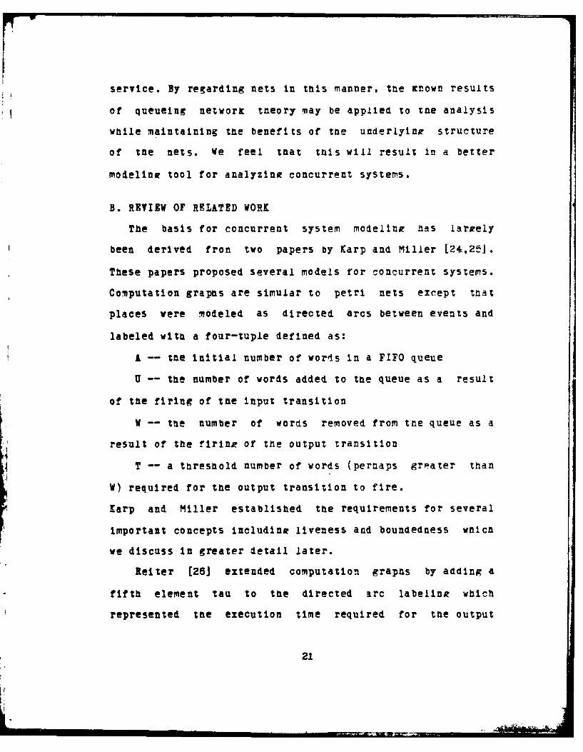
Computation graphs are simular to petri nets except that

places vere modeled as directed arcs between events and

labeled with a four-tuple defined as:

A -- the initial number of words in a FIFO queue

U -- the number of words added to the queue as a result

of the firing of the input transition

W -- the number of words removed from the queue as a

result of the firinA, of the output transition

T -- a threshold number of words (perhaps greater than

W) required for the output transition to fire.

Karp and Miller established the requirements for several

important concepts includine liveness and boundedness wnicn

we discuss in greater detail later.

Reiter [26J extended computation graphs by adding a

fifth element tau to the directed arc labelink which

represented the execution time required for the output

21

Ia

transition to process the V data words when firing. Reiter

then determined a metnod for finding possible sequences of

firings of transitions. For cyclic graphs, le found a lower

bound for tne cycle period of the graph. Computation graphs

have been used in the performance analysis of data flow

processors 2'?J.

The second paper by Karp and Miller [25J investigated

parallel program schemata ana vector addition systems. A

parallel program schema modeled parallelism In programs by

establishing computation states and rules for state

transitions. The concept of FOR[ and JOIN vnich nave been

applied to data flow and other MIMD architectures was

developed to express the creation of concurrent processes

from a sequential process, and the combination of concurrent

processes Into a sequential process. The equivalence of

petri nets, computation graphs, and parallel program

schemata was shown by Miller (28J.

Most of the research on petri nets in tne Unitet States

has been conducted at MIT. Commoner and Holt (li,12J studied

a deterministic subclass of petri nets known as marked

graphs and proved several theorems regarding their system

state spaces. A more general subclass of deterministic nets,

persistent nets, was studied by Landweber and Robertson [13]

who proved that the theorems recarding marked graphs were

applicable to this class. A final deterministic subclass

referred to as state machine decomposable was Investigated

22

LIWl

by Ramchandani. In addition, Ramchanlanl analyzed this

subclass with deterministic transition firint times to

derive expressions for the minimum net cycle period in a

manner analogous to tnat Reiter used for computation graphs.

Other classes of petri nets have been defined which

Improve the tractability of the problem of finding solutions

to performance measures while retainine characteristics

which are desired in the modeled systems. In particular,

live, bounled, conservative, and consistent nets nave

received the most attention. The properties of these classes

will be examined In detail in the next section.

Our vork extends this previous wort by focusine on the

broader class of nondeterministic, consistent petri nets

which appears to be the most general class for which

solutions to performance questions may be found. While

nondeterminism increases the difficulty of dealine with

petri nets analytically, much of the previous wort on petri

net structure remains pertinent to tnis class.

Nondeterminism allows the net to represent different types

of data, for example, by regarding the data type or

transition firing time as a random variable. To analyze the

performance of nondeterministic petri nets, we consider tnem

as analors to queueino netvorE models. The basis for

analysis of these models is the classic work of Jackson (29]

for tne case of open systems, and Gordon and Newell [3@1 for

closed systems. Both of these models relied upon poisson

23

arrival processes, first come, first serve (FCFS) queueing

discipline, and exponential service departure processes to

ensure that the Markov property was met and allowed the

system state probabilities to be expressed as the product of

the marginal state probabilities. This quality Is known as

the product form solution and is required for

computationally efficient solutions. Most of the recent work

In queuing network theory has attempted to find product form

solutions for more general systems. Jackson [311 considered

systems where tne arrival rates and service rates were

functions of the queue lengths (states) at the various

nodes. Baskett et al. (32] extended this to open and closed

networks where customers were of different classes and the

queueing discipline was FCFS, no queueing, and last come,

first serve witn preemptive resume (LCFS-PR). All tnese

cases were shown to have product form solutions. In

addition, they showed that a condition known as local

balance was a necessary condition for product form

solutions.

Chandy et al. (331 considered the question of local

balance in more detail and developed the more general notion

of station balance which was also shown to be necessary and

sufficient for product form solutions if non-exponential

differentiable service distributions were used. In addition

they proved that arbitrary service distributions satisfied

station balance if processor sharing (PS) or LCFS-FR

24

disciplines were used. In the case of exponential service

tiine distributions for all service classes, tney showed that

FCFS and priority disciplines resulted In station balance

beinR met. This result has been extended to any work

conserving discipline.

In summary, it has been shown that product form

solutions exist for queueing networks witn tne following

properties:

1. For exponential service, any work conserving queueing

discipline may be used.

2. For PS and LCFS-PR disciplines, any differentiable

service distribution may be used.

3. The solutions do not depend on the routing used for

the customers.

C. OUTLINE OF SUCCEEDING SECTIONS

In Section II, we present the formal definitions of

petri nets and derive several useful properties. The state

space -- the set of system states the net may occupy -- is

determined by constructing the reachability set of the petri

net. The conditions under which the state space Is finite

and recurrent are then considered. It is shown that nets

with certain structural characteristics give rise to these

restricted state spaces. In particular, the classes of

marked graphs, state machines, and consistent nets are

considered because of their relation to realizable systems.

25

In Section III we turn to nets with timed events. The

case of deterministic routine and transition time Is first

considered. Next, the (probabilistic) class of state

machines with nondeterministic routine and exponential

transition times Is examined. It is shown that for the class

of state machine decomposable nets it is possible to

transform the net into a stochastic equivalent net which is

analogous to a closed queueing network. For this class of

nets a product form solution for the state probabilities is

derived.

Next, petri nets which allow external sinks and sources

are defined. Again, it is snown that the stochastic

equivalent nets may be analyzed as queueine networks; in

this case an open system.

Finally, the class of consistent petri nets with

exponential firing times is considered and it Is shown that

product form does not exist for tlis class of nets.

26

II. PETRI NET THEORY

In this section the relevant petri net theory Is

presented. Much of the wort follows tnat of Commoner and

Holt (11], Kraft and Miller [25], and Ramctandani [EJ. Tte

notation used Is primarily tnat of Peterson (23J.

The petri net was defined informally in the precedine

section as a means for representing related events and tneir

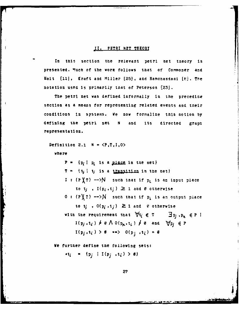
conditions in systems. We now formalize this notion by

defining the petri net N and Its directed graph

representation.

Definition 2.1 N = <P,T,I,O>

where

P- {pjj PL is a R in the neti

T = I1 ; t is a jr.Asition in the netj

I : (PXT) -->N sucn tnat If pL is an Input place

to tj , I(pj,tJ) . 1 and 0 otherwise

o : (PXT) -- >N such that if pi is an output place

to tj , O(pi ,tj) Z. 1 and e otherwise

wit the requirement that Vti ( T 3pi ,P, E P I

I(pi ,t i ) A e A O(p,,,tL) / o and Vj E P

I(pj,ti) > 0 => O(p ,t L) =0

We further define tne following sets:

% = {pj I I(pj ,t) > 01

27

S

ts. (p1 1 O(pj ,t) >1 where t ET APi'E P

and likewise:

0 = {t I O t(pj > 01

ptt I(pj ,t) > O1 where t4 E T A Pi E P

These sets are referred to as the input and output sets,

respectively. Note that the definitions of tne functions I

and 0 require that:

Vtt E To etz A~ Atie (P A oti U tie -- (

The set of places represents the conditions in our informal

model, and the set of transitions represents the events. The

input and output functions specify the preconditions for an

event to occur and tne results af the event occurrence.,

Correspondine to each petri net we define a bipartite,

directed grapn as follows:

VPZP" E P draw a circle representine a place

Vt, t, E T draw a vertical bar representing a transition

Vtz ,p. if pj E t4 draw a directed arc from pj to tj

Vti ,pj if pjEti* draw a directed arc from tj to p.

We will use the notions of petri net and petri net graph

interchangibly (since they are equivalent).

Example 1.

Consider the following petri net N = <P,T,I,O> with

P { P,' P ' P,, p4 9 Piro P, P

let n - and m = ITr . Then I and 0 may be

28

represented oy tnen X n Incidence matrices:

1 10 0C 000 0

00000 1 100000100 0100000a00 0010000001 0001 0

waere CT i,j - I(pi,tj)

and CO ,j - O(p i t j )

The corresponding petri net graph is shown in Figure 2.1.

If we associate with each place In a petri net N a

non-negative integer marking function j.,L we have the

following definition of a marked petri net M:

Definition 2.2 A marked betri net M = <P,T,I,O, >

wnere P,T,1,O are defined as before and

P ->N

Each function dLK defines a maring of the net. In graph

notation the petri net wraph is extended to a marked petri

net graph by adding tokens to places as follows:

VP" E P, if p-x(Pi) = n then place n tokens (dots) on

place p .

Figure 2.2 snows a possible marking for the petri net of

Example 1. Clearly a (countably) infinite number of possible

markings exist for any petri net. This marking represents

the (possibly multiple) holdinws of conditions at

29

I 7

T3

-t3

Figure 2.1. Petri net graph

30

T7

*1.

Tigure 2rCPernegrp

sove instant of execution and may be viewed as a description

of the state of the net.

Definition 2.3 & transition t Is enabled 1ff

VIpj pj E Oti -. > PL(pj) --> I(pi tz)

For each marking 4 we can define the enabling set SK as

follows:

Definition 2.4 The enablinR set S,,_ T = its t is

enabled by rarrina Lx.

In our graph notation, a transition is enabled if each arc

directed into the transition has a token in its originating

place. Referring to Figure 2.2, It will be seen that t,, tp,

and t4 are enabled and tnerefore ;, = {t , %Zt4 }.

Transition t3 is not enabled since there is no token in

place p. corresponding to the arc pV -- > t3 .

An enabled transition may fire to create a new markine.

That is, we define a function:

Definition 2.5 A firing runction for a marked net M is

"J. X S -- > L such that F(ji4pj),t-) = (pi) -

I(pi'ti) + O(pj. %) . Pt. .,

where pmeP A tcs.

F is defined for all markings for which the set Sp. is

non-empty. Continuing with the vector notation introduced

earlier for the functions I and 0, we may denote each

32

msrkin FLeas an n-element vector UK where n = P and

UX(i) = J.11(P;) for I = 1,2,...,n . Then F may be expressed

as:

F(U'At) = - +q. + CO: where C.p and CoZ are the ith

columns of the input and output incidence matrices

respectively.

Definition 2.6 Marring Lj is directly reacnable fromLklf

(t4 ES) A F(.pLtt) .!Lj and is denoted as:

Returning to our earlier example, transition tg may be fired

(recall that %tne enabling set S = l,, t2 , %4 1 )- By

Inspection of Figure 2.2, we specify the vector for marting

21

1000

The resulting marring , =

2 1 0 11 1 0 01 0 0 1

U.,"g -U 0 ~ 0 - 0 + 1 =1

A4V+ o 0 0 +1 10 0 0 0

0 0 0 0

In graph notation, one toten is removed from each place

having an arc directed into the firing transition, and one

toten is added to each place faving an arc directed from the

33

T'S

IP

firine transition. The resultinw marzine is shown in Firure

2.3.

Next we consider sequences of transition firings. Assume

the following firings exist for some marked net M:

Then we denote

ti ti a46=4L I => .L2 or L>.

where tae firing sequence Cris some sequence of transition

firings (;; ,t2 ,t,)"

Definition 2.7 Marring Is reachable from markinggi Iff

where .-

If we form the reflexive, transitive closure of the

transition firing relation we nave tne following definition:

Definition 2.8 "iven a marked net M, the reacfability set

Q(M) is defined inductively as:

basis: 41. e QInduction: .L, e Q A 3t E T 114, JLinL I.uEQ0

We are interested in determinine the elements of the set

0(). To do so, we must first formalize the previously

introduced vector notation as a vector addition system.

35

A. VECTOR ADDITION SYSTEMS

The concept of vector addition systems was first

explored by Carp and Miller [25J. This section is largely

derived from their wort.

A vector addition system is defined as a pair V = (d,W)

where d is an r-dimensional vector with IiEN and W is a

finite set of r-dimensional vectors w,, w., ..., wft with

wj(i)EI. The reacnability set R(V) for a vector addition

system is the set of vectors composed by adding elements of

the set V to d. That Is

R(Y) a x I x = d + (w, + w. + ... + w, A x() .In addition, the following terminology is used:

The relation :S is defined as

x y <=> for i = 1,2,...,r x(i) y(i)

The symbol W is defined such that if n is any Intemer,

( >J n and n+ =W.

The reachability set R(T) can be determined by constructine

tne corresponding reacnability tree T(V). Nodes in the tree

consist of r-dimensional vectors x,y,z,... with

x(w)E N Ufl, for i = 1,2,...,r . The relation < is defined

as x.( y <=> a directed path exists from x to y in T(V). Let

d be the root of the tree. Descendants are constructed

recursively as follows:

1. If x . y and x = y, y is a leaf node.

2. Otnerwise, construct successor nodes to y with

vectors y + we, y + w2 , ... , y + wf where for i =

36

S1,2,...,r y(i) + wj(i) _. In addition, if tnere exists

a node z such that z. y and z-.y + wj and z(j) <

y(j) + wi(j) for some J, tnen y(j) + wz(j) =Gj.

To illustrate the construction of this tree consider the

following example from (251 :

Example 2.

Let V = (d,W) where

d- { [-1,,0,0,1 , [-1,0,0,1,0] ,

I s1,-,0, ] , [e,,0,-192] , [0,0,9,1,-i]

The resulting reacnability tree is stown In Figure 2.4.

The followine theorems from (251 allow us to answer

decidability questions about vector addition systems by

Inspecting the reacnability tree.

Theorem 2.1

Vx 3y 11y E R(v) A (x .5Y) <=> z 1z r:T(V) A (x .5z)

The proof, while straicht foward, is rather lenwthy and so

is not Included aere, but may be found In [25].

Theorem 2.2 For any vector addition system V, T(V) is

finite.

We first show the follovine two lemmas:

37

III I IIi-I "" ' • - - ". . . . "

°-

00

0 07 C7a :3 0

00 0-o 3 0,o

a ao00

0 0

00

C0 0

Figure 2.4. Reachability tree for Example 2.

38

Lemma 2.2.1

Let p, ,ptps, -.. ,P., -- " be an infinite sequence of

elements of (N U4J) • Then there exists an Infinite

subsequence P% ,P,P,"- ,Pat ... such that

P.M. P4 ...ft . ....PI --

Proof. Construct an Infinite subsequence by selecting

elements with first entries nondecreasing. From this

sequence, construct an Infinite subsequence with second

entries nondecreasing, and so on.

Lemma 2.2.2 (Kdnig Infinity Lemma) Let T be a tree such

tnat each vertex has a finite number of successors and

there exists no Infinite directed path from the root.

Then T is finite.

Proof. Since each vertex nas a finite number of

successors, let n be the maximum number of successors

for any nole. Then there are at most n paths of lengtn 1

from the root, and if p is some node in the tree, there

are at most n paths of length 1 in the subtree having p

as its root. Since no infinite patn exists by

assumption, let m be the maximum path length. Then the

maximum number of nodes Is n and T Is finite.

Proof of theorem 2.2.

Assume tnere exists an Infinite directed path from the

root of T(V) with node sequence P,,PPj,.*.',Pn,...

39

Then by lemma 2.2.1, tnere exists a subsequence

p, p , .,p, ...,p .VI pv!P ... , paa. . . By

definition, if p,= p. then pt is a leaf node and

therefore the inequality is strict and

P.6 <P4 <P,**<Pa < ... . Again by definition, since

P4 <Ps, p4 must have one more entry equal toc Jthan p,.

Since tne number of entries is finite, this is

impossible and therefore no such Infinite directed path

exists. By lemma 2.2.2, T(V) is finite.

Using these theorems, It is possible to prove tne following

decidability theorems about the reachability set R(V):

Theorem 2.3 Given some finite nEN ,

Vx % f R(V) A (x(i)-O a) is decidable.

Proof. Construct T(V). By tneorem 2.2 T(V) Is finite.

Therefore Vy y ET(V) A(y(i) n) is decidable. 2y theorem

2.1 then, the question is decidable for R(V).

Theorem 2.4 Given some subset of tae entries for tne

r- dimensional vector addition system GS; {1,2,...rj,

Vxxe.N "3T y eit( V ) A(VI I f-e)y(i) 'z(i) Is decidable.

Proof. By tee definition of T(T), this property holds iff

there exists a leaf node z such that Vi iEe z(i) =Cj

40

Theorem 2.5 %iven a vector addition system R(V), It is

decidable wnether R(V) is finite.

This result follows directly from theorem 2.4.

Theorem 2.6 Given two vector addition systems V and V',

R(V)_C_ R(v") is undecidable.

Rabin's proof for this result appears in Baker 134J.

It should be noted that the general reacnability problem

i.e., given xENr is x ER(V), is not determined by the

reachability tree. However, an algorithm for solving the

reachability problem has been found [35]. Therefore, the

reachability problem is decidable (although the

computational complexity is not known).

This completes our study of vector addition systems. We

next demonstrate the correspondence between vector addition

systems and marked petri nets. Let M = (P,T,I,O,> be an

arbitrary marked petri net. The corresponding vector

addition system V(d,W) may then be constructed in the

following manner:

let the dimension r = IPI

let d =f4L. wverel.. is an initial marring for M

let W - tw., t E Ttp;E P w,((J) = O(p1 ,t.) - I(p;,t i)

Note that IjV - IT I and that elements of V reflect the net

change in marking resulting from the firink of a transition

41

In M. This leads to the following tneorem relating the

reachability sets of M and 7:

Theorem 2.? 0(M) = R(V)

Proof. 1). Q(M).-R(y). Let x ER(M). Then

By definition of w

l(pt 6 ) = w, and substitutine for t,, tg, t3 , ...

t,, in the firing sequence JL w, * w+ * ...w, - X

Since IL.= d by definition, zE R(V)

ii). Q(M)-R(V). Let x ER(V). Then

x - d + w, + w + ... w . By the same reasoning as case

z, u -/ *->... .I

Using theorem 2.? and the results for vector addition

systems we state the following:

Theorem 2.8 Irven a marked petri net M with initial

martingp., it is lecidable if the reachability set Q(M)

is finite.

Theorem 2.9 Given a marked petri net M with initial

marking IL, , it Is decidable if there exists jEEJ, such

that for all elements of the reachability set Q(M),

each entryJ.() .

Definition 2.9 A marked petri net M is k-bounded iff

42

H - 0 O H CD)-4 00 H 0-iO -1 0 HO r4

0 CD0 O=7 H c 0 H 0 0 0 0D 00r-

0 D C>O 00O H OHH H 0 0 CDa a a7 a' a= H^ a 7 a= a a -1 a ^ a a= aa

C' CJcjCJrj CD C D C\CJCJ H\ C0 C

0 0 00 CD 00H 0 CDi

C) OHHO 0 H 0- C O C 0

17VV7 r-4C7JV) fDV0 ) 0C0 H 0- 0 0 0

a a a a0 -l 0- r0-i 0 -=

a a aa a a a aD

Fiur 2.5. Hecab t tree Ho Hxample0

Definition 2.10 A marked petri net M Is safe itff It is

k-bounded with X a 1 .

We complete tals section by once again considering Example

1. Define tne corresponding vector addition system:

1 = (d,W) with d = [2,1,1,0,0,0,9j as Indicated by

Fiture 2.2.v = { [-1,s,e,i,,e,osJ , (-i,-i,o,i,1,o,oJ,

V,

[0,e,1,0,s,e,-1| }

Next, construct the correspondine reachability tree T(V).

The tree is shown in Figure 2.5. By Inspection, the

reachability set R(V) is determined to be:

{ [2,i,1,o,o,o,o] , (1,1,1,1,0,0,0] , [i,e,i,1.,i,o,oj,

[2,1,e,0,0,0,1] ,[0,1,1.2,0,0,0] [0,0,1,2,1,0,0]

[o~le,2o~o1] [o,s,e,2,1,0,iJ , (e,1,0,2,0,1,e],

[o,o,o,2,1,1,o] I

This (finite) set is also Q(M) and therefore M is t-bounded

with k = 2.

B. SUBCLASSES OF MARIED PETRI NETS

The nets Investigated in the preceding parts of this

section are more properly referred to as generalized petri

nets. Analysis of generalized nets has proved to be somewhat

intractable. As a result, several properties of petri nets

have been studied which define subclasses of the generalized

44

lag~

Figure 2.6 Nondetermintstic net -- botI U and t2 are enabled.

45

'Ago

nets. These restrictions appear to be Justified in that many

(if not most) actual systems may be modeled by the

restricted nets.

Definition 2.11 A transition t T is I "v for marking 14

i ff

where i is the enabling set forP.L

If a transition Is live, a firing sequence may always be

found which will allow it to be fired indefinitely often.

Definition 2.12 A marked petri net M is live iff

Vt tET > t Is live for markinep,

In systems, liveness is often associated with the problem of

deadlock. Hack (36] has shown that liveness is equivalent to

the reachability problem; therefore, It Is decidable.

Definition 2.13 A place peE P is conflict free 1ff

Y Lktj . ...a a* t,, E Pjo A t;sn=3tj 1 At;Es,

Yor any marking, a conflict free place may not enable more

than one transition. In Fieure 2.6, place p, is not conflict

free since both t, and t2 are enabled.

Definition 2.14 A petri net M is conflict free iff

V p EP m-) p is conflict free.

46

A stronrer statement concernine places is the follovine:

Definition 2.15 A place p is decision free iff

j.P4 = IPLi 1

Definition 2.15 A marked petri net M is a marked graDn iff

p p JP -=> p is decision free.

A final property of petri nets may be defined:

Definition 2.17 A markine . is iersfsten, ff

Vt ES A (,IJ=>I,,) -=> tE S, V to

A persistent marking Is one in which an enabled transition

remains enabled until it is fired.

Definition 2.18 A petri net M is persistent iff

Vt t ET ==> t is persistent forL.

The question of persistence Is important In the analysis of

petri nets ani tterefore we present a decidability theorem

for these nets:

Theorem 2.10 Given a K-bounded, marked petri net M, it is

decidable whether M is persistent.

Proof. Since M is k-bounded, its reachability set O(M) is

finite. For each j.. E Q construct the enabling set Sk.t,#

For each tj E Sft determine S,, wnere = .L l, , . If Sk,

,-SK - {t ij , M is persistent.

47

Note that all conflict free nets (and therefore all marted

graphs) are persistent. We next consider some aspects of the

petri net classes naving these properties.

1. Marked Graphs

Marted graphs nave been extensively studied by

Commoner and Holt, among others [11,12]. Here we present

some pertinent results of their wort.

Recall from craph theory the following three

definitions:

Definition 2.19 Let D - <A,R> be a dieraph with nodes a

and b. A directed patn from a to b is a finite sequence

of nodes P = (co,c, .... c.) such that c. - a, c' = b,

and for all c. with0 :5Si<-n cjRc., . If a = b, P is a

directed circuit.

Definition 2.20 A dieraph D = <A,R> Is strongly connected

if for every two nodes a,bE&, there is a directed path

from a to b and b to a. If there is an undirected path

from a to b, D is connected.

Definition 2.21 A component of a digrapa D is a connected

subdigraph of D which is not a proper subdieraph of any

connected subdigrapa of D.

The constraint on the input and output transitions to a

place mates it possible to replace every place with a single

directed arc between its input and output transitions. In

V 48

this way the petri net reduces to a digraph simplifying

analysis. The marked graph may then be more simply defined

as:

Definition 2.22 A marked graDn M' = iT',E',Z.> is a

three-tuple where

T' =T

E" : TXT -- > {0,i1

if 3p O(p,t ) 1

where Z(t ,;) -A I(p,t ) = 1

otherwise

: " ->Nvnere

(e) = p

where eqEE A*P.p - {t iA P. - it]}

(Here we have synonymously defined the edge set

V' - {ej} where the edge directed from node 1 to

node j eqEZ' 1ff 2'(ti,tj) = 1

Additionally define tne token count N as:

Definition 2.23 The token count of a wraph is a function

N : P -- >N where

if P -.. then N(P) -Z}.(e ) for eEP

Figure 2.7 snows tne graphical representation of a marked

graph where the number of tokens on an edge e~j corresponds

to g'(e,,). The following theorems and proofs appeared in

49

Flure 2.7 Marked graph. Note that tokens are placed on the arcs.

5.

Theorem 2.11 A marking "L' is live iff the token count

N > 0 for every directed circuit In M.

Proof. 1). Assume " Is live and N(B) = 0 for some

directed circuit B and ezj is an elre in that circuit.

By definition, a sequence (7exists which enables t-.

After firing p'(e~j ) = 1 and therefore N(B) = 1 in

contradiction vith the assumption.

ii). Assume N(B) > 0 and tj is a node in directed

circuit B. If t i is enabled, tj is live. Otnervise let

t " be a node In B such that eii is in B. If ti is

enabled, fire It resulting in ti being enabled. If not,

continue to backtrack. Since the path lenath of B must

be finite in the directed circuit beginning and ending

with ti, this procedure must halt and therefore tj is

live.

This leads immediately to a corollary:

Corollary 2.11.1 A marking which is live remains live

after firing.

Theorem 2.12 A live marking Is safe iff every edge In the

graph Is In a directed circuit with token count

N(P) a I.

Proof. Clearly, the token count of any directed circuit is

constant. If N(P) 1 then, the edees of the directed

51

circuit must oe safe. If N(P) L > 1 , by the same

process as in tneorem 2.11 transitions in the circuit

may be fired until k tokens appear on tne same edge.

Theorem 2.13 For every finite, strongly connected grapn G

there exists a live and safe marking for the

corresponding marred grapn M'.

Proof. By definition, each edre in G must lie in a

directed circuit. Since G is finite, a finite number of

directed circuits exist. Therefore construct j./ by

placing one token arbitrarily on each directed circuit.

The conditions of tneaorems 2.11 and 2.12 are met and M'

Is live and safe.

2. State Macnine Decomposable Nets.

This class of petri nets has been studied by

Raicnandani []. A state macnine is defined as:

Definition 2.24 A marked petri net M is a state macnine

1ff

Vt t T A [I(p ,) > 0A [I(pjt) > 0J ==> p . = piVt tET A [O(p.,t) > 01 A [O(pj,t) > 01 =0-> p,. pi

That is, Vt I .It-I 1

This restriction results in nets which are functional

equivalents of finite state machines, hence tue name state

52

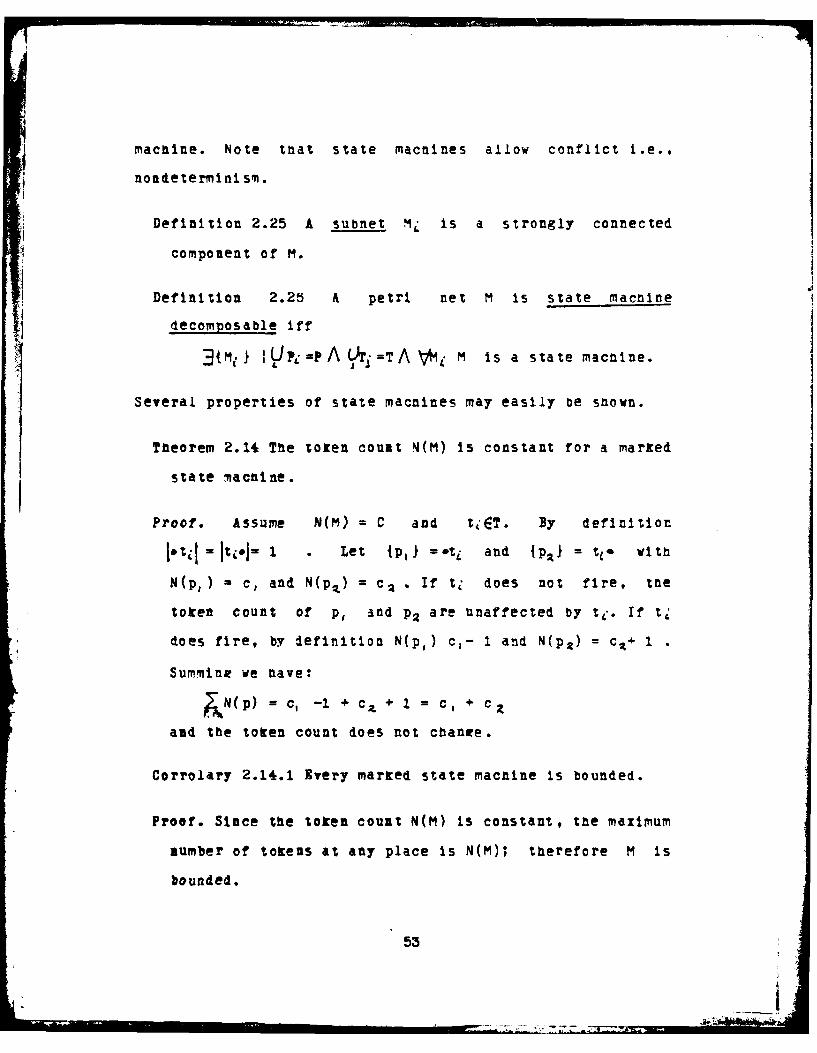
machine. Note that state macnines allow conflict i.e.,

nondeterminism.

Definition 2.25 A subnet M4 is a strongly connected

component of M.

Definition 2.25 A petri net M is state macninedecomposable iff

3tm,- 1 iP ALIT -=T A VM e M is a state macnine.

Several properties of state machines may easily be shown.

Theorem 2.11 The token count N(M) is constant for a marked

state macnine.

Proof. Assume N(M) = C and tET. By definition

I0tilI jtil-j 1 . Let Ipt,1 =.tj and {paj = tj- with

N(p,) = c, and N(p.) = c2 . If t does not fire, tne

token count of p, and p. are unaffected by te. If t

does fire, by definition N(p,) c,- 1 and N(p.) = c,+ 1

SumminR we have:

.1, N(p) = c-1 + X + 1 = c +C

and the token count does not chance.

Corrolary 2.14.1 Every marked state machine is bounded.

Proof. Since the token count N(M) Is constant, the maximum

number of tokens at any place is N(M); therefore M Is

bounded.

53

3. Consistent Petri Nets.

An additional class of petri nets are those for

which there exist consistent current assignments.

Definition 2.27 A petri net M Is consistent iff there

exists a function cp: T --> I such that

2. VpEP x '(pet4) 2 =x o(petj)

where in the summation n =I

The function 4 Is analogous to an electromagnetic flux and

the (pis are referred to as the currents associated with

transitions te. Note that part 2 of the definition Is an

expression of Kirkhoff's Law. Part 2 requires solving the

following set of linear equations:

CZ, .......... C % , C 0 . .............. C0 4 '

CC ...... ... ... COd (PA, . o

where Cr and C0 are the Incidence matrices for M.

If a non-zero solution exists, M is consistent.

Example 3. Consider the net In Figure 2.0.

10600Construct Cr 0 0 0 1 0 CO 0 1 0 0 00 00 01 0 010 0

1 0 0 0 00 11

5f T

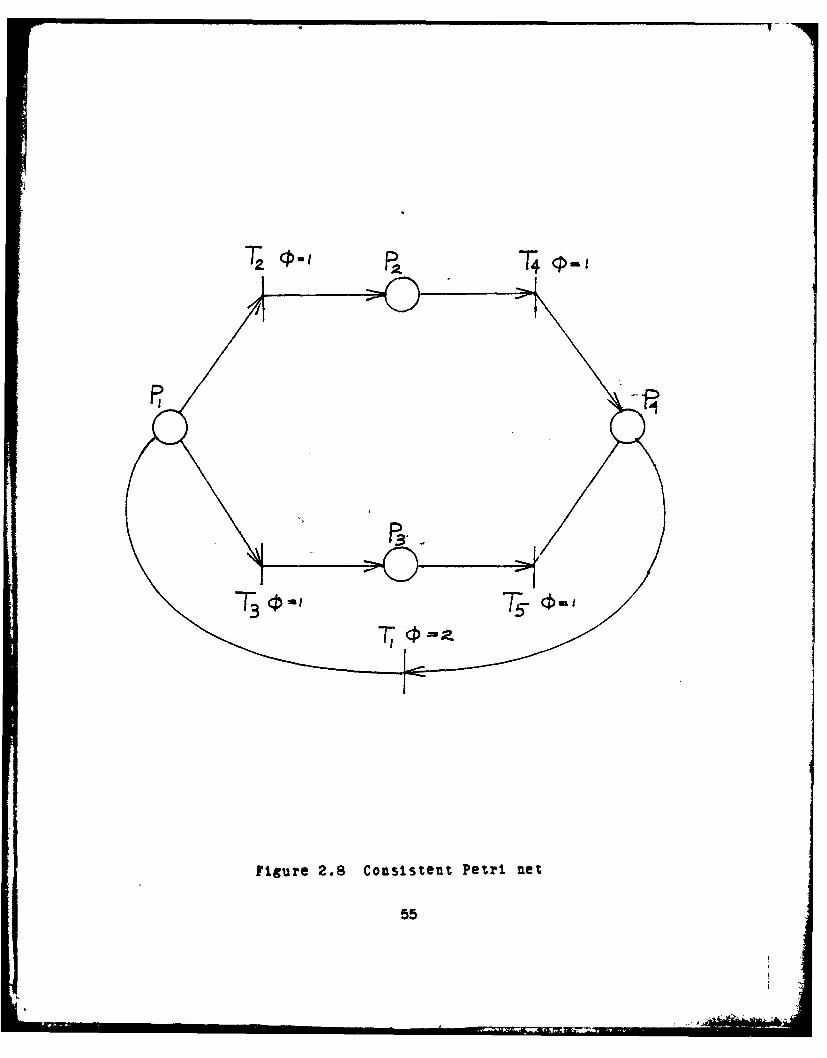
Figure 2.8 Consistent Petri net

55

0 1 1 00

obe * p

Therefore M is consistent.

The siwnificance of consistency is that a consistent system

will cycle -- given an initial mar~1ngg., there exists a

firing sequence suchl tnat1 Lo - &n inconsistent system

will either consume tokens and halt or produce tokens and

become unbounded. These results are summarized in two

theorems by Ramchandani [8].

Theorem 2.15 A petri net M is consistent if?

3. "such that .,C=/. is a cycle.

Proof. 1). Let ,, .. be the consistent currents of

the transitions or M. Le to~ , = czP+ p+cp=c vnere

.c • . correspond to tL" .. .AEp . . Then letCI XC10

c 7= { 1 ,t...1 where the multiplicity of t, inO'is

equal to its current giving J,, =>pi . Since the sum of

tne currents into and out of a place is 0,

gLoPC) -L-j(pi) and .L mp. . Therefore a-is a cycle.

ii). Let 4.J>=L.be a cycle. Then .L(po.) =>4.(p;) . Let

be the multiplicity of transitions

to ,t 2 .. 9-t, E*P, and 1, be the multiplicity of

transitions t 'tag...9t Ep. . i =Tli . Then let

:ti) t " if t,.op, andcL:ti) = i i if t 1 EP.e . This Is

a consistent current assignment and therefore M is

consistent.

Theorem 2.16 A petri net M with a live, bounded markine

is consistent.

Proof. Since M Is bounded, its reachability oraph Q(M) is

finite. Since M Is live, tnere exists a strongly

connected subzraph which contains j. Therefore, tnere

exists a directed circuit In the subgraph firinw all

transitions. This is a cycle and therefore M is

consistent.

We conclude our description of petri net subclasses by

considerinw the hierarchical relationsaips between classes.

In the sections on marked graphs and state machines, it has

been shown teat both are contained within the class of

bounded petri nets. It is easy to show that the containment

5?

Ficure 2.9 Bounded Petri net

58

Figure 2.10 Unboundedt non-live, consistent net

59

figure 2.1.1 Petri. net hierarchy

is proper. Figure 2.9 snows a net wnicn is bounded but

neither a marked graph nor a state macnine. The intersection

of the class of marred grapns and state macnines are a

derenerate class ye call sequential processes. Theorem 2.16

showed that all live, bounded marked nets are consistent.

Once again, the containment is proper -- Figure 2.10 Is an

example of an unbounded non-live net which is consistent.

Finally note tnat all persistent or conflict free nets are

deterministic and therefore may be reduced to decision free

nets I.e., marred graphs. These relationsnips are summarized

in Ficure 2.11.

61

III. STOCHASTIC PETRI NETS

To this point we have analyzed petri nets on the basis

of their structural characteristics. To utilize petri nets

for computine performance measures, it is necessary to

Introduce tte concepts of time and nondeterminism to tie

basic model. We turn first to the question of modeling time

In petri nets.

A. TIMED EVENTS IN PETRI NETS

An important concept in Section II was the marting, or

system state, of tne net. The marking gives an instantaneous

description of the token content of each place in the net.

The marting was changed as a result of tne firing of a

transition. We defined a firine sequence as an allowable

ordering of transition firings in accordance with the rules

for enabline transitions. By controlliut the dynamics of the

transition firing process, it is possible to analyze the

changes in system state as a function of time.

Several authors nave addressed the question of addine

timing considerations to petri nets. Two different

interpretations have resulted from this wort. Sifatis (37J

has proposed that once enabled, transitions fire

instantaneously. A delay is then introduced before tokens

are available at the output places for possible enablines cf

other transitions. An alternattve viev is that taken by

Ramchandani [9 and Zuberet [38]. In their models, once

62

enabled, transitions fire after a delay called the firing

time. After the firing time is completed, the net changes

state by moving the appropriate tokens. These two

Interpretations appear to be equivalent. We choose to use

the latter interpretation to conform to the usual notion of

a queueing service center.

We first consider the case where transition firines

occur at discrete time epocls ,f9 V...,,... where'r., is

the instant of the nts firing.

Definition 3.1 The system state of a marked petri net M Is

a function:

U:T -> gLvhereT" t' ,'..., ... 4U(f*) =Lo I

and U(-r,) = A> i !u(-r.) it

U Is a step function with discontinuities at those instants

of time in which the system changes state.

Definition 3.2 The firing time I of a petri net is a

function:

11: T-->e +

where tt E T I(ti) - x a

By t is definition, zi is tne time required for a firing of

the transition tz.

63

I l III I I I I( Fil Il .. . ii l . . . ,

By specifying the firing time function X, it is possible

to describe 3(t";). In this section we consider the ease where

the transition firing times xC are constant for all

transitions. This restriction makes it possible to describe

a total ordering of transition firings for persistent nets.

In the case of allowed conflict between transitions, it Is

necessary to impose a priority scheme on transition firinrs

to resolve the conflict (that is, to make the firing

deterministic). This ordering amounts to a restriction on

the firing sequences whicfh are allowed. Those sequences "

for which the ordering holds are termined feasible firing

schedules. Ramchandani has shown that for timed marked

graphs and live, safe, and persistent petri nets a periodic

feasible firine schedule exists. He additionally derived an

upper bound on the computation rate (cycle period) for state

machine decomposable nets. The bound is given by:

p max = minpP 2 9P,,J

where p n is the cycle time for each circuit in the

corresponding net and is given by:

N(Ci)

where N(Ci) is tae token count for circuit C,9 Xj is the

sum of the firine times for the transitions in Cj, and ckLis

the current associated with that circuit in a minimal

current assirnment. Rtamcnandant also argues that this

formula can serve as a first order approximation where the

64

"= = 1=

mean firine tlmes-i are substituted for the deterministic

firing time x in the formula. A slightly different

derivation of tte same result was made by Ramamoortay and Ho

(39].

B. MARKO! ANALYSIS OF PETRI NETS

Research into tae behavior of timed petri nets to date

has concentratel on deterministic nets with constant firing

times. As noted in Section I, this approach fails to account

for the randomness and uncertainty wvficn characterize actual

systems. We propose that nondeterminism be modeled

probabilistically In zne net. Our method differs from

previous wori by emphasizing the stochastic nature of the

system state (marting). In this way, it is possible to apply

the tnown methods of queueine theory to analyze tne

probabilistic properties of these nets which we call

stochastic petri nets. We introduce in this section two

sources of nondeterminism which will be modeled by the

stochastic petri nets -- random transition firing times and

the probabilistic firing of simultaneously enabled

transitions.

We first show that if the firing time x for each

transten is considered to be a random variable rather than

content of the net as a stocnastic process.

65

Definition 3.3 The firint time 14 Is an Independent,

Identically distributed, random variable such that

Vti E T x~j is the firing time for the att firing of

transition tz .

The requirement tnat IL Is Independent and Identically

distributed is necessary for our derivation of a Marrov

cnain representation for the net state space. In the case of

computer networks, Kleinrock (4o] has investigated this

requirement which he has named the message Independence

condition. This assumption Is somewhat artificial in that It

implies, for example, that the time required to process the

same message at two nodes is Independent. This difficulty

notvithstandine, results for an analysis of the ARPA net

stov some evidence for the validity of this assumption 4:11.

Applying the methods of probability taeory, the firing time

distribution may be defined as:

Definition 3.4 For all tiET, If i the firing time for

tit

SO(X) - P(X S x)

In the usual way we define the density function:

Definition 3.5 For all transitions ti .T, tie firing time

density function Is given by

si(x) = d/dz [S,'(x)] = p1i = x]

66

Likewise define the moments:

Definition 3.6 The ntft moment of the firinu time density

function is given by:

= fxns(x~dz

and In particular S[X J ="iC - 1/p.j is the mean firing

(service) time*.

These definitions make it possible to model systems by

applyinw the appropriate distributions to the firine time

function. It is clear tnat the feasible firing sequences Q

for a petri net are no lonrer deterministic. It is necessary

to consider tow tnis nondeterminism can occur in the net.

Referring to Figure 3.1(a), it can be seen tnat transitions

t and t4 are both enabled. itin random firne times, the

sequences t2 ,t4 and tj,t, are both possible. In this

instance the effect of the nondeterminism is unimportant to

overall system operation since the two processes are

Independent at this point. A more interesting situation is

depicted in Figure ;.1(b). The transitions ta, t, and

are in conflict. To analyze this type of nondeterlinism it

is necessary to specify the branching probabilities for each

of the possible paths. There are several possible ways this

may be accomplished. For example, each simultaneously

The mean service rate J. Is an unfortunate conflict innotation. Due to its lonR standinw use in the literature, wewill use tais notation pointing out its meaning whereconfusion might exist with the earlier definition ofmarkine.

67

!P

(a)

' (b)

Figure 3.1 Nondeterminism in petri nets. (a)Independent processes. (b) transitions with conflict.

68f

enabled transition may begin firing at once with the

transition which completes firing first causinp the marine

to change. Tne problem of determining which transitions are

simultaneously enabled is a sinnificant one. We can simplify

the problem by restricting our analysis to free choice

places.

Definition 3.7 A place p Is free choice Iff

pia = 1 V Vj ET tJEP(& tP>

A free choice place Is one which either has a unique output

transition or is the only Input place to each of Its output

transitions. This restriction ensures that a marking for p

will either enable all of Its output transitions

siiultaneously, or will enable none of them. With this

restriction, It is now possible to define the branching

probabilities for the output transitions of a free choice

place.

Definition 3.8 The branching probability for a free choice

place pi with pi* = {t 1,t 2 ,...,t} is

b~i. - P(tj will fire , are enabled)

such txat:

6 < bij * 1

and

bij - i where n

69

We make the assumption that these probabilities are

functions of the firing distributions for tne output

transitions only and in particular, that they are constant

and independent of the marking.

By allowing these sources of nondeterminism, the system

state U may be expressed as a stocnastic process.

Definition 3.9 Let U(1-), the system state of a petri net

M, be a random variable and a function of time vnere

U(1) [u, (1 ,u2 (-) 9...u,, (-r)] such that uj (-r) =. (pi).

U( ) is a discrete state, continuous time stochastic

process described by the probability distribution:

f,(u~ = p LU (1r) -;J., , U(-fj P2) =±,.u(-r) =I

U(i1 describes the manner in wvich tne system moves

between states in the reacnability set. It should be noted

that the distribution f.,(4:1n is equivalent to expressing

the probability that some feasible firing sequence (7 exists

such that Therefore, it is possible to extend tne

definition of liveness.

Definition 3.10 A transition t ET Is live for state U

iffVu g3 i 5. p(Or, >,e -->Baj j

LV icr 0ii A:O10=70

Theorem 3.1 For a live stochastic petri net M vith markiin

and initial marting LJ oEQ(M),

p(T) =L. > 0

Proof. Assume p(U(-r) =1-LU = 0. Then the probability that

a firine sequence 0- exists such that ,L=>1J. is zero In

contradiction with the assumptions of Definition 3.10

and therefore M cannot be live.

We are interested in determining the conditions for which U

Is a Markov chain, that is, when

p[U('rn. ) 1., U(1In ) - L.,U, {J'i. )=L.. ,.

,U('i -PL.] = pCU(,,., ) =,.,. I U(,r,) =/.,].

In addition, we are interested in determining the

stationary (time independent) state probabilities if they

exist. We first consider the case of state machine

decomposable petri nets.

C. CLOSED PETRI NET SISTEMS

To express tne system state transitions as a Markov

process it is first necessary to derive expressions for the

arrival and departure processes for tie places in the net.

This may be accomplished by considerine the net as a

collection of nodes, each of which has a well-defined

besavior, and in particular, for which tne arrival and

departure processes may be expressed analytically.

71

A node in a petri net Is defined as:

Definition 3.11 & node n in a petri net is a subset of the

set {PUTI such that

E T tEn <->

1VPj PE't <=p> pj En

AVt ,. tx EP <== t En

Theorem 3.2 Tne node set (nJ = n i , n2 t...,n.) is a

partitioniaz of a petri net M.

Proof. 1.) Uni =tPUTI. By definition, every transition t

is trivially an element of some node n4. Assume there

exists a place pj such that pj (n, n 29 ... ,niq). By the

definition of a petri net, pj has (at least) one input

transition ti. Since tL is an element of some node, by

Definition 3.11 pj Is an element of that node.

ii.) Vn n E [nJ na - n V n.f n6 =. Assume there

exists some transition tiEtn.fn nij. Let pi be an Input

place to t* and an element of n.. Tnen oy Definition

3.11 Pi is also an element of nb. Now let t be an

output transition to pj and an element of n a . Atain by

definition tr is also an element of nb and therefore

Likewise, assume there exists some place

pi E{n.lnb. By the same reasonine n,. nb. Therefore,

the set of nodes defines a partitioning of M. QED.

72

(a)

(b)

Ficure 3.2 Queueing nodes in petri nets. (a) partitioning of anarbitrary net. (b) single place/transition node.

73

Figure 3.2(a) snows the node partitioning of an

arbitrary petri net. Now consider the single

place/transition node n,. Figure 3.2(b) Is tnis node with an

arbitrary martinR. Since we have assumed that the transition

In this node is firing whenever enabled, we nave the

important result that this node is equivalent to a single

server queueing system.

The marking for p, which we have defined as the state

element u, includes the tokens being fired or waiting to

fire. Two features of this representation sneuld be noted.

First, all tokens are identical; no token classes exist.

Second, no queueing discipline is modeled In the system.

This places a restriction on the ability to derive analytic

solutions for the system.

To describe the operation of tne node, tiat is,

determine the local state probabilities PtU(fr) = u), it Is

necessary to characterize tne arrival and departure

processes. It Is well known that the exponential

distribution is tne only continuous distribution for which

the Marro property holds. In addition, It has been shown

(33] that arbitrary work conserving queueing disciplines

result in equilibrium product form state probability

solutions for exponential firings. Therefore we assume the

firing time distribution S(x) to be:

74

Definition 3.12 The firine time distribution for

transition t:. Is given by

Si (x) 1 - exp(-/.,x)

where the mean firing rate isj. .

The requirement that the queueing discipline be work

conserving means tnat no knowledge of the firing timne

requirements is used In selectint tokens for firinR. It is

clear from the Indeterminate nature of the tokens in petri

nets that this Is indeed the case and therefore we are

justified in asserting that the Markov property holds.

Finally, It Is necessary to determine the arrival

process for the node. In the case of closed networks (and

the petri nets ye have considered thus far), the arrivals

are made up of departures from other nodes in the net. It Is

assumed that upon completion of firing, the tokens

Imediately enter their associated output places. Therefore,

the arrival process may be characterized as:

Definition 3.13 The arrival rate L for a place p4 Is

given by:

where Ii is the arrival rate for node ni, bjL is the

branching probability tnat a departure from node nJ

arrives at node nL, and m is the rank of [n].

7541

Note tnat we nave not specified the arrival distribution

itself. It has been shown by Burge's theorem [42J and

several extensions (for example (31), tnat in many cases the

arrival process is asymptotically Poisson.

To summarize, we have made the following assumptions

concernine the petri net state transition process:

1. Firing times are independent.

2. Firine times are continuous and exponentially

distributed.

3. The queueine discipline Is work conserving.

4. Nondeterministlc transitions between nodes are

determined by constant branchinR probabilities.

5. There is no overhead in transition firings;

transitions fire whenever enabled.

In Section II we considered the class of state macnine

decomposable nets and state macnines. Figure 3.3 is an

example of such a net with its associated nodes.

Theorem 3.3 Each node in a state machine contains exactly

one place.

Proof. By definition, each transition has a single input

place. Trivially then, there must be at least one place

in each node. Without loss of generality, assume tnere

exists a node with two places p, and wDR with t p" By

implication, t#p. and therefore pi-t" in

76

contradiction with tne definition of a node. Therefore,

there is at most one place in each node. QED.

The next result follows immediately:

Corollary 3.3.1 The places in a state machine are

free-choice.

Since the places are free-choice, it is possible to

assign tne branching probabilities to the output

transitions. These transitions are not multiple servers;

rather, they represent the possibility for tokens whicn must

be handled differently. It is necessary therefore, to create

composite places to deal with this requirement. The

resulting net we call the stochastic equivalent petri net

(SIN).

Definition 3.14 The stochastic equivalent net for a petri

net M is constructed as follows:

For every place p in P, assign a set t-ff,,Tr,...,.Tf }

where n = p.1, Vt T ; (-rt) = I(pZ, t) , and if

0 O(PZO Juto(-rr , ) = { t herise

In the associated graph, each edge from a transition in opi

to the set t-,r.....,.!} Is joined by an arc and labeled

with tne appropriate branching probability.

77

FIaure 3.3 Partitioninn of a petri net Into a node set.

78

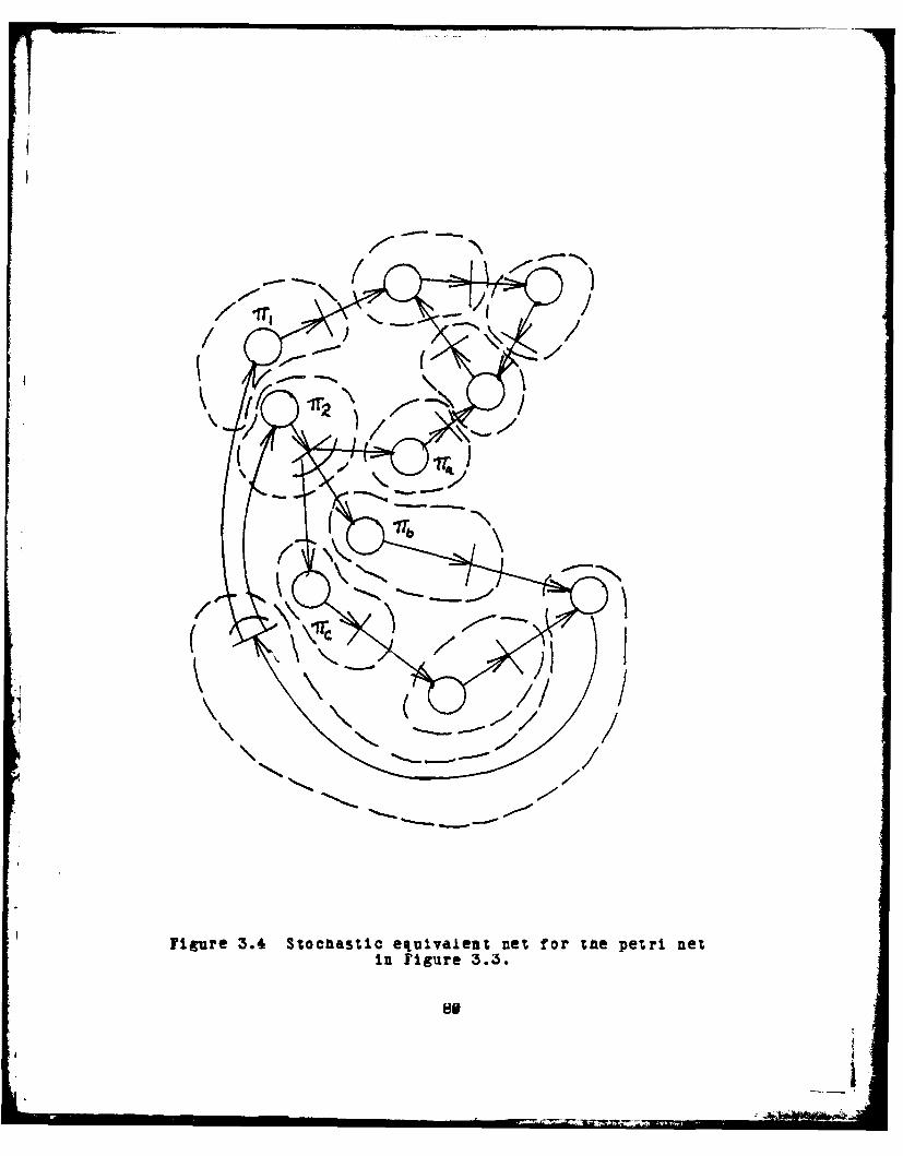
The SEN for the petri net in Figure 3.3 Is depicted in

Figure 3.4. Each node in tne SEN consists of a single place

and transition, with the branchine probabilities occurrine

at tae output from tne transitions. It Is clear from the

definition that the SEN has the same properties of

boundedness, liveness, and consistency as the associated

petri net.

It Is now possible to obtain the analytic solution for

the petri net by treating is as a closed queueing netvork.

Theorem 3.4 The SEN for a state machine with a live

marking is ergodic.

Proof. By theorem 2.12, a state machine is bounded and

therefore tne state space (reachability set) Is finite.

Lien has shown (43, tim lj that the state space for

this class is strongly connected. Therefore, the state

space is irreducible. Since it is finite, the

probability of reachin some state, P[U4], is rreater

than zero. Therefore tne state space Is recurrent and

non-null. By definition therefore, the state space is

ergodic ant likewise the SEN Is ergodic.

Thus, equilibrium state probabilities exist for the system;

that is,

P[UJ -lir P[Ur'J

i7e79

Ir-

I,-b

Figure 3.4 Stocftastic equivalent net for ta~e petri netin figure 3.3.

of

This type of system was solved by gordon and Newell [30 J. At

equilitrum, the derivative d/d(P[U,'rj) must vanish for

each state In the state space. This allows the clobal

balance equations for tae system to be written. For some

state UL, the rate of chance of probability is determined by

the rate of flow of probability into the state due to

arrivals and the rate of flow of probability from tne state

due to departures. This may be written as:

d/dT (P[U.r)J = P[(u,,u ,...,uJ) qa*(u).L -

where 8(u i ) is the unit step function miven by

8(uo- = f u4 - 01 otherwise

These equations may be solved directly to within a constant

which may be determined by addine the requirement tnat

P(UJ, = 1

The product form solution to tnese equations Is [30J

P1:(a] P((u 1 9u2..,uhj t1/G([) I TZ'#at

where K = N(U) and the x* are solutions to equations

A

The normalization constant G(K) is given by

V 4. 4 '4Algoritams have been found for computing G(K) and the xZ

[42].

D. OPEN PETRI NET SYSTEMS

Since the SEN for a state machine nas been shown to be

equivalent to closed networks of queues, the question arises

as to whether petri nets can be defined which are analogous

to open networks. Sucn a system may model the occurrence of

external events such as the arrival of interrupts.

Alternatively, the model may represent a communications

system where messages enter and are removed from the system

at various points. To Incorporate these external events,

Definition 2.1 may be extended as follows:

Definition 3.15 An open marked petri net OM is a marked

petri net where

VtE T Vtj =( <=> t is a source

tie =(P <=> tZ Is a sink

It is assumel that tnese -transitions may source or sink an

infinite number of tokens. Tae firinp rates LZ are defined

as before except that YZ =!JZ Is the mean arrival rate for

source t,.

The possibility of external arrivals requires a

modification of the earlier arrival process definition.

Definition 3.16 The arrival rate r. for a node is tiven by

J.1

It can be seen that Definition 3.13 Is a special case

vaere yz-e for i a 1,2,...,n.

82

Several observations can be made concerning the ways in

which the properties of liveness, boundedness, and

consistency are affected by the addition of sources and

sinks. First, consider the case of marked graphs. Recall

that for a marked rraph, each place is conflict free. Flaure

3.5(a) shows part of a marked graph. To meet the conflict

free requirement, source and sink transitions can be added

to the net only at existing transitions (with intervening

places being added). In Figure 3.5(b), a source transition

sti has been added at transition t2 and in Fieure 3.5(c), a

sink transition st2 has been added at transition t4.

Theorem 3.5 Liveness In marked graphs Is unaffected by tne

addition of source or sink transitions.

Proof. By definition, a source transition Is live, and

therefore liveness is unaffected by the addition of a

source. Now consider a transition in the net t- with a

sink transition/place pair added to the output. If tL Is

live, it can be fired by some sequence which will then

enable the sink transition; therefore, the sink

transition is live and liveness Is conserved.

Theorem 3.6 A marked graph remains bounded after addition

of source and sink transitions except In the places

associated with those transitions.

83

(a) TZi

-I;R

figure 3.5 Addition of source and sink transitions to petri nets.(a) marked craph. (b) marked graph with source sti. (c) marzedgraphl with sink sZ2. (d) state machine net witn sources and sines.

This result is clearly true by the definition of transition

firing. It should be noted that the general results of

queuelne theory require that the places associated With the

source and sink transitions be unbounded (if exponential

arrivals and departures are assumed).

In terms of the dynamic operation of marked craphs, it

can be seen from Figure 3.5 that the existence of sink

transitions has no effect. The source transitions operate by

controlling the enabling of the net transitions to which

they are connected; they set an upper bound on the firing

rate of the transition.

In the case of state machines, the source and sink

transitions are added to existine places in the net (see

Figure 3.5(d)). The nondeterministic nature of state

michines results In changes to the properties of the net

a !ter tne 4ddition of the sources and sinks. For example, If

sin5t transition is aided to a live state machine, the net

c!ild evetually terminate since the sink must eventually

become erat. . resulting In the loss of a token to tne

syst.m. Vb-on soarces are added, the net will become become

untounded. Since tne s.our,e can be fired arbitrarily often,

the token coi'nt of tte output place to the source can become

arbitt rtly 'Irwe.

By generalizine the closed network queueing model

developed in tee previous section, the solution for state

machines with sources and sinks may be obtained. Once arain,

85

ii a- - A

the net is transformed into its stochastic equivalent. A

sinkc is added to a node j by adjusting tie branching

probabilities of the transitions in j so that the

probability of departure from the system at node J, P[d J,

obeys:

Ftd] = 1 - here n is ItlI.A source is added to node j by insertine an edee directed

into tie place In J and labeled with the mean arrival rate.

Since it is possible for the net to become unbounded

after adding sources and sinks, it Is necessary to require

that f < Lj for every node in the SEN to ensure that the

net remains ergodic.

Once aain, the solution involves writing the global

balance equations for the system, I.e.:

7u1 , , P(CIJ (rate of flow from 04 into Up

= P[U1 ] (rate of flow out of Uj)

Bastet [32J has shown that the general product form solution

for this system is of the form

P[U] - Cd(U)f, (u,)f2(ua)...fn(un)

vhere C Is the normalization constant needed to ensure

7, e Ci J = 1

d(Q) is an expression for the exogenous arrival

rate#

d(U) for Poisson arrivals at constant ratey' ,

t8

.1i

and fC(uL) Is a function of the queue discipline.

F o r F CFS , f 1 (u L) - / 4 '. f r.

I. CONSISTENT PETRI NET SYSTEMS

The most general petri net class we consider Is tnat of

live, bounded, and consistent nets. The solution to this

class proceeds Identically to that used earlier. The net is

first transformed Into its stochastic equivalent net form by

the method of Definition 3.13. Figure 3.6(a) snows how an

arbitrary node in the petri net Is transformed. Note tnat in

the resulting node 12, two places are required as input to

transition 4 and therefore this node does not model the

simple queue/server pair which was seen earlier for state

macnines. Another possibility for a SEN node is tnat the

transition has multiple outputs with brancline probabilities

bij all equal to 1. These two situations are shown in Figure

3.6(b). It has been shown [44] that these types of nodes

(also referred to as join and fork nodes) to not satisfy

local balance and therefore product form solutions do not

exist for this class of nets. However, since the net is

bounded, by the results of Chapter II the reacnability set

(and state space) is finite and therefore the clobal state

equations can be solved numerically [45J.

In the case of consistent nets with sources and sinks,

It is possible for the net to become unbounded since the

sources may fire arbitrarily often and therefore finding the

874

T1 72 )

(b) Jon ad ort(oes

Piur 35 rasfrmtin f eti et wtafotsan

solution to the global balance equations becomes

Intractable. In this case, approximation tecuniques such as

aggregation or the diffusion approximation 146] must be

resorted to. Tne applicability of tnese techniques to petri

nets is an open question, but one which has the potential to

extend the modeling power of petri nets to more interesting

systems.

89

IV. CONCLUSIONS

Tais thesis has addressed tne problem of computer system

performance analysis through the use of the petri net model.

The model has wide applicability to the analysis of both

hardware ant software systems, particularly those which

exhibit concurrency or asynchronous operation. Due to tqe

power of the petri net approach, it is necessary to restrict

the structure of the nets resultina in a hierarchical class

relationsaip between petri net types.

The classes of ereatest interest In system modeling are

marked grapas, state macaines, and consistent nets. All

three of these classes were shown to have the properties of

boundedness, liveness, and consistency which are useful In

the verification of computer system correctness. Of the

three classes, the class of consistent nets Is the most

useful in modeling in tnat it can represent the greatest

rance of possible systems -- and is also the most difficult

to analyze mataematically.

It was seen that the meneral problem of reachability,

and the set of states in which a marked petri net could

enter, was a primary consideration in the analysis of the

nets. In particular, an algorithm was presented for

determining tie state space for the class of bounded petri

nets.

9, i

By definine the firing times for the transitions in the

net, it was possible to extend tne analysis of petri nets to

their dynamic execution. Random firing times allowed tne

nets to model data dependent events. This concept led to the

identification of nondeterminism in the petri net execution.

Petri nets with random firing times were shown to be

analogous to closed queueing networks. A major difficulty in

this approach is the inability to model queueing disciplines

in the places. However, if exponential firing is assumed,

the analysis can be conducted without detailed knowledge of

the structure of the queue. In this context, the stochastic

equivalent net vas introduced as a metnod for demonstrating

the correspondence between petri nets and queueine networks.

This permitted the state probabilities to be determined

through the known techniques of queueing theory.

The definition of petri nets was extended to allow for

events which take place external to tne system Itself.

Again, the resulting stochastic equivalent net corresponds

to a queueing network -- in tnis case tne open network

model.

It appears tnat this approacn to petri net modeling can

utilize more of the recent results of queueing network

tneory. For example, solutions nave been found for state

dependent routine (branching) probabilities, and state

dependent arrival and departure rates. Additional work is

required to determine if tne use of petri net based

91

stochastic miodels Simplifies the problem of reducing system

desixn criteria and paramieters to a form vnicn permtits tne

application of queueing netvorle tecaniques.

I9

APPENDIX A

LIST OF NOTATION

b4j probability that transition j will fire riven

that place I enables transitions tj ,t 2 , ... ,t"

C1 input incidence matrix for a petri net

Co output incidence matrix for a petri net

E(ttj) the set of edges in a marked Rraph between

transitions i and j

C(P) a current assignment for a transition in a

consistent net

r(U,t) the firing function for a transition t and

state U In a retri net

tfe total mean arrival rate at node i

I(pt) the input function for place p and transition t

M a marked petri net <P,T,I,O,>

M a marked graph <T',E',LC>

.p) tne marking function for a marked petri net

(section 2)

the mean firing rate for transition i (sec 3)

N a petri net <P,TI,O>

N(P) the token count for a set of places P

O(p,t) the output function for place p and transition t

P the set of places in a petri net

*IT a composite place in a stochastic equivalent net

93

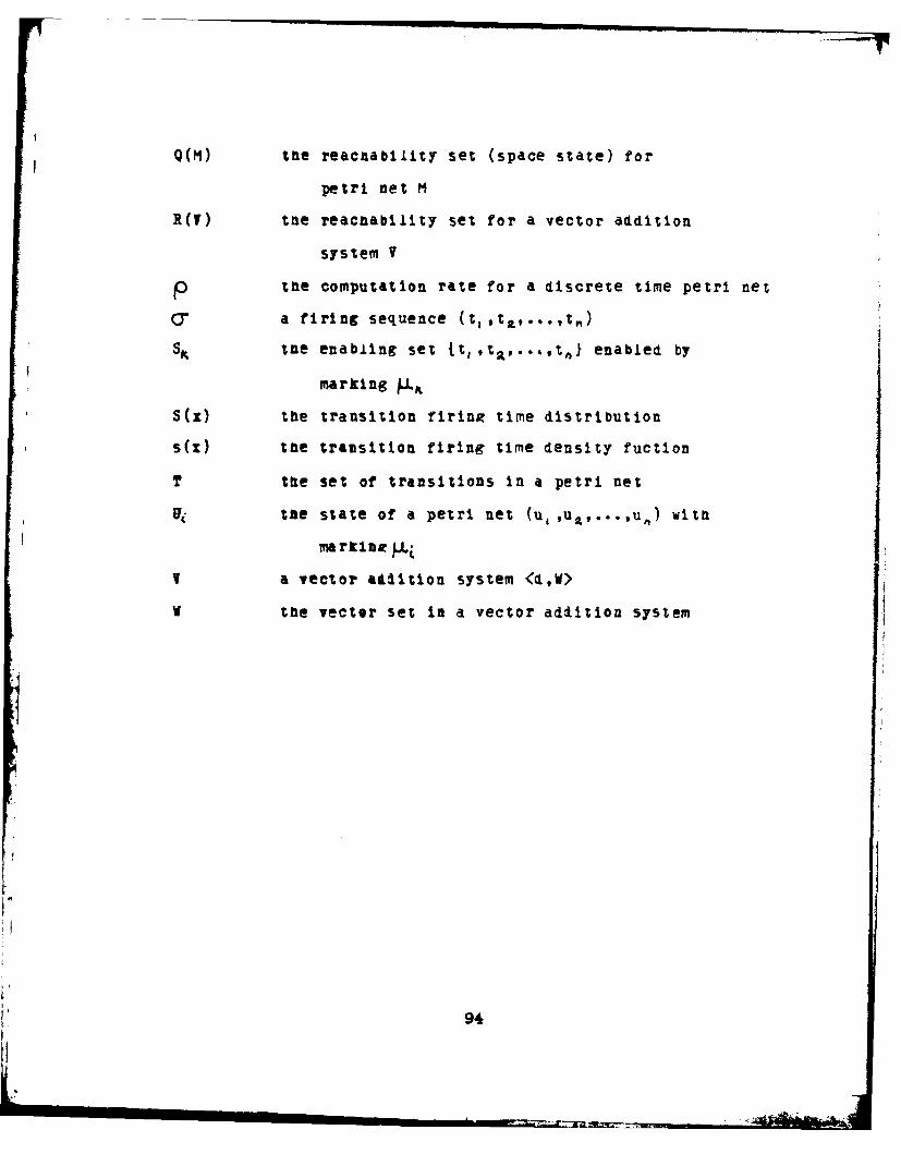
Q(M) the reacnability set (space state) for

petri net M

R(V) the reacnability set for a vector addition

system V

p the computation rate for a discrete time petri net

a firing sequence (t,t a,...,9tn)

SK tue enabling set jt ,ta,...,t,} enabled by

marking

S(W) the transition ftrinR time distribution

s(W) tne transition firing time density fuction

T the set of transitions In a petri net

Ui the state of a petri net (u, ,U,,...,u^) with

markinx w

V a vector atAition system <d,W>

V tue vector set in a vector addition system

94

LIST OF REFERENCES

1. Cox, L. A., Performance Prediction From a ComputerHardvare Descrintion, Naval Postgraduate School ReportNPS52-79-0l, December 1979

2. Anderson, a. A. and Jenson, 1. D., ComputerInterconnection Structures: Taxonomy. Cnaracteristics.and Examles, Computing Surveys, Vol 7 NO 4, December1975

3. Kobayasni, H. and [onneim, A. G., Queueing Models forComputer Communications System Analysis, IEEE TransCommunications, Vol Com-25 No 1, January 1977

4. Ferrari, D., Computer Systems Performance Evaluation,Prentice-Hall, 1978

5. Petri, C. A., Communilation mit Automaten, Scnriften desRneinisca- Vestfaiiscnen Institutes fur InstrumentelleMatnematit an der Universitat Bonn, 1962

6. Noe, J. D. and Nutt, G. j., Macro E-Nets forRepresentation of Parallel Systems, IEEE TransComputers, Vol C-22 No 8, Aurust 1973

7. Agervala, T. and Flynn, M., Comments on Capabilities,Limitations and "Correctness' of Petri Nets, Proc FirstAnnual Symp on Comp Arc, ACM, 1973

8. Ramchandani, C., knalysis of Asynctronous ConcurrentSystems by Timed Fm-tri Nets, M1T Project MAC TR-12e, PtTThesis, 1ii?4

9. Peterson, J. L., Computation Sequence Sets, J of Compand System Scd, Vo't 13, pp 1-24, 1975

19. BacK, M., Petri Net Languaees, MIT Project MAC CSG Memo124, 1974

11. Commoner, F. and Bolt, A. W., Markel Directed Graphs, JComp and System Scl, Vol 5 No 7, December 1971

12. Holt, A. W. and Commontr, F., Events ani Conditions,Record of Project MAC Cont on Concurrent Systems andParallel Computation, ACM, June 1970

13. Landveber, L. R. and Robertson, E. L., Pronerties ofConflict-Pree and Persistent Petri Netf, J of the ACM,Vol 25 No 3, July 1978

95

7 JPA1D0* 5' NAVAL POSTGRADATE SCHOOL MNtTEREY CA F/e 9/2ANALYTIC PERFOR0ANCE MODELING OF CONCURRENT C0ONPUTER SYSTEMS BY--ETC (U)JUN 81 S W SMART

NCLASSIFIED END

U2 l lf f .L

14. Misunas, D., Petri Net% and Speed Independent resitn,Comm of te ACM, Vol 16 No 8, August 1973

15. Patil, S. S. and Dennis, J. I., The Description andRealization of Digital Systems, Digest of Papers,COMPCON 72, IEES Computer Society, 1972

16.-Thornton, J. g., Design of a Comnuter: The Control Data6600, Scott, Foresman and Co, 1970

17. Cox, L. 1., Parfnrmanc@ Predtction of CombuterArrh...orl0 01.Pratifn. nn Linpar Mathimatinal ModCls,PhD Thesis, Dept of Comp Scl, University ofCalifornia--Davis, September 1978

18. Anderson, D. W. and others, Tne IlBM/3@6 Model 91:Machine Philosophy and Instruction Handling, IBM JResearch and Development, Vol 11 No 1, January 196?

19. Stowers, D. M., Comnuter Arcnitecture PerformancePrediction for Naval Fire Control Systems, MastersTnesis, Naval Postgraduate School, December 1979

28. Valette, R., Analysis of Petri Nets by StepwiseRefinements, J of Camp and System Sci, Voi 18, pp 35-45,1979

;1. Merlin, P. M., A MothadmIa s for tft Desimn and

Implementation of Communication Protocols, IEEE TransCommunications, Vol Com-24 No 6, June 1976

22. DiJrstra, E. W., Cooperating Sequentiai Processes,Protramine Languares, Genuys, F. ed., Academic Press,1968

23. Peterson, J. L., Petri Net, Computine Surveys, Vol 9 No3, September 1977

24. Karp, R. M. and Miller, R. I., Prnpprtits of a Model ForParallel ComputationA: Determinancy. Ternilatlon.

queueing, SIAM J kppl Math, Vol 14, No 6, November 1966

25. Karp, R. M. and Miller,. R. E., Parallel Pro-ram

Schemata, J of Comp and System Sc, Vol 3, pp 147-195,1969

26. Reiter, R., Scaedulini Parallel Computations, J of theACM, Vol 15 No 4, October 1968

96

27. Meyer, S. C., An Analytic Approach to PerformanceAnalysis For a Class of Data Flov Processors, Proc 1976Coanf on Parallel Processing, IEEE Computer Society, 1976

28. Miller, R. I., A comparison of Some Theoretical Modelsof Parallel Computation, IEEE Trans Computers, Vol C-22No 8, August 1973

29. JacKson, J. R., NetworKs of Vaiting Lines, OperationsResearcn, Vol 5, pp. 518-521, 1957

30. Gordon, V. J. and Newell, G. F., Closed Queueing SXstemsVitn Exponential Servers, Operations Research, Vol 15 No2, March 1467

31. JacKson, J. R., Jobshoo-Like Oueueing Systems,

Management Science, Vol 10, pp. 131-142, 19b3

32. Bastett, F. and otners, Open. Closed, and Mixed Networks

of Queues Vith Different Classes of Customers, J of theACM, Vol 22 No 2, April 1975

33. Chandy, 1. M. and others, Product Form and Local BalanceIn Queueing Networks, J of the ACM, Vol 24 No 2, April1977

34. Bater, . G., Rabin's Proof of tne Unecidability of tneReachabilitl Set Inclusion Problem of Vector AdditionSystems, MIT Project MAC CSG Memo 79, July 1973

35. Sacerdote, G. and Tenney, R. L., Tne Decidability If tnpReacability Problem for Vector Addition Systems,submitted for publication

36. Rack, M., The Recursive Equivalence of the ReacnabllityProblem and the Llveness Problem for PPtri Nets andVector Addition Systems, Proc 15tn Annual Symp onSvitching and Automata, IEEE, 1974

37. Sifatis, J., Use of Petri Nets for PerformanceEvaluation, Measuring, Modeling and Evaluating ComputerSystems, bellner, g. and Gelenbe, E. eds, North-Holland,1977

38. Zuberet, V. M., Timed Petri Nets and PreliminaryPerformance Evaluation Proc 7%n Annual Symp on CompArch, IEEE, 1989

97

39. Ramamoortay, L. V. and Ho, G. S., gerformance Evaiuationof Asynchronous Concurrent Systems Using Petri Nets,IEEE Trans Software Enaineerine, Vol SE-6 No 5,September 1990

40. [leinroct, L., Communication Nets, McGraw-Hill,1964

41. [leinroct, L., Performance Models and Measurements ofthe ARPA Computer Networ. Computer CommunicationMetworts, Grimsdale, R. L. and [uo, F. F. eds.,Noordhoff, 1975

42. Buzen, J. P., Computational Algorltnms fr Closedgueueing Netvorks with Exponential Servers,ommunications of the ACM, Vol 16 No 9, September 1973

43. Lien, T. B., Termination Properties of Generalized Petri

yjj., SIAM J 'on Computing, Vol 5 No 2, June 1975

44. Tovsley, D. F., ,Local Balance Models of ComputerSystems, PhD Thes is, Univ of Texas at Auston, December1975

45. Stewart, W. J., 4 Comparison of Numerical Techniques inMartov Modeling Communications of tfe ACM, Vol 21,February 1978

46. Chandy, K. M. and Saur, C. 3., Approximate Methods forAnalyzing OueueinR Netvork Models of Computing SystMsm,Computine Surveys, Vol 10 No 3, September 1978

98

i;

INITIAL DISTRIBUTION LIST

No Copies

1. Defense Tecnnical Information Center 2Cameron StationAlexandria, Virginia 22314

2. Library, Code 0142 2

Naval Postgraduate SchoolMonterey, California 93940

3. Department of Computer Science 4

NPS Code 52Naval Postgraduate SchoolMonterey, CA 93940

4. Professor L. A. Cox 3

NPS Code 52CLNaval Posteraduate SchoolMonterey, CA 93949

5. LT Scott V. Smart, USN 37409 IdvardNew Orleans, Louisiana 70125

6. Professor R. Hamming 2

NPS Code 521GNaval Postrraduate SchoolMonterey, CA 93940

7. Professor J. McGravDepartment of Applied ScienceUniversity of CaliforniaP.O. Box 88Livermore, CA 94550

8. Dr. J. DennisDepartment of Computer ScienceMassacausetts Institute of TecnnologyBoston, MA 02139

9. Professor J. Esary 1

MPS Code 55Naval Postgraduate SchoolMonterey, CA 93940

99