V. Ivanov, C. Adolphsen, N. Folwell, L. Ge,

A. Guetz, Z. Li, C.-K. Ng, J. W. Wang,

M. Wolf, K. Ko, SLAC;

G. Schussmann, UC Davis;

M. Weiner, Harvey Mudd College.

• Introduction– RF breakdown in accelerating structures– Dark current capture

• Methods of Calculations– Transient time domain (Tau3P)– Particle tracking (Track3P)

• Peak Field Calculations– Rise time effects

• Dark current capture– Bend waveguide– 30-cell TW structure

• High gradient structures for future linear colliders have experienced problems with– RF breakdown– dark current capture

• RF breakdown limits structures from operating at high gradients

• Dark currents change RF properties of structures and generate backgrounds to particle detectors

• We attempt to understand the mechanisms contributing to these phenomena by studying peak fields during the duration of the input pulse

NLC X-band structure showing damage in the structure cells after high power test

Time domain simulationsThe peak field in an accelerating structure is determined

by direct simulations in the time domain. Tau3P, a paralleltime domain electromagnetic code with unstructured grids, is used for

– Time domain can study transient effects of the driving pulse, in particular, field enhancement due to different rise times of thepulse

– Unstructured grid that conforms to geometry renders accurate determination of peak fields on structure walls

– Parallel computing enables end-to-end simulations of an entire accelerating section

Particle tracking simulationsUsing the time domain fields obtained from Tau3P, dark

current capture is studied by following trajectories of particles emitted from structure walls. Track3P, underdevelopment, is a 3D particle tracking code to incorporate

– Transient as well as steady state fields– All relevant surface physics

• Primary field emissions • Secondary emissions

• The peak field effects in an accelerating structure are studied as follows– Drive a pulse with a certain rise time from the input

waveguide until the system reaches steady state– Monitor the electric fields on the structure surface to obtain

the peak field and its overshoot– Evaluate the dependence of field overshoot upon rise time

• Simulated structures– 30-cell, 120o phase advance, constant impedance structure– 15-cell simplified model of H90VG5, a 82-cell, 150o phase

advance, constant gradient structure– full model of H90VG5

The 30-cell constant impedance structure and the model of the distributed mesh

The structure is driven at 11.424 GHz with different rise time at 10 ns, 20 ns, and 30ns.

Rise time = 10 ns

Drive pulse Reflection and transmission

Electric field as a function of time at different cell disks

1st cell

Rise time = 10 ns

15th cell 29th cell

The transient peak field is larger than its steady state value. The overshoot is more pronounced for smaller rise time, and is about 17% at 10 ns rise time.

Overshoots for different rise times Overshoot percentage

• From the dispersion curve, the structure bandwidth is 400 MHz.

• The smaller the rise time is, the wider the spread in the pulse bandwidth is.

• The transmission of frequency components within the structure bandwidth causes overshoots in fields.

Reflection spectrum

400 MHz

400 MHz

Dispersion diagram

Transient peak field found here

Electric field amplitude

Magnetic field amplitude

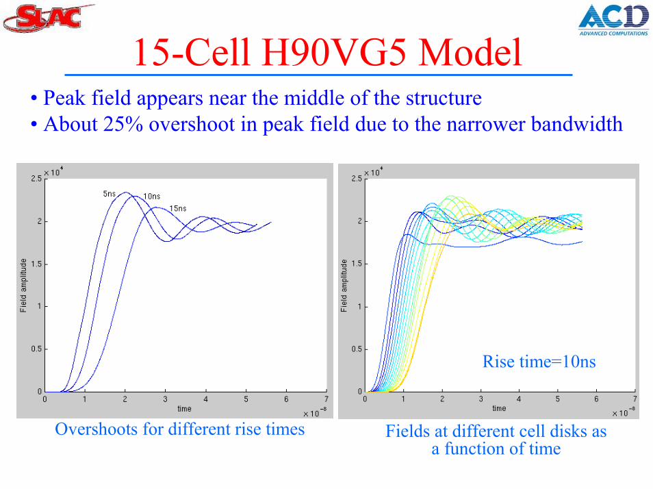
• Peak field appears near the middle of the structure• About 25% overshoot in peak field due to the narrower bandwidth

Overshoots for different rise times

Rise time=10ns

Fields at different cell disks as a function of time

Simulation Codes Tau3P & Track3P

Track3P (Particle tracking module)

using E & B fields from the parallel time-domain solver Tau3P on unstructured grid

with particle injection given by

� �22 /1

1,),1(cv

vmpBvc

Eedtpd

�

����� ����

�

�

�

�

,

.

B EtE H Jt

�� ���

�

�� �� �

�

�

�

�

� �

200

max

1)(

���

����

���

���

����

tiDtav

ItI

�

�

Surface Physics•Thermal Emission (Child – Langmuir)

• Field Emission (Fowler - Nordheim)

• Secondary emission

MdQEtrJ

2

02

94),( ��

� � ���

����

� �����

����

��

��EeEtrJ �

�

�

�

�5.191053.6252.46

1054.1),(

� = Isec/Ipri = �+�+r;

�- true secondary emission =

(0-50 eV). �m�2-4.5eV; �� �12-15 eV;

� - non elastic reflection (50 eV-�pri)

r - elastic reflection = 0.05-0.5 for metals.

Simulation results for 2D and 3D models

G = 50 MV/m

G = 100 MV/m

90 Degree Square Bend Simulation High power test on a 90 degree square bend provided measured X-ray data to allow the secondary emission model in Track3P be Benchmarked on a simple geometry

Electric field

Magnetic field

Square Bend Waveguide Used at NLCTA to Transport SLED II Output Powerto Structures

Surface Physics BenchmarkX-Ray Energy Spectrum – Good agreement between Track3P simulation and measurement indicates high energy X-Rays seen in experiments are due to elastically scattered secondary electrons.

Simulation

02468

101214161820

25000 50000 75000 100000 125000 150000E, eV

N

30-cells High-Gradient Structure• NLC X-band structure showing damage after high power test [2];

• Realistic simulation needed to understand underlying processes

Distributed model on a mesh of half million hexahedral elements for Tau3Psimulation of field evolution

Field distribution in travelling wave structure

Evolution of dark current. Red – primary particles, Green - secondaries

Dark Current Results In 30-cell Structure

0.001

0.01

0.1

1

10

100

1000

10000

100000

40 60 80 100 120 140Accelerating Gradient E, MV/m

I, mA Simulation vs measurement

Measurement: redSimulation: blue

Current in output cross-section

-30

-25

-20

-15

-10

-5

0

0 0.1 0.2 0.3 0.4 0.5t, ns

I, uA

Particle absorbed at wall vs time

00.020.040.060.080.1

0.120.140.16

0 2E-10 4E-10 6E-10 8E-10

t, s

I, A

100 0 100 200 300 400 500 600 700 800 900 10000

0.1

0.2

0.3

0.4

0.5

# of measurement

sqrt

(|S11

|)

Axial Field, P=25MW

0.00E+001.00E+072.00E+073.00E+074.00E+075.00E+076.00E+077.00E+078.00E+07

0.00E+00 1.00E-02 2.00E-02 3.00E-02 4.00E-02 5.00E-02

z, m

E, V

/m

measurement

simulation

Surface Field & Dark Current Electrons

Amplitude of surface electric field

Snapshots of primary and secondary electrons

Emitted Current vs Time

0.01.0

2.03.0

4.0

0.0E+00 1.0E-10 2.0E-10 3.0E-10 4.0E-10 5.0E-10t, s

I, A

Secondar y

Pr imar y

Current in cross-sections

-6.0E-04-5.0E-04-4.0E-04-3.0E-04-2.0E-04-1.0E-040.0E+00

0.0E+00 1.0E-10 2.0E-10 3.0E-10 4.0E-10 5.0E-10t, s

I, A

z=0

z=6

X-ray Spectrum, P=50MW

0.00E+001.00E-052.00E-053.00E-054.00E-055.00E-056.00E-057.00E-058.00E-059.00E-051.00E-04

0.00E+00 2.00E+05 4.00E+05 6.00E+05 8.00E+05 1.00E+06

E, eV

NX-ray Spectrum, P=25 MW

0.00E+00

5.00E-08

1.00E-07

1.50E-07

2.00E-07

2.50E-07

3.00E-07

0.00E+00 2.00E+05 4.00E+05 6.00E+05 8.00E+05 1.00E+06E, eV

N