UvA-DARE is a service provided by the library of the University of Amsterdam (http://dare.uva.nl)

UvA-DARE (Digital Academic Repository)

Regime shifts: early warnings

Wagener, F.O.O.

Published in:Encyclopedia of energy, natural resource, and environmental economics. - Vol. 2: Resources

DOI:10.1016/B978-0-12-375067-9.00156-X

Link to publication

Citation for published version (APA):Wagener, F. O. O. (2013). Regime shifts: early warnings. In J. Shogren (Ed.), Encyclopedia of energy, naturalresource, and environmental economics. - Vol. 2: Resources (pp. 349-359). Amsterdam: Elsevier. DOI:10.1016/B978-0-12-375067-9.00156-X

General rightsIt is not permitted to download or to forward/distribute the text or part of it without the consent of the author(s) and/or copyright holder(s),other than for strictly personal, individual use, unless the work is under an open content license (like Creative Commons).

Disclaimer/Complaints regulationsIf you believe that digital publication of certain material infringes any of your rights or (privacy) interests, please let the Library know, statingyour reasons. In case of a legitimate complaint, the Library will make the material inaccessible and/or remove it from the website. Please Askthe Library: http://uba.uva.nl/en/contact, or a letter to: Library of the University of Amsterdam, Secretariat, Singel 425, 1012 WP Amsterdam,The Netherlands. You will be contacted as soon as possible.

Download date: 27 Aug 2018

Regime shis: early warnings

Florian Wagener*

th March

A system that is at a steady state responds most of the time gradually to externalchanges. But in exceptional circumstances, it can exhibit a sudden ‘catastrophic’ shito a different regime. It is of great practical interest to develop early warning indicatorsthat signal the imminence of such a shi. A promising class of such indicators uses theuniversal fact that the average return time to a stable steady state aer a small disturb-ance increases sharply close to a catastrophic shi. It is however important to realisethat there are classes of dynamic regime shis that cannot be predicted in this way.Aer reviewing the mathematical ideas behind these indicators, this article discussestheir scope and their limitations.

Glossary

autocorrelation coefficient e first (second, third, …) order autocorrelation coeffi-cient is the correlation of the time series {xt} with the series where all elementsare one (two, three, …) step shied {xt+1} ({xt+2}, {xt+3}, …).

complex unit circle See eigenvalue.

eigenvalue A matrix can be fully described by its actions on characteristic directions.Barring exceptional cases, these are either invariant lines or invariant planes. Inthe first situation, the action of the matrix either contracts or expands the lineby a fixed factor λ, the so-called eigenvalue of the characteristic direction. Inthe second situation, the action of the matrix is first a uniform contraction orexpansion of all lines through the origin by a fixed factor r, and then a rotationaround an angle ϑ of all these lines around the origin.

It is mathematically convenient to describe the second situation in terms of com-plex numbers, as the invariant plane then becomes an invariant complex line,with an associated complex eigenvalue reiϑ. e statement that an eigenvalueis inside the complex unit circle is then equivalent to the fact that the action onthe corresponding characteristic direction is a contraction, possibly, for complexeigenvalues that are not real, followed by a rotation. If an eigenvalue is outside

*CeNDEF, Amsterdam School of Economics, Universiteit van Amsterdam, and Tinbergen Institute.E-mail: F.O.O.Wagener@uva.nl

the unit circle indicates that the action is an expansion, possibly followed by arotation.

Jacobian matrix For real-valued functions of one variable, the Jacobian matrix is justthe derivative. For a vector-valued function F = F (x), where the vector F hascomponents Fi and where x has components xj , the Jacobian matrix DF is theappropriate generalisation of the derivative. Its elements are of the form (DF )ij =∂Fi/∂xj , that is, the partial derivatives of the components of F .

smooth dependence e dependence y = f(x) of the quantity y on the quantity x issmooth, if f is a differentiable function of x for all x.

stoastic process A stochastic process is a series of random variables, indexed by atime variable.

Taylor’s theorem is is a mathematical statement about the approximation of a func-tion around a given point. In the article only a very simple version is needed. If allpartial derivatives of a map F (x) exist at a point x and are continuous functionsthere, then there is a function N(x) such that

F (x) = F (x) +DF (x)(x− x) +N(x),

and which is such thatN(x)/∥x− x∥ → 0 as x → x; here ∥x− x∥ is the distancefrom x to x. e mathematics express the fact that the difference N between thefunction F (x) and its ‘linear approximation’ F (x) +DF (x)(x − x) is more andmore negligible as x comes closer to x.

Evolution equations

Systems that evolve in time are thought of and modelled as dynamical systems. estate of the system at a given point t in time is described by a state vector xt, which isan ordered list of numbers that contains all information needed in order to describe thesystem at that particular instance in time. e length of the list is the dimension of thevector, and in practical applications the dimension of a state vector can be high. Forinstance, in a climate model, this would include the value of temperature, wind speedand pressure at many altitudes over many points on the earth surface.

Mathematically, a dynamical system consists of a set of state vectors, consti-tuting the state space, and an evolution law, which determines how the state vectorxt evolves as time changes. In a model, the evolution law describes the effect of shortterm interactions of the components of the state vector. e general aim of dynam-ical system theory is to derive from these short time interactions the long run systembehaviour.

ere are two classes of evolution equations, describing the time evolutioneither as a continuous flow or as a succession of discrete time steps. As the distinction

has no significant implications to the following discussion, this article only considersdiscrete time systems. For these systems, the short time system interactions give riseto an evolution map F . e associated evolution equation

xt+1 = F (xt) ()

governs the time path of the state. e map F is oen called ‘the dynamical system’.e initial state x0 and the evolution law F determine the evolution of a dynamicalsystem of the form (): such systems are called deterministic.

In analogy to the situation in mechanics, the quantity f(x) = F (x)−x is calledthe force acting on the system. In terms of the force, the evolution equation takes theform

xt+1 = xt + f(xt). ()

If no force is acting on the system, then the state of the system will not change: thatis, if f(xt) = 0, then xt+1 = xt for all t. e system is said to be at a steady state.

Practical systems are subject to external disturbances. ese could be intern-alised by considering a bigger system that also models the disturbance, but it is morecommon to model the disturbances as random shocks to the system. is leads to con-sidering evolution equations of the form

xt+1 = F (xt, ηt), ()

where {ηt} is a sequence of stochastic variables that model random shocks. A systemof the form () is called a stoastic dynamical system.

Typically, the evolution of a system confines itself for long periods of time toa small part of the whole state space of the system, a ‘regime’: states in a given re-gime have similar characteristics. Occasionally the system can switch to a differentregime. For instance, the earth’s climate system has shied between ‘glaciation’ and‘greenhouse’ regimes in the past.

It is of interest to be able to predict these regime shis before they actually occur,based on observations of the system. If the evolutionmapF is known, this is a questionof identifying the present state xt and to compute its future evolution. Oen, however,the evolution map is known imperfectly or not at all and the only information availableare a series of observations {xt} of the state, a so-called time series. General dynamicalsystem theory can be used to develop early warning indicators for impending regimeshis even for this situation.

Regime shis in deterministic systems

is section introduces some basic notions from general dynamical systems theory.

. Steady states

As mentioned above, if at a given state x no force acts on the system, then the systemwill not leave this state, and x is a steady state. However, a steady state is only dy-

namically relevant if it is stable. is means the following: if all state vectors that areinitially close to the steady state give rise to time evolutions of the system that tendto the steady state as time increases, the steady state is called stable, or in technicallanguage ‘locally asymptotically stable’. Unstable steady states will almost never beobserved, as in practice there are always small perturbations pushing a system out ofthe state and the system is not necessarily pushed back towards it.

To analyse the dynamics close to a steady state x, it is convenient to write thestate xt of the system as a deviation yt from the steady state, that is

xt = x+ yt. ()

In terms of deviations, the evolution equation () takes the form

yt+1 = F (x+ yt)− x. ()

is system has a steady state at yt = 0.Invoking Taylor’s theorem, and using the fact that F (x) = x at steady state,

this can be wrien asyt+1 = Ayt +N(yt), ()

where A = DF (x) is the Jacobian matrix of F at x, and where the term N(yt) istypically much smaller than the linear term Ayt when the deviation yt is close to thesteady state y = 0. Put differently, oen the dynamics of the system is already welldescribed by the ‘linear approximation’

yt+1 = Ayt. ()

A sufficient condition for the local stability of the steady state y = 0 of the system ()is that all eigenvalues of the matrixA are inside the complex unit circle. In the simplestsituation, where the state space is one-dimensional, this implies that close to the steadystate, the system is equivalent to the simple linear system

yt+1 = λyt ()

with |λ| < 1. Equivalence means here that the evolutions of the linear system closeto the steady state y = 0 are a faithful image of the evolutions close to the steadystate x of the original system; this implies that it is sufficient to consider the lineardynamics (). ose dynamics have the structure of a negative feedback loop: thequantity yt measures the displacement of the system from the steady state, and thenew displacement yt will be smaller in absolute value than yt. As yt+1 feeds back intothe right hand side of equation () when t is replaced by t + 1, it follows that thesequence of disturbances yt, yt+1, yt+2, . . . decays towards zero.

e characteristic time T of this decay is inversely related to the magnitudeof |λ|−1. More precisely, defining the characteristic time as the time needed for a dis-turbance to decay towards e−1 ≈ 0.37 times the original level, then the characteristicdecay time reads as

T =1

log |λ|−1. ()

For a stable steady state in a high-dimensional system, the characteristic time is alsogiven by equation (), but with λ replaced by the eigenvalue that is largest in absolutevalue.

If however only a single eigenvalue of the Jacobian matrix is outside the unitcircle, then the steady state is unstable. Again equation (), with |λ| > 1, can explainthis: as now the absolute value of yt is amplified at each time step by the factor |λ|, thesystem constitutes a positive feedback loop which will in time drive the system fromthe steady state.

. Parameters

Dynamical systems oen depend on parameters: think of these as state variables thatdo not change. Parameters are additional variables, separate from state variables, thatdetermine the characteristics of the system; each value of the vector of parameters thencorresponds to a different dynamical system. e totality of the systems obtained inthis way is called a (parametrised) family Fµ of systems:

xt+1 = F (xt, µ) = Fµ(xt). ()

For instance, climate models operating on historical time scales assume theearth’s axial tilt, which is the inclination of the rotation axis of the earth relative toits orbital plane, to be constant. In reality the axial tilt changes periodically over a timeperiod of approximately 41 000 years. Other examples are the terrestrial albedo or theoutput of greenhouse gases in different locations around the globe. In general, as longas the value of a quantity changes sufficiently slowly it is admissible to treat it as aparameter. In a further analysis, it can and should be treated as a slowly varying statevariable.

. Generic properties

When discussing dynamical systems without any information given about the specificstructure of the map F , it is helpful to restrict the discourse to generic properties ofsystems. Loosely speaking, these are the properties of ‘typical’ dynamical systems, orof typical families of systems.

Genericity of a propertymeans the following two things: any systemF , whetherit possesses the property or not, can be arbitrarilywell approximated by systems havingthe property: the property is said to be pervasive or dense in the space of all systems.And secondly, if a system F possesses the property, then it is not possible to makea modification to F that destroys the property, at least as long as the modification issufficiently small: the property is said to be stable or open in the space of systems. Ofcourse, the notions ‘arbitrarily well approximated’ and ‘sufficiently small’ have to bemade more precise before this definition is operational, but this is the basic idea.

For instance, for the system given in equation (), let x be a locally asymptotic-ally stable steady state of F . In the space of all systems that have a stable steady state,

the property that the eigenvalues of the Jacobian matrixDF (x) are inside the complexunit circle is a generic property.

. Loss of stability

Consider now a family Fµ of systems that depends on a real-valued parameter µ: eachparticular value of µ singles out a member of the family. Assume that Fµ0 has a stablesteady state x0 such that all eigenvalues ofDFµ0(x0) are inside the complex unit circle.

en locally around the parameter value µ0, the steady state x = x(µ) variessmoothly with the parameter µ. is rather abstract result has a concrete interpreta-tion: generically, a stable steady state responds gradually to external changes in thesurrounding conditions.

As the eigenvalues of the JacobianmatrixDFµ evaluated at the steady state x(µ)depend smoothly on µ, the steady state can only lose its stability when one of theeigenvalues crosses the complex unit circle. What happens in that situation dependson the local structure of the dynamical system at the steady state. As the structure ofthe resulting dynamics changes at a stability loss, the dynamical system is said to gothrough a qualitative change of dynamics or, more succinctly, a bifurcation.

ere are two kinds of stability loss: so and hard. Aer a so loss of stability,the system seles down to a time evolution that is still in the vicinity of the steady state.Aer a hard loss of stability, the system may evolve towards an entirely different partof the state space and an entirely different dynamical behaviour, both unpredictablefrom the previous steady state dynamics. It is clear that only a hard loss of stabilitycan induce a regime shi.

It is here that the concept of genericity turns out to be useful: whereas for arbit-rary families of systems the dynamicsmight change in amultitude of different ways, forgeneric families that depend on a single scalar parameter there are precisely three dif-ferent bifurcation scenarios through which a hard loss of stability can take place. eseare, respectively, the saddle-node, the subcritical period-doubling and the subcriticalHopf bifurcation. Moreover, there are suitable descriptions of the state space such thatthese bifurcations take place on a low-dimensional subspace, a so-called centre mani-fold, and the dynamics of the whole system is entirely determined by its restriction tothese centre manifolds: below, these dynamics will be called the ‘essential’ dynamicsof the system.

ere are three scenarios of hard stability loss that are universal to all dynamicalsystems: though the consequences are different for every system, the mathematicalmechanisms are equal. Choosing variables appropriately reduces a system at a hardloss of stability to one of three normal forms that describe the bifurcation mechanisms.

Almost all of the literature on early warning signals considers only the saddle-node bifurcation, though oen without mentioning it explicitly. e next subsectionwill treat this bifurcation in some detail. Aerwards, the distinctive features of theother two bifurcations will be touched upon briefly.

. e saddle-node bifurcation

.. Meanics of the bifurcation

A saddle-node bifurcation occurs if by varying a parameter µ, the biggest eigenvalue λ,in absolute value, of the Jacobian matrix DFµ(x) of a steady state exits the complexunit circle at the point λ = 1. In this case, the essential part of the system dynamicsis one-dimensional. Choosing variables in a certain suitable way, close to the steadystate and for parameter values µ close to the bifurcation value µc, the system takes thenormal form

yt+1 = yt + µc − µ− y2t . ()

at is, locally around the steady state the essential part G : R → R of the evolutionmap has the formG(y) = y+g(y), with restoring force g(y) = µc−µ−y2. For valuesof µ smaller than µc, there are two steady states

y1 =√µc − µ and y2 = −

√µc − µ, ()

while for µ > µc there is no steady state. It is already apparent from the changein the number of steady states that the dynamics bifurcate at the critical parametervalue µ = µc.

e Jacobian matrix of G reduces to the derivative G′, taking the values

λ1 = G′(y1) = 1− 2√µc − µ and λ2 = G′(y2) = 1 + 2

√µc − µ. ()

When µ is such that µc−µ is positive but close to 0, the value of λ1 is inside the complexunit circle, while λ2 is outside. Moreover λ1, as well as λ2, equals 1 at bifurcation.Consequently, the steady state y1 is stable, while y2 is unstable, and as µ approaches µc

from below, the ‘aractiveness’ of y1 decreases successively.For µ > µc there is no steady state le, and the normal form only indicates that

the systemwill leave the neighbourhood of y = 0 eventually, moving to a different partin state space. Figure gives the corresponding bifurcation diagram of the saddle-nodebifurcation. e set of equilibria forms a surface in the product of parameter and statespace. At a saddle-node bifurcation this surface folds back unto itself, as in Figure at µ = µc. On increasing the value of µ starting from low values, the stable and theunstable steady state merge and disappear in a saddle-node bifurcation.

Figure also shows the normal form dynamics () for a range of parametervalues. Initial states in the vicinity of the stable state lead to evolutions that movetowards the steady state, whereas evolutions starting close to the unstable state moveaway from that point. In fact, it is apparent that the basin of araction of the stablestate y1, that is the set of initial states which eventually will tend towards this state, isbounded by the unstable state y2. is basin of araction is a regime of the system, asall systems whose initial state are in the basin will eventually display the same dynamicbehaviour.

Μc

Μ

y

Figure : Bifurcation diagram of the saddle-node bifurcation. e solid line indicates stablesteady states, the broken line indicates unstable steady states. e arrows show the direction of thedynamics.

.. Resilience of the steady state

Holling () puts the difference between resilience and stability of a regime of a sys-tem as follows:

Resilience determines the persistence of relationships within a system andis a measure of the ability of these systems to absorb changes of state vari-ables, driving variables, and parameters, and still persist. In this definitionresilience is the property of the system and persistence or probability ofextinction is the result. Stability, on the other hand, is the ability of a sys-tem to return to an equilibrium state aer a temporary disturbance. emore rapidly it returns, and with the least fluctuation, the more stable it is.In this definition stability is the property of the system and the degree offluctuation around specific states the result.

More precisely, resilience R of a stable steady state is defined as the minimal size of aperturbation that will shi the system into a different basin of araction, whereas sta-bility S is the speed by which a system returns to the steady state aer a perturbation.e inverse of the characteristic time T , see (), quantifies this: S = 1/T . It turns outthat close to stability loss, both notions are closely related.

From the expressions for the stable and unstable equilibrium, it appears readilythat

R = 2√µc − µ. ()

In Figure this quantity is the distance of the unstable steady state, which bounds thebasin of araction of the stable steady state, to the stable steady state itself. Usingexpression () of the eigenvalue λ1 of the stable steady state, also the characteristic

decay time can be expressed in terms of the difference between the actual and thecritical value of the parameter:

T = − 1

log(1− 2√µc − µ)

. ()

is leads to the following relation between resilience and stability at a saddle-nodebifurcation

R = 1− e−1T ≈ 1

T= S, ()

where the approximation is beer as T takes larger values. We see that the resilience isinversely related to the characteristic decay time; put differently, close to a saddle-nodebifurcation the measures for resilience and stability are approximately equal.

Mechanical engineers have known this relation between resilience and stabil-ity of steady states for a long time. For mechanical systems, characteristic frequenciesreplace characteristic times; in their book, Catastrophe eory, Poston and Stew-art describe this in the case of a strut: “us unloaded it will go ‘ting’, moderatelyloaded ‘bong’, and near buckling point ‘boiinnggggg’. (is is eminently familiar tothe practical engineer, but should warn the general reader to prefer soprano structuresto bass.)”

.. Slowly varying parameters

To summarise: knowing that a family of system Fµ is at bifurcation if the system para-meter takes some critical value µ = µc gives information about all the systems thatare close to the bifurcating one. It is a statement about the structure of the family ofsystems Fµ, rather than about single members of this family.

A common fallacy in the interpretation of bifurcation theory is to think of theparameter µ as slowly changing in time, and not to realise that then there will be adynamic interplay between the system dynamics and the parameter dynamics. isis the province of a different theory, the field of slow-fast systems. ough closelyrelated to bifurcation theory, it studies different phenomena, like solution trajectoriesthat remain close to unstable steady states for long stretches of time.

A slow-fast system is a family Fµ of systems where the parameter µ dependson a slow time parameter τ . e slow time is related to the fast time t by

τ = εt, ()

e requirement that 0 < ε ≪ 1 is a small positive number expresses that τ is muchslower than t: one unit of t-time corresponds to ε units of τ -time. e parameter thenevolves as

µ = µ(τ), . ()

A steady state x(µ) of the system with constant parameters, where ε = 0, is usuallynot a steady state of the slow-fast system where ε > 0; it will called a ‘quasi-static’steady state in the following. e location of a quasi-static stable state evolves as x =

x(µ(τ)). In fact, the substitution () replaces the multi-dimensional parameter µ bythe single-dimensional parameter τ . Equivalently, we can think of the parameter µbeing one-dimensional, and that it moves sufficiently slowly that the state has time todecay towards the quasi-static steady state, at least, if µ is far from bifurcation. Closeto bifurcation this tracking of the quasi-static state by the actual state will break down.For it has already been seen that approaching the bifurcation, the characteristic decaytime will tend to infinity, and will therefore at a certain point be slower than the changein the system parameter. See also Figure below.

.. Catastrophic regime shis

Consider now the system () with a slowly varying parameter µ(τ) = µc+τ = µc+εt:the parametrisation is chosen such that at t = 0 the parameter µ equals the criticalvalue µc. e system then takes the form

yt+1 = εt+ yt − y2t . ()

For t < 0, the state yt remains close to the quasi-static steady state

y1(µ) =√µc − µ =

√−εt. ()

At t = 0, the system is close to y = 0, and for t > 0, the system dris away from y = 0at a rate that is linearly increasing in t. Figure illustrates this, indicating the regimeshi for an infinitely slow changing parameter by a dashed line, and the shi for amore rapidly changing parameter by connected dots. In the second case, the system isstill close to the region where the steady state used to be, while the steady state itself,and its basin of araction, have already disappeared. is is as far as the local analysis

ΜcΜHΤL

x

Figure : As µ increases, the upper steady state disappears in a saddle-node bifurcation at µ = µc.It then shis catastrophically towards a new regime.

of the saddle-node bifurcation will take us: if µ > µc, the system shis to a different

part in state space, possibly far away. is is commonly expressed by saying that thesystem readjusts to a new stable regime by going through a catastrophic regime shi.

Catastrophic system changes of this sort have been studied extensively fromthe s onward. e mathematicians René om and Christopher Zeeman pointedout that since the underlying mechanisms are universal for all dynamical systems, theyare expected to be relevant for a wide range of vastly different kinds of systems. Sincethen, many instances of such changes have been documented.

Actually, the saddle-node bifurcation described above is associated to the foldcatastrophe, which is the simplest, and therefore the most prevalent, of om’s classi-fication of elementary catastrophes.

. e subcritical bifurcations

ere are two other scenarios for a hard loss of stability, the subcritical period-doublingand the subcritical Neimark-Sacker bifurcation. In both bifurcations the steady stateloses stability through the onset of oscillations, and in both cases, a regime shi ensues.e corresponding supercritical bifurcations are so and do not give rise to a shi.

.. Subcritical period-doubling

e normal form dynamics of the subcritical period-doubling bifurcation read as

yt+1 = G(yt) = −(1 + µ)yt − y3t , ()

which is valid for values of yt and µ both close to 0. ere is only a single steadystate y = 0. For small negative values of µ this state is stable, while for positive valuesof µ it is unstable. ere is consequently a qualitative change at µc = 0. Foregoing afull analysis of the dynamics, Figure displays the summarising bifurcation diagram.For µ < µc there is a stable steady state at y = 0. An unstable periodic trajectory ofperiod two bounds its basin of araction.

A period-two trajectory is a state which under the evolution returns to itselfaer two time steps, and, consequently, each second time step. Denoting the lowerand upper bounds of the basin by yℓ and yu, then

yℓ = −√µc − µ, yu =

√µc − µ, ()

and G(yℓ) = yu and G(yu) = G(G(yℓ)) = yℓ. If the initial state y0 is equal to yu,then y1 is equal to yℓ, y2 to yu, y3 to yℓ etc. e system is said to exhibit period-two cyclic behaviour. From the expressions of yu and yℓ, it follows that the relationbetween the resilience R of the stable steady state and the parameter µ is again givenby equation ().

e derivative λ of G at the stable steady state reads as

λ = G′(y) = −1 + (µc − µ). ()

e distinctive feature of the period-doubling bifurcation is that λ approaches thevalue −1 at bifurcation, and not 1 as in the saddle-node bifurcation.

ΜcΜ

y

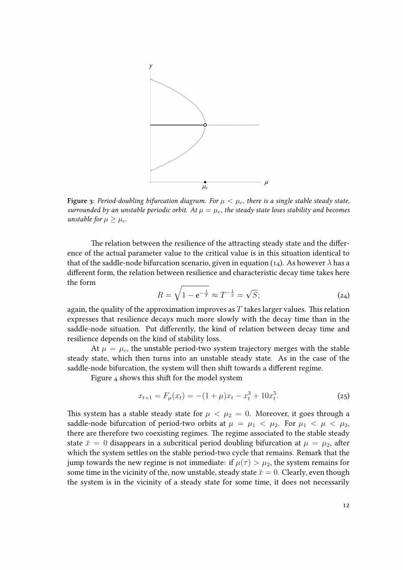
Figure : Period-doubling bifurcation diagram. For µ < µc, there is a single stable steady state,surrounded by an unstable periodic orbit. At µ = µc, the steady state loses stability and becomesunstable for µ ≥ µc.

e relation between the resilience of the aracting steady state and the differ-ence of the actual parameter value to the critical value is in this situation identical tothat of the saddle-node bifurcation scenario, given in equation (). As however λ has adifferent form, the relation between resilience and characteristic decay time takes herethe form

R =

√1− e−

1T ≈ T− 1

2 =√S; ()

again, the quality of the approximation improves as T takes larger values. is relationexpresses that resilience decays much more slowly with the decay time than in thesaddle-node situation. Put differently, the kind of relation between decay time andresilience depends on the kind of stability loss.

At µ = µc, the unstable period-two system trajectory merges with the stablesteady state, which then turns into an unstable steady state. As in the case of thesaddle-node bifurcation, the system will then shi towards a different regime.

Figure shows this shi for the model system

xt+1 = Fµ(xt) = −(1 + µ)xt − x3t + 10x5

t . ()

is system has a stable steady state for µ < µ2 = 0. Moreover, it goes through asaddle-node bifurcation of period-two orbits at µ = µ1 < µ2. For µ1 < µ < µ2,there are therefore two coexisting regimes. e regime associated to the stable steadystate x = 0 disappears in a subcritical period doubling bifurcation at µ = µ2, aerwhich the system seles on the stable period-two cycle that remains. Remark that thejump towards the new regime is not immediate: if µ(τ) > µ2, the system remains forsome time in the vicinity of the, now unstable, steady state x = 0. Clearly, even thoughthe system is in the vicinity of a steady state for some time, it does not necessarily

Μ2Μ1ΜHΤL

x

Figure : Dynamics for the system () in a (µ, x)-diagram, where µ(τ) = µc + τ = µc + εt.For µ = µ2 = 0 the system goes through a period doubling bifurcation. e system keeps traingthe unstable equilibrium for some time, before shiing to a different regime, in this case a stableperiodic orbit.

guarantee that the state is stable. is is another mechanism, again due to a slow-fastinteraction between system dynamics and parameter dynamics, how the stability lossof a steady state is apparent only aer some delay.

.. Subcritical Neimark-Saer

e last bifurcation that leads to a hard loss of stability is the subcritical Hopf or sub-critical Neimark-Saer bifurcation. e normal form map is a map G : R2 → R2 onthe plane, given as

zt+1 = (1 + µ)Uα(µ)zt + ∥zt∥2Uc(µ)zt + . . . , ()

where zt = (z1t, z2t) ∈ R2, ∥zt∥2 = z21t + z22t, and where

Uϑ =

(cosϑ − sinϑsinϑ cosϑ

)()

is thematrix of a rotation through a positive angleϑ. e bifurcation takes place atµc =0; the constants α(µc) and c(µc) have to satisfy some technical conditions, which willnot be specified, and the dots indicate terms of higher than third order in |zt| that havebeen omied. Expressing the map in polar coordinates

z1t = rt cosφt, z2t = rt sinφt, ()

and taking into account the technical conditions, the map takes the form

rt+1 = rt + rt(µ+ r2t + . . .

),

φt+1 = φt + α(µ) + β(µ)r2t + . . . .

is time, the dots indicate terms of order four or more in rt and of order two or morein µ, which will be disregarded in the following. In this approximation the evolutionof rt is independent of that of φt. In particular, there is a steady state r1 = 0 that isaracting for µ < µc and repelling for µ > µc, and a second steady state r2 =

√µc − µ

that is repelling for all µ < µc and which bounds the basin of araction of the stablesteady state.

In the original two-dimensional dynamics, the unstable steady state r = r2corresponds to an unstable invariant circle

C = {z ∈ R2 : ∥z∥ =√µc − µ}, ()

which bounds the basin of araction of the stable steady state z = 0.As in the previous situation, the relation between the resilience of the stable

steady state and the characteristic decay time is given by relation ().

ΜcΜ

Re H zL

Im H zL

Figure : Neimark-Saer bifurcation diagram. For µ < µc, there is a single stable steady state,surrounded by an unstable invariant circle orbit. At µ = µc, the steady state loses stability andbecomes unstable for µ ≥ µc.

Regime shis in stoastic systems

For a practical system at this point a problem arises. Assuming that the system is ina stable steady state, we should like to have information about its resilience. Closeto bifurcation, the resilience is inversely related to the characteristic decay time. Butit is not feasible to subject a large system like, for instance, the earth’s climate to adeliberate perturbation to determine the average return time of the climate system tosteady state.

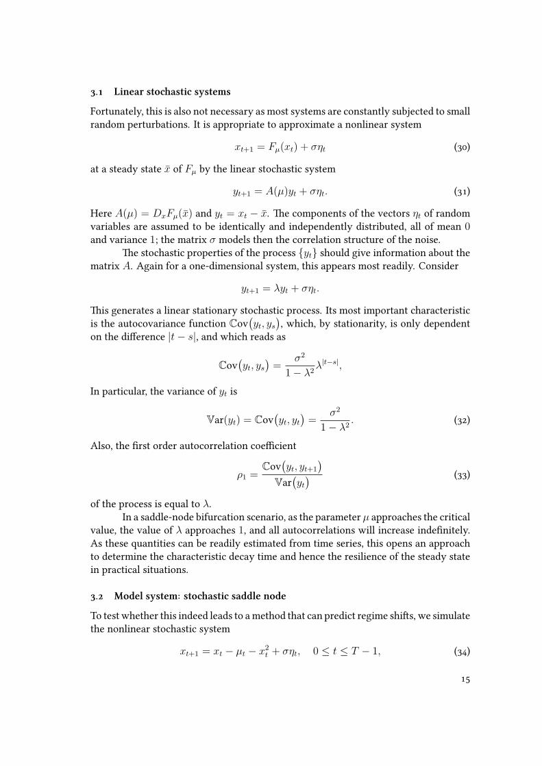
. Linear stoastic systems

Fortunately, this is also not necessary as most systems are constantly subjected to smallrandom perturbations. It is appropriate to approximate a nonlinear system

xt+1 = Fµ(xt) + σηt ()

at a steady state x of Fµ by the linear stochastic system

yt+1 = A(µ)yt + σηt. ()

Here A(µ) = DxFµ(x) and yt = xt − x. e components of the vectors ηt of randomvariables are assumed to be identically and independently distributed, all of mean 0and variance 1; the matrix σ models then the correlation structure of the noise.

e stochastic properties of the process {yt} should give information about thematrix A. Again for a one-dimensional system, this appears most readily. Consider

yt+1 = λyt + σηt.

is generates a linear stationary stochastic process. Its most important characteristicis the autocovariance function Cov

(yt, ys

), which, by stationarity, is only dependent

on the difference |t− s|, and which reads as

Cov(yt, ys

)=

σ2

1− λ2λ|t−s|,

In particular, the variance of yt is

Var(yt) = Cov(yt, yt

)=

σ2

1− λ2. ()

Also, the first order autocorrelation coefficient

ρ1 =Cov

(yt, yt+1

)Var

(yt) ()

of the process is equal to λ.In a saddle-node bifurcation scenario, as the parameter µ approaches the critical

value, the value of λ approaches 1, and all autocorrelations will increase indefinitely.As these quantities can be readily estimated from time series, this opens an approachto determine the characteristic decay time and hence the resilience of the steady statein practical situations.

. Model system: stoastic saddle node

To test whether this indeed leads to amethod that can predict regime shis, we simulatethe nonlinear stochastic system

xt+1 = xt − µt − x2t + σηt, 0 ≤ t ≤ T − 1, ()

where xt is the state variable, taking values in the real numbers, where µt is a slowlymoving parameter given as

µt = µ0 + εt, ()

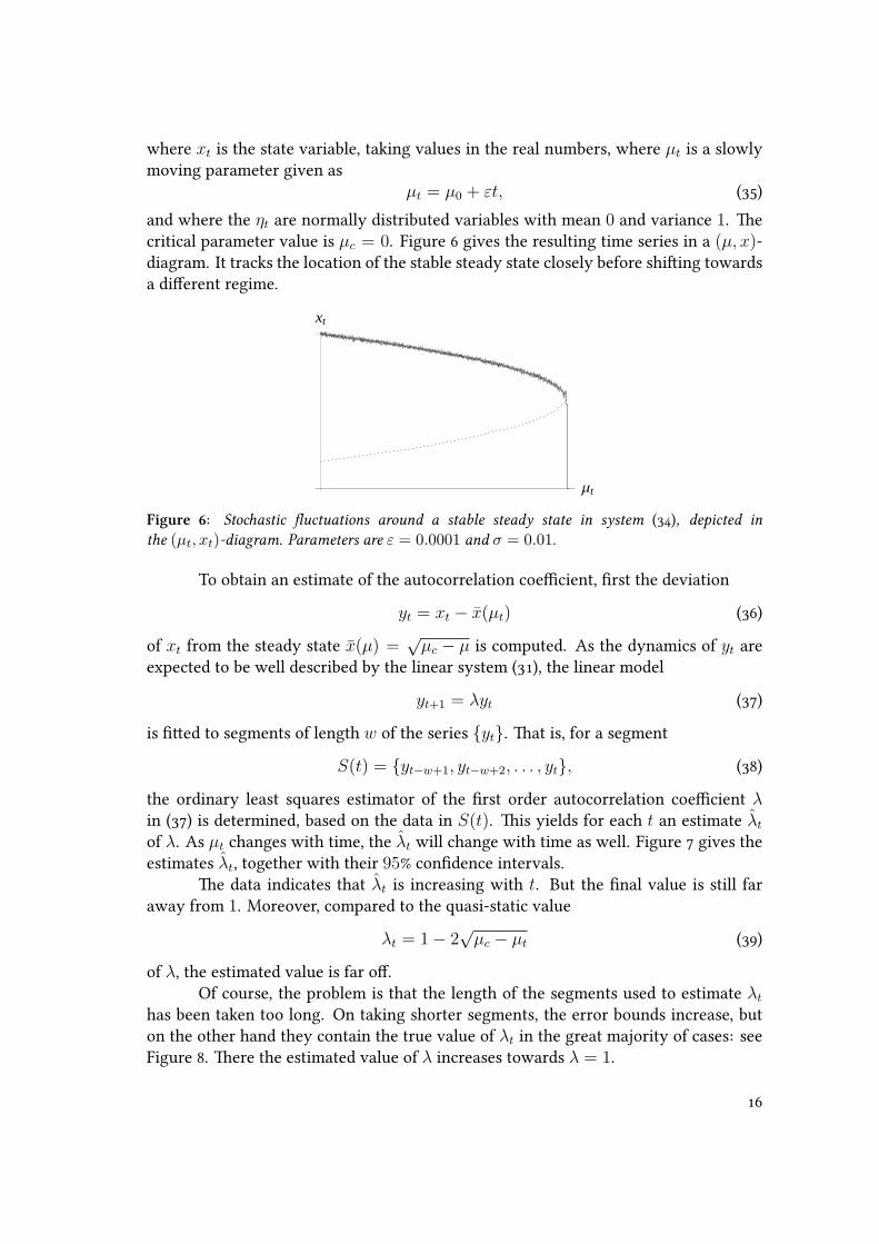
and where the ηt are normally distributed variables with mean 0 and variance 1. ecritical parameter value is µc = 0. Figure gives the resulting time series in a (µ, x)-diagram. It tracks the location of the stable steady state closely before shiing towardsa different regime.

Μt

xt

Figure : Stoastic fluctuations around a stable steady state in system (), depicted inthe (µt, xt)-diagram. Parameters are ε = 0.0001 and σ = 0.01.

To obtain an estimate of the autocorrelation coefficient, first the deviation

yt = xt − x(µt) ()

of xt from the steady state x(µ) =√µc − µ is computed. As the dynamics of yt are

expected to be well described by the linear system (), the linear model

yt+1 = λyt ()

is fied to segments of length w of the series {yt}. at is, for a segment

S(t) = {yt−w+1, yt−w+2, . . . , yt}, ()

the ordinary least squares estimator of the first order autocorrelation coefficient λin () is determined, based on the data in S(t). is yields for each t an estimate λt

of λ. As µt changes with time, the λt will change with time as well. Figure gives theestimates λt, together with their 95% confidence intervals.

e data indicates that λt is increasing with t. But the final value is still faraway from 1. Moreover, compared to the quasi-static value

λt = 1− 2√µc − µt ()

of λ, the estimated value is far off.Of course, the problem is that the length of the segments used to estimate λt

has been taken too long. On taking shorter segments, the error bounds increase, buton the other hand they contain the true value of λt in the great majority of cases: seeFigure . ere the estimated value of λ increases towards λ = 1.

3000 4000 5000t

-0.4

-0.2

0.2

0.4

0.6

0.8

Λ

Figure : Estimates λt of the first order autocorrelation coefficientλ, with 95% confidence intervals.e dashed curve indicates λt = 1− 2

√−µt. Parameters: ε = 0.0001, σ = 0.01 and w = 2500.

1000 2000t

-0.2

0.2

0.4

0.6

Λ

Figure : As in figure , but with w = 250.

. e end of the last glaciation period

Using the same techniques, we examine a temperature time series obtained from ana-lysing the Vostok ice core data. Figure shows a segment of this time series. esudden warming of the earth climate that started around , years ago is clearlyvisible.

A problem here is that the steady state x(µ) is unknown. But this can be re-solved by filtering out the high frequency oscillations to obtain a low-frequency com-ponent xt of the time series, and then subtracting out the low-frequency component toobtain

yt = xt − xt. ()

Again a linear model () is estimated over segments S(t) of lengthw. Figure depictsthe resulting estimates λt.

is seems to result in a sequence that is increasing, and a rank correlation testdoes amply confirm that. However, the subsequent estimates λt are highly dependenton each other. Moreover, the vertical scale in figure is distorted. Figure (a) givesa version with larger scale and error bounds. ere the increase in λt is far less pro-nounced. What is true, however, is that the value of λt is uniformly near the value 1.Together, this suggests that towards the end of the last glaciation period the earth cli-

5×104 2.5×104t

-8

-6

-4

-2

2DT

Figure : Temperature dynamics at the end of the last glaciation period. Time is given in years topresent, temperature as temperature difference to present day mean temperature. From Petit et al.().

3 ×104 2 ×104t

0.88

0.9

Λ

Figure : Estimates λt of the first order autocorrelation coefficient λ. Parameters: T = 911and w = 455.

mate system was in a steady state whose resilience was small. However, the evidenceof Figure (a) points against the hypothesis that the transition mechanism that led tothe present state was a catastrophic shi.

Estimates performed with a smaller time window seem to confirm this, as theincrease over time of λt is replaced by oscillatory behaviour, as in Figure (b).

. Noise-induced regime shis

Recall that the resilience of a steady state is the smallest distance of the steady stateto a point on the boundary of its basin of araction. If this quantity is of the sameorder of magnitude as σ, then there is a sizable probability that a single large shock,or a succession of medium-sized ones, may push the system outside the basin. isis a different mechanism how a system can change regimes; it is commonly called anoise-induced regime shi.

Figure (a) illustrates such a transition for the model system (). Figure (b)gives the corresponding estimates of λt for times just prior to the shi. ough the

3 ×104 2 ×104t

0.7

0.8

0.9

1

Λ

(a) w = 455

4 ×104 3 ×104 2 ×104t

0.7

0.8

0.9

1

Λ

(b) w = 250

Figure : Estimates λt of the first order autocorrelation coefficientλ, together with 95% confidenceintervals, for w ≤ t ≤ 911. Le: w = 455, right: w = 250.

500 1000 1500 2000 2500t

-0.4

-0.2

0.2

0.4

0.6

0.8xt

(a) Dynamics

500 1000 1500 2000t

-0.2

0.2

0.4

0.6

0.8

1.

Λ

(b) Autocorrelations

Figure : Le: stoastic fluctuations around a stable steady state in system (), depicted inthe (t, xt)-diagram. A broken curve denotes the location of the unstable steady state that boundsthe regime. At the noise-induced transition, the system leaves the regime. Parameters are ε =0.0001 and σ = 0.1. Right: autocorrelations with 95% confidence intervals, computed on segmentsof length w = 250.

values of λt increase, fiing and extrapolating a functional relationship of the form

λ = C√

µc − (µ0 + εt) ()

would result in a prediction for the catastrophic regime shi for values of t about 2500,whereas the noise-induced shi already occurred for t ≈ 2150.

Comparing Figures and (b) to Figures (a) and (b), it seems probable thatthe end of the last glaciation period was brought about by a noise-induce transition.

. Global bifurcations

All of the above argumentation presupposes that the system is at or near a steady state.ere are however other types of dynamic system behaviour. For instance, a systemcan oscillate regularly with one ore more frequencies: the evolution of the system then

converges to a set in state space, an aractor, which is equivalent to a circle or a torus,that is, a Cartesian product of circles. Another possibility is that a system oscillateschaotically: the aracting set is then a strange aractor, an intricate fractal set carryingcomplex dynamics. In this context, aotic refers to the phenomenon that trajectorieswhich have very similar initial conditions almost always diverge from each other andeventually generate wildly different time series: chaotic systems are unpredictable inthe long run.

e resilience of these aractors can be defined as before as the smallest per-turbation that can push some point on the aractor out of the aractors basin of at-traction. As in the case of aracting steady states, the resilience drops down to zerowhen the aractor touches the boundary of its basin of araction: the system is thensaid to go through a basin-boundary collision or a global bifurcation.

e point relevant for the present discussion is the following: contrary to steadystates, general dynamic aractors have non-trivial internal dynamics. A system atsteady state is at rest, and only changes its state if it is perturbed from its steady state:the autocorrelations of the associated time series give information about the charac-teristic return time. A system that is on a dynamic aractor is perpetually in motion,even if not perturbed, and it is a hard filtering problem to decompose the time seriesof such a system in a component corresponding to the internal dynamics and a com-ponent that is generated by perturbations away from the aractor; only the laer willgive information about the characteristic return time and the resilience of the system.In order to perform this decomposition, the strange aractor and its internal dynam-ics have to be estimated from the data. To obtain significant estimates in this manner,usually long time series of observations are needed.

A failure to take the possibility of global bifurcations into account can resultin unexpected behaviour, treating for instance a time series coming from a strangearactor as if it were generated by a noisy system at a steady state. In the follow-ing example, a time series with vanishing first order autocorrelations is generated bythe internal dynamics of an aractor in a deterministic, but chaotic, one-dimensionaldynamical system. An observer assuming that a noisy system at a steady state gen-erated the series and estimating the autocorrelations will conclude that the system isfar from bifurcation. e dynamics is however critical: changing the parameter by asmall amount, the chaotic dynamics loses the property of being aracting, and it es-capes to a different region. In this case there is no warning signal given by increasingautocorrelations.

e example considers a deterministic evolution

xt+1 = Fµ(xt) ()

on a one-dimensional state space given as

Fµ(x) =

µx(1− x), x ≥ 0,

2e2µx

e2µx + 1− 1, x < 0.

()

Figure represents the evolution law graphically. Recall that intersections of thegraph xt+1 = Fµ(xt) and the line xt+1 = xt yield steady states of the system. e cru-

-1.0 -0.5 0.5 1.0xt

-1.0

-0.5

0.5

1.0

xt+1

Figure : Evolution law () for µ = 4. White dots indicate unstable steady states, bla dotsstable steady states. If 0 ≤ x0 ≤ 1, then 0 ≤ xt ≤ 1 for all t ≥ 0.

cial property is that for 0 ≤ µ ≤ 4 the local maximum ofFµ at the critical point c = 1/2is smaller than or equal to 1. is implies that if 0 ≤ x0 ≤ 1, then the inequalit-ies 0 ≤ xt ≤ 1 will also hold for all future states xt. If however µ > 4, there is a smallinterval I around c such that if xt0 ∈ I for some t0, then xt0+1 > 1, xt0+2 < 0 and xt

tends to the stable steady state x = −1.is is another kind of catastrophic shi. Figure illustrates the correspond-

ing time series: as for µ = 4 the dynamics cannot escape from the interval [0, 1] theoscillations will go on indefinitely in that case. For µ > 4, the dynamics escapes foralmost all initial values from the interval [0, 1], sooner or later, and ends up at the stablesteady state that is close to x = −1.

250 500 750 1000t

-1.

-0.5

0.5

1.xt

250 500 750 1000t

-1.

-0.5

0.5

1.xt

Figure : Time series of the deterministic system () for µ = 4 (le) and µ = 4.00001 (right).To the casual observer, these time series may seem to be stoastic.

However, estimates of the first order autocorrelation coefficient yield a valueof almost zero in both cases, and the series that exhibits a catastrophic shi has noincrease in the autocorrelations before the shi. See Figure .

300 400 500 600 700t

-0.2

-0.1

0.1

0.2

Λ

300 400 500 600 700t

-0.2

-0.1

0.1

0.2

Λ

Figure : Autocorrelations estimated on the time series of the deterministic system () for µ = 4(le) and µ = 4.00001 (right). Window length w = 250.

Conclusion

Imminent catastrophic regime shis may be predicted from the rise of characteristicdecay times, or, equivalently, from the increase of first order autocorrelation coeffi-cients towards 1. is indicator by itself is crude: a rise gives a strong indication ofan impending regime shi, but it may overestimate the time to the regime change ifthe parameter changes quickly (Figures and ), if the estimation windows are large(Figure ), or if the stochastic perturbations are large (Figures and ). Moreover,if the indicator is far from the critical value, the system may still be close to a regimeshi (Figure ).

is should not give the impression that this method is impractical. On the con-trary, the hallmark of a scientific theory is that it gives strong and testable implications.If estimated autocorrelations exhibit the square-root type of growth of equation (),this strongly points to a catastrophic regime shi at

tc =µc − µ0

ε. ()

e counterexamples given emphasise that there are other types of regime shis thatare not picked up by the indicator. e glaciation example suggests that other mechan-isms may be beer explanations for a given shi. Moreover, the absence of a trend inthe first order autocorrelation coefficient, or even their vanishing, does not necessarilyimply a large resilience of the system.

Considering the possibility of a regime shi in, for instance, the climate systemof the earth, it is perhaps worthwhile to point out that there we know that a systemparameter – the amount of greenhouse gases in the earth’s atmosphere – is increasing,and that we have data on this increase. is gives more information to a statisticalprocedure, as the parameter ε, the speed of increase of the system parameters, can beestimated much more precisely. Moreover, the increase is presumably rapid comparedto the natural climate dynamics, which makes the probability of a catastrophic regimeshi, as opposed to a noise-induced shi, much larger. Based on the techniques presen-ted, a statistical theory of early warning signals for such a shi can be built. However,for shis that are associated to global bifurcations of more complex aractors thansteady states, more sophisticated methods have to be developed.

Further reading

Carpenter, S.R. and Brock,W.A., Rising variance: a leading indicator of ecologicaltransition, Ecology Leers, , -.

Dakos, V., Scheffer, M., van Nes, E.H., Brovkin, V., Petoukhov, V. and Held, H.,Slowing down as an early warning signal for abrupt climate change, PNAS, ,-, .

Held, H. and Kleinen, T., Detection of climate system bifurcations by degeneratefingerprinting, Geophysical Resear Leers, , L, .

Holling, C.S., Resilience and stability of ecological systems, Annual Review ofEcology and Systematics, , -, .

Petit, J.R., et al., Vostok Ice Core Data for , Years, IGBP PAGES/World DataCenter for Paleoclimatology Data Contribution Series #-. NOAA/NGDCPaleoclimatology Program, Boulder CO, USA, .

Poston, T. and Stewart, I., Catastrophe theory and its applications, London, Pitman,.

Scheffer, M., Critical transitions in nature and society, Princeton University Press,Princeton, .

Scheffer, M., Bascompte, J., Brock, W.A., Brovkin, V., Carpenter, S.R., Dakos, V.,Held, H., van Nes, E.H., Rietkerk, M. and Sugihara, G., Early-warning signals forcritical transitions, Nature, , -, .

ompson, J.M.T. and Sieber, J., Climate tipping as a noisy bifurcation: a predict-ive technique, IMA Journal of Applied Mathematics, , -, .