UvA-DARE (Digital Academic Repository) Essays on … · Essays on Nonlinear Evolutionary Game...

UvA-DARE is a service provided by the library of the University of Amsterdam (http://dare.uva.nl)

UvA-DARE (Digital Academic Repository)

Essays on nonlinear evolutionary game dynamics

Ochea, M.I.

Link to publication

Citation for published version (APA):Ochea, M. I. (2010). Essays on nonlinear evolutionary game dynamics Amsterdam: Thela Thesis

General rightsIt is not permitted to download or to forward/distribute the text or part of it without the consent of the author(s) and/or copyright holder(s),other than for strictly personal, individual use, unless the work is under an open content license (like Creative Commons).

Disclaimer/Complaints regulationsIf you believe that digital publication of certain material infringes any of your rights or (privacy) interests, please let the Library know, statingyour reasons. In case of a legitimate complaint, the Library will make the material inaccessible and/or remove it from the website. Please Askthe Library: http://uba.uva.nl/en/contact, or a letter to: Library of the University of Amsterdam, Secretariat, Singel 425, 1012 WP Amsterdam,The Netherlands. You will be contacted as soon as possible.

Download date: 27 May 2018

http://dare.uva.nl/personal/pure/en/publications/essays-on-nonlinear-evolutionary-game-dynamics(bda60fae-f957-4d08-8f2f-7975bafef7fa).html

Essays on NonlinearEvolutionary Game Dynamics

Essays on

Non

linea

r Evolution

ary G

am

e Dyn

am

ics Mariu

s Och

ea

Marius Ochea

Universiteit van Amsterdam

Research Series

Evolutionary game theory has been viewed as an evolutionary“repair” of rational actor game theory in the hope that a population of boundedly rational players may attain convergence to classic“rational” solutions, such as the Nash Equilibrium, via some learning or evolutionary process.In this thesis the model of boundedly rational players is a perturbed version of the best-reply choice, the so-called Logit rule.With the strategic context varying from models of cyclicalcompetition (Rock-Paper-Scissors), through industrial organization (Cournot) and to collective-action choice (Iterated Prisoner’sDilemma), we show that the Logit evolutionary selection among boundedly rational strategies does not necessarily guaranteeconvergence to equilibrium and a richer dynamical behavior- e.g. cycles, chaos - may be the rule rather than the exception. Marius-Ionut Ochea (1977) holds a M.A. in Economics fromCentral European University, Budapest, Hungary (2004) and a M.Phil. in Economics from Tinbergen Institute, Amsterdam, the Netherlands (2006). In 2006 he joined CeNDEF (Center for Nonlinear Dynamics in Economics and Finance) at the University of Amsterdam for his Ph.D. study. As of September 2009 he is working as a post-doc researcher at CentER, Tilburg University. Main research interests include:evolutionary game dynamics, norms evolution and emergence of cooperative behavior.

468

ISBN 978 90 5170 688 8

Cover design: Crasborn Graphic Designers bno, Valkenburg a.d. Geul

This book is no. 468 of the Tinbergen Institute Research Series, established

through cooperation between Thela Thesis and the Tinbergen Institute.

A list of books which already appeared in the series can be found in the back.


ACADEMISCH PROEFSCHRIFT

ter verkrijging van de graad van doctor

aan de Universiteit van Amsterdam

op gezag van de Rector Magni�cus

prof. dr. D.C. van den Boom

ten overstaan van een door het college voor promotie ingestelde

commissie, in het openbaar te verdedigen in de Agnietenkapel

op dinsdag 19 januari 2010, te 14.00 uur

door

Marius Ionut Ochea

geboren te Vaslui, Roemenië

Promotiecommissie:

Promotor: Prof. Dr. Cars H. Hommes

Overige leden: Prof. Dr. Josef Hofbauer

Prof. Dr. Aart de Zeeuw

Dr. Roald Ramer

Dr. Jan Tuinstra

Faculteit Economie en Bedrijskunde

Acknowledgements

It may not come as great surprise to say that, some 5 years ago, when I was joining

the Tinbergen Institute with the purpose of pursuing doctoral research, I had only

limited insight into what the actual topic of my dissertation would eventually look

like. I would have probably found some words in the current title of this thesis very

strange and exotic. Beyond a broad interest in the scienti�c adventure, the concrete

pathmarks were yet to be determined. TI M.Phil �rst year programme proved �exible

enough to allow me roam around the institute academic diversity and make a �rst

contact with CeNDEF researchers during lectures on nonlinear dynamics, bounded

rationality or evolutionary game theory. From the outset, I want to express my entire

gratitude to Cars, Jan and Roald for awakening my interest towards these research

paths. Later on, I was glad to apply to a PhD position at CeNDEF and start working

on a project that combines exactly these three lines of investigation. My dissertation

emerged out of this process.

It is perhaps di¢ cult to strike the right tone when looking back in time at people

that marked my experience as a doctoral student. First, it was a great privilege to

have Prof. Cars Hommes as my supervisor: not only for the role his advice played

on structuring and disciplining my pretty chaotic way of doing research but also

his constant support and encouragements throughout the thesis-writing process. His

friendly attitude, dedication, extensive feedback and minutely reading of my earlier

drafts were decisive for the timely and successful completion of the thesis.

I am also thankful to the members of my thesis committee. I had stimulating

v

conversations with Prof. Josef Hofbauer on earlier versions of Chapter 2 and some

extensions in that chapter originate from his suggestions. Jan Tuinstra commented

at length on Chapter 3 whereas Chapter 4 was initiated out of our discussions. Roald

Ramer introduced me to the �eld of evolutionary game dynamics and we had innu-

merous exchanges of ideas on various applications of the evolutionary theory ranging

from language to preferences evolution. Aart de Zeeuw gave me the opportunity to

continue work on repeated Prisoner�s Dilemma done in Chapter 5 and engage in post-

doctoral work on the emergence and evolution of institutions sustaining cooperation

at the international level.

At various stages of my research I have also bene�ted a lot from interaction and

very kind advise from a scienti�cally heterogenous group of researchers as CeNDEF

is: Dave, Cees, Florian, Pim, Maurice, Misha, Stelios. For the lively and friendly

environment I enjoyed in the group, my gratitude goes also to former or current

CeNDEF doctoral students: Pietro, Valentyn, Peter, Saeed, Tatiana, Domenico,

Paolo, Te. O¢ cemates are a sort of a peculiar species in research and I would

like to thank Pim, not only for our almost daily debates on almost any subject

one could think of, but also for his virtually unlimited availability for exploring the

local (experimental) music scene at, among others, STEIM or DNK Amsterdam.

Outside CeNDEF, I would also want to mention former colleagues and friends from

Tinbergen Institute: Antonio, Sumendhu, Alex, Aufa, Robert, Ana, Sumedha, Sebi,

Razvan,Vali, Marcel, Mario, Jonneke, Tse-Chun. They all turned my early transition

and stay in Amsterdam into smooth and pleasant experiences.

I could not complete this short review without thanking my parents for their

patience and understanding towards my always too rare and too short trips home

since my departure abroad. This thesis is heartly dedicated to them.

Amsterdam, November 2009

vi

Contents

Contents vii

List of Tables xi

List of Figures xiii

1 Introduction 1

1.1 Literature on convergence of game dynamics . . . . . . . . . . . . . . 4

1.2 Literature on complicated game dynamics . . . . . . . . . . . . . . . 5

1.3 Thesis Outline . . . . . . . . . . . . . . . . . . . . . . . . . . . . . . . 7

1.3.1 Multiple Steady States, Limit Cycles and Chaotic Attractors

in Logit Dynamics . . . . . . . . . . . . . . . . . . . . . . . . 8

1.3.2 Heterogenous Learning Rules in Cournot Games . . . . . . . . 10

1.3.3 On the Stability of the Cournot Solution: An Evolutionary Ap-

proach 11

1.3.4 Evolution in Iterated Prisoner�s DilemmaGames under Smoothed

Best-Reply Dynamics . . . . . . . . . . . . . . . . . . . . . . . 12

2 Multiple Steady States, Limit Cycles and Chaotic Attractors in

Logit Dynamics 15

2.1 Introduction . . . . . . . . . . . . . . . . . . . . . . . . . . . . . . . . 15

2.1.1 Motivation . . . . . . . . . . . . . . . . . . . . . . . . . . . . . 15

vii

2.1.2 �Replicative�vs. �rationalistic�dynamics . . . . . . . . . . . . 18

2.2 The Logit Dynamics . . . . . . . . . . . . . . . . . . . . . . . . . . . 19

2.2.1 Evolutionary dynamics . . . . . . . . . . . . . . . . . . . . . . 19

2.2.2 Discrete choice models-the Logit choice rule . . . . . . . . . . 21

2.3 Hopf and degenerate Hopf bifurcations . . . . . . . . . . . . . . . . . 23

2.4 Three strategy games . . . . . . . . . . . . . . . . . . . . . . . . . . . 26

2.4.1 Rock-Scissors-Paper Games . . . . . . . . . . . . . . . . . . . 27

2.4.2 Coordination Game . . . . . . . . . . . . . . . . . . . . . . . . 39

2.5 Weighted Logit Dynamics(wLogit) . . . . . . . . . . . . . . . . . . . 52

2.5.1 Rock-Scissors-Paper and wLogit Dynamics . . . . . . . . . . . 52

2.5.2 Schuster et al.(1991) Game and wLogit Dynamics . . . . . . . 55

2.6 Conclusions . . . . . . . . . . . . . . . . . . . . . . . . . . . . . . . . 58

2.A Rock-Scissor-Paper game with Logit Dynamics: Computation of the

�rst Lyapunov coe¢ cient . . . . . . . . . . . . . . . . . . . . . . . . . 59

3 Heterogenous Learning Rules in Cournot Games 61

3.1 Introduction . . . . . . . . . . . . . . . . . . . . . . . . . . . . . . . . 61

3.2 Standard Static Cournot Analysis . . . . . . . . . . . . . . . . . . . . 64

3.3 Heterogenous Learning Rules . . . . . . . . . . . . . . . . . . . . . . 65

3.3.1 Adaptive Expectations . . . . . . . . . . . . . . . . . . . . . . 65

3.3.2 Fictitious Play . . . . . . . . . . . . . . . . . . . . . . . . . . 66

3.3.3 Weighted Fictitious Play . . . . . . . . . . . . . . . . . . . . . 66

3.4 Evolutionary Cournot Games . . . . . . . . . . . . . . . . . . . . . . 67

3.4.1 Adaptive Expectations vs. Rational/Nash play . . . . . . . . . 67

3.4.2 Adaptive vs. Exponentially Weighted Fictitious Play . . . . . 76

3.4.3 Local stability analysis . . . . . . . . . . . . . . . . . . . . . . 78

3.4.4 Naive vs. Fictitious Play . . . . . . . . . . . . . . . . . . . . 84

3.5 Concluding Remarks . . . . . . . . . . . . . . . . . . . . . . . . . . . 87

viii

4 On the Stability of the Cournot Solution: An Evolutionary Ap-

proach 89

4.1 Introduction . . . . . . . . . . . . . . . . . . . . . . . . . . . . . . . . 89

4.2 The model . . . . . . . . . . . . . . . . . . . . . . . . . . . . . . . . . 91

4.3 Results . . . . . . . . . . . . . . . . . . . . . . . . . . . . . . . . . . . 96

4.3.1 Best-response dynamics limit, � !1 . . . . . . . . . . . . . . 97

4.3.2 Costly Rational Expectations, k > 0 and �nite � . . . . . . . . 98

4.4 Conclusions . . . . . . . . . . . . . . . . . . . . . . . . . . . . . . . . 101

5 Evolution in Iterated Prisoner�s Dilemma Games under Smoothed

Best-Reply Dynamics 103

5.1 Introduction . . . . . . . . . . . . . . . . . . . . . . . . . . . . . . . . 103

5.2 An Evolutionary Iterated PD game . . . . . . . . . . . . . . . . . . . 105

5.3 2�2 Ecologies . . . . . . . . . . . . . . . . . . . . . . . . . . . . . . . 109

5.3.1 AllD vs. TFT . . . . . . . . . . . . . . . . . . . . . . . . . . . 109

5.3.2 TFT vs. AllC . . . . . . . . . . . . . . . . . . . . . . . . . . . 111

5.3.3 AllD vs. AllC . . . . . . . . . . . . . . . . . . . . . . . . . . . 114

5.3.4 AllD vs. GTFT . . . . . . . . . . . . . . . . . . . . . . . . . . 115

5.3.5 AllD-WSLS . . . . . . . . . . . . . . . . . . . . . . . . . . . . 117

5.3.6 GTFT vs. AllC . . . . . . . . . . . . . . . . . . . . . . . . . . 120

5.3.7 GTFT vs. WSLS . . . . . . . . . . . . . . . . . . . . . . . . . 121

5.3.8 TFT vs. GTFT . . . . . . . . . . . . . . . . . . . . . . . . . . 124

5.3.9 TFT vs. WSLS . . . . . . . . . . . . . . . . . . . . . . . . . . 127

5.3.10 WSLS vs. AllC . . . . . . . . . . . . . . . . . . . . . . . . . . 128

5.3.11 Summary . . . . . . . . . . . . . . . . . . . . . . . . . . . . . 130

5.4 3�3 Ecologies . . . . . . . . . . . . . . . . . . . . . . . . . . . . . . . 132

5.4.1 AllD-TFT-AllC . . . . . . . . . . . . . . . . . . . . . . . . . . 132

5.4.2 AllD-GTFT-WSLS . . . . . . . . . . . . . . . . . . . . . . . . 135

5.4.3 AllD-GTFT-AllC . . . . . . . . . . . . . . . . . . . . . . . . . 139

ix

5.4.4 AllD-TFT-WSLS . . . . . . . . . . . . . . . . . . . . . . . . . 141

5.4.5 AllD-TFT-GTFT . . . . . . . . . . . . . . . . . . . . . . . . . 144

5.4.6 AllD-WSLS-AllC . . . . . . . . . . . . . . . . . . . . . . . . . 146

5.4.7 TFT-WSLS-AllC . . . . . . . . . . . . . . . . . . . . . . . . . 148

5.4.8 TFT-GTFT-WSLS . . . . . . . . . . . . . . . . . . . . . . . . 150

5.4.9 Summary . . . . . . . . . . . . . . . . . . . . . . . . . . . . . 152

5.5 4�4 ecologies . . . . . . . . . . . . . . . . . . . . . . . . . . . . . . . 153

5.5.1 No TFT . . . . . . . . . . . . . . . . . . . . . . . . . . . . . . 153

5.5.2 No AllD . . . . . . . . . . . . . . . . . . . . . . . . . . . . . . 156

5.5.3 No GTFT . . . . . . . . . . . . . . . . . . . . . . . . . . . . . 159

5.5.4 No WSLS . . . . . . . . . . . . . . . . . . . . . . . . . . . . . 161

5.5.5 No AllC . . . . . . . . . . . . . . . . . . . . . . . . . . . . . . 163

5.5.6 Summary . . . . . . . . . . . . . . . . . . . . . . . . . . . . . 165

5.6 5�5 Ecology . . . . . . . . . . . . . . . . . . . . . . . . . . . . . . . . 166

5.6.1 Numerical Bifurcation Curves . . . . . . . . . . . . . . . . . . 170

5.7 Conclusions . . . . . . . . . . . . . . . . . . . . . . . . . . . . . . . . 172

5.A Iterated PD Game-stationary distributions and average payo¤s . . . . 173

6 Summary 181

Bibliography 185

Samenvatting - summary in Dutch 195

x

List of Tables

2.1 Coordination Game, Replicator Dynamics�Long-run average �tness . 42

4.1 Linear n-player Cournot game with costly Rational expectations - In-

stability Thresholds . . . . . . . . . . . . . . . . . . . . . . . . . . . . 99

5.1 Summary dynamics 2x2 ecologies . . . . . . . . . . . . . . . . . . . . 130



5.4 Stationary distributions and average payo¤s for IPD . . . . . . . . . . 178

xi

List of Figures

2.1 Rock-Scissors-Paper and Replicator Dynamics . . . . . . . . . . . . . 31

2.2 RSP Game, Logit Dynamics-Hopf scenario, � . . . . . . . . . . . . . 33

2.3 RSP Game, Logit Dynamics-Hopf scenario, � . . . . . . . . . . . . . . 34

2.4 Rock-Scissors-Paper and Logit Dynamics: Hopf curves . . . . . . . . 35

2.5 Generalized Rock-Scissors-Paper - curves of LP and H bifurcations . . 38

2.6 Coordination Game and Replicator Dynamics - Invariant manifolds . 40

2.7 Coordination Game and Replicator Dynamics - Basins of attraction . 42

2.8 Coordination Game, " = 0:1 and Logit Dynamics - Multiple steady

states . . . . . . . . . . . . . . . . . . . . . . . . . . . . . . . . . . . 44

2.9 Coordination Game, " = 0:1 and Logit Dynamics - Moderate � . . . . 45

2.10 Coordination Game, Logit Dynamics - Equilibria curves . . . . . . . . 47

2.11 Coordination Game, Logit Dynamics - Limit point curves . . . . . . . 48

2.12 Coordination Game (" = 0:1) and Logit Dynamics�Basins of Attraction 49

2.13 Coordination Game (" = 0:6) and Logit Dynamics�Basins of Attraction 50

2.14 Coordination Game and Logit Dynamics-Long-Run Welfare . . . . . 51

2.15 RSP Game and Weighted Logit Dynamics . . . . . . . . . . . . . . . 54

2.16 Schuster et. al. (1991) game and iLogit Dynamics-Period-Doubling

route to chaos . . . . . . . . . . . . . . . . . . . . . . . . . . . . . . . 56

2.17 Schuster et. al. (1991) game and iLogit Dynamics-Strange Attractor . 57

3.1 Cournot duopoly with Adaptive and Rational players - Time series . 74

xiii

3.2 Cournot duopoly with Adaptive and Rational players - Bifurcations,

Strange Attractors . . . . . . . . . . . . . . . . . . . . . . . . . . . . 75

3.3 Cournot duopoly game with Adaptive and Weighted Fictitious Play

behaviors - Time series . . . . . . . . . . . . . . . . . . . . . . . . . . 81


behaviors - Bifurcations . . . . . . . . . . . . . . . . . . . . . . . . . 82


behaviors-Strange Attractors . . . . . . . . . . . . . . . . . . . . . . . 83

3.6 Cournot duopoly game with Naive and Fictitious Play Heuristics -

Time Series . . . . . . . . . . . . . . . . . . . . . . . . . . . . . . . . 85

3.7 Cournot duopoly game with Naive and Fictitious Play Heuristics -

Attractors . . . . . . . . . . . . . . . . . . . . . . . . . . . . . . . . . 86

4.1 Linear n-player Cournot game with Adaptive and Rational players . . 95

4.2 Linear n-player Cournot game with costly Rational expectations . . . 100

5.1 Unconditional defectors (AllD) vs. Reciprocators (TFT) . . . . . . . 111

5.2 Reciprocators(TFT) vs Unconditional Cooperators(AllC) . . . . . . . 113

5.3 Unconditional defectors (AllD) vs. Unconditional cooperators(AllC) . 115

5.4 Unconditional defectors (AllD) vs. Generous reciprocators (GTFT) . 117

5.5 Unconditional defectors(AllD) vs. Pavlov(WSLS) . . . . . . . . . . . 119

5.6 Generous reciprocators(GTFT) vs. Unconditional cooperators(AllC) . 121

5.7 Generous reciprocators (GTFT) vs. Pavlovian(WSLS) . . . . . . . . 123

5.8 Reciprocators(TFT) vs. Generous reciprocators(GTFT) . . . . . . . . 126

5.9 Reciprocators (TFT) vs. Pavlov(WSLS) . . . . . . . . . . . . . . . . 127

5.10 Pavlov (WSLS) vs. Unconditional cooperators (AllC . . . . . . . . . 129

5.11 AllD vs. TFT vs. AllC . . . . . . . . . . . . . . . . . . . . . . . . . . 134

5.12 AllD vs. GTFT vs. WSLS - Bifurcations, Phase plots . . . . . . . . . 137

5.13 AllD vs. GTFT vs. WSLS - Bifurcation Curves . . . . . . . . . . . . 138

xiv

5.14 AllD vs. GTFT vs. AllC . . . . . . . . . . . . . . . . . . . . . . . . . 140

5.15 AllD vs. TFT vs. WSLS . . . . . . . . . . . . . . . . . . . . . . . . . 143

5.16 AllD vs. TFT vs. GTFT . . . . . . . . . . . . . . . . . . . . . . . . . 145

5.17 AllD vs. WSLS vs. AllC . . . . . . . . . . . . . . . . . . . . . . . . . 147

5.18 TFT vs. WSLS vs. AllC . . . . . . . . . . . . . . . . . . . . . . . . . 149

5.19 TFT vs. GTFT vs. WSLS . . . . . . . . . . . . . . . . . . . . . . . . 151

5.20 AllD vs. GTFT vs. WSLS vs. AllC . . . . . . . . . . . . . . . . . . . 155

5.21 TFT vs. GTFT vs. WSLS vs. AllC . . . . . . . . . . . . . . . . . . . 158

5.22 AllD vs. TFT vs. WSLS vs. AllC . . . . . . . . . . . . . . . . . . . . 160

5.23 AllD vs. TFT vs. GTFT vs. AllC . . . . . . . . . . . . . . . . . . . . 162

5.24 AllD vs. TFT vs. GTFT vs. WSLS . . . . . . . . . . . . . . . . . . . 164

5.25 AllD vs. TFT vs. GTFT vs. WSLS vs. AllC - Time Series, Bifurcations167

5.26 AllD vs. TFT vs. GTFT vs. WSLS vs. AllC - Strange Attractor . . . 168

5.27 AllD vs. TFT vs. GTFT vs. WSLS vs. AllC - Attractors . . . . . . . 169

5.28 AllD vs. TFT vs. GTFT vs. WSLS vs. AllC - Bifurcation Curves . . 171

xv

Chapter 1

Introduction

�Un coup de dés jamais n�abolira le hasard�(S. Mallarmé)

(A throw of dice will never abolish chaos)

Game theory is a mathematical apparatus for dealing with decision-making in

interactive, strategic environments. There are two fundamentally di¤erent views

regarding the equilibria (solutions) of such strategic interactions. On the one hand,

the epistemic or eductive (Binmore (1987)) approach assumes that the equilibrium is

reached solely via players�deductive reasoning about both the one-shot, interactive

decision situation and other players�reasoning. Ultimately, the decisions are to be

derived from principles of rationality (Osborne and Rubinstein (1994)). On the

other hand, the evolutionary approach regards the equilibrium as the steady state

of some evolutionary or learning process (Hofbauer and Sigmund (2003), Weibull

(1997)). Each particular strategic interaction is embedded in a sequence of past

random or repeated interactions from which players aggregate information and turn

it into decisions in future encounters. The distinction between the two approaches

is critical for the requirements imposed on players�rationality: the "eductive" world

is inhabited by fully rational players, while the "evolutionary" world is populated

by boundedly rational players. Rational players are assumed to act as expected

1

utility maximizers, while forming correct beliefs about the opponent play, whereas

boundedly rational players face cognitive, computational and memory constraints.

Hence, bounded rationality deals with:

"simple stimulus-response machines whose behavior has been tailored

to their environment as a result of ill-adapted machines having been

weeded out by some form of evolutionary competition"1(Binmore (1987))

The evolutionary/learning theory of games further di¤erentiates according to the

degree of bounded rationality imposed on the interacting players. Broadly speaking,

two classes of evolutionary dynamics emerge: reinforcement-based and belief-based

learning models. The former class is micro-founded on reinforcing successful past,

own (pure reinforcement learning) or opponent (imitation-based models) actions.

At the population dynamics level it leads to, up to some possible variations, the

famous Replicator Dynamics of Taylor and Jonker (1978). The belief-based class

of learning models is more informationally and computationally involved because,

on the one hand, it explicitly models beliefs about opponent play, and, on the other

hand, it commands a better or best-response action to these beliefs. Population-wise,

it yields the Fictitious Play or the Best-Reply Dynamics.

The long-run behaviour of these two classes of game dynamical processes together

with its correspondence to classical game-theoretical "equilibrium" solutions (Nash

equilibrium, Evolutionarily Stable Strategy, etc) has been of major concern in the

evolutionary games literature. Apart from speci�c classes of dynamics converging to

(Nash) equilibrium in certain classes of normal form games, there are still no general

learning or evolutionary processes guaranteeing convergence in all classes of games.

Consequently, characterizing the limiting behaviour of certain "reasonable" processes

is an important area of investigation.

1The individual rationality is e¤ectively replaced by the ecological rationality while the restric-tions imposed by the principles of rationality are replaced by restrictions on evolutionary success.

2

Embedded into this broad perspective, the subject of this thesis consists of the

analytical and numerical study of the asymptotics of a particular learning process,

the Logit Dynamics. Logit Dynamics has elements of both belief-based learning (as

it can be derived from a suitable perturbation of the Best-Reply Dynamics) and

reinforcement learning (as it is micro-founded in random utility theory). In essence,

it predicts that players choose a best-reply to the distribution of strategies existing

in the population with a probability given by the logistic function. The higher the

sensitivity to payo¤ di¤erences is the closer players approach the best-reply decision

limit. In motivating our choice of a �moderately rational dynamic�we refer back to

Binmore (1987):

"Of course, the distinction between eductive and evolutive processes is

quantitative rather than qualitative. In the former players are envisaged

as potentially very complex machines(with very long operating costs)

whereas in the latter their internal complexity is low. It is not denied

that the middle ground between these extremes is more interesting than

either extreme"

The Logit Dynamics captures this continuum of degrees of myopic rational beha-

viour: as the responsiveness to payo¤ di¤erentials varies from low to high values the

actual choices displayed vary from virtual random to best-reply behavior. Further-

more, the built-in behavioral parameter (intensity of choice2 in Brock and Hommes

(1997)) allows systematic study of the qualitative changes (i.e. bifurcations) in the

Logit Dynamics asymptotics as the behavior of players changes from random play to

rational best-reply. In particular, we are interested in non-convergent, complex beha-

vior and, more precisely, in phenomena such as path-dependence, multiple equilibria,

periodic and chaotic attractors in certain appealing strategic interactions, such as :

2Intensity of choice de�nes players�sensitivity to payo¤s di¤erences between strategies. It mayvary from 0 (complete insensitivity to payo¤di¤erentials, or random choice) to +1 (highly respons-ive to di¤erences in material payo¤s, or best choice).

3

Rock-Scissors-Paper (RSP), Coordination, Cournot and Iterated Prisoner�s Dilemma

games.

Before discussing in more detail the contribution of each chapter, we will brie�y

review the evolutionary game dynamics literature on convergence and non-convergence,

both in the homogenous and heterogenous learning rules case, with a focus on peri-

odic and chaotic limiting behaviour.

1.1 Literature on convergence of game dynamics

In lack of general convergence results, research focused on identifying certain classes

of games and evolutionary dynamics, for which convergence to Nash equilibria, be

it in expectation3 or in strategy, is achieved. A game is said to display the Ficti-

tious Play Property (FPP) if every Fictitious Play process converges in expectations

(beliefs). The following classes of games have been shown to have the FPP either

in discrete or continuous-time4: 2-person zero-sum (Robinson (1951)), dominance

solvable (Milgrom and Roberts (1991), even for more general classes of adaptive and

sophisticated learning), 2-person 2� 2 nondegenerate5 (Miyasawa (1961)), 2-person

2 � n (Berger (2005)), supermodular with diminishing returns6 (Krishna (1992)),

3� 3 supermodular (Hahn (1999)), 3� n and 4� 4 quasi-modular (Berger (2007)),

weighted potential games (Monderer and Shapley (1996a)), ordinal potential games

(Berger (2007)) and games of identical interest (Monderer and Shapley (1996b)).

It should be noticed, that, except for the rather special classes of potential, super-

3A discrete or continuous time process converges in expectations if the sequence of expectationsapproaches the set of equilibria of the game after a number of stages (Monderer and Shapley(1996b)).

4Continuous-time Fictitious Play is equivalent, up to a time re-parametrisation, to the morefrequently encountered best-response dynamics of Gilboa and Matsui (1991).

5No player has equivalent strategies. Monderer and Sela (1996) provide an example of a degen-erate 2� 2 game without FPP.

6Games with strategic complementarities. Proof is based on a particular tie-breaking rule.Berger (2008) proves the result for ordinal strategic complementaries without relying on a speci�ctie-breaking rule.

4

modular and dominance solvable games there are no general convergence results for

Fictitious Play (or best-response dynamics) in normal form games with more than 2

strategies.

The situation is somewhat similar if we turn to the second class of dynamics,

namely the biologically-inspired Replicator Dynamics. Although it displays Nash

stationarity7, some �xed points (even the asymptotically stable ones) may not be

equilibria of the game (see the folk theorem of evolutionary game theory in Hofbauer

and Sigmund (2003)). Moreover, a systematic investigation of the (continuous-time)

Replicator Dynamics limit sets has only been performed up to the 3 � 3 games

(Zeeman (1980), Bomze (1983), Bomze (1995)). The only possible attractors are

saddles, sources, sinks and centers (continuum of cycles). In particular stable limit

cycles (generic Hopf bifurcations) are ruled out from the asymptotic behavior of

continuous-time Replicator Dynamics8 in 3� 3 games.

1.2 Literature on complicated game dynamics

The �rst example of a game without the FPP was already provided by Shapley

(1964) who showed, in a 3 � 3 bi-matrix game, that the �ctitious play beliefs can

cycle continuously and converge to what is known as the Shapley polygon. Richards

(1997) looks at more general inductive9 learning processes in games via an altern-

ative method to the traditional point-to-point mapping approach: she investigates

mappings from regions to regions in the strategy simplex. With this region-to-region

mappings, sensitive dependence on initial conditions, topological transitivity and

dense periodic orbits are found for the Fictitious Play inductive rule in the ori-

7All Nash equilibria of the underlying games are rest point of the dynamics.8Discrete-time Replicator Dynamics is already more complicated as it can display generic Hopf

bifurcations (and even co-existing limit cycles) even for 3 � 3 games (see Weissing (1991) for anexample for a non-circulant RSP payo¤ matrix).

9Inductive reasoning asumes using information from the history of the play to form expectationsfor the future course of the game; such inductive reasoning include, besides the well-known �ctitiousplay, Carnap dynamics, Dirichlet deliberation, etc. (Richards (1997)).

5

ginal Shapley bi-matrix example. Sparrow et al. (2008) and Sparrow and van Strien

(2009) parametrize a Shapley 3 � 3 bi-matrix game and use topological arguments

to show that Fictitious Play may display periodic and chaotic behavior. Building on

the theory of di¤erential inclusions they prove that, for certain parameters, the best-

response dynamics displays co-existence of an attracting (but not globally attracting)

Shapley polygon, chaotic orbits10 and repelling anti-Shapley (anticlock-wise orbit)

polygon. The clockwise and anticlockwise orbits exchange stability as the game pay-

o¤ parameter is changed. Jordan (1993) discusses a 3-player 2 � 2 matching penny

game and show that the FPP does not hold. Foster and Young (1998) illustrate, by

example of a 6�6 coordination game, that FPP need not hold in the important class

of coordination games. In their example the Fictitious Play beliefs enter a cyclical

pattern. Last, Krishna and Sjöström (1998) prove a more general result, that for

non-zero sum games, continuos �ctitious play almost never converges cyclically to a

mixed strategy equilibrium in which both players use at least three strategies.

Turning to the reinforcement learning class of dynamics, we have already observed

that symmetric 3�3 games cannot yield isolated period orbits under Replicator Dy-

namics. The situation changes drastically when one analyses asymmetric 3�3 games

or symmetric games with more than 3 strategies. For instance, Aguiar and Castro

(2008) investigate the asymptotic behavior of reinforcement learning (or replicator

dynamics) in a 3� 3 RSP bi-matrix game and provide geometric proofs for chaotic

switching near the heteroclinic network formed by the 9 vertices rest points of the bi-

matrix replicator dynamics. Their results con�rm the chaotic attractors discovered

numerically in the bimatrix RSP game (Sato et al. (2002)). In 4�4 symmetric games,

limit cycles with Replicator Dynamics are reported in, for instance, Hofbauer (1981),

Akin (1982), Maynard Smith and Hofbauer (1987). Limit cycles and irrational beha-

vior11 are exhibited in a 4� 4 symmetric game constructed by Berger and Hofbauer

10Of "jitter type", i.e. niether attracting, repelling or of saddle type11Survival of strictly dominated strategies.

6

(2006) under an evolutionary dynamic that inherits features from both replicator and

best-reply dynamics: the Brown-von Neumann-Nash dynamics. Chawanya (1997),

Schuster et al. (1991), Skyrms (1992) provide analytical and numerical evidence for

chaos under Replicator Dynamics for various 4� 4 game payo¤ matrices.

So far, the implicit assumption was that players are homogenous with respect to

the learning heuristic used (be it of �ctitious play, reinforcement, or imitation type)

when beliefs are formed about the opponent�s play. However, this need not be the

case in, for instance, multi-population games when each population is endowed with

a particular expectation-formation rule, or, when players are allowed to switch their

learning procedures from one game interaction to the other. Kaniovski et al. (2000)12

study 2-population 2 � 2 coordination and anti-coordination games with players in

each population falling into one of the following three categories (best-responders,

imitators/conformists and anti-conformists/contrarians). The fractions are �xed and

there is no opportunity to switch between learning rules, i.e. there is no room for

�learning how to learn�. Using the Poincare-Bendixon theorem, they �nd, for certain

initial mixtures of the three categories of heuristics, convergence to a limit cycle for

these 2-player generic 2� 2 games.

1.3 Thesis Outline

This thesis is structured in four self-contained chapters, each with its own introduc-

tion, conclusions and appendices, which can be read independently. The bibliography

is collected at the end of the thesis. Although each chapter investigates di¤erent

games, they are nevertheless related through the Logit evolutionary dynamic put

at work and the general techniques from bifurcation theory in nonlinear dynamical

12To our knowledge, this is one of the few papers dealing with heterogeneous learning rulesin deterministic game dynamics. For evolutionary competition between a best-response and animitation rule, in a 2x2 coordination game, mutation-selection setting a la Kandori et al. (1993),we refer the reader to Juang (2002).

7

systems employed. We �nd Logit Dynamics an appealing and reasonable way of

modeling bounded rationality given that is shares elements of both reinforcement

and belief-learning. At the same time, the two extreme cases of random and rational

play are special cases of the Logit Dynamics speci�cation. Furthermore, it can also

be used to model heterogenous learning, i.e. switching between alternative heuristics.

Chapter 2 investigates the behaviour of simple RSP and 3�3 Coordination games

when all players are homogenous, i.e. they employ the same logistic updating mech-

anism when given the opportunity to revise their status-quo strategy. Heterogenous

learning rules and evolutionary competition between di¤erent heuristics is introduced

in Chapters 3 and 4 in the context of linear 2 and n-player Cournot games. In Chapter

5 we discuss the evolution of Iterated Prisoner�s Dilemma meta-rules where players

update their repeated strategies according to the same logistic protocol.

1.3.1 Multiple Steady States, Limit Cycles and Chaotic At-

tractors in Logit Dynamics

The starting point of Chapter 2 are two results proved in Zeeman (1980). First,

all Hopf bifurcations are degenerate in 2-person 3� 3 stable13 symmetric games un-

der (continuous-time) Replicator Dynamics. Thus, no isolated periodic orbits are

possible in RSP symmetric games and the limiting behavior coincides either with a

continuum of cycles or a heteroclinic cycle connecting the three monomorphic steady

states. Second, Replicator Dynamics on a 3 � 3 stable game can have at most one,

interior �xed point within the 2-simplex. In this chapter we study whether these

two results hold also for a �rationalistic�dynamics, the smooth version of best-reply

dynamics, the Logit Dynamics, in the context of two interesting classes of 3�3 sym-

metric games: Rock-Paper-Scissors and Coordination game. For the circulant14 RSP

13Zeeman (1980) uses this notion in the sense of structural stability: "a game is stable if su¢ -ciently small perturbations of its payo¤ matrix induce topologically equivalent �ows".14The normal form payo¤ matrix is circulant.

8

game we �rst give an alternative proof to Zeeman�s result, based on the computation

of the Lyapunov coe¢ cient in the normal form of the vector �eld and show that

for the replicator dynamics the higher order terms degeneracy condition is always

satis�ed. This rules our the possibility of a stable limit cycle through a generic Hopf

bifurcation. Second, via the same technique we show that there are generic Hopf

bifurcations in the Logit Dynamics on these 3�3 circulant payo¤matrix RSP games.

Moreover, the Hopf bifurcation is always supercritical i.e. the interior, isolated limit

cycle is born stable and attracts the entire two-dimensional simplex. This result is

extended, through numerical and continuation analysis using the bifurcation soft-

ware Matcont15 (Dhooge et al. (2003)) to the class of non-circulant symmetric RSP

games.

As far as the second result in Zeeman (1980) is concerned, in a 3 � 3 Coordin-

ation game we detect, numerically, a route to multiple interior steady states of the

Logit Dynamics, via a sequence of three fold bifurcations. The basins of attraction of

the three steady states vary non-monotonically with respect to the behavioral para-

meter (the sensitivity to payo¤ di¤erences) with maximal welfare16 attained only for

moderate values of rationality.

All detected singularities�supercritical Hopf and fold-are then "continued" - i.e.

followed in the parameter space using the Matcont software - both in the game payo¤

matrix parameters and logistic choice behavioral parameter. The bifurcation curves

are found to be robust to perturbations in all these parameters.

Furthermore, a frequency-weighted version of the Logit Dynamics is run on a

circulant RSP game and found to inherit dynamic/long-run features from both Rep-

licator and Logit dynamics. Weighted Logit exhibits supercritical Hopf bifurcations

leading to stable limit cycles reminiscent of Logit dynamics, but of larger amplitude

than the limit cycles in the Logit Dynamics. These limit cycles approach the hetero-

15A continuation software for ode (see package documentation at http://www.matcont.ugent.be/)16The measure of welfare is constructed as the payo¤ at steady state weighted by the size of the

corresponding basins of attraction.

9

clinic cycle of Replicator Dynamics as the intensity of choice vanishes. Finally, the

same weighted version of the Logit transforms the periodic dynamics of Replicator

Dynamics into chaotic �uctuations on a 4� 4 symmetric game matrix inspired from

the biological literature.

1.3.2 Heterogenous Learning Rules in Cournot Games

It is an established results that homogenous expectations of �ctitious play type are

conducive to Cournot-Nash equilibrium (henceforth, CNE) play in 2 (Deschamp

(1975)) and n-player (Thorlund-Petersen (1990)) linear demand-linear cost Cournot

games. These results are extended to general adaptive and sophisticated learning

processes by Milgrom and Roberts (1991). For linear demand-quadratic costs, dis-

crete strategy set duopoly, Cox and Walker (1998) show that best-reply or Fictitious

Play still converges to CNE as long as the marginal costs are not decreasing too fast17

(a situation dubbed Type I duopoly by Cox and Walker (1998) ). However, when

one or both �rms�marginal cost decrease rapidly enough18 (a game coined Type II

duopoly), Cox and Walker (1998) prove that with homogenous Cournot(i.e. naive)

expectations , the interior CNE loses stability and, depending on initial conditions,

the system may converge to either one of the two boundary NE or to a 2-cycle of the

form f(0; 0); (qBNE; qBNE); 0 < qCNE < qBNEg

Chapter 3 builds an evolutionary version of such a type II, linear demand-

quadratic costs Cournot duopoly with heterogenous players and heuristic switching,

similar as in Droste et al. (2002). We enrich their ecology with a long memory

weighted �ctitious play rule and study both analytically and numerically the log-run

behaviour of logistic switching between predictors in various 2�2 rules sub-ecologies

Our focus is on the interplay between di¤erent learning heuristics and on the impact

17The two �rms�reaction function intersect in a normal way, i.e. they have only one (interior)intersection.18Such that the reaction curves have two additional "boundary" intersections besides the interior

CNE.

10

of the evolutionary competition between expectation-formation rules on the stability

of the Cournot-Nash equilibrium. The heuristics toolbox consists of naive, adaptive,

�ctitious and weighted �ctitious play and rational (Nash) expectations. It is also

assumed, because of more demanding information gathering e¤ort, that the more

sophisticated predictors in each 2� 2 subecology are costly. This creates incentives,

as in Brock and Hommes (1997) for players to switch away from complicated predict-

ors when the system lingers in a stable regime near the interior CNE and back into

the costly sophisticated predictor in a "turbulent" far from CNE regime. We �rst

generalize an ecology of naive and Nash expectation in Droste et al. (2002) to allow

for adaptive expectations, derive the corresponding instability thresholds and �nd

qualitatively similar long-run behavior. Second, an ecology of endogenously selected,

free adaptive and costly weighted �ctitious play expectations is shown to destabil-

ize the unique interior CNE - as, for instance, the intensity of choice parameter

increases�through a period-doubling bifurcation followed by a secondary Neimark-

Sacker singularity and, eventually, collapsing into chaos.

1.3.3 On the Stability of the Cournot Solution: An Evolu-

tionary Approach

Chapter 4 reverts to the simplest possible linear-cost linear demand Cournot frame-

work and investigates the stability of the CNE for an arbitrary number of players.

It revisits, in an heterogenous players, evolutionary set-up, the famous Theocharis

(1960) instability result: in a linear Cournot game, the CNE is neutrally stable under

naive expectations for 3 players and unstable, with unbounded oscillations, for more

than 3 players. Players are randomly matched to play a n-person quantity-setting

game and, similar to the previous chapter, they may choose between a costless ad-

aptive expectations predictor and a costly more involved rational predictor. The

CNE number of players instability threshold is derived as a function of the degree of

expectations adaptiveness, costs of rational expectations and sensitivity to heurist-

11

ics�di¤erential performance. In a heterogenous agents setting with agents switching

between adaptive and rational heuristics Theocharis (1960) result is re-evaluated: as

the number of players increases the system destabilizes through a period-doubling

route to chaos. Theocharis (1960) triopoly instability result obtains as the limit of a

system with naive and homogenous (no switching) expectation. In the quadropoly

case, the unstable CNE can now be "stabilized" by �ne-tuning model parameters;

for instance, by making the expectations more adaptive (i.e. looking more into the

past).

1.3.4 Evolution in Iterated Prisoner�s Dilemma Games un-

der Smoothed Best-Reply Dynamics

Emergence and evolution of cooperation in social dilemmas rank among the most

salient departures from the predictions of rational actor (game) theory. The re-

pairs in the spirit of "folk" theorems of repeated games are far from satisfactory,

as long as they rely on unrealistically heavy discounting of future payo¤s. The

boundedly rationality models with heterogenous players endowed with "smart and

simple" heuristics (Gigerenzer and Todd (1999)) emerged as a promising alternative

for understanding the puzzles of ubiquitous cooperation observed in human societies.

An ecology of such simple heuristics for dealing with repeated Prisoner�s Dilemma

interaction is constructed in Chapter 5. Its evolution and limiting behavior are

investigated as players receive opportunities to revise status-quo and update to a

better-performing meta-rule available in the population.

The model builds an ecology of "tit-for-tat" reciprocators (TFT ), undiscrimin-

ating defectors (AllD), and cooperators (AllC) as in Sigmund and Brandt (2006),

extended with the Pavlovian "win-stay-lose-shift" (WSLS) heuristic19 and the gen-

19Pavlov, or stimuli-driven players, preserve the status-quo as long as they are satis�ed with theachieved performance and proceed to exploring alternatives otherwise. Hence, the win-stay-lose-shift WSLS label.

12

erous variation of homo reciprocator "generous tit-for-tat" (GTFT )20. The resulting

subecologies of 2�2, 3�3, 4�4 together with the complete �ve rules ecology are dis-

cussed analytically and numerically with rich dynamics unfolding as the heuristics�

toolbox enlarges. An abundance of Rock-Paper-Scissors like patterns is discovered

in the 3�3 ecologies comprising Pavlovian and "generous" players, while some 4�4

ecologies display path-dependence along with co-existence of periodic and chaotic

attractors. Turning to the performance of our heuristics selection, the surround-

ing ecology appears critical for the success or failure of a particular repeated game

meta-rule. For instance, the stimulus-response strategy does well in a no AllC 4� 4

environment but poorly when unconditional cooperators are around. However, in the

full 5� 5 ecology Pavlov almost goes extinct in the best-reply limit of the logit dy-

namics, but spreads to a large fraction of the population when players are boundedly

rational.

20GTFT interprets opponent defection as mistakes and, with certain positive probability, resetscooperation.

13

Chapter 2

Multiple Steady States, Limit

Cycles and Chaotic Attractors in

Logit Dynamics

2.1 Introduction

2.1.1 Motivation

A large part of the research on evolutionary game dynamics focused on identifying

conditions that ensure uniqueness of and/or convergence to point-attractors such as

Nash Equilibrium and Evolutionary Stable Strategy (ESS). Roughly speaking, within

this �convergence�literature one can further distinguish between literature focusing

on classes of games (e.g. Milgrom and Roberts (1991), Nachbar (1990), Hofbauer

and Sandholm (2002)) and literature on the classes of evolutionary dynamics (e.g.

Cressman (1997), Hofbauer (2000), Hofbauer and Weibull (1996) , Sandholm (2005),

Samuelson and Zhang (1992)). Nevertheless, there are some examples of periodic and

chaotic behaviour in the literature, mostly under a particular kind of evolutionary

dynamics, the Replicator Dynamics. Motivated by the idea of adding an explicit

15

dynamical process to the static concept of Evolutionary Stable Strategy, Taylor and

Jonker (1978) introduced the Replicator Dynamics. It soon found applications in

biological, genetic or chemical systems, those domains where organisms, genes or

molecules evolve over time via replication. The common feature of these systems

is that they can be well approximated by an in�nite population game with random

pairwise matching, giving rise to a replicator-like evolutionary dynamics given by a

low-dimensional dynamical system.

In the realm of the non-convergence literature two issues are particularly im-

portant: the existence of stable periodic and complicated solutions and their ro-

bustness(to slight perturbations in the payo¤s matrix). Hofbauer et al. (1980) and

Zeeman (1981) investigate the phase portraits resulting from three-strategy games

under the replicator dynamics and conclude that only �simple� behaviour - sinks,

sources, centers, saddles - can occur. In general, an evolutionary dynamics together

with a n�strategy game de�ne a proper n � 1 dynamical system on the n � 1 sim-

plex. An important result the proof of Zeeman (1980) that there are no generic

Hopf bifurcations on the 2-simplex: "When n = 3 all Hopf bifurcations are degener-

ate"1. Bomze (1983), Bomze (1995) provide a thorough classi�cation of the planar

phase portraits for all 3-strategy games according to the number, location(interior or

boundary of the simplex) and stability properties of the Replicator Dynamics �xed

points and identify 49 di¤erent phase portraits: again, only non-robust cycles are

created usually via a degenerate Hopf bifurcation.

Hofbauer (1981) proves that in a 4-strategy game stable limit cycles are possible

under Replicator Dynamics; the proof consists in �nding a suitable Lyapunov func-

tion whose time derivative vanishes on the !�limit set of a periodic orbit. Stable

limit cycles are also reported in Akin (1982) in a genetic model where gene �replicates�

via the two allele-two locus selection; this is not surprising as the dynamical system

modeling gametic frequencies is three-dimensional, the dynamics is of Replicator type

1Zeeman (1980), pp. 493

16

and the Hofbauer (1981) proof applies here, as well. Furthermore, Maynard Smith

and Hofbauer (1987) prove the existence of a stable limit cycle for an asymmetric,

Battle of Sexes-type genetic model where the allelic frequencies evolution de�nes

again a 3-D system. Their proof hinges on normal form reduction together with av-

eraging and elliptic integrals techniques for computing the phase and angular velocity

of the periodic orbit. Stadler and Schuster (1990) perform an impressive systematic

search for both generic(�xed points exchanging stability) and degenerate(stable and

unstable �xed points colliding into a one or two-dimensional manifold at the critical

parameter value) transitions between phase portraits of the replicator equation on

3� 3 normal form game.

Chaotic behaviour is found by Schuster et al. (1991) in Replicator Dynamics for a

4-strategy game matrix derived from an autocatalytic reaction network. They report

the standard Feigenbaum route to chaos: a cascade of period-doubling bifurcations

intermingled with several interior crisis and collapses to a chaotic attractor. Numer-

ical evidence for strange attractors is provided by Skyrms (1992), Skyrms (2000) for

a Replicator Dynamics �ow on two examples of a four-strategy game.

Although periodic and chaotic behaviour is substantially documented in the liter-

ature for the Replicator Dynamics, there is much less evidence for such complicated

behaviour in classes of evolutionary dynamics that are more appropriate for humans

interaction(�ctitious play, best response dynamics, adaptive dynamics, etc.). While

Shapley (1964) constructs an example of a non-zero sum game with a limit cycle

under �ctitious play and Berger and Hofbauer (2006) �nd stable periodic behaviour

- two limit cycles bounding an asymptotically stable annulus - for a di¤erent dy-

namic - the Brown-von Newmann Nash (BNN) - a systematic characterization of

(non) generic bifurcations of phase portraits is still missing for the Best Response

dynamics.

In this Chapter we take a �rst step in this direction and use a smoothed version of

the Best Response dynamics - the Logit Dynamics - to study evolutionary dynamics

17

in simple three and four strategies games from the existing literature. The qualitative

behaviour of the resulting �evolutionary�games is investigated with respect to changes

in the payo¤ and behavioural parameters, using analytical and numerical tools from

non-linear dynamical system theory.

2.1.2 �Replicative�vs. �rationalistic�dynamics

Most of the earlier discussed evolutionary examples are inspired from biology and not

from social sciences. They concerned animal contests (Zeeman (1980), Bomze (1983),

Bomze (1995)), genetics (Maynard Smith and Hofbauer (1987)) or chemical catalytic

networks (Schuster et al. (1991), Stadler and Schuster (1990)). From the perspective

of strategic interaction the main criticism of the �biological�game-theoretic models

is targeted at the intensive use of preprogrammed, simple imitative play with no role

for optimization and innovation. Speci�cally, in the transition from animal contests

and biology to humans interactions and economics the Replicator Dynamics seems

no longer adequate to model the rationalistic and �competent� forms of behaviour

(Sandholm (2008)). Best Response Dynamics would be more applicable to human

interaction as it assumes that agents are able to optimally compute and play a (my-

opic) �best response�to the current state of the population. But, while the Replicator

Dynamics appeared to impose an unnecessarily loose rationality assumption the Best

Response dynamics moves to the other extreme: it is too stringent in terms of ra-

tionality. Another drawback is that, technically, the best reply is not necessarily

unique and this leads to a di¤erential inclusions instead of an ordinary di¤erential

equation. One way of solving these problems was to stochastically perturb the matrix

payo¤s and derive, via the discrete choice theory, a �noisy�Best Response Dynamics,

called the Logit Dynamics. Mathematically it is a �smoothed�, well-behaved dynam-

ics while from the strategic interaction point of view it models a boundedly rational

player/agent. Moreover, from a nonlinear dynamical systems perspective the Replic-

ator Dynamic is non-generic in dimension two and only degenerate Hopf bifurcations

18

can arise on the 2-simplex. In sum, apart from its conjectured generic properties,

the Logit is recommended by the need for modelling players with di¤erent degrees

of rationality and for smoothing the Best Response correspondence.

Thus, the main part of this Chapter investigates the qualitative behaviour of

simple evolutionary games under the Logit dynamics when the level of noise and/or

underlying normal form game payo¤s matrix is varied with the goal of �nding at-

tractors(periodic or perhaps more complicated) which are not �xed points or Nash

Equilibria.

This Chapter is organized as follows: Section 2.2 introduces the Logit Dynamics,

while Section 2.3 gives a brief overview of the Hopf bifurcation theory. In Sections

2.4 the Logit Dynamics is implemented on various versions of Rock-Scissors-Paper

and Coordination games while Section 2.5 discusses an example of chaotic dynamics

under a frequency-weighted version of the Logit Dynamics. Section 2.6 contains

concluding remarks.

2.2 The Logit Dynamics

2.2.1 Evolutionary dynamics

Evolutionary game theory deals with games played within a (large) population over

a long time horizon (evolution scale). Its main ingredients are the underlying normal

form game - with payo¤matrix A[n�n] - and the evolutionary dynamic class which

de�nes a dynamical system on the state of the population. In a symmetric framework,

the strategic interaction takes the form of random matching with each of the two

players choosing from a �nite set of available strategies E = fE1; E2;:::Eng: For every

time t; x(t) denotes the n-dimensional vector of frequencies for each strategy/type

Ei and belongs to the n � 1 dimensional simplex �n�1 = fx 2 Rn :nPi=1

xi = 1g:

Under the assumption of random interactions strategy Ei �tness would be simply

determined by averaging the payo¤s from each strategic interaction with weights

19

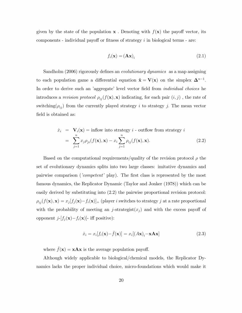
given by the state of the population x . Denoting with f(x) the payo¤ vector, its

components - individual payo¤ or �tness of strategy i in biological terms - are:

fi(x) = (Ax)i (2.1)

Sandholm (2006) rigorously de�nes an evolutionary dynamics as a map assigning

to each population game a di¤erential equation _x = V(x) on the simplex �n�1:

In order to derive such an �aggregate�level vector �eld from individual choices he

introduces a revision protocol �ij(f(x);x) indicating, for each pair (i; j) , the rate of

switching(�ij) from the currently played strategy i to strategy j: The mean vector

�eld is obtained as:

_xi = Vi(x) = in�ow into strategy i - out�ow from strategy i

=nXj=1

xj�ji(f(x);x)� xinXj=1

�ij(f(x);x): (2.2)

Based on the computational requirements/quality of the revision protocol � the

set of evolutionary dynamics splits into two large classes: imitative dynamics and

pairwise comparison (�competent� play). The �rst class is represented by the most

famous dynamics, the Replicator Dynamic (Taylor and Jonker (1978)) which can be

easily derived by substituting into (2.2) the pairwise proportional revision protocol:

�ij(f(x);x) = xj[fj(x)�fi(x)]+ (player i switches to strategy j at a rate proportional

with the probability of meeting an j-strategist(xj) and with the excess payo¤ of

opponent j-[fj(x)�fi(x)]- i¤ positive):

_xi = xi[fi(x)� �f(x)] = xi[(Ax)i�xAx] (2.3)

where �f(x) = xAx is the average population payo¤.

Although widely applicable to biological/chemical models, the Replicator Dy-

namics lacks the proper individual choice, micro-foundations which would make it

20

attractive for modelling humans interactions. The alternative - Best Response dy-

namic - already introduced by Gilboa andMatsui (1991) requires extra computational

abilities from agents, beyond merely sampling randomly a player and observing the

di¤erence in payo¤: speci�cally being able to compute a best reply strategy to the

current population state:

_xi = BR(x)� xi (2.4)

where,

BR(x) = argmaxyyf(x)

2.2.2 Discrete choice models-the Logit choice rule

Apart from the highly unrealistic assumptions regarding agents capacity to compute

a perfect best reply to a given population state there is also the drawback that (2.4)

de�nes a di¤erential inclusion, i.e. a set-valued function. The best responses may not

be unique and multiple trajectory paths can emerge from the same initial conditions.

A �smoothed�approximation of the Best Reply dynamics - the Logit dynamics -

was introduced by Fudenberg and Levine (1998); it was obtained by stochastically

perturbing the payo¤ vector f(x) and deriving the Logit revision protocol:

�ij(f(x);x) =exp[��1fj(x)]Pk exp[�

�1fk(x)]=

exp[��1Ax)i]Pk exp[�

�1Ax)k]; (2.5)

where � > 0 is the noise level. Here �ij represents the probability of player i

switching to strategy j when provided with a revision opportunity. For high levels

of noise the choice is fully random (no optimization) while for � close to zero the

switching probability is almost one. This revision protocol can be explicitly de-

rived from a random utility model or discrete choice theory (McFadden (1981), An-

derson et al. (1992)) by adding to the payo¤ vector f(x) a noise vector " with

a particular distribution, i.e. "i are i.i.d following the extreme value distribution

G("i) = exp(� exp(��1"i � )); = 0:5772 ( the Euler constant). The density of

21

this Weibull type distribution is

g("i) = G0("i) = �

�1 exp(��1"i � ) exp(� exp(��1"i � )):

With noisy payo¤s, the probability that strategy Ei is a best response can be

computed as follows:

P (i = argmaxj

h(Ax)j + "j

i) = P [(Ax)i + "i > (Ax)j + "j];8j 6= i

= P ["j < (Ax)i + "i � (Ax)j]j 6=i =1Z

�1

g("i)Yj 6=i

G((Ax)i + "i � (Ax)j)d"i

=

1Z�1

��1 exp(��1"i � )e(� exp(��1"i� ))

Yj 6=i

e(� exp(��1[(Ax)i+"i�(Ax)j ]� ))d"i

which simpli�es to our logit probability of revision:

�ij =exp[��1Ax)i]Pk exp[�

�1Ax)k]

An alternative way to obtain (2.5) is to deterministically perturb the set-valued

best reply correspondence (2.4) with a strictly concave function V (y) (Hofbauer

(2000)):

BR�(x) = arg maxy2�n�1

[y � (Ax) + V�(y)]

For a particular choice of the perturbation function V�(y) = �Pi=1;n

yi log yi; y 2�n�1

the resulting objective function is single-valued and smooth; the �rst order condition

yields the unique logit choice rule:

BR�(x)i =exp[��1Ax)i]Pk exp[�

�1Ax)k]

Plugging the Logit revision protocol (2.5) back into the general form of the mean

�eld dynamic (2.2) and making the substitution � = ��1 we obtain a well-behaved

22

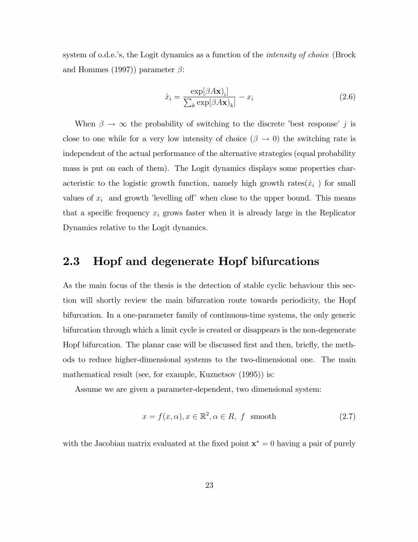
system of o.d.e.�s, the Logit dynamics as a function of the intensity of choice (Brock

and Hommes (1997)) parameter �:

_xi =exp[�Ax)i]Pk exp[�Ax)k]

� xi (2.6)

When � ! 1 the probability of switching to the discrete �best response� j is

close to one while for a very low intensity of choice (� ! 0) the switching rate is

independent of the actual performance of the alternative strategies (equal probability

mass is put on each of them). The Logit dynamics displays some properties char-

acteristic to the logistic growth function, namely high growth rates( _xi ) for small

values of xi and growth �levelling o¤�when close to the upper bound. This means

that a speci�c frequency xi grows faster when it is already large in the Replicator

Dynamics relative to the Logit dynamics.

2.3 Hopf and degenerate Hopf bifurcations

As the main focus of the thesis is the detection of stable cyclic behaviour this sec-

tion will shortly review the main bifurcation route towards periodicity, the Hopf

bifurcation. In a one-parameter family of continuous-time systems, the only generic

bifurcation through which a limit cycle is created or disappears is the non-degenerate

Hopf bifurcation. The planar case will be discussed �rst and then, brie�y, the meth-

ods to reduce higher-dimensional systems to the two-dimensional one. The main

mathematical result (see, for example, Kuznetsov (1995)) is:

Assume we are given a parameter-dependent, two dimensional system:

x = f(x; �); x 2 R2; � 2 R; f smooth (2.7)

with the Jacobian matrix evaluated at the �xed point x� = 0 having a pair of purely

23

imaginary, complex conjugates eigenvalues:

�1;2 = �(�)� i!(�); �(�) < 0; � < 0; �(0) = 0

and �(�) > 0; � > 0:

If , in addition, the following genericity2 conditions are satis�ed:

(i)h@�(�)@�

i�=0

6= 0 - transversality condition

(ii) l1(0) 6= 0, where l1(0) is the �rst Lyapunov coe¢ cient3 - nondegeneracy

condition,

then the system (2.7) undergoes a Hopf bifurcation at � = 0: As � increases the

steady state changes stability from a stable focus into an unstable focus.

There are two types of Hopf bifurcation, depending on the sign of the �rst Lya-

punov coe¢ cient l1(0) :

(a) If l1(0) < 0 then the Hopf bifurcation is supercritical : the stable focus x

becomes unstable for � > 0 and is surrounded by an isolated, stable closed orbit

(limit cycle).

(b)If l1(0) > 0 then the Hopf bifurcation is subcritical : for � < 0 the basin of

attraction of the stable focus x� is surrounded by an unstable cycle which shrinks

and disappears as � crosses the critical value � = 0 while the system diverges quickly

from the neighbourhood of x�.

In the �rst case the stable cycle is created immediately after � reaches the crit-

ical value and thus the Hopf bifurcation is called supercritical, while in the latter

the unstable cycle already exists before the critical value, i.e. a subcritical Hopf

bifurcation (Kuznetsov (1995)). The supercritical Hopf is also known as a soft or

2Genericity usually refer to transversality and non-degeneracy conditions. Rougly speaking,the transversality condition means that eigenvalues cross the real line at non-zero speed. Thenondegeneracy condition implies non-zero higher-order coe¢ cients in equation (2.10) below. Itensures that the singularity x� is typical (i.e. �nondegenerate�) for a class of singularities satisfyingcertain bifurcation conditions (see Kuznetsov (1995)).

3This is the coe¢ cient of the third order term in the normal form of the Hopf bifurcation (seeequation (2.10) below).

24

non-catastrophic bifurcation because , even when the system becomes unstable, it

still lingers within a small neighbourhood of the equilibrium bounded by the limit

cycle, while the subcritical case is a sharp/catastrophic one as the system now moves

quickly far away from the unstable equilibrium.

If l1(0) = 0 then there is a degeneracy in the third order terms of normal form

and , if other, higher order nondegeneracy conditions hold(i.e. non-vanishing second

Lyapunov coe¢ cient) then the bifurcation is called Bautin or generalized Hopf bi-

furcation. This happens when the �rst Lyapunov coe¢ cient vanishes at the given

equilibrium x� but the following higher-order genericity4 conditions hold:

(i) l2(0) 6= 0, where l2(0) is the second Lyapunov coe¢ cient - nondegeneracy

condition

(ii) the map �! (�(�); l1(�)) is regular (i.e. the Jacobian matrix is nonsingular)

at the critical value � = 0 - transversality condition.

Depending on the sign of l2(0), at the Bautin point the system may display a

limit cycle bifurcating into two or more cycles , coexistence of stable and unstable

cycles which collide and disappear, together with cycle blow-up.

Computation of the �rst Lyapunov coe¢ cient

For the planar case, l1(0) can be computed without explicitly deriving the normal

form, from the Taylor coe¢ cients of a transformed version of the original vector �eld.

The computation of l1(0) for higher dimensional systems makes use of the Center

Manifold Theorem by which the orbit structure of the original system near (x�; �0)

is fully determined by its restriction to the two-dimensional center manifold5. On

4Technically, these �higher-order�genericity conditions ensure that there are smooth invertiblecoordinate transformations, depending smoothly on parameters, together with parameter changesand (possibly) time re-parametrizations such that (2.7) can be reduced to a �simplest� form, thenormal form. See Kuznetsov (1995) pp. 309 for more details on the Bautin (generalized Hopf)bifurcation and for an expression for the second Lyapunov coe¢ cient l2(0):

5The center manifold is the manifold spanned by the eigenvectors corresponding to the eigen-values with zero real part.

25

the center manifold (2.7) takes the form (Wiggins (2003)):

0@ _x

_y

1A =

0@ Re�(�) � Im�(�)

Im�(�) Re�(�)

1A0@ x

y

1A+0@ f 1(x; y; �)

f 2(x; y; �)

1A (2.8)

where �(�) is an eigenvalue of the linearized vector �eld around the steady state and

f1(x; y; �); f2(x; y; �) are nonlinear functions of order O(jxj2) to be obtained from the

original vector �eld. Wiggins (2003) also provides a procedure for transforming (2.7)

into (2.8). Speci�cally, for any vector �eld _x = F (x); x 2 R2 let DF (x�) denote the

Jacobian evaluated at the �xed point x�.Then _x = F (x) is equivalent to:

_x = Jx+ T�1 �F (Tx) (2.9)

with J stands for the real Jordan canonical form of DF (x�); T is the matrix trans-

forming DF (x�) into the Jordan form, and �F (x) = F (x)�DF (x�)x: At the Hopf bi-

furcation point �0; �1;2 = �i! and the �rst Lyapunov coe¢ cient is (Wiggins (2003)):

l1(�) =1

16[f 1xxx+f

1xyy+f

2xxy+f

2yyy]+ (2.10)

+1

16![f 1xy(f

1xx+f

1yy)� f

2xy(f

2xx+f

2yy)� f

1xxf

2xx+f

1yyf

2yy] (2.11)

2.4 Three strategy games

We consider two well-known three-strategy games: the generalized Rock-Scissors-

Paper and the Coordination Game. In subsection (2.4.1) we �rst perform a local bi-

furcation analysis for a classical example of three-strategy games, the Rock-Scissors-

Paper. Two types of evolutionary dynamics - Replicator and Logit Dynamics - are

considered while the qualitative change in their orbital structure is studied with

respect to the behavioural parameter (�) and the payo¤ ("; �) parameters. In sub-

section (2.4.2) we provide numerical evidence for a sequence of fold bifurcations in

26

the Coordination game under the Logit Dynamics and depict the fold curves in the

parameter space.

2.4.1 Rock-Scissors-Paper Games

The Rock-Paper-Scissors class of games (or games of cyclical dominance) formalize

strategic interactions where each strategy Ei is an unique best response to strategy

Ei+1 for i = 1; 2 and E3 is a best rsponse to E16:

A =

0BBB@ 1 �2 "3

"1 2 �3

�1 "2 3

1CCCA ; �i � i � "i (2.12)

Due to the invariance under positive linear transformations of the payo¤ matrix

(2.12) (Zeeman (1980), Weissing (1991)) the main diagonal element can be set to

zero, by, for instance, substracting the diagonal entry from each column entries7:

A =

0BBB@0 �2 �"3�"1 0 �3

�1 �"2 0

1CCCA ; �i; "i � 0 (2.13)

If matrix (2.13) is circulant (i.e. �i = �; "i = "; i = 1; 2; 3) then the RSP game is

called circulant, while for a non-circulant matrix (2.13) we have a generalized RSP

game. The behavior of Replicator and Logit Dynamics on the class of circulant RSP

games will be investigated, both analytically and numerically, in the �rst and second

part of this subsection, respectively. Numerical results about the generalized RSP

class of games under Logit Dynamics are reported in the third part.

6see Weissing (1991) for a thourough charaterization of the discrete-time Replicator Dynamicsbehavior on this class of games.

7We stick to the same notations as in (2.12) although it is apparent that the new �0s and "0sare di¤erent from the old ones as they are derived via the above mentioned linear transformation.

27

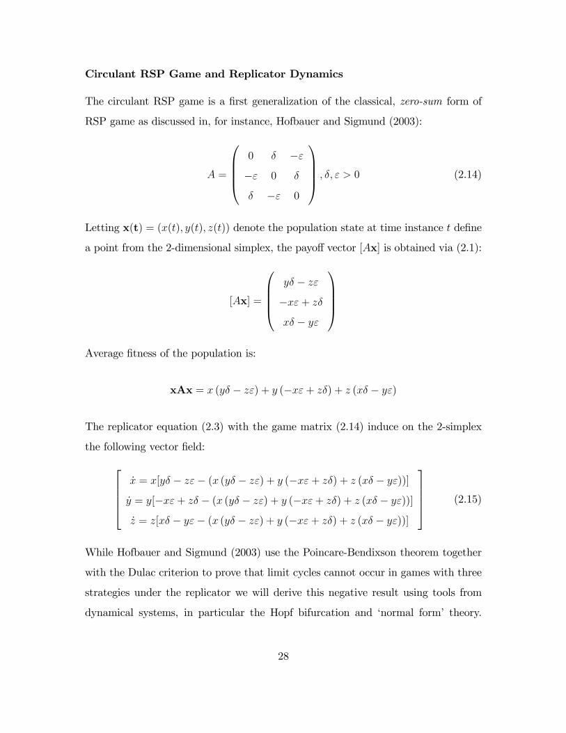
Circulant RSP Game and Replicator Dynamics

The circulant RSP game is a �rst generalization of the classical, zero-sum form of

RSP game as discussed in, for instance, Hofbauer and Sigmund (2003):

A =

0BBB@0 � �"

�" 0 �

� �" 0

1CCCA ; �; " > 0 (2.14)

Letting x(t) = (x(t); y(t); z(t)) denote the population state at time instance t de�ne

a point from the 2-dimensional simplex, the payo¤ vector [Ax] is obtained via (2.1):

[Ax] =

0BBB@y� � z"

�x"+ z�

x� � y"

1CCCAAverage �tness of the population is:

xAx = x (y� � z") + y (�x"+ z�) + z (x� � y")

The replicator equation (2.3) with the game matrix (2.14) induce on the 2-simplex

the following vector �eld:26664_x = x[y� � z"� (x (y� � z") + y (�x"+ z�) + z (x� � y"))]

_y = y[�x"+ z� � (x (y� � z") + y (�x"+ z�) + z (x� � y"))]

_z = z[x� � y"� (x (y� � z") + y (�x"+ z�) + z (x� � y"))]

37775 (2.15)

While Hofbauer and Sigmund (2003) use the Poincare-Bendixson theorem together

with the Dulac criterion to prove that limit cycles cannot occur in games with three

strategies under the replicator we will derive this negative result using tools from

dynamical systems, in particular the Hopf bifurcation and �normal form� theory.

28

The same toolkit will be applied next to the Logit Dynamic and a positive result -

stable limit cycles do occur - will be derived.

As we are interested in limit cycles within the simplex we consider only in-

terior �xed points of this system (any replicator dynamic has the simplex ver-

tices as steady states, too). For the parameter range "; � > 0 the barycentrum

x� = [x = 1=3; y = 1=3; z = 1=3] is always an interior �xed point of (2.15). In order

to analyze its stability properties we obtain �rst, by substituting z = 1� x� y into

(2.15), a proper 2 dimensional dynamical system of the form:

24 _x

_y

35 =24 �x"+ 2xy"� x2� + 2x2"+ x3� � x3"+ xy2� + x2y� � xy2"� x2y"

y� � 2xy� � 2y2� + y2"+ y3� � y3"+ xy2� + x2y� � xy2"� x2y"

35(2.16)

We can detect the Hopf bifurcation threshold at the point where the trace of the Jac-

obian matrix of (2.16) is equal to zero. The Jacobian evaluated at the barycentrical

steady state x� is

24 " � + "

�� " ��

35, with eigenvalues: �1;2("; �) = 12(" � �) � i

p32

p("+ �)2 and trace " � �: For � < "; x� is an unstable focus, at � = " a pair

of imaginary eigenvalues crosses the imaginary axis(�1;2 = �ip3�), while for � > "

x� becomes a stable focus (see Fig. (2.1) below). This is consistent with Theorem

6 in Zeeman (1980) which states that the determinant of the matrix A determines

the stability properties of the interior �xed point. In example (2.14) DetA = "3� �3

vanishes for " = �: By the same Theorem 6 in Zeeman (1980) the vector �eld (2.15)

has a center in the 2-simplex and a continuum of cycles if DetA = 0:

Alternatively, our local bifurcation analysis suggests that a Hopf bifurcation oc-

curs when " = � and in order to ascertain its features - sub/supercritical or degenerate

- we have to further investigate the nonlinear vector �eld near the (x�; " = �) point.

At the Hopf bifurcation " = � necessary condition Re�1;2("; �) = 0; vector �eld (2.16)

29

takes a simpler form: 24 _x

_y

35 =24 �x� + 2xy� + x2�y� � 2xy� � y2�

35Using formula (2.8) we can back out the nonlinear functions f 1; f2 needed for the

computation of the �rst Lyapunov coe¢ cient:24 f1(x; y) = yp3� � x� + 2xy� + x2�

f2(x; y) = �xp3� + y� � 2xy� � y2�

35We can now state the following result:

Lemma 1 All Hopf bifurcations are degenerate in the circulant Rock-Scissor-Paper

game under Replicator Dynamics.

Proof. From the nonlinear functions f1(x; y); f2(x; y) derived above we can easily

compute the �rst Lyapunov coe¢ cient (2.10) as l1("Hopf = �Hopf ) = 0 which means

that there is a �rst degeneracy in the third order terms from the Taylor expansion of

the normal form. The detected bifurcation is a Bautin or degenerate Hopf bifurcation

( assuming away other higher order degeneracies: technically, the second Lyapunov

coe¢ cient l1("Hopf = �Hopf ) should not vanish).

Although, in general, the orbital structure at a degenerate Hopf bifurcation may

be extremely complicated (see Section (2.3)), for our particular vector �eld induced

by the Replicator Dynamics it can be shown by Lyapunov function techniques (Hof-

bauer and Sigmund (2003), Zeeman (1980)) that a continuum of cycles is born exactly

at the critical parameter value8.

8The absence of a generic Hopf bifurcation does not su¢ ce to conclude that the vector �eldadmits no isolated periodic orbits and �global� results are required (e.g. the Bendixson-Dulacmethod, positive divergence of the vector �eld on the simplex).

30

0 0.2 0.4 0.6 0.8 1

0.2

0.4

0.6

0.8

1

x

y

(a) Unstable focus,

� = 0:6; " = 1

0 0.2 0.4 0.6 0.8 1

0.2

0.4

0.6

0.8

1

x

y

(b) Degenerate Hopf,

� = 1; " = 1

0 0.2 0.4 0.6 0.8 1

0.2

0.4

0.6

0.8

1

x

y

(c) Stable focus,

� = 1:1; " = 1

Figure 2.1: Rock-Scissors-Paper and Replicator Dynamics for �xed " = 1 and varying �.Qualitative changes in the phase portraits - unstable focus (Panel (a)), continuum of cycles(Panel (b)) and stable focus (Panel (c)) - occur as we increase � from below to above ".

It would be worth pointing out the connection between our local (in)stability res-

ults and the static concept of Evolutionary Stable Strategy (ESS). As already noted

in the literature (Zeeman (1980), Hofbauer (2000)) ESS implies (global) asymptotic

stability under a wide class of evolutionary dynamics - Replicator Dynamics, Best

Response and Smooth Best Response Dynamics, Brown-von Newmann-Nash, etc.

The reverse implication does not hold in general, i.e. the local stability analysis does

not su¢ ce to qualify an attractor as an ESS. However, for � < " we have shown that

x� is an unstable focus and we can conclude that, for this class of RSP games, the

barycentrum is not an ESS. Indeed, the case � < " is the so called bad RSP game

(Sandholm (2008)) which is known not to have an ESS. For � > " we are in the good

RSP game and it does have an interior ESS which coincides with the asymptotically

stable rest point x� of the Replicator Dynamics. Last, if � = " (i.e. standard RSP)

then x� is a neutrally stable strategy/state and we proved that in this zero-sum

game the Replicator undergoes a degenerate Hopf bifurcation. The Hopf bifurcation

scenario is illustrated in Fig. 2.1 for a particular value of ":

31

Circulant RSP Game and Logit Dynamics

The logit evolutionary dynamics (2.6) applied to our normal form game (2.14) leads

to the following vector �eld:26664_x = exp(�(y��z"))

exp(�(y��z"))+exp(�(�x"+z�))+exp(�(x��y")) � x

_y = exp(�(�x"+z�))exp(�(y��z"))+exp(�(�x"+z�))+exp(�(x��y")) � y

_z = exp(�(x��y"))exp(�(y��z"))+exp(�(�x"+z�))+exp(�(x��y")) � z

37775 (2.17)

By substituting z = 1 � x � y into (2.17) we can reduce the initial system to a

2-dimensional system of equations and solve for its �xed points in the interior of the

simplex, numerically, for di¤erent parameters values (�; "; �):

24 exp(�(y��"(�x�y+1)))exp(�(x��y"))+exp(�(�x"+�(�x�y+1)))+exp(�(y��"(�x�y+1))) � x = 0

exp(�(�x"+�(�x�y+1)))exp(�(x��y"))+exp(�(�x"+�(�x�y+1)))+exp(�(y��"(�x�y+1))) � y = 0

35 (2.18)

The 2 � dim simplex barycentrum [x = 1=3; y = 1=3; z = 1=3] remains a �xed

point irrespective of the value of �. The Jacobian of (2.18) evaluated at this steady

state is:

24 13�"� 1 1

3�� + 1

3�"

�13�� 1

3�" �1

3�� 1

35 ; with eigenvalues: �1;2 = 16�" � 1

6�� 1 �

i12

q13(�� + �"):The Hopf bifurcation (necessary) condition Re(�1;2) = 0 leads to:

�Hopf =6

"� � ; 0 < � < " (2.19)

We notice that for the zero-sum RSP game (" = �) - unlike Replicator Dynamics

which exhibited a degenerate Hopf at " = � - the barycentrum is always asymptot-

ically stable (Re�1;2 = �1) under Logit Dynamics. We have the following:

Lemma 2 The Logit Dynamics (2.17) on the circulant Rock-Scissors-Paper game

exhibits a generic Hopf bifurcation and, therefore, has limit cycles. Moreover, all

such Hopf bifurcations are supercritical, i.e. the limit cycles are born stable.

32

Proof. Condition (2.19) gives the necessary �rst-order condition for Hopf bi-

furcation to occur ; in order to show that the Hopf bifurcation is non-degenerate we

have to compute, according to (2.10) the �rst Lyapunov coe¢ cient l1(�Hopf ; "; �) and

check whether it is non-zero. The analytical form of this coe¢ cient takes a complic-

ated expression of exponential terms (see appendix (2.A)) which, after some tedious

computations, boils down to:

l1(�Hopf ; "; �) = �864(�"+ �

2 + "2)

3(3"� 3�)2 < 0; " > � > 0:

Computer simulations of this route to a stable cycle are shown in Fig. 2.2 below.

We notice that as � moves up from 10 to 35 (i.e. the noise level is decreasing)

the interior stable steady state looses stability via a supercritical Hopf bifurcation

and a small, stable limit cycle emerges around the unstable steady state. Unlike

Replicator Dynamics, stable cyclic behavior does occur under the Logit dynamics

even for three-strategy games.

0 0.2 0.4 0.6 0.8 1

0.2

0.4

0.6

0.8

1

x

y

(a) Stable focus, � = 10

0 0.2 0.4 0.6 0.8 1

0.2

0.4

0.6

0.8

1

x

y

(b) Generic Hopf, � = 30

0 0.2 0.4 0.6 0.8 1

0.2

0.4

0.6

0.8

1

x

y

(c) Limit cycle, � = 35

Figure 2.2: Rock-Scissors-Paper and Logit Dynamics for �xed game " = 1; � = 0:8 andfree behavioral parameter �. Qualitative changes in the phase portraits: a stable interior�xed point (Panel (a)) loses stability when the critical threshold � = 30 is hit, via a generic,supercritical Hopf bifurcation (Panel (b)) and, if � is pushed up even further, a stable limitcycle is born (Panel (c)).

33

Similar periodic behaviour can be detected in the payo¤ parameter space as in

Fig. 2.3 below where the noise level is kept constant and the game is allowed to

change.

0 0.2 0.4 0.6 0.8 1

0.2

0.4

0.6

0.8

1

x

y

(a) Stable focus, � = 1

0 0.2 0.4 0.6 0.8 1

0.2

0.4

0.6

0.8

1

x

y

(b) Hopf, � = 0:399

0 0.2 0.4 0.6 0.8 1

0.2

0.4

0.6

0.8

1

x

y

(c) Limit cycle, � = 0:1

Figure 2.3: Rock-Scissors-Paper and Logit Dynamics for �xed behavioral parameter � =10 and free game parameter � [" = 1]. Qualitative changes in the phase portraits: a stableinterior �xed point (Panel (a)) loses stability when the critical threshold � = 0:399 is hit,via a generic, supercritical Hopf bifurcation (Panel (b)). Panel (c) display a stable limitcycle for � = 0:1 that attracts trajectories originating both outside and inside the cycle.

A more thorough search in the parameters space is performed with the help

of a sophisticated continuation software9(Dhooge et al. (2003)) which enable us to

determine all combination of relevant parameters giving rise to a speci�c singularity.

Figure 2.4 depicts curves of Hopf bifurcations in the (�; ") and (�; �) parameter space

(�xing �(") to 1). As we cross these Hopf curves from below the stable interior �xed

point loses stability and a stable periodic attractor surrounds it.

9MatCont (see package documentation at http://sourceforge.net/projects/matcont/).

34

0 0.2 0.4 0.6 0.8 1

20

40

60

6

δ

β

H

Hstablef ocus

stablelimit cy cle

(a) " = 1: Hopf curve � � �

0 2 4 6 8 101

20

40

60

ε

β

H

stablelimit cycle

stablefocus

H

(b) � = 1: Hopf curve � � "

Figure 2.4: Rock-Scissors-Paper and Logit Dynamics: Supercritical Hopf curves in (�; �)and (�; ") parameter spaces. Continuation of a detected co-dimension I singularity (i.e.Hopf bifurcation) with respect to a second parameter gives rise to curves of supercriticalHopf points in the circulant RSP class of games.

Generalized RSP Game and Logit Dynamics

In this subsection we discuss the occurrence of limit cycles in the most general spe-

ci�cation of a Rock-Scissors-Paper game (2.13) under Logit Dynamics. For circulant

RSP game (i.e.circulant payo¤matrix) Weissing (1991) proved that the discrete and

continuous time Replicator Dynamics are �qualitatively�equivalent. However, for a

non-circulant payo¤ matrix (2.20), co-existing stable and unstable limit cycles are

found under discrete-time Replicator Dynamics. This sharply contrasts with the be-

haviour of the continuous-time Replicator Dynamics which is known not to give rise

to generic Hopf bifurcations. On the other hand, as shown in the previous subsec-

tion stable limit cycles do occur under Logit Dynamics so a natural question to pose

is whether multiple, interior periodic attractors can be detected under the logistic

dynamics in the generalized version of the circulant RSP game.

Weissing (1991) presents the following generalized RSP game as an example of

co-existing limit cycles under discrete-time Replicator Dynamics:

35

W =

0BBB@k b1 d1

d2 k b2

b1 + 3� d1 � 3� k

1CCCA ; bi > k � di; d1 � 3� > 0 (2.20)

We have already seen that this general speci�cation can be turned into (2.13)

by a positive linear payo¤ transformations as the continuous-time dynamics remain

invariant under such transformation10.

In the sequel we will investigate, numerically, the dynamical system resulting from

the generalized game payo¤ matrix (2.13) and the Logit evolutionary dynamics:

_xi =e�(Ax)i

3Pi=1

e�(Ax)i

;Ax =

26664�2x2 � "3x3�3x3 � "1x1�1x1 � "2x2

37775Figure 2.5 displays typical curves of fold and Hopf bifurcations produced by

MatCont, along with their codimension II singularities in various sub-regions of the

parameters space. The curves are initiated at certain bifurcation points11 detected

along the system�s equilibria curves. They �rst generalize results obtained in previ-

ous subsection for a circulant RSP payo¤ matrix to the entire class of RSP games.

Second, from the bifurcation diagrams we can detect, the co-existence of multiple

interior steady-states (born via Limit Point bifurcation) and limit cycle (created

when a Hopf curve is crossed). However, the fold curves seem to emerge beyond the

generalized RSP class of games (i.e. the positive R2 orthant in each 2-parameter

subspace)

In order to address the question of co-existing limit cycles under continuous-time

10For continous-time Replicator Dynamics the proof could be found in Weissing (1991)). Yet,the dynamics on (2.20 ) and (2.13) may be qualitatively di¤erent under discrete-time version of theReplicator Dynamics.11A supercritical (�rst Lyapunov coe¢ cient l1 = �3:222) Hopf point is detected at �1 = 0:626

and two Fold points at �1 = �0:554 and �1 = �0:952. Benchmark parameterization: � = 8:3; �1 =4; �2 = 3; �3 = 2; "1 = 2; "21 = 3; "3 = 4:

36

Logit Dynamics, one should run a systematic search in the parameter space for a

fold bifurcation of limit cycles: detect the Hopf points, continue them with respect to

each of the 6-parameter in the game form (2.13) and, then track any codimension II

singularity (most interestingly, the limit point of cycles bifurcation). A representative

subset of the resulting Hopf curves is plotted in Fig. 2.5. Except for the Bogdanov-

Takens (BT) bifurcation, no further codimension II singularities are detected by the

continuation package in the positive R2 orthant corresponding to the generalized

class of RSP game. In particular, there is no limit point/fold bifurcation of cycles,

i.e. multiple, co-existing (un)stable limit cycles are ruled out.

37

5 2 1 4 7 10

2

1

4

7

10

δ2

δ 1

CP

ZH

HLP

LP

LP H

5 2 1 4 7 10

2

1

4

7

10

δ3

δ 1

ZH

CP

LP

H

H

LPLP

1 2 3 42

1

0

1

2

3

4

ε1

δ 1

ZHCPBTLPH

LP

H

0 2 4 6 8 10

2

4

6

8

10

ε3

ε 1CP

BT

ZH

LPLP

LP

LP

H

H

5 10 1521

1

3

5

7

9

β

ε 3

CP

ZH

ZH

CP

LPLPH

LP

LP

H

2 4 6 8 10 12

1

0.5

0

0.5

1

β

δ 1

ZHCP BT

H

HLP

LP

Figure 2.5: Generalized Rock-Scissors-Paper - curves of codimension I - fold (LP) andHopf (H) - bifurcations along with the detected codimension II singularities - Cusp (CP),Bogdanov-Taken (BT), Cusp (CP) and Zero-Hopf (ZH) points - in various two-parametersubspaces. Unless free to �oat, game parameters are �xed to following values - �1 =0:62; �2 = 4; �3 = 3; "1 = 2; "2 = 3; "3 = 4 - while the intensity of choice is � = 8

38

2.4.2 Coordination Game

Using topological arguments, Zeeman (1980) shows that three-strategies games have

at most one interior, isolated �xed point under Replicator Dynamics ( see The-

orem 3 in Zeeman (1980)). In particular, fold catastrophe (two isolated �xed points

which collide and disappear when some parameter is varied) cannot occur within the

simplex. In this section we provide - by means of the classical coordination game -

numerical evidence for the occurrence of multiple, isolated interior steady-states un-

der the Logit Dynamics and show that fold catastrophe is possible when we alter the

intensity of choice �. The coordination game we consider is given by the following

payo¤ matrix:

A =

0BBB@1� " 0 0

0 1 0

0 0 1 + "

1CCCA ; " 2 (0; 1)Coordination Game and Replicator Dynamics

The vector �eld _x = x[Ax� xAx] becomes:

26664_x = x[x (�"+ 1)� (y2 + z2 ("+ 1) + x2 (�"+ 1))]

_y = y[y � (y2 + z2 ("+ 1) + x2 (�"+ 1))]

_z = z[z ("+ 1)� (y2 + z2 ("+ 1) + x2 (�"+ 1))]

37775 (2.21)

This systems has the following �xed points in simplex coordinates:

(i) simplex vertices (stable nodes): (1; 0; 0); (0; 1; 0); (0; 0; 1)

(ii) interior (source): O ( "+13�"2 ;

1�"23�"2 ;

1�"3�"2 )

(iii) on the boundary (saddles):

M ( 12�" ;

1�"2�" ; 0); N ( 1

2�" ; 0;1�"2�"); P (0;

12�" ;

1�"2�")

The eigenvalues of the corresponding Jacobian evaluated at each of the above

�xed points are:

A [x = 0; y = 1; z = 0] ; eigenvalues: �1;2;3 = �1

39

B [x = 1; y = 0; z = 0]; eigenvalues: �1;2;3 = "� 1

C [x = 0; y = 0; z = 1]; eigenvalues: �1;2;3 = �"� 1

O [x = "+13�"2 ; y =

1�"23�"2 ; z =

1�"3�"2 ]; eigenvalues: �1;2 =

"2�1"2�3 > 0; for " 2 (0; 1)

M [x = 12�" ; y =

1�"2�" ; z = 0]; eigenvalues: �1;2 = �

1�""�2

N [x = 12�" ; y = 0; z =

1�"2�" ]; eigenvalues: �1;2 = �

1�4"+"2+4 (2"+ "

2 � "3 � 2)

P [x = 0; y = 12�" ; z =

1�"2�" ]; eigenvalues: �1;2 = �

1�4"+"2+4 ("+ "

2 � "3 � 2)

This �xed points structure is consistent with Zeeman (1980) result that no fold

catastrophes (i.e. multiple, isolated and interior steady states) can occur under the

Replicator Dynamics. The three saddles together with the interior source de�ne the

basins of attractions for the simplex vertices. The boundaries of the simplex are

invariant under Replicator Dynamics12 and it su¢ ces to show that the segment lines

[OM ]; [ON ], and [OP ] ( see Fig. 2.6 for a plot of these segments for " = 0:1) are

also invariant under this dynamics.

A (1,0,0)B (0,1,0)C (0,0,1)

O

B P C

M N

A

Figure 2.6: Coordination Game with " = 0:1 and Replicator Dynamics - Invariant mani-folds

12see proof in Hofbauer and Sigmund (2003) pp. 67-68.

40

Lemma 3 The segment lines [OM ]; [ON ], and [OP ] are invariant under Replicator

Dynamics and they form, along with the simplex edges, the boundaries of the basins

of attraction for the three stable steady states.

Proof. Using the standard substitution z = 1� x� y system (2.21) becomes:

24 _x = x2 � x3 � xy2 � x2"+ x3"� x (�x� y + 1)2 � x" (�x� y + 1)2

_y = y2 � y3 � x2y + x2y"� y (�x� y + 1)2 � y" (�x� y + 1)2

35 (2.22)

Segment [MO] is de�ned, in simplex coordinates, by y = x(1 � "). Along this line

we have:

�_y

_x

�[MO]:y=x(1�")

=x (�"+ 1)

�x (�"+ 1)� x2 (�"+ 1)� x2 (�"+ 1)2 � ("+ 1) (�x� y + 1)2

�x�x (�"+ 1)� x2 (�"+ 1)� x2 (�"+ 1)2 � ("+ 1) (�x� y + 1)2

�= 1� ";

which is exactly the slope of [MO]. Similarly, invariance results are obtained for

segments [ON ] and [OP ] de�ned by x(1� ") = z(1 + ") and y = z(1 + "):

Analytically, the basins of attraction are determined by the areas of the polygons

delineated by the invariant manifolds [OM ]; [ON ], and [OP ] and the 2-dim simplex

boundaries, as follows:

A(1; 0; 0) = A[AMON ] =

26664��18 p32�" � 1

4

p33�2"4�2" �

18

p3 "+13�"2 +

14

p3 3�"6�2"2 �

14

p3

2�"3�"6�2"2

��+��14p3 ("+ 1) 3�2"

(4�2")(3�"2) +18

p3

2�" �14

p3

4�2" �18

p3 "+13�"2

��+��14p3 3�"

6�2"2 +14

p3 "+1(4�2")(3�"2) �

14

p3

2�"3�"6�2"2

��

37775B(0; 1; 0) = A[BMOP ] =

��14p3 "+1(4�2")(3�"2) �

14

p3

2�"3�"6�2"2

��+��14p3 ("+ 1) 1�"(2�")(3�"2)

��C(0; 0; 1) = A[CNOP ] =

�� 14p3("+1)(1�")�(1+")(2�")(3�"2) � 14

p3 "+13�"2

��+��14p3 ("+ 1) 3�2"(4�2")(3�"2)

��The basins�sizes vary with the payo¤ perturbation parameter " as in Table 2.1.

When the payo¤asymmetries are small, the simplex of initial conditions is divided

equally among the three �xed points/equilibria (Fig. 2.7a). As the payo¤ discrepan-

cies increase most of the initial conditions are attracted by the welfare-maximizing

equilibrium (0; 0; 1) ( see Fig. 2.7b).

41

"nA A(1; 0; 0) B(0; 1; 0) C(0; 0; 1) Long-Run Average Fitness/Welfare0 33:33% 33:33% 33:33% 10:1 29:9% 33:2% 36:7% 1:00480:5 15:5% 30:3% 54:54% 1:19860:6 8:92% 12:18% 78:90% 1:419 90:9 1:2% 12% 86:7% 1:512

Table 2.1: Coordination Game, Replicator Dynamics�Long-run average �tness for di¤erentpayo¤-perturbation parameter "

0 0.2 0.4 0.6 0.8 1

0.2

0.4

0.6

0.8

1(1,0,0)29%(0,1,0)33.3%(0,0,1)37.7%

(a) A"[" = 0:1]

0 0.2 0.4 0.6 0.8 1

0.2

0.4

0.6

0.8

1(1,0,0)3%(0,1,0)34.4%(0,0,1)62.6%

(b) A"[" = 0:8]

Figure 2.7: Coordination Game and Replicator Dynamics-basins of attraction for di¤erentvalues of the payo¤ parameter "

Coordination Game and Logit Dynamics

We choose a small payo¤ perturbation, " = 0:1; such that system is �close�to the

symmetric basins of attraction A,B and C in the Replicator Dynamics. Logit Dy-

namics together with payo¤matrix A de�ne the following vector �eld on the simplex

of frequencies (x; y; z) of strategies E1; E2; E3, respectively:

42

26664_x = exp(0:9�x)

exp(0:9�x)+exp(�y)+exp(1:1�z)� x

_y = exp(�y)exp(0:9�x)+exp(�y)+exp(1:1�z)

� y

_z = exp(1:1�z)exp(0:9�x)+exp(�y)+exp(1:1�z)

� z

37775In order to ascertain the number of (asymptotically) stable �xed points on the

two-dimensional simplex we �rst run simulations for increasing values of � and for

di¤erent initial conditions within the simplex:

Case I. � � 0: One interior steady state (initial conditions, time series and at-

tracting point in Fig. 2.8a). The barycentrum is globally attracting, i.e. irrespective

of the initial proportions, the population will settle down to a state with equalized

fractions.

Case II. � � 10: Three stable steady states asymptotically approaching the ver-

tices of the simplex as � increases (Fig. 2.8b-d) plus other unstable steady states.

The size of their basins of attraction is determined both by the strategy relative

payo¤ advantage and by the value of the intensity of choice: Whichever of the three

strategy happens to outnumber the other two in the initial population, will eventually

win the evolutionary competition.

43

0 . 2

0 . 2 5

0 . 3

0 . 3 5

0 . 4

1 5 9 1 3 1 7 2 1

xyz

(a) � = 0, any initial mixture (x; y; z)

converges to (1=3; 1=3; 1=3)

0

0 . 2

0 . 4

0 . 6

0 . 8

1

1 5 9 1 3 1 7 2 1

xyz

(b) � = 10, initial mixture

(0:4; 0:3; 0:3)! (1; 0; 0)

0

0 . 2

0 . 4

0 . 6

0 . 8

1

1 5 9 1 3 1 7 2 1

xyz

(c) � = 10, initial mixture

(0:25; 0:4; 0:35)! (0; 1; 0)

0

0 . 2

0 . 4

0 . 6

0 . 8

1

0 4 8 1 2 1 6 2 0

xyz

(d) � = 10, initial fractions

(0:33; 0:33; 0:34)! (0; 0; 1)

Figure 2.8: Coordination Game[" = 0:1] and Logit Dynamics -Unique stable steady statefor � low (Panel(a)) and three, co-existing stable steady states for high � = 10 (Panels(b)-(d)).

Multiple Equilibria. The most interesting situations occur in transition from

high to low values of the behavioral parameter �: we will show that the Logit Dy-

namics undertakes a sequence of fold bifurcations by which each of the three stable

44

steady states collides with another unstable steady state from within the simplex

and disappears. Fig. 2.9cd shows simulations of time series converging to a unique

steady state for low values of � (� = 2:6): Panels (a)-(b) show the co-existence of two

steady-states for � = 3 as di¤erent initial population mixtures converge to di¤erent

steady states.

0

0 . 2

0 . 4

0 . 6

0 . 8

1

0 4 8 1 2 1 6 2 0

xyz

(a) � = 3, initial mixture

(0:2; 0:6; 0:2)! (0:1; 0:8; 0:1)

0

0 . 2

0 . 4

0 . 6

0 . 8

1

0 4 8 1 2 1 6 2 0

xyz

(b) � = 3, initial mixture

(0:5; 0:3; 0:2)! (0:06; 0:06; 0:88)

0

0 . 2

0 . 4

0 . 6

0 . 8

1

0 4 8 1 2 1 6 2 0 2 4 2 8

xyz

(c) � = 2:6, initial mixture

(0:8; 0:1; 0:1)! (0:11; 0:11; 0:78)

0

0 . 2

0 . 4

0 . 6

0 . 8

1

0 4 8 1 2 1 6 2 0 2 4 2 8

xyz

(d) � = 2:6, initial mixture

(0:4; 0:4; 0:1)! (0:11; 0:11; 0:78)

Figure 2.9: Coordination Game[" = 0:1] and Logit Dynamics with moderate level of noise-Panels (a)-(b) display two interior, isolated stable steady states, while Panels (c)-(d) showsconvergence to a unique, interior steady state

45

Bifurcations. Unlike Replicator, the Logit Dynamics displays multiple, interior

isolated steady states created via a fold bifurcation. In the particular case of a 3-

strategy Coordination game, three interior stable steady states emerge through a

sequence of two saddle-node bifurcations.

Fig. 2.10 depicts the fold bifurcations scenario by which the multiple, interior

�xed points appear when the intensity of choice (Panel (a)) or the payo¤ parameter

(Panel (b)) changes. For small values of � the unique, interior stable steady state

is the simplex barycentrum (1=3; 1=3; 1=3). As � increases this steady state moves

towards the Pareto-superior equilibrium (0; 0; 1). A �rst fold bifurcation occurs at

� = 2:77 and two new �xed points are created, one stable and one unstable. If

we increase � even further (� � 3:26) a second fold bifurcation takes place and two

additional equilibria emerge, one stable and one unstable. Last, two new �xed points

arise at � = 4:31 via a saddle-source bifurcation13. There is co-existence of three

stable steady states for large values of the intensity of choice �, the �logit equilibria�.

A similar sequence of bifurcations is visible in the payo¤parameter space (Fig. 2.10b)

where a family of fold bifurcations is obtained for a particular value of the switching

intensity �.

13At a saddle-source bifurcation two additional unstable steady states emerge.

46

2 2.7 3.2 4.3 6 70

0.2

0.4

0.6

0.8

1

β

x

LP

LP

LP

(a) Cascade of Fold bifurcations in

(x,�) space. "=0.1

0 0.2 0.4 0.6 0.8 10

0.2

0.4

0.6

0.8

1

ε

x

LP HH

HLP

LP

LP

H

H

LP

(b) Cascade of Fold bifurcations in (x,")

space. �=5.

Figure 2.10: Coordination Game and Logit Dynamics. Curves of equilibria along withcodimension I singularities, in this case fold (LP) points. Panel (a)-(b): the multiplicity ofsteady states arises through a sequence of three limit point(fold) bifurcations as one of thetwo parameters varies.

The continuation of the fold curves in the (�; ") parameter space allows the de-

tection of codimension II bifurcations. The cusp points in Fig. 2.11 below organize

the entire bifurcating scenario and capture the emergence of multiple, interior point-

attractors in Coordination Game under the smoothed best response dynamics. Once

such a curve of fold points is crossed from below two additional equilibria are created:

one stable and one unstable after a saddle-node bifurcation and two unstable steady

states after a saddle-source bifurcation. If choice is virtually random (� = 0) there

is an unique steady state while for large � there are 7 steady states (3 stable and 4

unstable).

47

0.4 0.2 0 0.2 0.42

4

6

8

ε

β

CP

ZH

ZH ZH

CP1

3

7

5

(a) Curves of fold points in the ("; �)

space

0.05 0.03 0.01 0.01 0.03 0.05

2.6

2.8

3

3.2

3.4

3.6

ε

β

ZH

CPCP

ZH

7

5

3

1

(b) Cusp points (CP) organize the

equilibria structure

Figure 2.11: Coordination Game and Logit Dynamics. Curves of fold points along withdetected codimension II singularities - in this case, cusp (CP) and zero-Hopf (ZH) points- traced in the ("; �) parameter space

Basins of Attraction. The numerical computation of the basins of attraction for

di¤erent equilibria reveals interesting properties of the Logit dynamics from a social

welfare perspective. We construct a measure of long-run aggregate welfare as the

payo¤ at the stable steady state weighted by its corresponding basin of attraction

size. While for extreme values of the intensity of choice the basins of attraction are

similar in size with the Replicator Dynamics (Panels (a), (c), (d) in Fig. 2.12,2.13),

for moderate levels of rationality the population manages to coordinate close to the

Pareto optimal Nash equilibria (Panel (b) in Fig. 2.12,2.13). The aggregate welfare

evolves non-monotonically with respect to the behavioural parameter � and, for

a given payo¤ perturbation "; it is maximal just before the �rst bifurcation occurs

�LP1 = 2:77:

48

(1/3,1/3,1/3)100%

(0,1,0)

(0,0,1)(0,1,0)

(1,0,0)

(a) � = 1;one barrycentrical steady

state

(0.13,0.14,0.73)100%

(1,0,0)(0,1,0)

(1,0,0)

(b) � = 10=4; one steady state �close�

to the Pareto superior equilibrium

(0.05,0.89,0.06)76.9%(0.03,0.03,0.94)23.1%

(0,1,0) (0,0,1)

(1,0,0)

(c) � = 10=3; two stable steady states

(1,0,0) 29%(0,1,0) 33.5%(0,0,1) 37.5%

(0,1,0) (0,0,1)

(1,0,0)

(d) � = 15; three stable steady

states

Figure 2.12: Coordination Game [" = 0:1] and Logit Dynamics: Panels (a)-(d), basins ofattraction for increasing values of the intensity of choice �. Fractions converging to eachof the steady state are indicated in the box

49

(1/3, 1/3, 1/3)100%

(0,1,0) (0,0,1)

(1,0,0)

(a) � = 0:5;unique, barrycentrical

steady state

(0.06,0.06,0.88)100%

(0,1,0) (0,0,1)

(1,0,0)

(b) � = 2;unique steady state, near

the Pareto superior equilibrium

(0.04,0.91,0.05)25%(0.001,0,0.999)75%

(0,1,0) (0,0,1)

(1,0,0)

(a) � = 4;two stable steady states

(1,0,0)5%(0,1,0)35%(0,0,1)60%

(0,0,1)(0,1,0)

(1,0,0)

(d) � = 15;three stable steady states

Figure 2.13: Coordination Game [" = 0:6] and Logit Dynamics: Panels (a)-(d), basins ofattraction for increasing values of the intensity of choice �

The long run average welfare evolves non-monotonically with respect to the be-

havioural parameter � (Fig. 2.14ab): it increases as the fully mixed equilibrium

slides slowly towards the Pareto optimal (0; 0; 1) vertex, attains a maximum before

the �rst fold bifurcation occurs at �LP1 = 2:77 and then decreases, approaching the

Replicator Dynamics average welfare, in the limit of � ! 1. There are two e¤ects

driving the welfare peak before �LP1 is hit: �rst, the steady state payo¤ is higher the

50

closer the steady state is to the Pareto optimal equilibrium. Second there is a �basin

of attraction�e¤ect: for � < �LP1 the entire simplex of initial conditions is attracted

by the unique steady state lying close to the optimal equilibrium. Intuitively, the

noisy choices in the low-beta regime help players escape the path-dependence built

into Coordination games while for super-rational play are trapped into best, albeit

payo¤-inferior, responses.

In the limiting case � ! 1; the �xed points of the Logit Dynamics (i.e. the

logit equilibria) coincide with the Nash equilibria of the underlying game which, for

this Coordination Game, are exactly the �xed points of the Replicator Dynamics.

Thus the analysis (stable �xed points, basins�of attraction sizes) of the �unbounded�

rationality case is identical to the one pertaining to the Replicator Dynamics in

Coordination game (see subsection (2.4.2)).

1 5 10 152.771

1.2

1.4

1.6

1.8

2

β

wel

fare

ε=0.9ε=0.7ε=0.6ε=0.5ε=0.3ε=0.1

(a) W � � plot for di¤erent "

010 8 2.77

14

0

0.3

0.6

1

1

1.5

2

εβ

wel

fare

(b) surface plot (W;�; ")

Figure 2.14: Coordination Game and Logit Dynamics-Long-run average welfare plots asfunction of payo¤ perturbation parameter "

51

2.5 Weighted Logit Dynamics(wLogit)

In this last section we run computer simulations for a three-strategy - Rock-Scissor-

Paper - and a four-strategy - Schuster et al. (1991) example-game, from the perspect-

ive of a di¤erent type of evolutionary dynamics closely related to the Logit dynamic,

namely the frequency-weighted Logit:

_xi =xi exp[�Ax)i]Pk xi exp[�Ax)k]

� xi; � = ��1 (2.23)

This evolutionary dynamic has the appealing property that when � approaches

0 it converges to the Replicator Dynamics (with adjustment speed scaled down by

a factor �) and when the intensity of choice is very large it approaches the Best

Response dynamic (Hofbauer and Weibull (1996)).

2.5.1 Rock-Scissors-Paper and wLogit Dynamics

Dynamic (2.23) together with game payo¤ matrix (2.14) give rise to the following

dynamical system:26664_x = x exp[z�"�y��]

x exp[z�"�y��]+y exp[x�"�z��]+z exp[y�"�x��] � x

_y = y exp[x�"�z��]x exp[z�"�y��]+y exp[x�"�z��]+z exp[y�"�x��] � y

_z = z exp[y�"�x��]x exp[z�"�y��]+y exp[x�"�z��]+z exp[y�"�x��] � z

37775To contrast Replicator and the Logit dynamics with the help of the wLogit we can

start by �xing two parameters � = 5 and " = 1; and let � free. We obtain that the

barrycentrum is an interior �xed point of the system, irrespective of the value of �:

When the critical threshold �Hopf = 1 is hit a supercritical Hopf bifurcation arises

(�rst Lyapunov coe¢ cient = �1:249) and a stable limit cycle is born exactly as in the

Logit dynamic (cf. Fig. 2.15ab). However, unlike Logit, �uctuations are not limited

in amplitude by some Shapley polygon, but they can easily approach the boundary

52

of the simplex (Fig. 2.15cd) a feature reminiscent of Replicator Dynamics14. The

limit cycles are stable because they are produced by a generic Hopf bifurcation. With

Replicator Dynamics the Hopf bifurcations are degenerate and there is a continuum

of periodic orbits. These features are illustrated in Fig. 2.15 where stable cycles

are detected and continued in the game and behavioral parameters. For, instance,

one family of limit cycles parameterized by the payo¤ matrix parameter " that gets

closer to the simplex boundaries as " decreases is shown in Panel (c).

14Notice the di¤erence with the Replicator Dynamics where system converges to a heterocliniccycle from each simplex vertex to the other.

53

0 0.4 0.8 1.2 1.6 2

0.2

0.4

0.6

0.8

1

δ

x

H

(a) � = 5; " = 1: Line of equilibria,

free �; �Hopf = 1:

0 0.2 0.4 0.6 0.8 1

0.2

0.4

0.6

0.8

1

x

y

(b) � = 5; " = 1: Phase portrait,

�Hopf = 1

(c) Curve of limit cycles (x; y; ").

� = 5; � = �Hopf

(d) Curve of limit cycles (x; y; �).

" = 1; � = �Hopf

Figure 2.15: RSP Game and Weighted Logit Dynamics. Panels (a)-(d): long-run behaviorinherits traits from both Logit (stable limit cycles, Panels(a)-(b)) and Replicator Dynamics(cycles of large amplitude, nearing the simplex boundaries, Panels (c)-(d)). Unless free,parameters set to " = 1; � = 5; � = 1

54

2.5.2 Schuster et al.(1991) Game and wLogit Dynamics

Schuster et al. (1991) derive the following payo¤ matrix from models of biological

interaction:

A =

0BBBBBB@0 0:5 �0:1 0:1

1:1 0 �0:6 0

�0:5 1 0 0

1:7 + � �1� � �0:2 0

1CCCCCCA (2.24)

The Weighted Logit (2.23) with the underlying game (2.24) generates the follow-

ing vector �eld on the 4-simplex:26666664_x = xe[�(0:1t+0:5y�0:1z)]

xe[�(0:1t+0:5y�0:1z)]+ye[�(1: 1x�0:6z)]+ze[�(�0:5x+y)]+te[�(�0:2z+y(��1)+x(�+1: 7))]� x

_y = ye[�(1: 1x�0:6z)]

xe[�(0:1t+0:5y�0:1z)]+ye[�(1: 1x�0:6z)]+ze[�(�0:5x+y)]+te[�(�0:2z+y(��1)+x(�+1: 7))]� y

_z = ze[�(�0:5x+y)]

xe[�(0:1t+0:5y�0:1z)]+ye[�(1: 1x�0:6z)]+ze[�(�0:5x+y)]+te[�(�0:2z+y(��1)+x(�+1: 7))]� z

_t = te[�(�0:2z+y(��1)+x(�+1: 7))]

xe[�(0:1t+0:5y�0:1z)]+ye[�(1: 1x�0:6z)]+ze[�(�0:5x+y)]+te[�(�0:2z+y(��1)+x(�+1: 7))]� t

37777775Schuster et al. (1991) show that, within a speci�c payo¤ parameter region [ �0:2 <

� < �0:105]; a Feigenbaum sequence of period doubling bifurcations unfolds under

the Replicator Dynamics and, eventually, chaos sets in. Here we consider the question

whether the weighted version of the Logit Dynamics displays similar patterns, for a

given payo¤ perturbation �; when the intensity of choice � is varied. First we �x

� to �0:2 (the value for which the Replicator generates �only�periodic behaviour

in Schuster et al. (1991)) and run computer simulations for di¤erent �:Cycles of

increasing period multiplicity are reported in Fig. 2.16.

55

(a) � = 0:48: period�1 cycle (b) � = 1: period�2 cycle

(b) � = 2:1: period�4 cycle (d) � = 2:2: period�8 cycle

Figure 2.16: Schuster et. al. (1991) game and iLogit Dynamics.Period-Doubling routeto chaos.Panels (a)-(d):cycles of increasing period are obtained if the intensity of choice �increases.

For � = 2:5 the wLogit Dynamics already enters the chaotic regime on a strange

attractor(Fig. 2.17).

56

(a) (b)

(c) (d)

Figure 2.17: Schuster et. al. (1991) game and iLogit Dynamics-Strange Attractor. Panels(a)-(d) projections of the strange attractor onto various two-dimensional state subspaces.Parameters set to � = �0:2; � = 2:5:

57

2.6 Conclusions

The main goal of this Chapter was to show that, even for �simple� three-strategy

games, periodic attractors do occur under a rationalistic way of modelling evolution

in games, the Logit dynamics. The resulting dynamical systems were investigated

with respect to changes in both the payo¤ and behavioral parameters. Identify-

ing stable cyclic behaviour in such a system translates into proving that a generic,

non-degenerate Hopf bifurcation occurs. By means of normal form computations,

we showed �rst that a non-degenerate Hopf can not occur for Replicator Dynam-

ics, when the number of strategies is three for games like Rock-Scissors-Paper. In

these games, under the Replicator Dynamics, only a degenerate Hopf bifurcation

can occur. However, in Logit dynamics, even for three strategy case, stable cycles

are created, via a generic, non-degenerate, supercritical Hopf bifurcation. Another

�nding is that the periodic attractors can be generated either by varying the payo¤

parameters ("; �) or the intensity of choice (�). Moreover, via computer simulations

on a Coordination game, we showed that the Logit may display multiple, isolated,

interior steady states together with the fold catastrophe, a bifurcation which is also

known not to occur under the Replicator. Interestingly, a measure of aggregate

welfare reaches a maximum only for intermediate values of �; when most of the pop-

ulation manages to coordinate close to the Pareto-superior equilibrium. Last, in a

frequency-weighted version of Logit dynamics and for a 4� 4 game, period-doubling

route to chaos along with strange attractors emerged when the intensity of choice

took moderate, �boundedly rational�values.

58

2.A Rock-Scissor-Paper game with Logit Dynam-

ics: Computation of the �rst Lyapunov coef-

�cient

In order to discriminate between a degenerate and a non-degenerate bifurcations we

need to compute the �rst Lyapunov coe¢ cient. For this, we �rst use equations (2.8)

to obtain the nonlinear functions:

f1(x; y) = yp3"+ �

"� � � x+exp

�6(y��"(�x�y+1))

��+"

�exp

�6(x��y")��+"

�+ exp

�6(�x"+�(�x�y+1))

��+"

�+ exp

�6(y��"(�x�y+1))

��+"

�f2(x; y) = �x

p3"+ �

"� � � y +exp

�6(�x"+�(�x�y+1))

��+"

�exp

�6(x��y")��+"

�+ exp

�6(�x"+�(�x�y+1))

��+"

�+ exp

�6(y��"(�x�y+1))

��+"

�Next, applying formula (2.10) for the computation of the �rst Lyapunov coe¢ -

cient, we obtain after some further simpli�cations:

l1("; �) =

�1728�"� 4320�2 � 4320"2 � 4320�"+ 1728�2 + 1728"2

19�2 � 38�"+ 19"2 � 16�"+ 8�2 + 8"2

�=�2592�"� 2592�2 � 2592"2

27�2 � 54�"+ 27"2

= �2592�"+ �2 + "2

3(3"� 3�)2

59

Chapter 3

Heterogenous Learning Rules in

Cournot Games

3.1 Introduction

Stability of the Cournot equilibrium in homogenous oligopoly has been constantly

scrutinized: from the seminal work of Theocharis (1960) who showed that the Cournot-

Nash equilibrium of the standard linear inverse demand-linear cost model, loses sta-

bility once we allow for more than two oligopolists, through the �exotic� chaotic

dynamics discovered by Rand (1978) in speci�c non-linear Cournot models and to

the relatively recent work on �evolutionary�Cournot models be it in a stochastic

(Alos-Ferrer (2004)) or deterministic framework (Droste et al. (2002)). Sources of in-

stability vary from non-monotonicity in the reaction curves (Kopel (1996)) to altern-

ative speci�cation of the quantity adjustment or expectations-formation processes

(Szidarovszky et al. (2000)). While it may not appear too surprising to generate

complicated behaviour when one allows for �strange�reaction functions, the sensitiv-

ity of the (linear) Cournot game outcome to the learning dynamics or to the interplay

of di¤erent learning �heuristics�seems more intriguing given also the growing body

61

of experimental evidence on the heterogeneity of such learning rules1.

As our goal is to explore the impact of such learning rules heterogeneity on

the �limiting� outcome in Cournot oligopolies, we will review a few existing res-

ults concerning adjustment processes in oligopoly either in a static framework (two

boundedly rational players endowed with Cournot expectations playing a best-reply

to each other�s expectations) or in a population game (large group of oligopolists,

randomly paired, with the resulting ecology of learning rules determined endogen-

ously). Adaptive expectations are a straightforward generalization of Cournot ex-

pectations. They have been studied by Szidarovszky et al. (1994) who found that,

in a multi-player oligopoly game, if the expectation adjustment speed is su¢ ciently

low then the unique Cournot-Nash equilibrium is stabilized. Deschamp (1975) and

Thorlund-Petersen (1990) investigate Fictitious Play duopolists, i.e. players choos-

ing a quantity which is a best-reply to the empirical frequency distribution of the

opponent past choices. Under certain restrictions on the cost structure (marginal

costs not decreasing too rapidly) the process is shown to generate stable convergence

to the Cournot solution. Milgrom and Roberts (1991) prove convergence for a wide

range of adaptive processes provided that the oligopoly game is of so-called Type I

- as coined by Cox and Walker (1998), and meaning that the reaction curves cross

in such a way that the interior Cournot-Nash equilibrium is unique, i.e. there are no

additional �boundary�equilibria; this has to do, again, with the �marginal cost not

decreasing too fast�condition in Thorlund-Petersen (1990) .

Turning to the �evolutionary�type of modelling oligopoly, Vega-Redondo (1997)

proved that imitation with experimentation dynamics leads away from the Cournot

Nash equilibrium in a �nite population of Cournot oligopolists. The proof uses tech-

niques from perturbed Markov chain theory introduced to game theory by Kandori

et al. (1993) to show that the Walrasian equilibrium is the only stochastically stable

1See Camerer (2003) for a broad overview of the experimental games literature, Cheung andFriedman (1997) for experiments on learning in speci�c normal form games and Huck et al. (2002)for experimental evidence on learning dynamics in Cournot games.

62

state when the noise parameter goes to zero. (Alos-Ferrer (2004)) shows, in a similar

stochastic setting, that Vega-Redondo (1997) result is not robust to adding �nite

memory to the imitation rule: anything between Cournot and Walras is possible as

�long-run�outcomes with only one period memory. Last, Droste et al. (2002) con-

sider, in a deterministic set-up, evolutionary competition between �Cournot�players

(endowed with freely available naive expectations) and rational or �Nash� players

(who can perfectly predict the choice of the opponent but incur a cost for informa-

tion gathering). The resulting evolutionary dynamics is governed by the replicator

dynamics with noise and leads to local and global bifurcations of equilibria and even

strange attractors for some parameter constellations.

In this chapter, we construct an evolutionary oligopoly model where players are

endowed with heterogenous learning procedures about the opponent�s expected be-

havior and where they update these routines according to a logistic evolutionary

dynamic. In contrast with Droste et al. (2002), our focus is the interplay between

adaptive and ��ctitious play�expectations, but other ecologies of rules (e.g. weighted

�ctitious play vs. rational or Nash expectations) are explored, as well. The choice of

the Logit updating mechanism is motivated by the fact that this perturbed version

of the Best-Reply dynamics, allows for an imperfect switching to the myopic best

reply to the existing strategies distribution. The main �nding is that in a population

of �ctitious (i.e best-responders to the empirical distribution of past history of the

opponent�s choices) and adaptive players (i.e. those who place large weight on the

last period choice and heavily discard more remote past observations) the Cournot-

Nash equilibrium can be destabilized and complicated dynamics arise. The chapter is

organized as follows: Sections 3.2 and 3.3 brie�y revisit the original Cournot analysis

and the set of learning rules agents are endowed with. Section 3.4 introduces the

model of evolutionary Cournot duopoly and evaluates alternative heuristics ecologies.

Some concluding remarks are presented in section 3.5.

63

3.2 Standard Static Cournot Analysis

We consider a linear Cournot duopoly model much in line with the speci�cation

used in, for example, Cox and Walker (1998) or Droste et al. (2002). Assume a linear

inverse demand function:

P = a� b(q1 + q2); a; b � 0; q1 + q2 � a=b; (3.1)

and quadratic concave costs (i.e.decreasing marginal cost),

Ci(qi) = cqi �d

2q2i ; c; d � 0: (3.2)

In a standard maximization problem �rm I chooses q1 such that it maximizes in-

stantaneous pro�ts taking as given the quantity choice of its competitor q2:

q�1 = argmaxq1(Pq1 � C1)

= argmaxq1[(a� b(q1 + q2))q1 � (cq1 �

d

2q21)] (3.3)

and similarly for �rm II,

q�2 = argmaxq2[(a� b(q1 + q2))q2 � (cq2 �

d

2q22)]: (3.4)

This gives �rm I and II�s reaction curves as:

q1 = R1(q2) =a� c� bq22b� d ; q2 = R2(q1) =

a� c� bq12b� d (3.5)

and their intersection yields the interior Cournot-Nash equilibrium of the game:

q�1 = q�2 =

a� c3b� d (3.6)

64

The question of how equilibrium is reached and, in particular, how could one

of the duopolists know the strategic choice of the opponent at the moment when

she is making the quantity choice decision generated much debate in the literature.

Cournot (1838) was already pointing to an equilibration process by which �rms

best-respond to the opponent�s choice in the previous period (in current terminology

�naive�expectations). However, there is a vast body of literature on whether and

under what restrictions - for instance, the number of players and demand and cost

function speci�cations - the Cournot process converges.

3.3 Heterogenous Learning Rules

3.3.1 Adaptive Expectations

In a boundedly rational environment, one possible reading of the reaction curves

(3.5) is that each player best-responds to expectations about the other player�s stra-

tegic choice.

q1(t+ 1) = R1(qe2(t+ 1)) (3.7)

q2(t+ 1) = R2(qe1(t+ 1)):

A number of �expectation formation�or �learning�rules are encountered in the liter-

ature. Among them, particularly appealing are adaptive expectations where current

expectations about a variable adapt to past realizations of that variable. Formally,

expectations qe2(t + 1) about the current period opponent quantity �q2(t + 1)� are

determined as a weighted average of last period�s expectations and last period actual

choice.

qe1(t+ 1) = �1qe1(t) + (1� �1)R1(qe2(t)) (3.8)

= �1qe1(t) + (1� �1)q1(t)

65

qe2(t+ 1) = �2qe2(t) + (1� �2)R2(qe1(t)) (3.9)

= �2qe2(t) + (1� �2)q2(t)

3.3.2 Fictitious Play

Fictitious play, introduced originally as an algorithm for computing equilibrium

in games (Brown (1951)), asserts that each player best-responds to the empirical

distribution of the opponent past record of play. In the context of Cournot �quantity-

setting�games this boils down to the average of the opponent past �played�quantities

where equal weight is attached to each past observation:

qe2(t+ 1) =1

t

tXk=1

q2(k)

or FP given recursively:

qe2(t+ 1) =t� 1tqe2(t) +

1

tq2(t); t � 1 (3.10)

3.3.3 Weighted Fictitious Play

Standard �ctitious play could be generalized to allow for discarding the re-

mote past observations at a higher rate. Cheung and Friedman (1997) use an

exponentially-weighted scheme:

qe2(t+ 1) =

q2(t) +t�1Pu=1

uq2(t� u)

1 +t�1Pu=1

u

or, recursively:

qe2(t+ 1) =

8<: � t1� t q

e2(t) +

1� 1� t q2(t); 2 [0; 1)

t�1tqe2(t) +

1tq2(t); = 1

9=; (3.11)

66

It can be easily veri�ed that Weighted Fictitious Play expectations nest, as special

cases, the following types of expectations:

(i) = 0 : Cournot or �naive�expectations/short memory;

(ii) 0 < < 1: adaptive expectations with time�varying weights/intermediate

memory;

(iii) = 1 : Fictitious Play/long memory.

3.4 Evolutionary Cournot Games

In this section we will consider an evolutionary version of the "static" model out-

lined in Section 3.2. Basically, at each time instance, two players are drawn randomly

from an in�nite population and matched to play a standard duopoly quantity-setting

game. In order to form expectations about the other player�s quantity choice a set of

learning rules is available. Players switch between di¤erent rules based on some per-

formance measure. Rules that perform relatively better are more likely to spread in

the population and thus, fractions using each rule are expected to evolve over time

according to a speci�ed updating mechanism. A more sophisticated expectation-

formation rule will come at a cost compared to the �simple�rules which are assumed

costless. Furthermore, this heterogeneity of the learning process adds uncertainty

over the players expectation formation process. Since opponents may be of di¤er-

ent types, expectations are formed about an average opponent strategy or quantity

choice. A variety of such pairwise interactions and resulting evolution of the learning

rules is discussed below, analytically (when possible) and via simulations.

3.4.1 Adaptive Expectations vs. Rational/Nash play

We start with a generalization of Droste et al. (2002) behaviors� ecology by

considering a mixture of adaptive (nesting a special case of naive expectations as in

Droste et al. (2002)) and rational or �Nash�players. The adaptive players behave

67

according to (3.8). Rational �rms are able to correctly compute the quantity picked

by an adaptive �rm as well as the updated fractions of Adaptive and Rational players:

their reaction function is playing a best-reply to the mixture of rules (equations

(3.12), (3.13)):

q1(t) = R(qe1(t)) =a� c� bqe1(t)

2b� dqe2(t) = (1� n(t))q1(t) + n(t)q2(t) (3.12)

q2(t) = R(qe2(t)) =a� c� bqe2(t)

2b� d (3.13)

) q2(t) =a� c� b(1� n(t))R(qe1(t))

2b� d+ bn(t) (3.14)

where, n(t) is the fraction of type II, rational players and qe1(t); qe2(t) are the expect-

ations about a randomly encountered opponent, of the adaptive and rational types,

respectively.

The fraction of rational players n(t) updates according to the logistic mechanism

with asynchronous updating (Hommes et al. (2005)). The asynchronous logistic

updating has two components: an inertia component, parameterized by �; showing

the fraction of players who do not (are not given the opportunity to) update and the

logistic probability of updating for the fraction 1� � of players for which a revision

opportunity arises:

n(t+ 1) = �n(t) +(1� �) exp(�(U2(q2(t))� k))

exp(�(U1(q1(t)) + exp(�(U2(q2(t))� k))(3.15)

with U1; U2 representing the average pro�ts of an adaptive and rational player at

time t, while � denotes the inverse of the noise/or �intensity of choice�parameter and

k stands for the extra-costs incurred by the agents employing the more sophisticated

(here rational expectations) heuristic. Each strategy performance measure U1(U2) is

computed as a fractions-weighted average of pro�ts accrued in encounters with own

68

and other expectation-formation types:

U1 = (a� c)q1 + (1

2d� b)q12 � b(nq1 + (1� n)q2)q1 (3.16)

U2 = (a� c)q2 + (1

2d� b)q22 � b(nq1 + (1� n)q2)q2 (3.17)

Expectations - qe1(t); qe2(t) for the adaptive and rational type, respectively - about

the quantity of an average opponent quantity, evolve according to:

qe1(t+ 1) = �qe1(t) + (1� �)((1� n(t))q1(t) + n(t)q2(t)) (3.18)

qe2(t+ 1) = (1� n(t+ 1))q1(t+ 1) + n(t+ 1)q2(t+ 1) (3.19)

Equations (3.15), (3.18) and (3.19) de�ne a three-dimensional, discrete dynamical

system (qe1(t+ 1); qe2(t+ 1); n(t+ 1)) = �(q

e1(t); q

e2(t); n(t)) describing both the evol-

ution of the adaptive and rational types expectations and of the learning heuristics�

ecology:

qe1(t+ 1) = �qe1(t) + (1� �)(n(t)R(qe1(t)) + (1� n(t))R(qe2(t)))

qe2(t+ 1) = qe1(t) + (1� )(n(t)R(qe1(t)) + (1� n(t))R(qe2(t))) (3.20)

n(t+ 1) =1

1 + exp(�(U2(R(qe1(t)); R(qe2(t)); n(t))� U1(R(qe1(t)); R(qe2(t)); n(t))� k))

Using (3.12), (3.13) we can express �rm/type II expectations as a function of �rm

I expectations about opponent quantity choice, e¤ectively reduce (3.20) to a two-

dimensional system:

qe1(t+ 1) = �qe1(t) + (1� �)((1� n(t))R(qe1(t)) + n(t)a� c� b(1� n(t))R(qe1(t))

2b� d+ bn(t) )

n(t+ 1) = �n(t) + (1� �) e(�(U2(R(qe1(t));n(t))�k))

e(�(U1(R(qe1(t));n(t))) + e(�(U2(R(q

e1(t));n(t))�k))

(3.21)

Lemma 4 The Cournot-Nash equilibrium q�1 = q�2 =a�c3b�d in (3.6) together with

69

n� = 11+exp(�k)

is the unique, interior, �xed point of (3.21). For low values of the

intensity of choice � < �� = ln (d�3b)(�+1)b�d+3b��d� the Cournot-Nash equilibrium is stable; at

� = �� a period-doubling bifurcation occurs and a stable two-cycle is born. The 2-

cycle loses stability via a secondary Neimark-Sacker bifurcation when � hits a second

threshold �� = ��+ 1+�(1��)(b�d+�(3b�d))(�+1)(1� 2

bk

1�� )with a limit cycle surrounding each

point of the 2-cycle.

Proof. At the �xed point qe1(t+ 1) = qe1(t) the following should hold:

a�c�b(1�n(t))R(qe1(t))2b�d+bn(t) = R(qe1(t))) , R(qe1(t))) =

a�c3b�d : But, R(x) =

a�c3b�d implies

x = a�c3b�d and, thus, q

e�1 (t) =

a�c3b�d is the unique, interior

2 rest point of (3.21) with

corresponding fraction given by n� = 11+exp(�k)

:

It can be shown that system (3.21) may be rewritten in terms of deviations Qt =

qe1(t) � q�1 from the Cournot-Nash equilibrium steady state as (Q(t + 1); n(t)) =

F (Q(t); n(t) where:

Q(t+ 1) = �Q(t)b� 3b� + d�� bn(t)2b� d+ bn(t) (3.22)

n(t+ 1) = �n(t) +1� �

1 + exp(�(k � (2b�d)2(Q(t)b(3b�d)2b�d+bn(t) )

2))

This system has a �xed point at (Q� = 0; n� = 11+exp(�k)

). In order to investigate it

local stability we �rst derive the Jacobi matrix JF when evaluated at the steady

state (Q�; n�) as: 24 � 12b�d+bn� (b� 3b� + d�� bn

�) 0

0 �

35 : (3.23)

2We note that, besides the interior Cournot-Nash equilibrium, which is main focus of thisChapter, the type II (Cox and Walker (1998)) Cournot game considered, has two additionalboundary equilibria (two extra intersections of the reaction functions on the x and y axis),namely:A = (qA1 ; q

A2 ) = ( a�c2b�d ; 0) and B = (qB1 ; q

B2 ) = (0; a�c2b�d ):One can show that, in a non-

evolutionary environment with homogenous Cournot (naive) expectations, the Cournot-Nash equi-librium is unstable and all initial conditions (except for the 45� line) converge to a 2-cycle formedby the two Nash equilibria (A;B):However, these two additional boundary equilibria do not forma 2-cycle of our dynamical system.

70

Its eigenvalues are �1 = � 12b�d+bn� (b� 3b� + d�� bn

�) and �2 = �:We see that the

�xed point loses stability via a, primary, period-doubling, bifurcation when �1 hits

the unit circle:

�1 = � 12b�d+bn� (b� 3b� + d�� bn

�) = �1 , � = �� = 1kln (d�3b)(�+1)

b�d+3b��d� : At the

resulting symmetric 2-cycle f( �Q; �n); (� �Q; �n)g the following equalities hold:

Q(t+ 1) = �Q(t) b�3b�+d��bn(t)2b�d+bn(t)

Q(t) = �Q(t+ 1) b�3b�+d��bn(t)2b�d+bn(t)

Thus, b�3b�+d��bn(t)2b�d+bn(t) = �1 , �n = d�b��(3b�d)

2b: Next, �Q solves �n = ��n + (1 �

�) 1

1+exp(�(k� (2b�d)2

[�Qb(3b�d)2b�d+b�n ]

2)); yielding

�Q� = �12

p2

b�(1� �) (2b� d)

s�

2b� d

��k � ln (�+ 1) �3b+ d

b� d+ 3b�� d�

�= �1

2

p2

b�(1� �) (2b� d)

r�k

2b� d (� � ��)

After further simpli�cations, the 2-cycle f( �Q; �n); (� �Q; �n)g reads:

24 f( (1��)b

qk(��)2�(2b�d) ;

d�b��(3b�d)2b

);

(� (1��)b

qk(��)2�(2b�d) ;

d�b��(3b�d)2b

)g

35 (3.24)

To investigate the stability of f( �Q; �n); (� �Q; �n)g we have to look at the Jacobian of

the compound map G = F 2 evaluated at the two-cycle.

JG( �Q; �n) = JF ( �Q; �n)JF (F (( �Q; �n)) = JF ( �Q; �n)JF (� �Q; �n): (3.25)

The Jacobian matrix of F is:

JF (Q;n) =

24 g11 g12

g21 g22

35

71

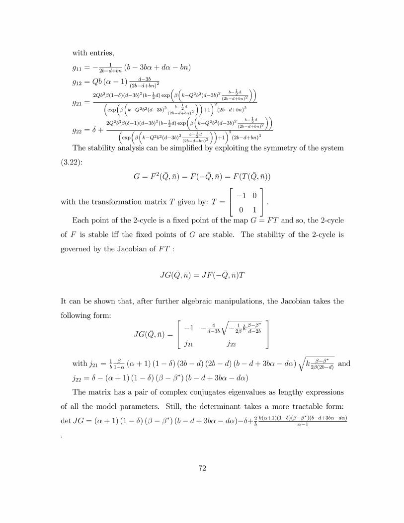
with entries,

g11 = � 12b�d+bn (b� 3b� + d�� bn)

g12 = Qb (�� 1) d�3b(2b�d+bn)2

g21 =2Qb2�(1��)(d�3b)2(b� 1

2d) exp

��

�k�Q2b2(d�3b)2 b� 1

2 d

(2b�d+bn)2

��exp

��

�k�Q2b2(d�3b)2 b� 1

2 d

(2b�d+bn)2

��+1

�2(2b�d+bn)2

g22 = � +2Q2b3�(��1)(d�3b)2(b� 1

2d) exp

��

�k�Q2b2(d�3b)2 b� 1

2 d

(2b�d+bn)2

��exp

��

�k�Q2b2(d�3b)2 b� 1

2 d

(2b�d+bn)2

��+1

�2(2b�d+bn)3

The stability analysis can be simpli�ed by exploiting the symmetry of the system

(3.22):

G = F 2( �Q; �n) = F (� �Q; �n) = F (T ( �Q; �n))

with the transformation matrix T given by: T =

24 �1 0

0 1

35 :Each point of the 2-cycle is a �xed point of the map G = FT and so, the 2-cycle

of F is stable i¤ the �xed points of G are stable. The stability of the 2-cycle is

governed by the Jacobian of FT :

JG( �Q; �n) = JF (� �Q; �n)T

It can be shown that, after further algebraic manipulations, the Jacobian takes the

following form:

JG( �Q; �n) =

24 �1 � 4d�3b

q� 12�k ��

�

d�2b

j21 j22

35with j21 = 1

b�1�� (�+ 1) (1� �) (3b� d) (2b� d) (b� d+ 3b�� d�)

qk ��2�(2b�d) and

j22 = � � (�+ 1) (1� �) (� � ��) (b� d+ 3b�� d�)

The matrix has a pair of complex conjugates eigenvalues as lengthy expressions

of all the model parameters. Still, the determinant takes a more tractable form:

det JG = (�+ 1) (1� �) (� � ��) (b� d+ 3b�� d�)��+2bk(�+1)(1��)(��)(b�d+3b��d�)

��1

:

72

The Neimark-Sacker bifurcation condition (det JG = 1) yields the intensity of

choice threshold �� at which a second bifurcation arises, namely:

�� = �� +1 + �

(1� �) (b� d+ �(3b� d)) (�+ 1) (1� 2b

k1��)

This completes the proof of Lemma 4.

Summing up, as the intensity of choice varies from low to high values the sys-

tem transits from a unique steady state, through a 2-cycle to two limit cycles at

� = �� when it undergoes a Neimark-Sacker bifurcation and each of the 2-cycle

branches becomes surrounded by a closed orbit as in Fig. 3.1d. Panels (a)-(b) illus-

trate the limiting behavior of quantities picked by the two players as they become

more responsive to payo¤ di¤erences, while Panel (c) displays the time evolution of

the proportion of the costly rational (or Nash) expectation-formation heuristic. The

intuition is similar to Brock and Hommes (1997): when the system is close to the

Cournot-Nash equilibrium the simple, costless adaptive rule performs well enough

and, due to the evolutionary switching mechanism, a larger number of players makes

use of this cheap heuristic. However with a vast majority of agents using adaptive rule

the CNE destabilizes and, as �uctuations of increasing amplitude arise, it pays o¤

to switch to the more involved, though costly, behavior (i.e. Nash) pays-o¤. Once

a large majority of agents switches to the rational rule �uctuations are stabilized

and agents switch back to the costfree heuristic, re-initializing the cycle. Fig. 3.2a-b

illustrates the primary (period-doubling) and secondary (Neimark-Sacker) bifurca-

tions along with the "breaking of the invariant circle" route to chaos as the intensity

of choice and degree of expectations adaptiveness are varied, respectively. Finally,

Panels (c)-(d) show a strange attractor in the quantity-fraction of Nash players and

quantity-quantity subspaces.

73

4 . 9

5 . 2

5 . 5

5 . 8

1 0 0 1 0 5 1 1 0 1 1 5 1 2 0

q 1q 2

(a) � = 2: Time series

4

5

6

7

1 0 0 1 0 5 1 1 0 1 1 5 1 2 0

q 1q 2

(b) � = 9: Time series

0

0 . 3

0 . 6

0 . 9

1 0 0 1 1 0 1 2 0 1 3 0 1 4 0

n

(c) � = 9: Evolution of fraction of RE (d) � = 5:2: Qasiperiodic behavior

Figure 3.1: Cournot duopoly game with an ecology of Adaptive and Rational players.Panels (a)-(b): quantities evolution for di¤erent values of the intensity of choice (�). Theevolution of Nash players fraction is shown in Panel (c). Panel (d) displays a limit cycle,consisting of two closed curves around the two points of the unstable 2-cycle, arising fromthe secondary Hopf bifurcation. Game parameters set to a = 17; b = 0:8; c = 10; d =1:1; k = 1; � = 0:05; � = 0:1:

74

(a) Bifurcation diagram: � � q1,� = 0:05 (b) Bifurcation diagram: �� q1; � = 15

(c) Strange attractor, q1 � n (d) Strange attractor, q1 � q2

Figure 3.2: Cournot duopoly game with an ecology of Adaptive and Rational players.Bifurcation diagrams of the equilibrium quantity chosen by the Adaptive players (q1) withrespect to the intensity of choice (�) (Panel (a)) and degree of expectation adaptiveness (�)in Panel (b). Game parameters set to a = 17; b = 0:8; c = 10; d = 1:1; � = 0:1. Panels (c),(d) display projection of a strange attractor on the quantity-fraction of rational players andquantity-quantity subspaces, respectively. A strange attractor is obtained for the followingparameterization: a = 17:54; b = 0:754; c = 10; d = 1:1; k = 1:5; � = 0:1; � = 7:8; � = 0:5:

75

3.4.2 Adaptive vs. Exponentially Weighted Fictitious Play

As was already pointed out, players form expectations about the strategy of the

average opponent given the existing heuristics ecology (frequencies of each learning

type). In this subsection, the subset available is restricted to Adaptive Expectations

and Weighted Fictitious Play as introduced in subsection 3.3. Thus, the rational

rule is replaced by a long-memory rule that relies only on past observed quantity

information with, possibly, di¤erent weighting schemes for each observation. Similar

to the previous sections, the more sophisticated heuristic comes at a cost k: Con-

sidering that a WFP process gives rise to a non-autonomous dynamical system we

will discuss analytically the limit as t!1 when the system becomes autonomous.

Let qeAE(t + 1) and qeWFP (t + 1) denote the expectations formed about an average

encountered opponent by an AE-player and a WFP-player, respectively. The evol-

ution of these two learning rules, in a Cournotian strategic environment is given by

the following system of di¤erence equations:

qeAE(t+ 1) � qe1(t+ 1) = �qe1(t) + (1� �)qavgopp (t)

qeWFP (t+ 1) � qe2(t+ 1) = qe1(t) + (1� )qavgopp (t)

with > �3: By letting n(t) denote the fraction of agents employing the more

computationally-involved heuristic II (WFP expectations in this case) this system

3In subsection 3.3 we have seen that � close to 0 renders adaptive expectations, while ap-proaching 1 yields the standard �ctitious play. These two parameters could also be interpreted asproxies for "memory": when they are close to the lower bound 0 the past is heavily discarded andonly recent observations matter for constructing expectations about opponent choice, while as theyare near the upper bound 1 past information becomes increasingly important for future choices.Thus naive expectations [� = 0] is a short-memory rule, as the entire past, but last period, isdiscarded, while �ctitious play [ = 1] is a long-memory rule, as each past observation is equallyimportant.

76

can be explicitly re-written as:

qe1(t+ 1) = �qe1(t) + (1� �)((1� n(t))q1(t) + n(t)q2(t)) (3.26)

qe2(t+ 1) = qe1(t) + (1� )((1� n(t))q1(t) + n(t)q2(t)) (3.27)

The actual strategic choices of anAE- andWFP -player are simply best-responses

to their expectations:

q1(t) = R(qe1(t)) =a� c� bqe1(t)

2b� d (3.28)

q2(t) = R(qe2(t)) =a� c� bqe2(t)

2b� d (3.29)

The fraction of the more sophisticated WFP players evolves according to an asyn-

chronous updating logistic mechanism (Hommes et al. (2005)):

n(t+ 1) = �n(t) + (1� �) exp(�(U2(t)� k))exp(�U1(t)) + exp(�(U2(t)� k))

; (3.30)

where U1; U2 represent the average pro�ts of an AE and WFP player at time t, and

� denotes the inverse of the noise/or "intensity of choice" parameter and k stands for

the extra-costs incurred by the agents employing the more sophisticated (i.e. with a

higher weight placed on past observations about opponent choices) WFP heuristic.

The performance measures U1; U2 are determined as in equations (3.16)-(3.17) from

subsection 3.4.1. Similarly, we derive a three-dimensional, discrete dynamical system

(qe1(t+1); qe2(t+1); n(t+1)) = �(q

e1(t); q

e2(t); n(t)) describing both the evolution of the

adaptive and �ctitious play type expectations and of the learning heuristics�ecology:

qe1(t+ 1) = �qe1(t) + (1� �)((1� n(t))R(qe1(t)) + n(t)R(qe2(t)))

qe2(t+ 1) = qe2(t) + (1� )((1� n(t))R(qe1(t)) + n(t)R(qe2(t))) (3.31)

n(t+ 1) = �n(t) +1� �

1 + e(�(U1(R(qe1(t));R(q

e2(t));n(t))�U2(R(qe1(t));R(qe2(t));n(t))+k))

77

Lemma 5 The (static) Cournot-Nash equilibrium quantities (q�1; q�2) determined in

(3.6) together with n� = 11+exp(�k)

is an (interior) �xed point of system (3.31).

Proof. At the Cournot-Nash Equilibrium(CNE) q�1 = q�2 =a�c3b�d we have, by

de�nition, R(qe1(t)) = qe1(t) and R(q

e2(t)) = q

e2(t):Substituting into the �rst two equa-

tions of (3.31) gives the required �xed point equality. Then, n� = 11+exp(�k)

is the

solution of n(t+ 1) = n(t) when this equation is evaluated at the CNE.

3.4.3 Local stability analysis

It can be shown that the Jacobian matrix of (3.31) evaluated at the equilibrium

(q�1; q�2; n

�) takes the following form:

J�=SS =

26664�+ (1� �)(1� n�)r (1� �)n�r 0

(1� )(1� n�)r + (1� )n�r 0

0 0 �

37775 (3.32)

where r = @R(qei )

qei= � b

2b�d ; r < �1:

We know that under homogenous, naive (or adaptive with small �) expectations

the CNE is unstable with a two- cycle emerging at the boundary. On the other hand,

�ctitious play alone (or weighted �ctitious play with large weights put in remote past

observations) stabilizes the CNE. Once the interplay between the cheap adaptive and

costly WFP heuristics is introduced we can prove the following result:

Proposition 6 A system with evolutionary switching between adaptive and weighted

�ctitious play expectations (i.e. 0 < � � < 1) is destabilized when the sensit-

ivity to payo¤ di¤erence between alternative heuristics reaches a threshold �PD =

1kln (r�1)�(1+�)(r+1)

( +1)(r+1)+�(1�r) and a stable two-cycle bifurcates from the interior CN steady

state (q�1 = q�2 =

a�c3b�d ; n

� = 11+exp(�k)

):

Proof. For an ecology of Adaptive and Weighted Fictitious Play rules - � 2

78

(0; 1); 2 (0; 1); � � = the eigenvalues of the Jacobian matrix (3.32) are : �1;2 =12r + 1

2�+ 1

2 � 1

2r� + 1

2r�n� � 1

2r n� � 1

2

pS; �3 = �

with S = r2�2(n�)2 � 2r2�2n� + r2�2 � 2r2� (n�)2 + 2r2� n� + 2r2�n�

�2r2�+ r2 2(n�)2 � 2r2 n� + r2 + 2r�2n� � 2r�2 + 2r� � 4r�n�

+2r�� 2r 2n� + 4r n� � 2r + �2 � 2� + 2

Next the period-doubling condition �2 = �1 yields:

n�(�) =(1 + )[(1 + r) + �(1� r)]

2r( � �)

�PD =1

kln (r � 1)� (1 + �) (r + 1)( + 1) (r + 1) + �(1� r) (3.33)

We can also derive the intensity of choice threshold at which instability arises for

an ecology of Naive vs. Weighted Fictitious Play - � = 0; 2 (0; 1) - as a special

case of (3.33):

�PD = �� =1

klnr( � 1)� (1 + )( + 1) (r + 1)

For an ecology of Fictitious vs. Adaptive Players - = 1; � 2 (0; 1) - system

(3.31) is non-autonomous and we will investigate this case in a subsequent section,

numerically.

We notice that if there are no costs associated with the sophisticated predictor

WFP (i.e. k = 0) the system is stable for any value of the intensity of choice. This

is so because what trigger switching into the destabilizing adaptive rule are the costs

incurred when usingWFP : thus, for k = 0 there is no incentive to switch away from

WFP even in tranquil or stable periods.

The 2-cycle, in deviations from the Cournot -Nash steady state - ((x; y; n); (X; Y; n))

79

with X = �x; Y = �y - solves the following system of equations:

X = �x+ (1� �)((1� n)a�c�bx2b�d + na�c�by

2b�d )�(a�c)(1��)

2b�d

Y = y + (1� )((1� n)a�c�bx2b�d + na�c�by

2b�d )�(a�c)(1� )

2b�d

x = �X + (1� �)((1� n)a�c�bX2b�d + na�c�bY

2b�d )�(a�c)(1��)

2b�d

y = Y + (1� )((1� n)a�c�bX2b�d + na�c�bY

2b�d )�(a�c)(1� )

2b�d

n = �n+ 1��exp( 1

2b2

(d�2b)2) exp(�((x�y)(2a�2c�4bx�2by+dx+dy+2bnx�2bny)+k))

(3.34)

Given that the two-cycle above satis�es X = �x; Y = �y , we obtain, after some

manipulations, that the ratio of the two expectation rules deviations from equilibrium

prediction is given by:x

y=(1� �)=(1 + �)(1� )=(1 + )

For � � (an adaptive vs. �ctitious play ecology) we get x > y. Thus, the

�uctuations of the adaptive, short-memory rule exceed in amplitude the oscillations

incurred by the long memory heuristic (see Fig. 3.3ab).

If we analyze the time evolution of the costly WFP fraction we observe a similar

pattern as for the naive vs. Nash ecology discussed in the previous subsection. In

tranquil times, when the dynamics is close to the Cournot-Nash equilibrium, the

cheap adaptive rule outperforms the more involved and costly WFP rule. Thus,

through the selection mechanism, almost the entire population becomes adaptive.

However, a Cournot duopoly with adaptive(near naive) expectations is unstable and,

as �uctuations emerge, conditions are created for the costly, more sophisticatedWFP

rule, to take over the population and re-stabilize the system.

We can also show, numerically, that the 2-cycle loses stability via a secondary

Neimark-Sacker bifurcation with a quasi-periodic attractor consisting of two closed

curves, arising around the unstable branches of the 2-cycle (Fig. 3.3d). Furthermore,

the invariant curves break into a strange attractor if the intensity of choice � is

increased even further. Bifurcations diagrams with respect to di¤erent behavioral

80

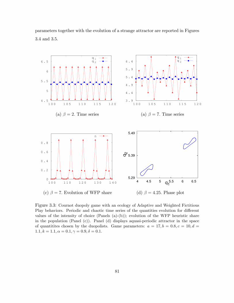
parameters together with the evolution of a strange attractor are reported in Figures

3.4 and 3.5.

4 . 5

5

5 . 5

6

6 . 5

1 0 0 1 0 5 1 1 0 1 1 5 1 2 0

q 1q 2


3 . 9

4 . 4

4 . 9

5 . 4

5 . 9

6 . 4

1 0 0 1 0 5 1 1 0 1 1 5 1 2 0

q 1q 2


0

0 . 2

0 . 4

0 . 6

0 . 8

1 0 0 1 1 0 1 2 0 1 3 0 1 4 0

n

(c) � = 7: Evolution of WFP share (d) � = 4:25: Phase plot

Figure 3.3: Cournot duopoly game with an ecology of Adaptive and Weighted FictitiousPlay behaviors. Periodic and chaotic time series of the quantities evolution for di¤erentvalues of the intensity of choice (Panels (a)-(b)); evolution of the WFP heuristic sharein the population (Panel (c)). Panel (d) displays aquasi-periodic attractor in the spaceof quantitites chosen by the duopolists. Game parameters: a = 17; b = 0:8; c = 10; d =1:1; k = 1:1; � = 0:1; = 0:9; � = 0:1:

81

(a) Bifurcation diagram, �� q1; = 0:9 (b) Bifurcation diagram, � q1; � = 0:1

(c) Bifurcation diagram,

� � q1; � = 0:1[AE], = 0:9[WFP ]

(d) Bifurcation diagram,

e� q1; � = 0:1[AE], = 0:9[WFP ]

Figure 3.4: Cournot duopoly game with an ecology of Adaptive and Weighted FictitiousPlay behaviors. Panels (a)-(d): bifurcation diagrams of the equilibrium quantity picked bythe Adaptive type (q1) with respect to degree of expctation adaptiveness (�), weightingparameter in the WFP rule ( ), intensity of choice (�) and costs associated with WFP(e), respectively. Game parameters: a = 15; b = 0:7; c = 10; d = 1:1; k = 1:1; � = 0:1; =0:9; � = 12; � = 0:1:

82

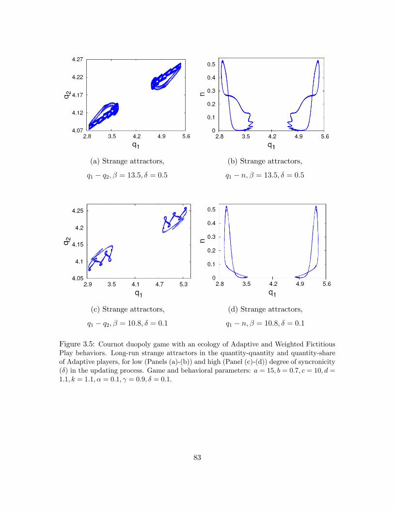
(a) Strange attractors,

q1 � q2; � = 13:5; � = 0:5

(b) Strange attractors,

q1 � n; � = 13:5; � = 0:5

(c) Strange attractors,

q1 � q2; � = 10:8; � = 0:1

(d) Strange attractors,

q1 � n; � = 10:8; � = 0:1

Figure 3.5: Cournot duopoly game with an ecology of Adaptive and Weighted FictitiousPlay behaviors. Long-run strange attractors in the quantity-quantity and quantity-shareof Adaptive players, for low (Panels (a)-(b)) and high (Panel (c)-(d)) degree of syncronicity(�) in the updating process. Game and behavioral parameters: a = 15; b = 0:7; c = 10; d =1:1; k = 1:1; � = 0:1; = 0:9; � = 0:1:

83

3.4.4 Naive vs. Fictitious Play

In this subsection we report numerical simulations of the long-run behavior of the

evolutionary competition between costless naive expectations and costly �ctitious

play for a linear inverse demand-quadratic costs quantity-setting duopoly. This eco-

logy combines, in a sense, two limiting results from the previous subsections: Cournot

or naive expectations - as � ! 0 - along with standard �ctitious play expectations

- as ! 1: It is known that �ctitious play converges in a homogenous popula-

tion of �ctitious players to Cournot-Nash equilibrium while naive expectations alone

generate continuous oscillations. Hence, a natural question to ask is whether the

presence of �ctitious players could stabilize a population of naive players. Fig. (3.6)

presents numerical simulations of the competition between the two heuristics and

show persistent �uctuations of the naive players quantity around the Cournot-Nash

equilibrium. The share of �ctitious players (Fig. 3.6c) lingers close to extinction and

spikes occasionally taking over almost the entire population. Similar to the previous

two subsections, what is driving this results are the costs associated with the �cti-

tious play rule: when the entire population follows the FP rule, the CNE is stabilized

and so there is an incentive to switch to the cheaper rule, i.e. adaptive heuristic. As

more and more players become adaptive the CNE loses stability, �uctuations emerge

and ,thus, they create an advantageous environment for long-memory players to step

in. Depending on the intensity of selection (as captured by parameter �) the �uc-

tuations could be periodic (Panel(a)) of even chaotic: see Panel (d) in Fig. 3.6 for

numerical plot of the largest Lyapunov exponent. Fig. 3.7a-d depicts the evolution

of such an attractor as the sensitivity to material payo¤s � varies. In order to escape

the long transient of the �ctitious play dynamics, the phase portraits are plotted

after skipping 100; 000 points of the series. While the �ctitious player quantities

stay within a small neighborhood the Cournot-Nash equilibrium, the strategies of

the Cornout(naive) player display chaotic �uctuations of large amplitudes.

84

3

4

5

6

7

1 0 0 1 0 5 1 1 0 1 1 5 1 2 0

q 1q 2


2 . 6

3 . 6

4 . 6

5 . 6

6 . 6

1 0 0 1 0 5 1 1 0 1 1 5 1 2 0

q 1q 2


0

0 . 3

0 . 6

0 . 9

1 0 0 1 1 0 1 2 0 1 3 0 1 4 0 1 5 0

n

(c) � = 6: Evolution of FP share

0 . 1

0

0 . 1

0 . 2

0 . 3

0 1 2 3 4 5 6

Lyapunov exp.

β

(d). Largest Lyapunov exponent

Figure 3.6: Cournot duopoly game with Naive and Fictitious Play Heuristics. Pattern ofplay evolution for naive and �ctitious players, for di¤erent values of the intensity of choicein Panels (a) and (b), respectively. Panel (c) shows the time evolution of Fictitious Playfraction while Panel (d) provides numerical evidence for chaotic dynamics for large values of�. Game and behavioral parameters: a = 17; b = 0:8; c = 10; d = 1:1; k = 1; � = 0; � = 0:1:

85

(a) � = 1:65 (b) � = 2:22

(c) � = 2:65 (d) � = 5:38

Figure 3.7: Cournot duopoly game with Naive and Fictitious Play Heuristics. Panels (a)-(d): the evolution of the phase portrait into a strange attractor as the intensity of choiceincreases. Notice that the quantity picked by the �ctitious player wanders around theCournot-Nash equilibrium quantity while the output choice of the naive players exhibitsmore wide chaotic �uctuations around the same CNE. Game and behavioral parameters:a = 17; b = 0:8; c = 10; d = 1:1; e = 1; � = 0; � = 0:1:

86

3.5 Concluding Remarks

We studied evolutionary Cournot games with heterogenous learning rules about

opponent strategic quantity or price choice. The evolutionary selection of such �learn-

ing�heuristics is driven by a logistic-type evolutionary dynamics. While our focus is

on the interplay between adaptive and ��ctitious play�expectations, other rules eco-

logies(e.g. weighted �ctitious play vs. rational or Nash expectations) are explored,

as well. Analytical and simulation results about the behaviour of the corresponding

evolutionary Cournot games, when various parameters of interest change, are presen-

ted. In a Cournotian setting, the main �nding is that a population of (weighted)

�ctitious players (i.e best-responders to the empirical distribution of past history of

opponent choices) could be destabilized away from the Cournot-Nash equilibrium

play by the presence of the adaptive expectation formation rule (i.e. players who

place large weight on the last period choice and heavily discard more remote past

observations). The interaction between a costly weighted �ctitious play and the

cheap adaptive expectations yields complicated quantity dynamics. The key mech-

anism driving dynamics is the endogenous switching between learning rules based on

realized �tness: The �ctitious play drive the system near the Cournot-Nash equilib-

rium where the simple, adaptive rule performs relatively well and, due, to its cost

advantage, can invade and take over the more sophisticated predictor. However, the

adaptive rule alone destabilizes the interior equilibrium and, when far from the CNE

it pays o¤ to bear the costs of the more involved rule reinitializing the evolutionary

cycle.

87

Chapter 4

On the Stability of the Cournot

Solution: An Evolutionary

Approach

4.1 Introduction

Within a linear cost-linear demand set-up, Theocharis (1960) shows that once

the duopoly assumption is relaxed and the number of players increases, the Cournot

Nash equilibrium loses stability and bounded oscillations arise already for triopoly

quantity-setting games. For more than 3 players oscillations grow quickly unbounded

but they are stabilized by the non-negativity price and demand constraint. Hahn

(1962) puts forth an alternative proof of this results and derives stability conditions

for asymmetric cost functions and nonlinear cost and demand functions. Fisher

(1961) and McManus (1964) recover stability of the equilibrium when �rms use,

instead of the discrete-time best response dynamic of Theocharis (1960), a continuous

adjustment process to some optimally derived output target. However, �rms do these

adjustments incompletely (i.e. with di¤erent speeds of adjustment) at each time

instance. In this class of adjustment processes, increasing the marginal costs acts as

89

a stabilizer of the Cournot-Nash equilibrium, irrespective of the number of players.

In Okuguchi (1970) both the actual output and expectations of rivals�output follow

a continuous adjustment process to some target and restrictions on the speeds of

adjustment (of both actual and the rival�s expected output) are derived in relation

to the rate of marginal costs increase such that stability is regained for an arbitrary

number of players. Adaptive expectations generalize Cournot (naive) expectations.

Thus, in a multi-player oligopoly game, where players follow a discrete-time best-

response to adaptively formed expectations about rivals output, Szidarovszky et al.

(1994) �nd suitable restrictions on the coe¢ cients of adaptive expectations such that

the unique Cournot-Nash equilibrium is stabilized.

In this short Chapter we take a di¤erent route and relax the assumption of homo-

genous expectations, while preserving the linear structure and best-reply adjustment

dynamics of Theocharis (1960). The questions we address is whether Theocharis

(1960) classical instability result still persist under the evolutionary selection of het-

erogenous expectations rule. We show that, in an evolutionary environment, the

instability is robust to a heterogenous ecology of heuristics. In particular, we focus

on the interplay between a simple adaptive rule and a more involved, but costly,

rational rule with agents choosing the best-performing rule according to a logistic

updating mechanism. The threshold number of players that triggers instability may

vary with the costs of the rational expectations rule or with the adaptive expectations

coe¢ cient.

In Section 4.2 the model is introduced, results and simulations are reported in

Section 4.3 while Section 4.4 contains some concluding remarks.

90

4.2 The model

We start with the Theocharis (1960) simple linear inverse demand-linear costs

homogenous, n-player oligopoly game. Linear inverse demand is given by

P = a� bnXi=1

qi; (4.1)

and linear costs by

Ci(qi) = cqi: (4.2)

Each period n players are drawn from a large populations to play a n-player

quantity-setting game. Furthermore, assume that the population of oligopolists con-

sists of two behavioural types: adaptive players (share 1 � p in the population)

playing quantity q1 and rational (share p) picking quantity q2: From the perspective

of an individual player the aggregate output of the remaining n�1 opponents, given

behavioral types, could be computed for di¤erent market structures as follows:

In the triopoly case the two randomly drawn opponents may be, with probability

p2 of rational type (producing q2 each), with probability (1�p)2 of adaptive type (and

thus choosing q1 each) and, with probability 2p(1�p) of di¤erent types (thus picking

q1 and q2; respectively). Thus, the output of an average opponent in a triopoly game

is given by:

p22q2 + 2p(1� p)(q2 + q1) + (1� p)22q1 (4.3)

Similarly, for the quadropoly Cournot game we get

p33q2 + 3p2(1� p)(2q2 + q1) + 3p(1� p)2(q2 + 2q1) + (1� p)33q1 (4.4)

91

and for quintopoly:

p44q2+4p3(1�p)(3q2+q1)+6p2(1�p)2(2q2+2q1)+4p(1�p)3(3q2+3q1)+(1�p)44q1

(4.5)

More generally, in the n-player quantity-setting game the output of an average

opponent is given by:

n�1Xk=o

��n

k

�pk(1� p)n�1�k((n� 1� k)q1 + kq2)

�

= q2

n�1Xk=o

��n

k

�pk(1� p)n�1�kk

�+ q1

n�1Xk=o

��n

k

�pk(1� p)n�1�k(n� k � 1)

�= q2(n� 1)p+ q1(n� 1)(1� p) (4.6)

The aggregate expected output of the n�1 opponents is equivalent to the output

of n�1 averaged-across-types opponents. Thus, each player has to form expectations

about the output chosen by the average type in the population.

The adaptive type (AE) forms adaptive expectations about average the opponent:

qe1(t+ 1) = �qe1(t) + (1� �)[q1(t)(1� p) + q2(t)p)]: (4.7)

The rational type (RE) has perfect foresight:

qe2(t+ 1) = q1(t+ 1)(1� p) + q2(t+ 1)p): (4.8)

Both AE and RE types best-respond to expectations:

q1(t+ 1) = R1(qe1(t+ 1)) =

a�c�b(n�1)qe1(t+1)2b

q2(t+ 1) = R2(qe2(t+ 1)) =

a�c�b(n�1)qe2(t+1)2b

(4.9)

92

q2(t) = R2(qe2(t)) =

a� c� b(n� 1)qe2(t)2b

=a� c� b(n� 1)[q1(t)(1� p) + q2(t)p)]

2b(4.10)

q2(t) =a� c� bq1(t) (n� 1) (1� p)

2b�12p (n� 1) + 1

� (4.11)

After substituting (4.9) and (4.11) into (4.7) we obtain the adaptive expectations

dynamics as:

qe1(t+1) = �qe1+(1��)[R1(qe1(t))(1�p)+

a� c+ bR1(qe1(t)) (n� 1) (1� p)2b�12p (n� 1) + 1

� p)] (4.12)

Next, we compute the expected pro�ts as:

�1(t) = q1(t)[a� b[q1(t) + (n� 1)[q1(t)(1� p) + q2(t)p)]]� c]

�2(t) = q2(t)[a� b[q2(t) + (n� 1)[q1(t)(1� p) + q2(t)p)]]� c]

The share p of rational players updates according to asynchronous updating (only

a fraction 1 � � revise strategies according to the logistic probability) based on the

realized performance measure:

p(t+ 1) = �p(t) +1� �

1 + e(�(�1(R(qe1(t));R(q

e2(t));p(t))��2(R(qe1(t));R(qe2(t));p(t))+k))

(4.13)

where k stands for the costs associated with the rational expectations predictor

(see the discussion regarding asyncronous logistic updating in Chapter 3). Equations

(4.12) and (4.13) de�ne a two dimensional dynamical system (qe1(t+ 1); p(t+ 1)) =

�(qe1(t); p(t)) which has an interior steady state at:

(qe�1 =a� cb(1 + n)

; p� =1

1 + exp(�k))

93

Expressed in terms of actual quantity choices the steady state is:

q�1 = q�2 =

a� cb(1 + n)

; p� =1

1 + exp(�k)(4.14)

Before proceeding to the stability analysis of this equilibrium, we present in Fig.

4.1 simulations of the system behavior for varying number of players. As the game

changes from triopoly to a large number of players the interior Cournot-Nash equi-

librium (4.14) loses stability and bounded, regular or irregular oscillations arise. We

identify a period-doubling route to strange attractors as the number of players in-

creases.1. A snapshot of such a strange attractor is captured in Fig. 4.1e along with

numerical evidence (strictly positive largest Lyapunov exponent) for chaos in Panel

(f).

1This bifurcation diagram should be interpreted under the caveat that n is not a continousparameter (the number of players in the Cournot game only takes positive integers value) . Still,the bifurcation diagram can provide some information about qualitative changes in the behavior ofthe system, given the number of players.

94

0

0 . 6

1 . 2

1 . 8

2 . 4

0 5 1 0 1 5 2 0 2 5 3 0

q 1

(a) Time series, triopoly [n = 3]

0 . 5

1

1 . 5

2

0 5 1 0 1 5 2 0 2 5 3 0

q 1

(b) Time series, quadropoly [n = 4]

0

0 . 5

1

1 . 5

0 5 1 0 1 5 2 0 2 5 3 0

q 1

(c) Time series, octopoly [n = 8] (d) Bifurcation diagram q1 � n

(e) Phase plot, octopoly [n = 8]

0 . 8

0 . 5

0 . 2

0 . 1

0 . 4

2 4 6 8 1 0

Lyapunov exp.

n

(f) Largest Lyapunov exponent

Figure 4.1: Linear n-player Cournot game with an ecology of Adaptive and Rationalplayers. Panels (a)-(c) display converging, oscillating and chaotic time series of the quantityq1 chosen by the Adaptive type for 3; 4 and 8-player game, respectively. Instability sets inalready for the quadropoly game (Panel (b)). Panel (d) depicts a period-doubling routeto chaotic dynamics in equilibrum quantity q1 as we increase the number of players n. Atypical phase portrait for an 8-player game is shown in Panel (e) while Panel (f) providesnumerical evidence for chaos (i.e. positive largest Lyapunov exponent) as number of playersincreases. Game and behavioral parameters: a = 17; b = 1; c = 10; k = 1; � = 0:1; � =2:8; � = 0:1: 95

4.3 Results

We start with the following:

Proposition 7 The Cournot-Nash equilibrium (qe�1 = a�cb(1+n)

; p� = 11+exp(�k)

) loses

(local) stability as the number of player n reaches a critical threshold nPD = 2p��32p�+��1

and a 2-cycle in the equilibrium quantities is born via a period-doubling bifurcation.

Proof. We can rewrite system in deviations from the Cournot-Nash steady-state

Q(t) = a�cb(1+n)

� qe�1 (t) :

Q(t+ 1) = Q(t)(1 + �� (n+ p(t)) + n(�+ p(t)))

p(t)(n� 1) + 2 (4.15)

p(t+ 1) =1� �

1 + exp(�(�Q(t)(n2�1)(Q(t)bn2+2cpn+4c�Q(t)b�2cp)

4n2p2�8np2+16np+4p2�16p+16 + k))(4.16)

with the interior steady state: (Q� = 0; p� = 11+exp(�k)

): The Jacobi matrix at this

steady state is: 24 1p�(n�1)+2 (�� n� p

� + n (�+ p�) + 1) 0(4c�2cn+2cnp�)�p�(��1)(p��1)((p�)2�1)4n2(p�)2�8n2p�+4n2+16np��16n+16 �

35 ;with corresponding eigenvalues �1 = 1

np��p�+2 (�� n� p� + n� + np� + 1) and �2 =

�: The period-doubling bifurcation (�1 = �1) condition reads:

1

np� � p� + 2 (�� n� p� + n�+ np� + 1) = �1;

which yields,

nPD =2p� � �� 32p� + �� 1 : (4.17)

We notice �rst that the Cournot-Nash equilibrium is stable if the rational pre-

dictor is costless. The threshold (4.17) can be re-arranged as �PD = 1kln�(�+1)(1+n)n��(1+n)+3

�96

and observe that there is no �nite value of the intensity of choice satisfying this equal-

ity for costless RE (i.e. k = 0):

4.3.1 Best-response dynamics limit, � !1

We can now derive Theocharis (1960) unstable triopoly result (i.e. bounded oscilla-

tions for n = 3 and exploding oscillations for n = 4) in the limit of naive expectations

[�! 0] and best-response dynamics [� !1]. First we compute lim�!1 p� = 0 and

then evaluate the period-doubling threshold (4.17) at �! 0 yielding

lim�!1;�!0

nPD(p�(k)) = 3: (4.18)

The intuition behind the original "two is stable, three is unstable" result had to

do with the slope of a reaction curves (4.9)��@R@q �� = ��n�1

2

�� : For a duopoly gamethis slope is, in absolute values, always smaller than 1; but it hits the instability

threshold exactly at n = 3 and is larger than 1 starting for a quadropoly game. This

is exactly what our threshold nPD boils down to when we let players choose a best

reply [� !1] to Cournot (i.e. naively-determined) expectations [�! 0]:

Some further comparative statics can be informative about the role expectations

play in (de) stabilizing a Cournot-Nash equilibrium. Ceteris paribus, the number of

players�instability threshold n� increases in the degree of expectation adaptiveness

[�]:

@nPD=@� = 41� p�

(�+ 2p� � 1)2> 0:

Intuitively, a larger � implies that the unstable adaptive rule place a higher

weight on remote observations in the past and thus it acts as an e¤ective stabilizing

force. This, in turn, requires an even larger slope of the reaction curve (i.e. larger

threshold n�) to de-stabilize the interior CN equilibrium. Similarly, we can show that

97

n� decreases in the costs associated with the perfect foresight rule:

@nPD(p�(k))=@k < 0;

as @nPD(p�)=@p� = 4 �+1(2p+��1)2 > 0 and @p

�=@k < 0:

For a given number of players, at the steady state, higher costs of rational expect-

ations k; increase the payo¤di¤erential between the rational and the naive heuristics.

Hence, more agents switch to the simple, yet destabilizing adaptive strategy. Thus,

the system becomes more unstable and it takes a less steeper reaction curve (i.e.

fewer players) to hit the period-doubling threshold (4.17).

4.3.2 Costly Rational Expectations, k > 0 and �nite �

In the sequel we derive the threshold number of �rms for which instability arises

when there are positive costs associated with the perfect foresight and the other

behavioural rule approaches either the Cournot (� = 0) or adaptive expectations

(e.g. � = 0:2). Recall from (4.17) that nPD = 2p��32p�+��1 and p

� = 11+exp(�k)

: For small

costs of the rational predictor (k = 1) the period-doubling threshold is hit at:

nPDk=1 =�+ 3e� + �e� + 1

e� � �� e� � 1 (4.19)

Table 4.1 reports unstable market structures in evolutionary Cournot games (i.e.

number of players�period-doubling, rounded thresholds (4.19)) for di¤erent adaptive

expectations rule � and intensity of choice �:

98

�=� 1 - "low" 5 - "high"

0 ("Cournot" expectation) 5 (quintopoly) 3 (triopoly)

0:2 ("adaptive" expectations) 10 (decapoly) 4 (quadropoly)

Table 4.1: Linear n-player Cournot game with costly Rational expectations. Unstablemarket structures for di¤erent expectations and behavioral parameterization. Game andbehavioral parameters: a = 17; b = 1; c = 10; k = 1; � = 0:1:

These analytically derived thresholds are con�rmed by the numerically-computed

bifurcations curves illustrated Fig. 4.2a-d. Higher values of the intensity of choice

may destabilize a given market structure: larger � e¤ectively implies turning on

the evolutionary selection mechanism built into the model and population switching

into/away from the adaptive, unstable heuristic. The two bottom panels in Fig. 4.2

display, for a quintopoly game, a strange attractors in the quantities chosen by the

two types in the population (Panel (e)) and fractions of rational players-deviations

from steady state quantity (Panel (f)).

99

(a) � = 0; � = 1: nPD =Quintopoly (b) � = 0; � = 5: nPD =Triopoly

(c) � = 0:2; � = 1: nPD =Decapoly (d) � = 0:2; � = 5: nPD =Quadropoly

(e) n = 5; � = 0:2; � = 10:65 (f) n = 5; � = 0:2; � = 10:65

Figure 4.2: Linear n-player Cournot game with costly Rational expectations. Bifurcationdiagrams of the deviations Q from equilibrium quantity q1 with respect to number of �rmsn for Naive [� = 0] (Panel (a), (b)) and Adaptive [� = 0:2] (Panel (c), (d)) expectations.Panels (a)-(d): The �rst period-doubling bifurcation threshold decreases in the intensityof choice parameter �. Panels (e)-(f) display projection of a strange attractor onto thequantity-quantity and deviations from CNE quantity-fractions of RE players, respectively.Game and behavioral parameters: a = 17; b = 1; c = 10; k = 1; � = 0:1:

100

4.4 Conclusions

We constructed an evolutionary version of Theocharis (1960) seminal work on the

stability of the Cournotian equilibrium in multi-player quantity-setting games. The

assumption of homogenous naive expectations is relaxed and players are allowed to

choose between a costless, adaptive rule and a costly, rational rule. The results are

consistent with the original homogenous-expectations analysis of Theocharis, but the

instability thresholds vary with the costs of the sophisticated rule and the degree of

adaptiveness in the expectation formation process. One implication of the model

is that by �ne-tuning these two parameters a particular Cournot market structure

can be (de)stabilized. For instance, the classical unstable Cournot triopoly may

be stabilized via making the rational expectations predictor freely available. On the

other hand, when rational expectations are costly a period-doubling bifurcation route

to chaos arises when the number of players increases.

101

Chapter 5

Evolution in Iterated Prisoner�s

Dilemma Games under Smoothed

Best-Reply Dynamics

5.1 Introduction

Studying evolutionary dynamics on iterated prisoner�s dilemma (IPD) demands a

selection out of the vast set of the repeated game strategies. This choice turns out

to be important for the outcome of the iterated game and the level of cooperation

�evolved�. For instance, although the Tit-For-Tat strategy was an undisputed winner

of two round-robin tournaments, Axelrod (1997) stresses the crucial role of the sur-

rounding ecology of submitted iterated rules for the success of this direct reciprocity

norm. However, which strategies to choose out of the large set of repeated PD is a

question lacking a de�nite answer in the literature. Kraines and Kraines (2000) de�ne

adaptive dynamics1 on the space of memory one repeated PD strategies and show

that this process selects, as long-run outcome, only three classes of repeated rules:

1Adaptive dynamics are regularly used in evolutionary biology to model evolution through nat-ural selection on the �tness landscape.

103

cooperative, alternating and defective. They also claim that, out of the cooperative

subset, the Pavlov strategy is the only one that cannot be invaded by a strategy from

the same �cooperative�class (including TFT). Sigmund and Brandt (2006) investig-

ate one such ecology consisting of three strategies: unconditional cooperators (AllC),

unconditional defectors (AllD) and reactive players (TFT) and show that Replicator

Dynamics exhibits, among others, a rock-scissors-paper pattern of cyclic behavior.

However, as we have seen in Chapter 2, such replicator cycles are not robust under

Replicator Dynamics, as small payo¤ perturbations drive all but one strategy near

to extinction2.

In this chapter, we contribute to the stream of work on evolution of rules in re-

peated games by analyzing the repeated Prisoner�s Dilemma with a small number of

simple, memory-one strategies. In particular, we extend Sigmund and Brandt (2006)

ecology with two additional repeated strategies that seem to have received less atten-

tion in the evolutionary IPD game literature: the error-proof, "generous" tit-for-tat

which, with a certain probability, re-establishes cooperation after a (possibly by mis-

take) defection of the opponent and the penitent, "stimulus-response" (thus dubbed

Pavlov strategy Kraines and Kraines (1995), Sigmund and Nowak (1993b), Sigmund

and Nowak (1993a)) that resets cooperation after the opponent punished for defec-

tion. Second, we contrast Replicator Dynamics behavior with a perturbed version of

the Best-Reply dynamics, the Logit Dynamics, allowing for an imperfect switching

towards a myopic best reply to the existing strategies distribution. Our emphasis

is on the possibility of complicated dynamics such as multiplicity of steady states,

limit cycles or chaos in the resulting dynamical system. We start with a systematic

investigation of all ten 2 � 2 repeated game rules interactions and then build-up

towards more complex ecologies of 3, 4, and 5 strategies, combining theoretical con-

siderations about the best-reply structure of the resulting normal form games with

2mathematically, a so-called heteroclinic cycle is born, with Replicator Dynamics trajectorieslingering longer and longer near the boundary of the simplex.

104

numerical analysis and simulations. A bifurcation analysis with respect to various

model parameters is performed in order to reveal qualitative changes in the set of

long-run (non)cooperative behaviors. Preliminary results, in particular for the 4� 4

and 5 � 5 IPD ecologies, show that Logit Dynamics displays stable co-existence of

repeated strategies but subjected to perpetual oscillations or even chaotic patterns

in the distribution of IPD strategies.

The chapter is structured as follows: Section 5.2 introduces the selection of iter-

ated PD strategies and the resulting evolutionary IPD game. The 2; 3 and 4�types

ecologies are discussed in Sections 5.3, 5.4 and 5.5, respectively, while Section 5.6 in-

vestigates, mainly via computer simulations, the full 5� 5 ecology. The �nal section

is reserved for concluding remarks and future research directions.

5.2 An Evolutionary Iterated PD game

We consider a standard 2x2 Prisoner�s Dilemma stage game where players can either

cooperate (C) or defect (D). The payo¤ matrix of the stage game is given by:

26664C=D C D

C b� c; b� c �c; b

D b;�c 0; 0

37775 ; b > c > 0 (5.1)

where b stands for the bene�ts of cooperation and c for the costs associated with

cooperative behavior. At each time t the state of the play between two opponents

is given by an element belonging to set : = fCC;CD;DC;DDg. For the iterated

PD game we restrict the choice of iterated Prisoner�s Dilemma meta-rules to a set

of stochastic memory-one strategies (see, for instance, Kraines and Kraines (2000)).

Our motivation for such a simple subset of IPD strategies resides, on the one hand, on

our attempt to model a particular form of boundedly rational players (namely limited

memory agents or forgetting e¤ects) and, on the other hand, to obtain analytical

105

tractability of the resulting Markov chain. The IPD game starts with a �rst random

move C orD and then proceeds with playing C with probability (r; s; t; p) conditional

on the realized state at time t�1 being CC;CD;DC;DD, respectively. Deterministic

strategies are particular limits in this stochastic strategy space. In particular we focus

on 5 well-known strategies:

� unconditional cooperators AllC : (1; 1; 1; 1);

� unconditional defectors AllD : (0; 0; 0; 0);

� conditional cooperators "Tit-for-Tatters" TFT : (1; 0; 1; 0);

� generous cooperators "Generous-Tit-for-Tat" GTFT : (1;m; 1; n)3;

� penitent or Pavlov players "WinStayLoseShift" WSLS : (1; 0; 0; 1).

Stochastic strategies are "�perturbations of the deterministic ones, where " has

the natural interpretation of a probability of mistakes or errors in implementa-

tion/execution of the deterministic strategies. Following Kraines&Kraines (2000)

the iterated Prisoner�s Dilemma game between two stochastic players S1 = (r; s; t; p)

and S2 = (x; y; z; w) leads to a Markov chain on states CC;CD;DC;DD with trans-

ition probabilities given by:

T =

26666666664

state CC CD DC DD

CC rx sz ty pw

CD r(1� x) s(1� z) t(1� y) p(1� w)

DC (1� r)x (1� s)z (1� t)y (1� p)w

DD (1� r)(1� x) (1� z)(1� s) (1� t)(1� y) (1� p)(1� w)

37777777775(5.2)

Each column of the matrix T in (5.2) contains transition probabilities to states

CC, CD, DC, DD, respectively and naturally, its entries add up to one. For instance,

3m stands for the probability of cooperating after the opponent defected and n is the probabilityof playing cooperate after mutual defection.

106

in the �rst column, entry t11 gives the probability of next period state staying in CC :

row player S1 cooperates with probability r after the realized state was CC while

column player S2 cooperates with probability x after the same realization, and thus:

t11 = prob(CC j CC) = rx:

Similarly,

t21 = prob(CD j CC) = prob(S1 cooperates after CC)� prob(S2 defects after CC)

= r � (1� prob(S2 cooperates after CC)) = r(1� x):

One can show that, for strictly positive perturbation parameters, this Markov pro-

cess is ergodic, i.e. there is positive probability of escaping from any of the states in

:Therefore, it has a stationary invariant distribution given by the eigenvector of T

corresponding to an eigenvalue 1 (Kemeny and Snell (1975)). The invariant distri-

bution represents the average time the play between two stochastic strategies spends

in each state in and, without discounting future payo¤s4, it enables computation

of the average expected payo¤ resulting from the interaction of two repeated game

strategies(Appendix 5.A contains detailed calculations of the invariant distributions

and average payo¤s). One such average payo¤ matrix is constructed below for an

ecology consisting of the following stochastic versions of the �ve strategies described

above:

� AllC � (1� "; 1� "; 1� "; 1� ");

� AllD � ("; "; "; ");

� TFT � (1� "; "; 1� "; ");

4Sigmund and Brandt (2006) do allow for discounting in their 3x3 ecology of behaviors, andconstruct the iterated game matrix in a diferent manner, by computing discounted sums of futurepayo¤s, under stochastic strategies; thus, the �rst move in the game becomes relevant and a repeatedgame strategy must be characterized, in addition, by the probability of playing C in the �rst round.

107

� GTFT � (1� ";m; 1� ";n5);

� WSLS � (1� "; "; "; 1� "):

M =

26666666666664

AllD TFT GTFT WSLS AllC

AllD " (b� c) m12 m1312b� c" b� b"� c"

TFT m2112b� 1

2c m23

12b� 1

2c m25

GTFT m31 m32nn+"

(b� c) m34 m35

WSLS b"� 12c 1

2b� 1

2c m43 m44 b� 1

2c� b"

AllC b"� c+ c" m52 m53 m54 (1� ") (b� c)

37777777777775(5.3)

where m0ijs are complicated algebraic expressions in the stage game parameters

(b; c); the errors (") and the �generosity�parameters n (see Appendix 5.A).

Players are assumed to switch their repeated game strategies based on realized,

past average performance. Thus, at time t the repeated strategy i will be played

with the logistic probability:

xi;t =e�(Mx)i;t�1

5Pi=1

e�(Mx)i;t�1

;5Xi=1

xi;t�1 = 1 (5.4)

with � denoting the responsiveness to payo¤ di¤erences between alternative

strategies and xi;ts the time t fractions of ALLD; TFT;GTFT;WSLS;ALLC play-

ers in the population, respectively. Each entry in the payo¤matrix (5.3) de�nes the

long-run6 contribution mij to the �tness of strategy Si due to a particular encounter

with strategy Sj . This long-run contribution to �tness is used �rst to approximate

the speci�c performance of strategy Si in a �nitely repeated PD game and then to

5Throughout the Chapter we assume that the �generosity�probabilities n and m are an order ofmagnitude higher that the probability of an error in the strategy execution " (e.g. " = 0:01; n = 0:1):

6 i.e. in the invariant distribution of the Markov chain

108

update the behavior for the next IPD encounter.

In order to disentangle the rich behavior of the full 5-dimensional system (5.4) we

start from simple pairwise interactions and then build larger ecologies of behaviors to

capture the contribution of each type to the evolution of (non) cooperative outcomes.

5.3 2�2 Ecologies

In this section we discuss each of the

0@ 5

2

1A = 10 cases of an ecology with only two

repeated strategies. As we will see, depending on the stage game payo¤matrix para-

meterization and of the error parameter ", the following interaction structures emerge

for the IPD game: Coordination, Hawk-Dove, Prisoner�s Dilemma and dominance

solvable games.

5.3.1 AllD vs. TFT

In a 2 � 2 ecology of unconditional defectors (AllD) and reciprocators (TFT) the

reduced payo¤ matrix has the following form:

26664AllD TFT

AllD " (b� c) �" (c� 2b+ 2b")

TFT " (b� 2c+ 2c") 12b� 1

2c

37775 (5.5)

For b > c=(1� 2") and " > 0 the following inequalities hold:

" (b� c) > " (b� 2c+ 2c")1

2b� 1

2c > �" (c� 2b+ 2b")

109

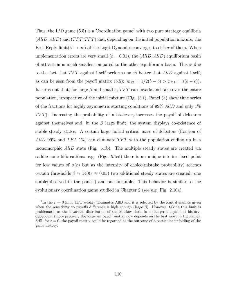
Thus, the IPD game (5.5) is a Coordination game7 with two pure strategy equilibria

(AllD;AllD) and (TFT; TFT ) and, depending on the initial population mixture, the

Best-Reply limit(� !1) of the Logit Dynamics converges to either of them. When

implementation errors are very small (" = 0:01), the (AllD;AllD) equilibrium basin

of attraction is much smaller compared to the other equilibrium basin. This is due

to the fact that TFT against itself performs much better that AllD against itself,

as can be seen from the payo¤ matrix (5.5): m22 = 1=2(b � c) > m11 = "(b � c)).

It turns out that, for large � and small "; TFT can invade and take over the entire

population, irrespective of the initial mixture (Fig. (5.1), Panel (a) show time series

of the fractions for highly asymmetric starting conditions of 99% AllD and only 1%

TFT ). Increasing the probability of mistakes ", increases the payo¤ of defectors

against themselves and, in the � large limit, the system displays co-existence of

stable steady states. A certain large initial critical mass of defectors (fraction of

AllD 99% and TFT 1%) can eliminate TFT with the population ending up in a

monomorphic AllD state (Fig. 5.1b). The multiple steady states are created via

saddle-node bifurcations: e.g. (Fig. 5.1cd) there is an unique interior �xed point

for low values of �(") but as the intensity of choice(mistake probability) reaches

certain thresholds � � 140(" � 0:05) two additional steady states are created: one

stable(observed in the panels) and one unstable. This behavior is similar to the

evolutionary coordination game studied in Chapter 2 (see e.g. Fig. 2.10a).

7In the " ! 0 limit TFT weakly dominates AllD and it is selected by the logit dynamics givenwhen the sensitivity to payo¤s di¤erence is high enough (large �). However, taking this limit isproblematic as the invariant distribution of the Markov chain is no longer unique, but history-dependent (more precisely the long-run payo¤ matrix now depends on the �rst move in the game).Still, for " = 0, the payo¤ matrix could be regarded as the outcome of a particular unfolding of thegame history.

110

0

0 . 2

0 . 4

0 . 6

0 . 8

1

1 . 2

0 5 1 0 1 5 2 0 2 5 3 0 3 5 4 0 4 5

A l l DT F T

(a) " = 0:01: Time series

0

0 . 2

0 . 4

0 . 6

0 . 8

1

1 . 2

0 5 1 0 1 5 2 0 2 5 3 0 3 5 4 0 4 5

A l l DT F T

(b) " = 0:05: Time series

(c) � = 200:Bifurcation diagram

(AllD; ")

(d) " = 0:05: Bifurcation diagram

(AllD; �)

Figure 5.1: Unconditional defectors (AllD) vs. Reciprocators (TFT). Di¤erent errors inthe implementation lead to di¤erent long-run steady states: a population of reciprocators(Panel (a)) or a population of defectors (Panel (b)). Panels (c)-(d) display co-existence ofstable steady states for large values of � and ". Remaining game parameters: b = 4; c =1; � = 200:

5.3.2 TFT vs. AllC

For an interaction between unconditional cooperators (AllC) and reciprocators (TFT )

the payo¤ matrix (5.3) reduces to:

24 TFT 12(b� c) b� c� b"+ 2c"� 2c"2

AllC b� c� 2b"+ c"+ 2b"2 (1� ") (b� c)

35 (5.6)

111

It is straightforward to see that, for small " and b > c we have:

b� c� 2b"+ c"+ 2b"2 >1

2(b� c)

b� c� b"+ 2c"� 2c"2 > (1� ") (b� c)

Consequently, the reduced 2 � 2 game (5.6) is of Hawk-Dove type and, thus, it has

three equilibria: two asymmetric in pure strategies (TFT;AllC) and (AllC; TFT )

and one symmetric in mixed strategies. The two asymmetric equilibria give rise

to a 2-cycle under best-reply dynamics (i.e. logit dynamics with large �) while

the interior equilibrium is unstable. A two-cycle, with population swinging back

and forth between the two asymmetric equilibria, is created via a period-doubling

bifurcation when either errors in implementation are small (Fig. 5.2c) or players

choose a best-reply (large �, Panel(d)). The intuition for the two-cycle relates to the

best-response correspondences in the payo¤ matrix above: TFT 2 BRfAllCgand

AllC 2 BRfTFTg. In the population game interpretation, when everyone plays

TFT (AllC) it is better to switch to AllC(TFT ). Still, the amplitude of the cycle

�uctuations varies with how responsive players are to payo¤ di¤erences, with the

full-scale two-cycle observed only for large �:

For intermediated values of " (e.g. " 2�14; 12

�for the b = 2; c = 1 game

parameterization)matrix (5.6) de�nes a dominance solvable (DS) game with (TFT; TFT )

as unique pure strategy equilibrium while for large " > 12the game is still dominance

solvable, but with (AllC;AllC) the unique equilibrium. The transition from a Hawk-

Dove to a Dominance Solvable structure in the space of 2� 2 games is illustrated in

Fig. 5.2ef for �nite and best-reply limit of �; respectively:

112

0

0 . 2

0 . 4

0 . 6

0 . 8

1

1 . 2

8 0 8 2 8 4 8 6 8 8 9 0 9 2 9 4

T F TA l l C

(a) small � = 15: Time series

0

0 . 2

0 . 4

0 . 6

0 . 8

1

1 . 2

8 0 8 2 8 4 8 6 8 8 9 0 9 2 9 4

T F TA l l C

(b) large � = 220: Time series

(c) � = 15: Bifurcation diagram

(TFT; ")


(TFT; �)

(e) � = 15: Game transition HD-DS (f) � = 100: Game transition HD-DS-DS

Figure 5.2: Reciprocators(TFT) vs Unconditional Cooperators(AllC). Time series of frac-tions of TFT and AllC players for small (Panel (a)) and large (Panel (b) intensity of choicevalues, respectively. Panels (c)-(d) display a period-doubling bifurcation with respect to" and �, leading to a 2-cycle. Last, Panels (e)-(f) show transition from a Hawk-Dove toDominance Solvable pattern. Game parameters: b = 2; c = 1; " = 0:01:

113

5.3.3 AllD vs. AllC

For a 2 � 2 ecology consisting of undiscriminating defective and cooperative types

the restricted payo¤ matrix reads:26664AllD AllC

AllD " (b� c) b� b"� c"

AllC b"� c+ c" (1� ") (b� c)

37775 (5.7)

We have:

" (b� c) > b"� c+ c"

b� b"� c" > (1� ") (b� c)

and the Iterated Prisoner�s Dilemma is a PD game itself with (AllD;AllD) as the

unique equilibrium. This case illustrates the standard prisoner�s dilemma argument:

unless errors in implementation are extremely high (e.g. " � 0:5 or � very small,

both making the players choice virtually random as in Fig. (5.3)a), the unconditional

cooperators are heavily exploited by defectors, a situation leading to full extinction

of the cooperative "trait" from the population (Fig. (5.3)b). The result is robust to

any initial mixture of the population. For small �nite � or relatively large mistake

probability there is a unique interior steady state of fractions (x�AllD; x�AllC) with x

�AllD

sliding towards 1 as � !1 and/or "! 0: Fig. (5.3)c-d illustrates the continuation

of the equilibrium with respect to each of the two parameters.

114

0 . 4

0 . 4 5

0 . 5

0 . 5 5

0 . 6

0 1 0 2 0 3 0 4 0 5 0

A l l DG T F T

(a) � = 0:05: Time series

0

0 . 2

0 . 4

0 . 6

0 . 8

1

1 . 2

0 5 1 0 1 5 2 0 2 5 3 0 3 5 4 0 4 5

A l l DA l l C



(AllD; ")


(AllD; �)

Figure 5.3: Unconditional defectors (AllD) vs. Unconditional cooperators(AllC). Unlessthe choice is almost random (Panel (a), � = 0:05), the system quickly converges to amonomorphic state with defectors only (Panel (b)). Unique steady state converging toan AllD population when � is large or " gets smaller (Panels (c)-(d)). Game parameters:b = 2; c = 1; " = 0:01:

5.3.4 AllD vs. GTFT

For a sub-ecology of undiscriminating defectors and generous reciprocators the game

matrix has the form:

115

26664AllD GTFT

AllD " (b� c) b"� c"� b"2 + bn� bn"

GTFT b"� c"+ c"2 � cn+ cn" nn+"

(b� c)

37775 (5.8)

which is always a coordination game for a �reasonable�IPD parameterization8.

This behaviors ecology generalizes the case discussed in subsection (5.3.1). Sim-

ilarly, the system displays co-existence of monomorphic steady states for the � !1

limit. Unlike the AllD vs. TFT case the multiplicity of steady states is preserved

even for very small " = 0:01 (Fig.5.4a-b) with AllD taking over the population

provided that it slightly outnumbers TFT in the initial mixture (Fig.5.4a). The

crucial parameter for this robust path-dependence, is the degree of generosity n

in GTFT strategy: "generous" TFT plays cooperate with quite large probability

(n = 0:3) even after the opponent defected and this makes it more prone to exploita-

tion from AllD compared to the typical TFT strategy. Reversing the initial mixture

leads to long-run behaviour qualitatively similar to the one observed in the AllD vs.

TFT sub-ecology (Fig.5.4b).

Panels (c)-(d) display the fold bifurcation scenarios through which the co-existing

monomorphic steady states emerge. For instance, in Panel (d) as the critical threshold

n � 0:3 is hit, a new stable �xed point is created with AllD players only for a

parameterization (" = 0:01; � = 200) for which uniqueness of the steady state was

observed in the AllD vs. TFT ecology. By carefully tuning in the generosity para-

meter in the GTFT strategy, one could generate co-existing stable steady states in

an AllD � (G)TFT ecology of repeated rules.

8AllD is a best reply to itself i¤ "2 + n"� n < 0 (satis�ed as long as n is an order higher than"); similarly, GTFT is best-response to itself as long as "2 + n"� n < 0 and b > c:

116

0

0 . 2

0 . 4

0 . 6

0 . 8

1

1 . 2

0 5 1 0 1 5 2 0 2 5 3 0 3 5 4 0 4 5

A l l DG T F T

(a) Initial mixture: AllD-60%,

GTFT-40%

0

0 . 2

0 . 4

0 . 6

0 . 8

1

1 . 2

0 5 1 0 1 5 2 0 2 5 3 0 3 5 4 0 4 5

A l l DG T F T

(b) Initial mixture: AllD-40%,

GTFT-60%

(c) " = 0:01; n = 0:3: Bifurcation

diagram (AllD; �)

(d) " = 0:01; � = 200: Bifurcation diagram

(AllD; n)

Figure 5.4: Unconditional defectors (AllD) vs. Generous reciprocators (GTFT). Long runbehavior strongly depends on the initial mixture of the population even for very small errorsin implementation. Panels (c)-(d): co-existence of monomorphic steady states(created viafold bifurcations) when n and � are large, even for tiny implementation errors ". Baselinegame parameters: b = 2; c = 1; " = 0:01; n = 0:3; � = 15:

5.3.5 AllD-WSLS

In this sub-case, the payo¤ matrix (5.3) reduces to :

24 AllD " (b� c) 12b� c"

WSLS b"� 12c (b� c) (1� 4"3 + 6"2 � 3")

35 (5.9)

117

For high enough bene�ts of cooperation (b > b�9), this payo¤ matrix represents a

Coordination game if:

" (b� c) > b"� 12c

(b� c)�1� 4"3 + 6"2 � 3"

�>1

2b� c"

In this case two pure strategy equilibria (AllD;AllD) and (WSLS;WSLS) exist.

One could notice �rst that, for small implementation errors ", Pavlov fares much

better against itself thanAllD does against itself ((b� c) (1� 4"3 + 6"2 � 3") > "(b�

c)): However, this may not be enough to o¤set the heavy exploitation Pavlov incurs

in mixed encounters when AllD gets, on average, half from the bene�ts lim"!0(12b� c")

while WSLS pays half of the costs lim"!0(b" � 1

2c): This situation is depicted in Fig.

(5.5)a where the population ends up in an all-defectors state. If, in addition to

small error probabilities, the bene�ts of cooperation are relatively large(b > b�); the

"own-type" interaction e¤ect may dominate the "cross" interaction e¤ect and the

whole population becomes entirely Pavlovian (Fig. 5.5b). However, this results is

dependent on the initial mixture of the population as for a given initial threshold of

AllD players, population cannot turn Pavlovian, irrespective of the relative size of

the bene�ts accrued to cooperation b:The co-existence of two stable, monomorphic

steady states for high bene�ts of cooperation is documented in Fig. 5.5c-d where

additional �xed points emerge as the parameters of interest -� and " respectively - are

changed. When bene�ts are low enough, b < b� the 2� 2 game becomes dominance

solvable (DS) with (AllD;AllD) the unique equilibrium. A bifurcation diagram with

respect to the bene�ts of cooperation b (Fig. 5.5e) reveals once the threshold b� is

passed, a transition in the space of 2 � 2 games from a Dominance Solvable game

with unique equilibrium to a Coordination game with two equilibria.

9b� = 2c(1� 2"+ 2"2)=(�4"+ 4"2 + 1)

118

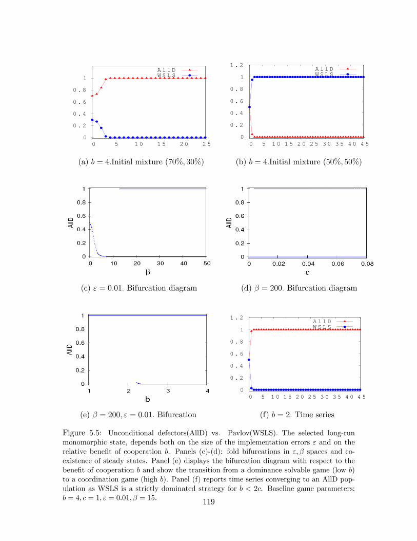
0

0 . 2

0 . 4

0 . 6

0 . 8

1

0 5 1 0 1 5 2 0 2 5

A l l DW S L S

(a) b = 4:Initial mixture (70%; 30%)

0

0 . 2

0 . 4

0 . 6

0 . 8

1

1 . 2

0 5 1 0 1 5 2 0 2 5 3 0 3 5 4 0 4 5

A l l DW S L S

(b) b = 4:Initial mixture (50%; 50%)

(c) " = 0:01: Bifurcation diagram (d) � = 200: Bifurcation diagram

(e) � = 200; " = 0:01: Bifurcation

0

0 . 2

0 . 4

0 . 6

0 . 8

1

1 . 2

0 5 1 0 1 5 2 0 2 5 3 0 3 5 4 0 4 5

A l l DW S L S

(f) b = 2: Time series

Figure 5.5: Unconditional defectors(AllD) vs. Pavlov(WSLS). The selected long-runmonomorphic state, depends both on the size of the implementation errors " and on therelative bene�t of cooperation b. Panels (c)-(d): fold bifurcations in "; � spaces and co-existence of steady states. Panel (e) displays the bifurcation diagram with respect to thebene�t of cooperation b and show the transition from a dominance solvable game (low b)to a coordination game (high b). Panel (f) reports time series converging to an AllD pop-ulation as WSLS is a strictly dominated strategy for b < 2c. Baseline game parameters:b = 4; c = 1; " = 0:01; � = 15: 119

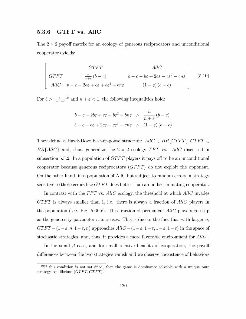
5.3.6 GTFT vs. AllC

The 2� 2 payo¤ matrix for an ecology of generous reciprocators and unconditional

cooperators yields:26664GTFT AllC

GTFT nn+"

(b� c) b� c� b"+ 2c"� c"2 � cn"

AllC b� c� 2b"+ c"+ b"2 + bn" (1� ") (b� c)

37775 (5.10)

For b > c1�n�"

10 and n+ " < 1; the following inequalities hold:

b� c� 2b"+ c"+ b"2 + bn" >n

n+ "(b� c)

b� c� b"+ 2c"� c"2 � cn" > (1� ") (b� c)

They de�ne a Hawk-Dove best-response structure: AllC 2 BRfGTFTg; GTFT 2

BRfAllCg and, thus, generalize the 2 � 2 ecology TFT vs. AllC discussed in

subsection 5.3.2. In a population of GTFT players it pays o¤ to be an unconditional

cooperator because generous reciprocators (GTFT ) do not exploit the opponent.

On the other hand, in a population of AllC but subject to random errors, a strategy

sensitive to those errors like GTFT does better than an undiscriminating cooperator.

In contrast with the TFT vs. AllC ecology, the threshold at which AllC invades

GTFT is always smaller than 1, i.e. there is always a fraction of AllC players in

the population (see. Fig. 5.6b-c). This fraction of permanent AllC players goes up

as the generosity parameter n increases. This is due to the fact that with larger n;

GTFT � (1�"; n; 1�"; n) approaches AllC� (1�"; 1�"; 1�"; 1�") in the space of

stochastic strategies, and, thus, it provides a more favorable environment for AllC .

In the small � case, and for small relative bene�ts of cooperation, the payo¤

di¤erences between the two strategies vanish and we observe coexistence of behaviors

10If this condition is not satisi�ed, then the game is dominance solvable with a unique purestrategy equilibrium (GTFT;GTFT ):

120

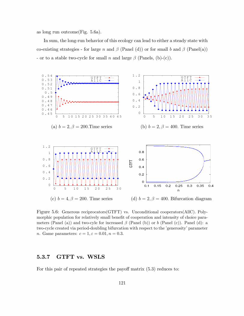
as long run outcome(Fig. 5.6a).

In sum, the long-run behavior of this ecology can lead to either a steady state with

co-existing strategies - for large n and � (Panel (d)) or for small b and � (Panel(a))

- or to a stable two-cycle for small n and large � (Panels, (b)-(c)).

0 . 4 5 0 . 4 6 0 . 4 7 0 . 4 8 0 . 4 9 0 . 5

0 . 5 1 0 . 5 2 0 . 5 3 0 . 5 4

0 5 1 0 1 5 2 0 2 5 3 0 3 5 4 0 4 5

G T F TA l l C

(a) b = 2; � = 200:Time series

0

0 . 2

0 . 4

0 . 6

0 . 8

1

1 . 2

0 5 1 0 1 5 2 0 2 5 3 0 3 5

G T F TA l l C

(b) b = 2; � = 400: Time series

0

0 . 2

0 . 4

0 . 6

0 . 8

1

1 . 2

0 5 1 0 1 5 2 0 2 5 3 0

G T F TA l l C

(c) b = 4; � = 200: Time series (d) b = 2; � = 400: Bifurcation diagram

Figure 5.6: Generous reciprocators(GTFT) vs. Unconditional cooperators(AllC). Poly-morphic population for relatively small bene�t of cooperation and intensity of choice para-meters (Panel (a)) and two-cyle for increased � (Panel (b)) or b (Panel (c)). Panel (d): atwo-cycle created via period-doubling bifurcation with respect to the �generosity�parametern. Game parameters: c = 1; " = 0:01; n = 0:3:

5.3.7 GTFT vs. WSLS

For this pair of repeated strategies the payo¤ matrix (5.3) reduces to:

121

24 GTFT nn+"

(b� c) m34

WSLS m43 (b� c) (1� 4"3 + 6"2 � 3")

35 (5.11)

where m43 and m34 are complicated expressions of all model parameters (see Ap-

pendix (5.A) for explicit formulas)). One can show, by algebraic manipulations, that

for n > "(by assumption):

n

n+ "(b� c) > m43

(b� c)�1� 4"3 + 6"2 � 3"

�> m34

and this 2� 2 ecology de�nes a Coordination game with two pure strategy, symmet-

ric Nash equilibria (GTFT;GTFT ) and (WSLS;WSLS). In the � large limit, the

equilibria structure of the coordination game describe the long-run behavior of the

logit dynamics. The corresponding basins of attraction relative sizes are signi�cantly

biased towards Pavlov players as it takes 70% of GTFT players in the initial pop-

ulation in order to converge to a log-run all GTFT state (Fig.5.7a), with anything

below this threshold reversing fortunes toward a long run Pavlov monomorphic state.

Intuitively, a stimulus-response, past-performance driven strategy like Pavlov, is able

to take advantage of the generosity built into GTFT which reverts, with large prob-

ability n; to "nice" behaviour after an opponent defection irrespective of the realized

history. This is because GTFT does not discriminate among possible causes of defec-

tion(be it after a DD, or a DC history), while Pavlov re-establishes cooperation only

after own defection. For �nite, small � the population converges to a unique �xed

point with co-existing behaviors of the form (x�GTFT ; x�WSLS); x

�GTFT + x

�WSLS = 1;

with Pavlov outnumbering generous reciprocators( x�WSLS slides up in the interval

[1=2; 1] as we increase �). Fig. 5.7c-d depict a saddle-node bifurcation route towards

co-existing monomorphic steady states. For low � (given n) or small n (�xing � close

to the "best-reply" limit) there is a unique polymorphic population steady state.

122

0

0 . 2

0 . 4

0 . 6

0 . 8

1

1 . 2

0 5 1 0 1 5 2 0 2 5 3 0

G T F TW S L S

(a) Time series, initial mixture 70%

GTFT-30% WSLS

0

0 . 2

0 . 4

0 . 6

0 . 8

1

1 . 2

0 5 1 0 1 5 2 0 2 5 3 0 3 5 4 0 4 5

G T F TW S L S

(b) Time series, initial mixture 50%

GTFT-50% WSLS

(c), n = 0:3: Bifurcation diagram

(WSLS; �)

(d) � = 100: Bifurcation diagram

(WSLS; n)

Figure 5.7: Generous reciprocators (GTFT) vs. Pavlovian(WSLS). Depending on theinitial fractions in the populations, in the � large limit, the system converges to a mono-morphic state with only one type of behavior surviving. Panels (c)-(d): creation of twoco-existing steady states via a fold bifurcation when the degree of generosity/intensity ofchoice is varied. Game parameters: b = 4; c = 1; " = 0:01; n = 0:3; � = 100:

123

5.3.8 TFT vs. GTFT

For a population of generous and standard tit-for-tatters, the payo¤ matrix has the

form: 26664TFT GTFT

TFT 12b� 1

2c � c"�b"+b"2�bn+cn+bn"�2cn"

n+3"�2n"�2"2

GTFT b"�c"+c"2+bn�cn�2bn"+cn"n+3"�2n"�2"2

nn+"

(b� c)

37775 (5.12)

For n > ", straightforward manipulations show that:

b"� c"+ c"2 + bn� cn� 2bn"+ cn"n+ 3"� 2n"� 2"2 >

1

2b� 1

2c, b > b�� =

c

1� n� "n

n+ "(b� c) > �c"� b"+ b"

2 � bn+ cn+ bn"� 2cn"n+ 3"� 2n"� 2"2 , b > b� =

c

1� 2"

So, for b > b�� the game is dominance solvable with (GTFT;GTFT ) as the unique

Nash equilibrium11. Consequently, in the � ! 1 limit , the fraction of GTFT

players converges to 1 as there is no selection pressure against a more "generous"

reciprocative type as long as the rest of the population proceeds to a mimicking

behavior. GTFT is a generalization of TFT and a population of TFT provides a

stepstone for "nicer" behaviour to �ourish. The lack of strongly defective players

creates a payo¤ advantage for GTFT , inducing more switching away from TFT ,

with population eventually ending up in an all GTFT state (Fig. 5.8a).

For b 2 (b�; b��) the best responses are TFT 2 BRfTFTg; GTFT 2 BRfGTFTg

and we are in the case of a Coordination game with Logit Dynamics displaying

co-existence of behavioral rules, but with GTFT largely outnumbering TFT (Fig.

5.8b).

The transition in the space of 2�2 games is illustrated by the bifurcation diagram

11similarly, if b 2 (b�; b��) then we have a coordination game while for b < b� the game is againdominance solvable, with (TFT; TFT ) unique pure-strategy Nash equilibrium.

124

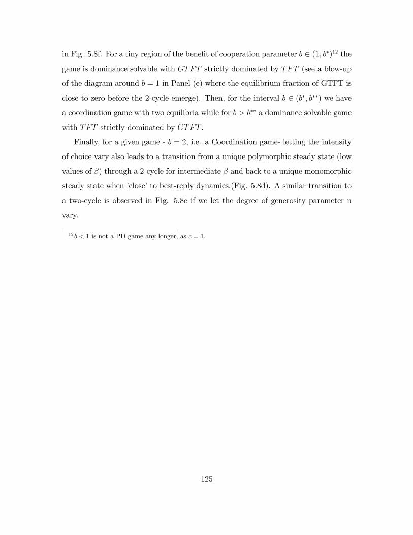
in Fig. 5.8f. For a tiny region of the bene�t of cooperation parameter b 2 (1; b�)12 the

game is dominance solvable with GTFT strictly dominated by TFT (see a blow-up

of the diagram around b = 1 in Panel (e) where the equilibrium fraction of GTFT is

close to zero before the 2-cycle emerge). Then, for the interval b 2 (b�; b��) we have

a coordination game with two equilibria while for b > b�� a dominance solvable game

with TFT strictly dominated by GTFT .

Finally, for a given game - b = 2, i.e. a Coordination game- letting the intensity

of choice vary also leads to a transition from a unique polymorphic steady state (low

values of �) through a 2-cycle for intermediate � and back to a unique monomorphic

steady state when �close�to best-reply dynamics.(Fig. 5.8d). A similar transition to

a two-cycle is observed in Fig. 5.8e if we let the degree of generosity parameter n

vary.

12b < 1 is not a PD game any longer, as c = 1.

125

0

0.2

0.4

0.6

0.8

1

1.2

0 5 10 15 20

TFTGTFT

(a) b = 2; � = 700: Time series

0

0.2

0.4

0.6

0.8

1

1.2

0 5 10 15 20 25 30 35 40 45

TFTGTFT

(a) b = 1:5; � = 700: Time series

(c) b = 2. Bifurcation diagram (GTFT,n) (d) b = 2. Bifurcation diagram (GTFT,�)

(e) � = 1000: Game transition DS-HD (f) � = 700: Game transition DS-HD-DS

Figure 5.8: Reciprocators(TFT) vs. Generous reciprocators(GTFT). This ecology givesrise to a dominance solvable game for relatively large bene�ts of cooperation (Panel (a)) andto a Coordination game for intermediate values (Panel (b)). For a �xed Coordination game,Panel (d) shows the transition from a unique polymorphic steady state to a 2-cycle and backto a monomorphic steady state. In Panels (e)-(f) the transition in the space of 2 x 2 games isillustrated for the � large limit. Game parameters: b = 2; c = 1; " = 0:01; n = 0:3; � = 700:

126

5.3.9 TFT vs. WSLS

For this ecology of strategies the payo¤ matrix (5.3) boils down to:

26664TFT WSLS

TFT 12b� 1

2c 1

2b� 1

2c

WSLS 12b� 1

2c (b� c) (1� 4"3 + 6"2 � 3")

37775 (5.13)

For small implementation errors "; WSLS weakly dominates TFT and, in the

large � limit, Logit Dynamics leads to elimination of weakly dominated strategies

(Fig. 5.9a). Intuition draws on Pavlov essentially being a performance-dependent

strategy (i.e. change status-quo when unsatis�ed with the past period payo¤) relative

to TFT�s merely mimicking opponent past move.

For smaller � the payo¤ di¤erential between the two strategies is small and the

system converges to a steady state with co-existing rules (Fig. 5.9b).

0

0 . 2

0 . 4

0 . 6

0 . 8

1

1 . 2

0 5 1 0 1 5 2 0 2 5 3 0 3 5 4 0 4 5

T F TW S L S


0

0 . 2

0 . 4

0 . 6

0 . 8

1

0 5 1 0 1 5 2 0

T F TW S L S


Figure 5.9: Reciprocators (TFT) vs. Pavlov(WSLS). Panel (a): large values of the intens-ity of choice, quick convergence to monomorphic population consisting only of Pavlovianplayers, irrespective of the cooperation bene�ts size b. Panel (b) shows convergence to apolymorphic state for low �. Game parameters: b = 2; c = 1; " = 0:01; n = 0:3; � = 100:

127

5.3.10 WSLS vs. AllC

The payo¤ matrix for this ecology reads:26664WSLS AllC

WSLS (1� ")(1� 2"+ 4"2)(b� c) b� 12c� b"

AllC b� c� 2b"+ c"+ 2b"2 (1� ")(b� c)

37775 (5.14)

If b > b�13 the game (5.14) is of Hawk-Dove type with two asymmetric pure

strategy equilibria (AllC;WSLS) and (WSLS;AllC) and one , interior equilibrium,

in mixed strategies. One could notice that, in the " ! 0 limit, Pavlov and AllC

perform equally well against their own type but Pavlov does relatively better in a

mixed matching (b� 12c > b�c): However for strictly positive errors, AllC does better

against its own type than Pavlov ((1� 2"+ 4"2) < 1). This gives a payo¤ advantage

for AllC which ensures that it does not go extinct but survives in small fractions

subjected to perpetual oscillations (Fig. 5.10)a). For a given game matrix, the

two-cycle is created, as usual, via a period-doubling bifurcation when, for instance,

the intensity of choice � is increased (Fig. 5.10d). Panel (c) in Fig. 5.10 displays

the transition, in the 2 � 2 games space, from a dominance solvable (low b) to a

Hawk-Dove game (large b). The logit dynamics attracting set shifts from a unique

monomorphic steady state with Pavlov players only to a 2-cycle alternating between

WSLS and AllC:

13b� = 2c 1�"1�2" � 2c: Otherwise, the game is dominance solvable withWSLS surviving eliminationof strictly dominated AllC:

128

0

0 . 2

0 . 4

0 . 6

0 . 8

1

1 . 2

0 5 1 0 1 5 2 0

W S L SA l l C


0

0 . 2

0 . 4

0 . 6

0 . 8

1

1 . 2

0 5 1 0 1 5 2 0

W S L SA l l C



(WSLS; b)

(d) b = 2: Bifurcation diagram

(WSLS; �)

Figure 5.10: Pavlov (WSLS) vs. Unconditional cooperators (AllC). Oscillatory co-existence of strategies with Pavlovian behaviour outnumbering unconditional cooperatorsfor small intensity of choice (Panel (a)) and continuous swings between monomorphic stateswhen � approaches the �best respose" limit (Panel (b)). Panel (c) illustrates the bifurca-tion in the space of games, as the bene�t of cooperation varies, from a unique steady state(equilibrium) to a 2-cyle (2 asymmetric equilibria). Panel (d): as the intensity of choiceincreases the long-run outcome changes from a polymorphic steady state to a 2-cycle.Remaining game parameters: b = 2; c = 1; " = 0:01; n = 0:3; � = 15:

129

5.3.11 Summary

Table 5.1 summarizes the normal form games resulting from 10 di¤erent the strategic

pairwise interaction of the �ve repeated PD strategies together with the long-run

attractors of the corresponding evolutionary game under the perturbed best-reply

dynamics. In the limiting � ! 1 case, these long-run outcomes coincide with the

attracting sets of the unperturbed best-reply dynamics on the respective 2�2 game.

No. 2x2 Game Bifurcation Attractors Path-

� large Dependence

1 AllD-TFT WDS,C SN multiple SS yes, " = 0:05

2 TFT-AllC HD PD 2-cycle no

3 AllD-AllC DS none unique SS no

4 AllD-GTFT C SN multiple SS yes, " = 0:01

5 AllD-WSLS DS,C SN multiple SS yes, b = 4

6 GTFT-AllC HD PD 2-cycle yes

7 GTFT-WSLS C SN multiple SS yes

8 TFT-GTFT DS, C PD 2-cycle no

9 TFT-WSLS WDS none unique SS no

10 WSLS-AllC DS,HD PD 2-cycle no

Table 5.1: Summary of the type of game and dynamical behaviour for all 10 pairwiseinteraction of iterated Prisoner�s Dilemma strategies under logit dynamics.

We have encountered the following typical pairwise interactions between iter-

ated Prisoner�s Dilemma strategies together with transition from one game form to

another as the payo¤ matrix parameters (b; c; "; n) change:

� Coordination game (C): multiplicity of monomorphic(only one type of beha-

viour surviving) steady states with strong path-dependence

� Hawk-Dove game (HD): asymmetric equilibria; 2-cycle with continuous popu-

130

lation switching from one monomorphic state to the other

� Prisoner�s Dilemma (PD): uniquely selected long run symmetric, Pareto-inferior,

equilibrium (i.e. monomorphic population state)

� Dominance Solvable game (DS), non-PD : unique, monomorphic long-run steady

state

� Games with a weakly dominated strategy (WDS): unique, monomorphic long-

run steady state

The co-existing steady states and 2-cycles emerging under logit dynamics are

usually created via fold/ saddle-node (SN) and period-doubling (PD) bifurcations,

respectively. Although the qualitative changes in the space of 2 � 2 games do not

make the object of the present chapter, some interesting game transitions were also

revealed and it would be worth studying them systematically, as future research.

131

5.4 3�3 Ecologies

In this section we will discuss some typical examples out of the

0@ 5

3

1A = 10 sub-

ecologies of three iterated PD strategies, focusing the analysis on the resulting 3� 3

normal form games and on the attracting sets and long-run behavior of the logit

evolutionary dynamics.

5.4.1 AllD-TFT-AllC

This ecology has been thoroughly investigated in Sigmund and Brandt (2006) under

the Replicator Dynamics. The reduced 3� 3 payo¤ matrix reads:26666664AllD TFT AllC

AllD " (b� c) �" (c� 2b+ 2b") b� b"� c"

TFT " (b� 2c+ 2c") 12b� 1

2c b� c� b"+ 2c"� 2c"2

AllC b"� c+ c" b� c� 2b"+ c"+ 2b"2 (1� ") (b� c)

37777775(5.15)

After normalization (all elements on the main diagonal set equal to zero by, for

instance, deducting the diagonal entry from each column for player I/or from each

row for player II) we get:

26666664AllD TFT AllC

AllD 0 12(1� 2") (c� b+ 2b") c (1� 2")

TFT �c" (1� 2") 0 c" (1� 2")

AllC c (2"� 1) 12(1� 2") (b� c+ 2b") 0

37777775As 1

2(1� 2") (c� b+ 2b") < 0 and c (1� 2") > 0 this matrix has, in the "! 0

limit, a generalized Rock-Paper-Scissors structure14. Namely, AllD ties with its own

14Sigmund and Brandt (2006) also discover, when mistakes probability " ! 0, a RSP patternunder Replicator Dynamics, for a similar ecology of IPD game rules, with discounting.

132

type, loses to TFT and wins at AllC.

Putting together insights from subsections (5.3.1), (5.3.2) and (5.3.3) we notice

that, in a stochastic strategy framework, for "! 0; this ecology resembles very much

a Rock-Paper-Scissors pattern of behavior: each of the three repeated strategies

provide the environment in which another one can emerge and take over in the fol-

lowing order: a population of unconditional defectors (AllD) is prone to invasion and

supersession by small clusters of reciprocators (TFT ) which, upon reaching a crit-

ical threshold, provide the stepstone for the emergence of unconditional cooperators

(AllC). These AllC players grow in the population up to the limit when conditions

are created for unconditional defectors (AllD) to thrive, strike back in the popula-

tion and, thus, complete the full cycle (see Fig. 5.11e). Any small number of AllD

players is able to invade a population of AllC given that AllD strongly dominates

AllC (from subsection (5.3.3)) while, in fact, TFT can never invade a population

of unconditional cooperators (subsection (5.3.2)). Fig. 5.11c-d depict projections of

one such invariant curve onto subspaces of two strategies, together with the Hopf bi-

furcation route to periodic behavior (see Panels (a),(b), (f) for bifurcation diagrams

of AllD and TFT fractions varying the bene�t of cooperation b, mistake probability

" and intensity of choice � parameters, respectively). The limit cycles born at �nite

values of � turn into a 3-cycle in the vanishing errors and "best-response" limits

"! 0; � !1; according to the best-reply structure of the underlying RSP game.

133

(a) " = 0:01:Bifurcation diagram (b) b = 2. Bifurcation diagram

(c) b = 1:4984: Phase plot (d) b = 1:4984: Phase plot

0

0.2

0.4

0.6

0.8

1

1.2

0 2 4 6 8 10 12 14

AllDTFT

AllC

(e) � = 100: Time series (f) b = 2. Bifurcation diagram

Figure 5.11: AllD vs. TFT vs. AllC. Bifurcation diagrams with respect to the bene�tof cooperation parameter b (Panel (a)), probability of mistake (Panel (b)) and intensityof choice (Panel (f)). Panels (c)-(d): phase plots in AllD-TFT and TFT-AllC subspaces,displaying Rock-Paper-Scissors type of long-run behaviour. Last, Panel (e) shows fractionsevolution for large �. Baseline game parameters: b = 2; c = 1; " = 0:01; n = 0:3; � = 10:

134

5.4.2 AllD-GTFT-WSLS

The 3x3 payo¤ matrix reads:26666664AllD GTFT WSLS

AllD " (b� c) m1312b� c"

GTFT m31nn+"

(b� c) m34

WSLS b"� 12c m43 (b� c) (1� 4"3 + 6"2 � 3")

37777775 (5.16)

With the help of the pairwise payo¤ comparisons15 performed in subsections (5.3.4),

(5.3.5) and (5.3.7), given n > " (by assumption), we can easily derive the best-

response correspondences in game form (5.16) as follows: fAllDg = BRfAllDg,

fGTFTg = BRfGTFTg and fWSLSg = BRfWSLSg. Thus, the game is a 3� 3

coordination game, and, in the best-reply limit of our logit dynamic(i.e. � ! 1)

each of these three pure strategy symmetric equilibria could be obtained as long-run

outcome if the population starts out with the appropriate distribution of fractions.

See Fig.5.12f for a set of initial conditions from which the (WSLS;WSLS) is selected.

For � �nite, the situation becomes more intricate as the Logit dynamics appear to

break the typical coordination game best-response structure described above and

generate Rock-Paper-Scissors patterns of cyclical oscillations irrespective of the initial

mixture of the population (Fig.5.12a-d).

As the bifurcation diagram with respect to � (Fig.5.12e) suggests, a unique, fully

mixed steady state for low values, destabilizes, for moderate values of the intensity

of choice, via a Neimark-Sacker (NS) bifurcation, and RSP-like stable, limit cycles

appear. For high values of � a sequence of saddle-node (SN) bifurcations occurs,

conducing to three16 co-existing stable steady states, in the � ! 1 limit. This

bifurcation scenario is con�rmed in Fig. 5.13 where we continue a barycentrical �xed

15 i.e. the best-response functions for the corresponing 2� 2 games.16Panel (e) displays, for large � only two values of Pavlov fractions steady states, the top one

with 100% share of WSLS and the bottom one with 0%. The third steady state supersedes thebottom curve, with zero WSLS fraction, too.

135

point (1=3; 1=3; 1=3)) in the bene�t of cooperation/error in strategy execution space

(top panels) and detect the conjectured Neimark-Sacker (NS)-Period-Doubling (PD)-

Saddle-Node (LP) sequence of bifurcations along the equilibrium curve. The middle

and bottom panels of Fig. 5.13 �continue�each detected codimension I singularity

with respect to another game or behavioral parameter and displays the resulting

bifurcation curves .When a NS/PD/LP curve of codimension I bifurcations is crossed

from below a limit cycle/2-cycle/co-existing stable and unstable steady states emerge,

respectively. Also, it is worthwhile pointing out the rich selection of codimension II

bifurcations occurring along the curves of codimension I bifurcations in this 3x3

ecology of repeated Prisoner�s Dilemma rules under the Logit Dynamics.

The intuition for the emergence, within a Coordination game, of the Rock-Paper-

Scissors cycles "GTFT beats AllD, WSLS beats GTFT and AllD beats WSLS"

is not immediately clear. We know that in the � ! 1 limit the interaction is of

Coordination game type with the three co-existing stable steady states created via

a sequence of saddle-node bifurcations as shown before. Still, for �nite values of the

intensity of choice � (Fig.5.12e) the typical Coordination game (each strategy Ei is

a best-reply to itself) behaves dynamically as if a RSP game (each strategy Ei is

a best reply to its successor Ei+1): Nevertheless, even for �nite � the Coordination

game dynamic behavior can be recovered if the bene�ts accrued to cooperation b are

high enough (Fig.5.12a).

136

(a) � = 15: Bifurcation diagram, b (b) � = 15: Bifurcation diagram, "

(c) b = 2:16:Phase plot

0

0 . 2

0 . 4

0 . 6

0 . 8

1

1 . 2

4 0 5 0 6 0 7 0 8 0 9 0

A l l DG T F T

P a v l o v

(d) b = 2:16: Time series

(e) b = 2:2. Bifurcation diagram

0

0 . 2

0 . 4

0 . 6

0 . 8

1

1 . 2

0 2 4 6 8 1 0

A l l DG T F TW S L S

(f) � = 100: Initial fractions (0.2,0.3,0.5)

Figure 5.12: AllD vs. GTFT vs. WSLS. Bifurcation diagrams with respect to the bene�tof cooperation parameter b (Panel (a)) and probability of mistakes (Panel (b)). Phaseplots in GTFT-WSLS space (Panel (c)) and time series (Panel (d)), displaying Rock-Paper-Scissors type of long-run behaviour for moderate �. Bifurcation diagram with respect to� and time series (Panel (f)) showing convergence, in the � large limit to the all Pavlovsteady state(for an approapriate initial population mixture). Baseline game parameters:b = 2; c = 1; " = 0:01; n = 0:1; � = 15:

137

1 2 3 40

0.2

0.4

0.6

0.8

1 LP

LPNS

NS

PD

b

AllD

0.05 0.03 0.01 0.01 0.03 0.050

0.2

0.4

0.6

0.8

1

LPNS

PD

PDLP

NS

PD

ε

AllD

0.05 0 0.05 0.1 0.15 0.21.5

2

2.5

3

3.5

4

R1

CP

R1

LPPD

CP

R1

R1

ε

bene

fit o

f coo

pera

tion

b

LPPD

GPD

LP

NSPD

PDLP

NS

0 5 10 15 201

1.5

2

2.5

3

3.5

4

R1

R1CP

CP

LPPD

GPD

β

bene

fit o

f coo

pera

tion

b

LPPDLP

LPNS

NS

PDLPLPPD

0 0.2 0.4 0.61

2

3

4

5

6

CP

R1

R1

CH R1

n

bene

fit o

f coo

pera

tion

b

LP

LP

NS

NS

5 10 15 200.02

0

0.02

0.040.04

R1CP

β

ε

LP

NS

NS

LP

PD

PD

Figure 5.13: AllD vs. GTFT vs. WSLS. Top panels: continuation of an equilibriumin the bene�t of cooperation and error probability space. Middle and bottom panels:continuation of the Period-Doubling (PD), Saddle-Node (LP) and Neimark-Sacker (NS)singularities detected in the top two panels with respect to a second parameter: intensityof choice �, degree of generosity n, bene�t of cooperation b and error in implementation �.Baseline game parameters: b = 2; c = 1; " = 0:01; n = 0:1; � = 15:

138

5.4.3 AllD-GTFT-AllC

The restriction of the full payo¤ matrix (5.3) to this 3 � 3 sub-ecology, can be

arranged, after the normalization of diagonal payo¤s into the following form:26666664AllD GTFT AllC

AllD 0 � 1n+"

(n� "2 � n") (b� c� bn� b") c (1� 2")

GTFT �c (n� "2 � n") 0 c" (1� n� ")

AllC �c (1� 2") "n+"

(1� n� ") (b� c� bn� b") 0

37777775(5.17)

It is easy to see that, for "; n ! 0 this normalized payo¤ matrix has a general-

ized Rock-Paper-Scissors structure, i.e. AllD outcompetes AllC, AllC outcompetes

GTFT and GTFT outcompetes AllD. In this case the logit dynamics has a limit

cycle as an attracting set for moderate � and a three cycle with perpetual switch-

ing between the three monomorphic steady states in the � large limit. For strictly

positive perturbations "; n the game is not RSP per se but, nevertheless, the Logit

Dynamics generates, for low to intermediate values of the intensity of choice, peri-

odic behavior resembling the described RSP cycles. Reasoning for the emergence of

such limit cycles in Fig. 5.14c-d goes along the best-reply correspondences argument

already sketched in subsection (5.4.1). Unlike the AllD � TFT � AllC ecology, the

shape of the curve, as well as the oscillations bounds, are distorted, with the ori-

ginal ones recovered in the limit n! " when GTFT approaches the TFT strategy.

However, in the � !1 limit system converges to a monomorphic AllD state (Fig.

5.14e-f). The presence of undiscriminating cooperators leads to the extinction of the

generous reciprocators.

139

(a) n = 0: _2: Bifurcation diagram (b) " = 0:01: Bifurcation diagram

(c) b = 1:72: Phase plot

0

0 . 2

0 . 4

0 . 6

0 . 8

1

1 . 2

5 0 5 5 6 0 6 5 7 0 7 5 8 0 8 5 9 0

A l l DG T F TA l l C

(d) b = 1:72: Time series

(e) " = 0:01: Bifurcation diagram

0

0 . 2

0 . 4

0 . 6

0 . 8

1

1 . 2

0 2 4 6 8 1 0

A l l DG T F TA l l C

(f) � = 100: Time series

Figure 5.14: AllD vs. GTFT vs. AllC. Bifurcation diagrams with respect to the bene�tof cooperation parameter b (Panel (a)) and degree of generosity n (Panel (b)). Phase plotsin AllC-GTFT space together with Rock-Paper-Scissors time series are reported in Panels(c) and (d), respectively. Panels (e),(f) display the long run behaviour in the � large limit.Baseline game parameters: b = 2; c = 1; " = 0:01; n = 0:1; � = 15;

140

5.4.4 AllD-TFT-WSLS

The payo¤ matrix for this sub-ecology takes the following form:26666664AllD TFT WSLS

AllD 0�12� "�(c� b+ 2b")

�"� 1

2

�(b� 2c� 4b"+ 4c"+ 4b"2 � 4c"2)

TFT c" (2"� 1) 0 12(b� c) (2"� 1)3

WSLS c�"� 1

2

�0 0

37777775(5.18)

which, in the limit "! 0; simpli�es to:

26666664AllD TFT WSLS

0 �12(b� c) c� 1

2b

0 0 �12(b� c)

�12c 0 0

37777775For relatively small bene�ts of cooperation (c < b � 2c) we see that AllD loses to

TFT (�12� "�(c� b+ 2b") < 0): Unconditional defectors AllD win against WSLS

(�"� 1

2

�(b� 2c� 4b"+ 4c"+ 4b"2 � 4c"2) > 0) and tie against own-type. Thus, this

matrix has a degenerate generalized Rock-Paper-Scissors structure and limit cycles

are born via a Hopf bifurcation, for low17 to moderate values of the intensity of choice

parameter � (Fig. 5.15a-d) with a 3-cycle arising in the � ! 1 limit. For strictly

positive mistake probability " there are still RPS cycles born, but only for moderate

values of the intensity of choice, while, for large intensity of choice, the population

ends up in an AllD monomorphism (Panel(e)). The intuition for these oscillations

could be extracted from results derived in subsections (5.3.1), (5.3.5) and (5.3.9): for

small errors of implementation TFT weakly dominates AllD, in turn, is it weakly

dominated by WSLS and, �nally, AllD easily invades a Pavlovian population when

bene�ts accrued to cooperation are small (see Fig. 5.5a). For strictly positive " and

17If � = 0; the repeated strategy choice is random and the unique steady state is the fully mixedpopulation state.

141

� !1 the population converges to an AllD monomorphic state.

If the relative bene�ts are large (b > 2c), the RSP structure disappears for " !

0, and, for � large the population converges, irrespective of the initial mixture, to

a Pavlov-only state (Panel (f)). Notice that, even if the underlying game itself is

no longer RSP, there are still oscillations for moderate � due to the evolutionary

dynamics.

142

(a) n = 0:2: Bifurcation diagram, b (b) n = 0:2: Bifurcation diagram, "

(c) b = 2:16: Phase plot

0

0 . 2

0 . 4

0 . 6

0 . 8

1

4 0 4 5 5 0 5 5 6 0 6 5 7 0

A l l DT F T

W S L S

(d) b = 2:16:Time series

(e) b � 2 _c: Bifurcation diagram (f) b > 2 _c: Bifurcation diagram

Figure 5.15: AllD vs. TFT vs. WSLS. Bifurcation diagrams with respect to the bene�t ofcooperation parameter b (Panel (a)) and probability of mistakes (Panel (b)). Phase plots inAllD-WSLS (Panel (c)) and time series (Panel (d)) displaying Rock-Paper-Scissors type oflong-run behaviour. Panels (e)-(f) show long-run behavior and convergence, for large �, toAllD (Pavlov) monomorphism for b < 2c (b > 2c, respectively). Baseline game parameters:b = 2; c = 1; " = 0:01; n = 0:2; � = 15;

143

5.4.5 AllD-TFT-GTFT

The reduced 3 � 3 payo¤ matrix for an ecology of defectors and (generous) recip-

rocators reads:26666664AllD TFT GTFT

" (b� c) �" (c� 2b+ 2b") b"� c"� b"2 + bn� bn"

" (b� 2c+ 2c") 12b� 1


n+3"�2n"�2"2

b"� c"+ c"2 � cn+ cn" b"�c"+c"2+bn�cn�2bn"+cn"n+3"�2n"�2"2

nn+"

(b� c)

37777775(5.19)

Using the inequalities from the relevant 2� 2 sub-ecologies (subsections (5.3.1),

(5.3.4) and (5.3.8)) we can show that, for b > c1�n ; there are only two pure strategy

equilibria (AllD;AllD) and (GTFT;GTFT ). By adding the GTFT strategy to the

coordination game AllD vs. TFT in (5.3.1), the steady state (TFT; TFT ) is lost.

However, TFT is not a dominated strategy and it plays an �intermediate layer�role

in ensuring transition from AllD to GTFT . Moreover, for small "; TFT breaks the

path-dependence observed in the AllD vs. GTFT ecology (see subsection (5.3.4))

and, in the � !1 limit; (GTFT;GTFT ) is the unique steady state (Fig. 5.16b,f).

The intuition relies on the fact that there are only two possible transitions leading to

an GTFT�only population: from TFT to GTFT (�immediate�in the � large case as

TFT is strictly dominated strategy) and from AllD to GTFT (in two stages): in the

�rst stage TFT (unlike GTFT ) invades and supersedes AllD for any initial fraction

of defectors while in the second stage GTFT supersedes TFT according to the

strict dominance criterion. Interestingly, for relatively small bene�t of cooperation18,

oscillatory co-existence of all three strategies (Fig. 5.16c-d) is observed for moderate

�; while for � !1 population converges to an AllD state.

18Actually, the normalized game matrix in the "! 0 limit, is

24 0 12c�

12b c� b+ bn

0 0 0�cn 1

2b�12c 0

35 ; adegenerate Rock-Paper-Scissors for c < b < c

1�n :

144

0

0 . 2

0 . 4

0 . 6

0 . 8

1

1 . 2

1 0 0 1 0 5 1 1 0 1 1 5 1 2 0

A l l DT F T

G T F T

(a) b = 3; � = 25: Time series

0

0 . 2

0 . 4

0 . 6

0 . 8

1

1 . 2

0 5 1 0 1 5 2 0

A l l DT F T

G T F T

(b) b = 3; � = 300: Time series

(c) b = 1:2; � = 29:8: Limit cycle

0

0 . 2

0 . 4

0 . 6

0 . 8

1

1 . 2

0 5 1 0 1 5 2 0

A l l DT F T

G T F T

(d) b = 1:2; � = 300: 5-cycle

(e) b < c=(1� n): Bifurcation diagram (f) b > c=(1� n): Bifurcation diagram

Figure 5.16: AllD vs. TFT vs. GTFT. Panels (a)-(d): Evolution of strategies fractions forsmall and large bene�t of cooperation coupled with low and high values of the sensitivity topayo¤ di¤erences, respectively. Remaning (game) parameters set to: c = 1; " = 0:01; n =0:3:

145

5.4.6 AllD-WSLS-AllC

The reduced 3� 3 payo¤ matrix for an ecology of defective, stimulus-response and

cooperative players takes the following form:26666664AllD WSLS AllC

AllD " (b� c) 12b� c" b� b"� c"

WSLS b"� 12c (b� c) (1� 4"3 + 6"2 � 3") b� 1

2c� b"

AllC b"� c+ c" b� c� 2b"+ c"+ 2b"2 (1� ") (b� c)

37777775 (5.20)

We notice �rst, that AllC is strictly dominated by WSLS provided that b <

2c 1�"1�2" ; the necessary and su¢ cient condition for Pavlov to be a best-reply to itself:

In this case the equilibria structure is given by the equilibria of the AllD vs. WSLS

game - (AllD;AllD) and (WSLS;WSLS) - in subsection (5.3.5). But, in the limit

"! 0; the ecology AllD�WSLS was dominance solvable for b < 2 _c withWSLS the

strictly dominated strategy. Combining the two restrictions, we obtain (AllD;AllD)

as the only remaining Nash equilibrium in our 3x3 ecology for small bene�ts of

cooperation b < 2c:

If b > 2c 1�"1�2" ; then AllC is a best-reply to WSLS; but WSLS is not a best reply

to AllC (as b � b" � c" > b � 12c � b") so both the Coordination and the Hawk-

Dove patterns of the AllD �WSLS and WSLS � AllC ecologies (see subsection

(5.3.10) are broken. Again we are only left with (AllD;AllD) as the unique pure

strategy equilibrium.(Fig. 5.17a). We observe the same phenomenon as with the

AllD � GFTF � AllC ecology, i.e. the presence of undiscriminating players AllC

leads to the extinction of the discriminating type Pavlov.

Interestingly, if we relax the � ! 1 assumption, the logit dynamics easily gen-

erates periodic (Fig. 5.17b-c) or chaotic behavior with irregular switching between

the three strategies. Fig. (5.17d) shows a plot of the largest Lyapunov exponent

�, with � > 0 implying chaos. In this case complicated dynamics arises through a

period-doubling route to chaos.

146

0

0 . 2

0 . 4

0 . 6

0 . 8

1

1 . 2

0 5 1 0 1 5 2 0

A l l DW S L SA l l C

(a) b > 2c; � = 300: Time series

0

0 . 2

0 . 4

0 . 6

0 . 8

1

1 . 2

1 0 0 1 0 5 1 1 0 1 1 5 1 2 0

A l l DW S L SA l l C

(b) b > 2c; � = 30. Time series


10.80.60.40.2

0 0.2 0.4 0.6

3.5 4 4.5 5 5.5 6

Lyapunov exp.

b

(d) � = 30:Largest Lyapunov exponent

(e) b = 4:4: Bifurcation diagram

1

0 . 5

0

0 . 5

1

2 0 2 5 3 0 3 5 4 0

Lyapunov exp.

β

(f) b = 4:4: Largest Lyapunov exponent

Figure 5.17: AllD vs. WSLS vs. AllC. Time series evolution for small and high values of �(Panels (a)-(b). Bifurcation diagram with respect to the bene�t of cooperation b (intensityof choice �) and evidence for chaotic behavior in Panels (c)-(d) and (e)-(f), respectively.Game parameters: b = 4; c = 1; " = 0:01; n = 0:3:

147

5.4.7 TFT-WSLS-AllC

The 3� 3 payo¤ matrix for an ecology of reciprocators, Pavlovians and cooperators

is given by:26666664TFT WSLS AllC

12b� 1

2c 1

2b� 1

2c b� c� b"+ 2c"� 2c"2

12b� 1

2c (b� c) (1� 4"3 + 6"2 � 3") b� 1

2c� b"

b� c� 2b"+ c"+ 2b"2 b� c� 2b"+ c"+ 2b"2 (1� ") (b� c)

37777775(5.21)

By comparing entries in this payo¤ matrix, we notice the best-reply correspond-

ences: fAllCg = BRfTFTg; fWSLSg = BRfAllCg. Also, fAllCg = BRfWSLSg

for b > 2c and fWSLSg = BRfWSLSg if b < 2c. Consequently, apart from mixed

strategies equilibria, the pure strategy equilibria structure f(WSLS;AllC); (AllC;WSLS)g

from subsection (5.3.10) is preserved for large bene�t of cooperation (b > 2c) while

the one from subsection (5.3.9) (i.e. Coordination Game, with WSLS weakly dom-

inating TFT ), is preserved for relatively small b. Moreover, TFT remains weakly

dominated by WSLS even in this enlarged ecology. These two situations are illus-

trated in Fig. (5.18): a Hawk-Dove stable 2-cycle for large b ( see Panels (a) and

(b) for the unboundedly and boundedly rational cases) and a Coordination structure

with a stable steady state for small b (Panels (c) and (d) for large and small �,

respectively).

148

0

0 . 2

0 . 4

0 . 6

0 . 8

1

1 . 2

0 2 4 6 8 1 0

T F TW S L SA l l C


0

0 . 2

0 . 4

0 . 6

0 . 8

1

1 . 2

0 2 4 6 8 1 0

T F TW S L SA l l C

(b) b = 4; � = 200. Time series

0

0 . 2

0 . 4

0 . 6

0 . 8

1

1 . 2

0 5 1 0 1 5 2 0

T F TW S L SA l l C

(c) b = 1:5; � = 20: Time series

0

0 . 2

0 . 4

0 . 6

0 . 8

1

1 . 2

0 5 1 0 1 5 2 0

T F TW S L SA l l C

(d) b = 1:5; � = 60_0: Time series

Figure 5.18: TFT vs. WSLS vs. AllC. Depending on the size of the cooperation bene�ttwo situations may arise: a Hawk-Dove pattern with complete population swings from onemonomorphic state to the other (Panel (b)) or a Coordination Game with most of theinitial conditions leading to a monomorphic Pavlov population (Panel (d)). Panels (a) and(c) display the boundedly rational (i.e. small intensitites of choice values) versions of thetwo benchmarks. Remaning game parameters: c = 1; " = 0:01; n = 0:3:

149

5.4.8 TFT-GTFT-WSLS

The payo¤ matrix for this 3� 3 ecology of behavioral rules reads:26666664TFT GTFT WSLS

12b� 1


n+3"�2n"�2"212b� 1

2c

b"�c"+c"2+bn�cn�2bn"+cn"n+3"�2n"�2"2

nn+"

(b� c) m34

12b� 1

2c m43 (b� c) (1� 4"3 + 6"2 � 3")

37777775(5.22)

In subsection (5.3.8) it was shown that GTFT strictly dominates TFT while

subsection (5.3.9) showed that WSLS and GTFT are best responses to themselves,

in the context of the corresponding 22 ecologies. Building on these results and

investigating the relevant additional inequalities19 in the above matrix, we can derive

the best-reply correspondences for the integrated 3�3 ecology as follows: {GTFTg =

BRfTFTg; fGTFTg = BRfGTFTg and fWSLSg = BRfWSLSg. The resulting

symmetric pure strategies equilibria are: fGTFT;GTFTg and fWSLS;WSLSg.

Fig. 5.19a-b displays, in the � large case, this path-dependence and the convergence

to one of these two equilibria as we start with di¤erent population mixtures. For

imperfect switching to the best-reply,i.e. for lower values of �, oscillatory dynamics

may arise as well (Fig. 5.19a-b).

19 nn+" (b� c) > m43 and n

n+" (b� c) > � c"�b"+b"2�bn+cn+bn"�2cn"n+3"�2n"�2"2 and

(b� c)�1� 4"3 + 6"2 � 3"

�> m34 from subsection (5.3.7)

150

0

0 . 2

0 . 4

0 . 6

0 . 8

1

1 . 2

0 2 4 6 8 1 0

T F TG T F TW S L S

(a) Time series,b = 4; � = 100 ; initial

distribution: TFT-70%, GTFT-10%,

WSLS-20%

0

0 . 2

0 . 4

0 . 6

0 . 8

1

1 . 2

0 5 1 0 1 5 2 0

T F TG T F TW S L S

(b) Time series,b = 4; � = 100 ; initial


WSLS-60%

0

0 . 2

0 . 4

0 . 6

0 . 8

1

1 . 2

0 2 4 6 8 1 0

T F TG T F TW S L S

(c) Time series,b = 4; � = 15 ; initial

distribution: TFT-1/3, GTFT-1/3,

WSLS-1/3

0

0 . 2

0 . 4

0 . 6

0 . 8

1

1 . 2

0 2 4 6 8 1 0

T F TG T F TW S L S

(d) Time series,b = 4; � = 15 ; initial


WSLS-70%

Figure 5.19: TFT vs. GTFT vs. WSLS. Dependence on the population initial mixture forrational choice (Panels (a)-(b)) and oscillatory dynamics for low intensity of choice (Panel(c)). Remaning game parameters: b = 4; c = 1; " = 0:01; n = 0:3:

151

5.4.9 Summary

Table 5.2 summarizes the qualitative long-run behavior of logit dynamics on various

3� 3 sub-ecologies of PD repeated strategies. There are two basic routes to periodic

behavior: the �rst one is the limiting case "! 0 when �ve out of the ten normal form

games unveil a (degenerate) generalized Rock-Paper-Scissors structure. The Logit

Dynamics on this generalized RSP game gives rise to stable limit cycles created via a

supercritical Neimark-Sacker(Hopf) bifurcation (see also Chapter 2) with the three

monomorphisms connected via a 3-cyle in the � !1 best-reply limit. In the second

route to oscillating behavior, when we maintain the strictly positive error parameter

", the game forms are not of RPS type, but, nevertheless, for moderate values of

the intensity of choice stable oscillations created via a supercritical NS bifurcation

are observed. However, for such non-RPS games, in the limiting case � ! 1; the

cyclical structure disappears with one of the strict equilibria selected as the long

run outcome.

A somewhat di¤erent scenario occurs for the AllD �GTFT �WSLS 3� 3 co-

ordination game, where a sequence of Neimark-Sacker and Fold bifurcations unfolds

as the intensity of choice slides from low to high values: the long-run behavior varies

from a unique polymorphic steady state for low �, through limit cycles to three co-

existing steady states corresponding to the underlying game Nash equilibria in the

best-reply limit.

In the transition to the AllC ecologies, in the second half of the table, we have

found one 3�3 example of chaotic dynamics created through a period-doubling route

to chaos. Chaos appeared for �nite intensity of choice �; in the AllD � Pavlov �

AllC ecology, whose underlying payo¤matrix has a non-RSP structure even for the

limiting case "! 0: The typical RSP cyclical dominance structures seem to preclude

the onset of chaos.

In the last four ecologies in Table 5.2 with no defectors (AllD), the long-run,

� !1 outcomes consist, generally, of simple behavior, steady states or 2-cycle with

152

continuous population swings between one monomorphic state to another, with the

third strategy extinct from the population.

No. 3�3 Bifurcation Attractors

moderate � � !1

1 AllD-TFT-AllC NS limit cycle 3-cycle

2 AllD-GTFT-WSLS NS,LP limit cycle 3 steady states

3 AllD-GTFT-AllC NS limit cycle 1 steady state (AllD)

4 AllD-TFT-WSLS NS limit cycle 1 steady state (Pavlov)

5 AllD-TFT-GTFT NS limit cycle 1 steady state (GTFT)

6 AllD-WSLS-AllC PD 2-cycle, chaos 1 steady state (AllD)

7 TFT-WSLS-AllC PD 2-cycle stable steady state

8 TFT-GTFT-WSLS PD 2-cycle 2 steady states

9 GTFT-WSLS-AllC PD 2-cycle 2-cycle

10 TFT-GTFT-AllC PD 2-cycle 2-cycle

Table 5.2: Summary of the dynamical behaviour for all 10 3x3 interaction of iteratedPrisoner�s Dilemma strategies under logit dynamics.

5.5 4�4 ecologies

Before studying the full 5�5 ecology, in this section we discuss the long-run behavior

of the �ve 4-types interaction under the Logit Dynamics.

5.5.1 No TFT

This ecology appends the AllD �GTFT �WSLS subset (subsection (5.4.2)) with

unconditional cooperators. In the � large limit, AllC destroys the Coordination game

structure of AllD�GTFT �WSLS and the population converges to an AllD mono-

morphism, irrespective of the initial conditions (Fig. 5.20a). This is due, on the one

153

hand, to the Hawk-Dove nature of theWSLS�AllC and GTFT�AllC interactions-

which breaks the best-response correspondences in (5.4.2) fWSLSg = BRfWSLSg

and GTFT = BRfGTFTg - and, on the other hand, to the unconditional defectors

AllD "easiness" of invading undiscriminating cooperators AllC relative to WSLS

and GTFT . Brie�y, adding "cooperative" players leads to the extinction of the two

discriminating types (GTFT andWSLS) and, consequently, the overall level of long-

run cooperation drops. However, for moderate �; Pavlov seems to be favoured by

the evolutionary dynamics20 (see Panel (e) for the evolution of an initially balanced

population) and rich dynamics of the WSLS fraction unfold if either the mistake

probability (") or the intensity of choice is altered (Fig. 5.20b-c). Co-existence of

attractors - one chaotic (Panel (d) plots the largest Lyapunov exponent as numerical

evidence for chaos) and an AllD monomorphic steady state - is detected for inter-

mediate values of � while the entire population becomes AllD for large values of

the intensity of choice. Panels (e)-(f) show plots of fractions evolution on the two

attractors: a fully mixed population converges to the chaotic attractor (Panel (e))

while a population with no reciprocators (Panel (f)) ends up in a defectors AllD only

state. This also illustrates the critical role TFT players have in the emergence and

success of Pavlovian (WSLS) types.

20Also, from subsection (5.3.7) (WSLS;WSLS) equilibrium is more likely to emerge because of alarger basin of attraction compared to (GTFT;GTFT ); still this dependence of initial distribution(even though basins are largely asymmetric) seems to be lost once we investigate the enlarged,no-TFT ecology.

154

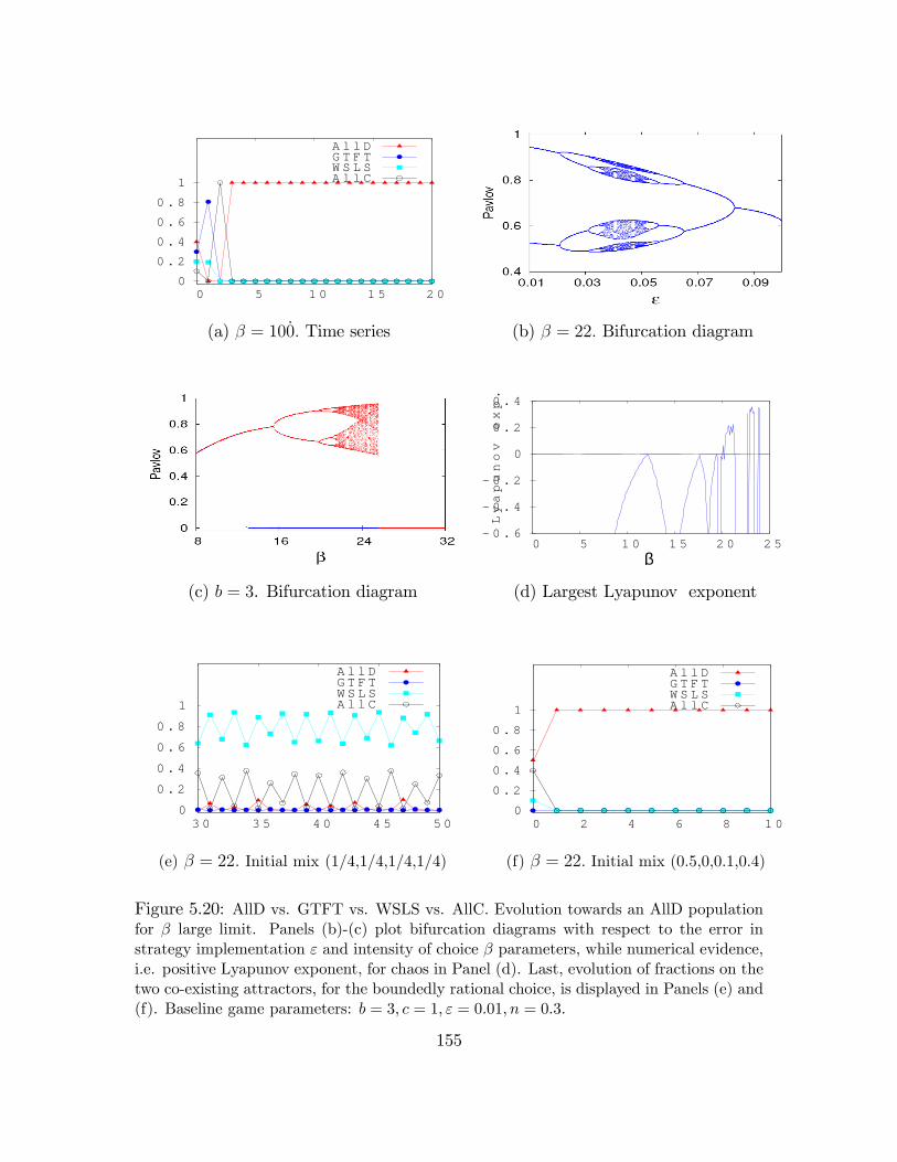
0

0 . 2

0 . 4

0 . 6

0 . 8

1

0 5 1 0 1 5 2 0

A l l DG T F TW S L SA l l C

(a) � = 10_0: Time series (b) � = 22: Bifurcation diagram

(c) b = 3. Bifurcation diagram

0 . 6

0 . 4

0 . 2

0

0 . 2

0 . 4

0 5 1 0 1 5 2 0 2 5

Lyapunov exp.

β

(d) Largest Lyapunov exponent

0

0 . 2

0 . 4

0 . 6

0 . 8

1

3 0 3 5 4 0 4 5 5 0


(e) � = 22: Initial mix (1/4,1/4,1/4,1/4)

0

0 . 2

0 . 4

0 . 6

0 . 8

1

0 2 4 6 8 1 0


(f) � = 22: Initial mix (0.5,0,0.1,0.4)

Figure 5.20: AllD vs. GTFT vs. WSLS vs. AllC. Evolution towards an AllD populationfor � large limit. Panels (b)-(c) plot bifurcation diagrams with respect to the error instrategy implementation " and intensity of choice � parameters, while numerical evidence,i.e. positive Lyapunov exponent, for chaos in Panel (d). Last, evolution of fractions on thetwo co-existing attractors, for the boundedly rational choice, is displayed in Panels (e) and(f). Baseline game parameters: b = 3; c = 1; " = 0:01; n = 0:3:

155

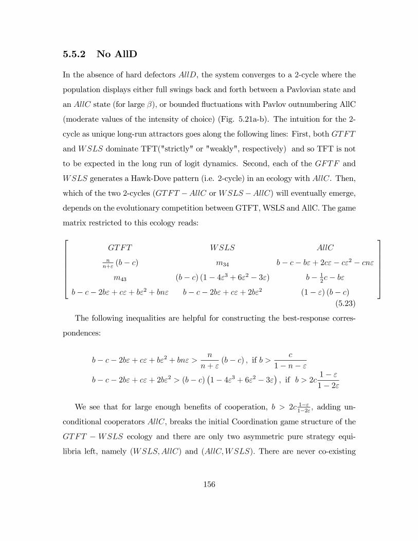
5.5.2 No AllD

In the absence of hard defectors AllD, the system converges to a 2-cycle where the

population displays either full swings back and forth between a Pavlovian state and

an AllC state (for large �); or bounded �uctuations with Pavlov outnumbering AllC

(moderate values of the intensity of choice) (Fig. 5.21a-b). The intuition for the 2-

cycle as unique long-run attractors goes along the following lines: First, both GTFT

and WSLS dominate TFT("strictly" or "weakly", respectively) and so TFT is not

to be expected in the long run of logit dynamics. Second, each of the GFTF and

WSLS generates a Hawk-Dove pattern (i.e. 2-cycle) in an ecology with AllC. Then,

which of the two 2-cycles (GTFT �AllC or WSLS �AllC) will eventually emerge,

depends on the evolutionary competition between GTFT, WSLS and AllC. The game

matrix restricted to this ecology reads:26666664GTFT WSLS AllC

nn+"

(b� c) m34 b� c� b"+ 2c"� c"2 � cn"

m43 (b� c) (1� 4"3 + 6"2 � 3") b� 12c� b"

b� c� 2b"+ c"+ b"2 + bn" b� c� 2b"+ c"+ 2b"2 (1� ") (b� c)

37777775(5.23)

The following inequalities are helpful for constructing the best-response corres-

pondences:

b� c� 2b"+ c"+ b"2 + bn" > n

n+ "(b� c) ; if b > c

1� n� "b� c� 2b"+ c"+ 2b"2 > (b� c)

�1� 4"3 + 6"2 � 3"

�; if b > 2c

1� "1� 2"

We see that for large enough bene�ts of cooperation, b > 2c 1�"1�2" ; adding un-

conditional cooperators AllC, breaks the initial Coordination game structure of the

GTFT � WSLS ecology and there are only two asymmetric pure strategy equi-

libria left, namely (WSLS;AllC) and (AllC;WSLS): There are never co-existing

156

two 2-cycles in this ecology. The WSLS � AllC 2-cycle depicted in Fig. 5.21a-

b for the "boundedly rational" and the "best-reply" repeated PD strategy choices,

respectively.

For c1�n�" < b < 2c

1�"1�2" we have AllC = BRfGTFTg, WSLS = BRfWSLSg,

WSLS = BRfAllCg and the population converges, for � ! 1; to a Pavlovian

WSLS monomorphism.

Last, for c < b < c1�n�" ; we have WSLS = BRfGTFTg so AllC is a strictly

dominated strategy. We are back in the GTFT � WSLS ecology where Pavlov

strictly dominates GTFT and, consequently, is the unique monomorphic long-run

outcome of Logit Dynamics (Panels (c), (d) for high and low values of � respectively).

We can conclude from this analysis that co-existence of two 2-cycles does not occur.

157

0

0 . 2

0 . 4

0 . 6

0 . 8

1

0 5 1 0 1 5 2 0

T F TG T F TW S L SA l l C

(a) b = 4; � = 15:Time series

0

0 . 2

0 . 4

0 . 6

0 . 8

1

0 2 4 6 8 1 0 1 2 1 4


(b) b = 4; � = 200:Time series

0

0 . 2

0 . 4

0 . 6

0 . 8

1

0 2 4 6 8 1 0 1 2 1 4


(c) b = 1:1; � = 600:Time series

0

0 . 2

0 . 4

0 . 6

0 . 8

1

0 2 4 6 8 1 0 1 2 1 4


(d) b = 1:1; � = 100:Time series

Figure 5.21: TFT vs. GTFT vs. WSLS vs. AllC. Panels (a)-(b): for large bene�ts ofcooperation, b = 4, fractions converge to a (WSLS, AllC) 2-cycle for both high and lowvalues of the intensity of choice. Panels (c)-(d): for low bene�t of cooperation, b = 1:1,system converges to a monomorphic Pavlovian state. Remaining game parameters: c =1; " = 0:01; n = 0:3:

158

5.5.3 No GTFT

Unlike the previous case, the 4�4 ecology withoutGTFT 21 exhibits path-dependence.

Hence, for moderate values of the intensity of choice � � 27, the system displays

co-existence of attractors. Depending on the initial population mix, the long-run

evolutionary outcome can be either the cyclical competition between AllD; TFT

and AllC with asymmetric amplitudes (time series Fig. 5.22b) as in subsection

(5.4.1), or a 1-piece chaotic attractor (time series in Fig. 5.22c) with Pavlov having

a dominant position, as in, for instance, subsection (5.4.6). In both cases, the other

strategies remain present in the population, but in small numbers.

For high values of � the path-dependence is lost, the only remaining attractor

being a full-ranged Rock-Paper-Scissors 3-cycle (Panel (d)) in AllD, TFT and AllC,

with stimulus-response players WSLS going extinct. The bifurcation diagram in

Panel (a) organizes the long-run outcomes of this ecology and displays the two co-

existing attractors: the chaotic one in the top and the cyclical one in the bottom

curves.

21Imhof et al. (2007) also discuss, in a �nite population framework, an ecology ofAllD; TFT;WSLS and AllC behaviors, under the frequency-dependent, mutation-selection Moranprocess. They show that AllD is selected for stage game payo¤s (i.e. b=c ratio) below a certainthreshold, while WSLS wins the evolutionary competition otherwise.

159

(a) b = 4:Bifurcation diagram showing

co-existence of attractors

0

0 . 2

0 . 4

0 . 6

0 . 8

1

2 0 2 5 3 0 3 5 4 0

A l l DT F T

W S L SA l l C

(b) small � = 27: Time series, initial

population mixture: (1/4,1/4,1/4,1/4)

0

0 . 2

0 . 4

0 . 6

0 . 8

1

2 0 3 0 4 0 5 0

A l l DT F T

W S L SA l l C

(c) small � = 27: Initial population

mixture: (10%,10%,50%,30%)

0

0 . 2

0 . 4

0 . 6

0 . 8

1

5 0 5 5 6 0 6 5 7 0

A l l DT F T

W S L SA l l C

(d) large � = 100: Initial population

mixture: (1/4,1/4,1/4,1/4)

Figure 5.22: AllD vs. TFT vs. WSLS vs. AllC. Panel (a) bifurcation diagram of Pavlovfractions with respect to the intensity of choice parameter; Panels (b)-(c): dependingon initial distribution of fractions the long-run population state may be either ongoingoscillations among AllD, TFT, AllC(Panel (b)) or co-existence, although in a possiblychaotic fashion, of WSLS and AllC players with WSLS largely outnumbering unconditionalcooperators (Panel (c)). Last, Panel (d) displays the large � limit of the long-run dynamicsof fractions. Remaining game parameters: b = 4; c = 1; " = 0:01; n = 0:3:

160

5.5.4 No WSLS

With the stimulus-response WSLS rule put aside, the evolutionary dynamics be-

comes very complicated. In the � large limit, co-existence of the four strategies in

a cyclical fashion, is observed for high bene�ts of cooperation b (Fig. 5.23a) while,

for low bene�ts b, GTFT is driven extinct and full-scale cyclical dynamics with the

remaining three strategies emerge (Panel (b)).

For �nite �; a stable limit cycle is born via a Neimark-Sacker bifurcation (Fig.

5.23a) for small b; while a period-doubling route to chaos emerges for high bene�ts

accrued to cooperation (Panel (d)). Finally, in Fig. 5.23e a period-doubling route to

chaos is depicted (positive Lyapunov exponent plot in Panel (f)) as the generosity

parameter n built into the GTFT strategy is �ne-tuned.

161

0

0 . 2

0 . 4

0 . 6

0 . 8

1

5 0 5 5 6 0 6 5 7 0

A l l DT F T

G T F TA l l C

(a) b = 2, large � = 100: Time series

0

0 . 2

0 . 4

0 . 6

0 . 8

1

5 0 5 5 6 0 6 5 7 0

A l l DT F T

G T F TA l l C

(b) b = 6, large � = 100: Time series

(c) b = 2. Bifurcation diagram � (d) b = 6. Bifurcation diagram �

(e) b = 6; � = 15: Bifurcation diagram n

0 . 8

0 . 6

0 . 4

0 . 2

0

0 . 2

0 . 2 0 . 2 5 0 . 3 0 . 3 5 0 . 4 0 . 4 5 0 . 5

Lyapunov exp.

n

(f) � = 15: Largest Lyapunov exponent

Figure 5.23: AllD vs. TFT vs. GTFT vs. AllC. Time series of the corresponding fractions,for large �, and large/small bene�t of cooperation (Panel (a) and (b), respectively) .Bifurcatins diagrams for high and low b are also shown in Panel (c)-(d). Last, Panel (e)displays a bifurcation diagram of GTFT fraction with respect to the "generosity" parametern while Panel (f) shows some numerical evidence for chaos. Remaining game parameters:c = 1; " = 0:01; n = 0:3:

162

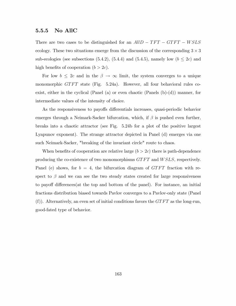
5.5.5 No AllC

There are two cases to be distinguished for an AllD � TFT � GTFT � WSLS

ecology. These two situations emerge from the discussion of the corresponding 3� 3

sub-ecologies (see subsections (5.4.2), (5.4.4) and (5.4.5), namely low (b � 2c) and

high bene�ts of cooperation (b > 2c).

For low b � 2c and in the � ! 1 limit, the system converges to a unique

monomorphic GTFT state (Fig. 5.24a). However, all four behavioral rules co-

exist, either in the cyclical (Panel (a) or even chaotic (Panels (b)-(d)) manner, for

intermediate values of the intensity of choice.

As the responsiveness to payo¤s di¤erentials increases, quasi-periodic behavior

emerges through a Neimark-Sacker bifurcation, which, if � is pushed even further,

breaks into a chaotic attractor (see Fig. 5.24b for a plot of the positive largest

Lyapunov exponent). The strange attractor depicted in Panel (d) emerges via one

such Neimark-Sacker, "breaking of the invariant circle" route to chaos.

When bene�ts of cooperation are relative large (b > 2c) there is path-dependence

producing the co-existence of two monomorphisms GTFT and WSLS, respectively.

Panel (e) shows, for b = 4, the bifurcation diagram of GTFT fraction with re-

spect to � and we can see the two steady states created for large responsiveness

to payo¤ di¤erences(at the top and bottom of the panel). For instance, an initial

fractions distribution biased towards Pavlov converges to a Pavlov-only state (Panel

(f)). Alternatively, an even set of initial conditions favors the GTFT as the long-run,

good-fated type of behavior.

163

(a) b = 2: Bifurcation (�;GTFT )

0 . 3

0 . 2

0 . 1

0

0 . 1

0 . 2

1 0 1 5 2 0 2 5 3 0 3 5

Lyapunov exp.

β

(b) b = 2: Lyapunov exponent

0

0 . 2

0 . 4

0 . 6

0 . 8

1

5 0 5 5 6 0 6 5 7 0

A l l DT F T

G T F TW S L S

(c) b = 2; � = 18: Time series (d) b = 2; � = 17:6. Strange attractor

(e) b = 4. Bifurcation diagram

0

0 . 2

0 . 4

0 . 6

0 . 8

1

0 5 1 0 1 5 2 0

A l l DT F T

G T F TW S L S

(f) � = 100: Initial mix: (0.1, 0.1, 0.1, 0.7)

Figure 5.24: AllD vs. TFT vs. GTFT vs. WSLS. Panels (a): bifurcation diagram withrespect to the intensity of choice showing quasi-periodic behavior. Panels (c)-(d): timeseries, phase portraint and Lyapunov exponent plot as numerical evidence for chaotic timeseries when the intensity of choice � increases. Finally, Panels (e)-(f) show the long-runbehavior, in the best-reply limit, for large bene�ts of cooperation: this is, co-existence ofmonomorphic GTFT and Pavlov WSLS states. Baseline game parameters: c = 1; " =0:01; n = 0:3:

164

5.5.6 Summary

Table 5.3 summarizes the long-run behavior of all 4 � 4 ecologies both the best-

reply (� large) and in the boundedly rational (� small) choice cases. In comparison

to the 3 � 3 ecologies reviewed in the previous section, having more strategies not

only enlarges the set of possible outcomes but also makes the behavior much more

complicated. In particular there is now strong path-dependence in most of the eco-

logies, leading to the co-existence of complicated attractors, periodic and chaotic

ones. We identi�ed two routes to complex dynamics in these 4 � 4 ecologies: the

period-doubling and breaking of the invariant circle route to chaos. However, the

path dependence is lost for some ecologies (subsections (5.5.1), (5.5.2), (5.5.3))) when

� approaches the "full rationality" limit. WSLS fares well in an AllD environment

with no AllC players, but poorly, almost going extinct, in an AllCenvironment with

AllD strategists around.

4x4 Bifurcations Attractors

small � large �

No AllD PD 2-cycle 2-cycle or unique SS

No TFT PD, NS co-existence SS and chaos unique SS (AllD)

No GTFT PD, NS co-existence RSP and chaos unique SS (AllD)

No WSLS NS limit cycles, chaos 4-cycle

No AllC NS, PD limit cycles, chaos multiple SS (GTFT, WSLS)

Table 5.3: Summary of the dynamical behaviour for all 4x4 interaction of iterated Pris-oner�s Dilemma strategies under logit dynamics.

165

5.6 5�5 Ecology

In this section, we report simulations about the behavior of Logit Dynamics on the

full 5� 5 ecology AllD � TFT �GTFT �WSLS �AllC that generated the game

matrix (5.3). Depending on the relative size of cooperation bene�ts we distinguish

again two situations.

First, for small bene�ts, b � 2c there is co-existence of all �ve strategies, albeit

in a �uctuating manner, for low responsiveness to payo¤s di¤erences (Fig. 5.25a).

When � reaches the best-response limit the long-run outcome is an AllD-TFT -AllC

3-cycle (Fig. 5.25b).

If the bene�ts of cooperation are large, Pavlov wins the evolutionary competition

for small � (Panel (c)) but goes extinct in the � ! 1 limit, with a 4-cycle in the

remaining strategies as long run behavior (Panel (d)). Last, Panels (e), (f) display

bifurcation diagrams of AllC and Pavlov fractions respectively with respect to the

intensity of choice. It is apparent from the AllC bifurcation diagram in Panel (e)

that an initially stable steady state for very low �; destabilizes for moderate values,

with continuous swings between high and low fractions emerging for large �: As

far as Pavlov is concerned the corresponding bifurcation diagram shows its way to

extinction when players choose a best-reply (Fig. 5.25f) .

The chaotic patterns in the two diagrams for intermediate values of � are con-

�rmed in Fig. 5.26a-f that displays two dimensional projections of a chaotic attractor

together with the fractions evolution on the attractor for b = 2:4805 and � = 15:

Finally, Fig. 5.27c-d illustrates the "breaking of an invariant circle" route to chaos:

a quasiperiodic attractor for � = 0:05 breaks into a 6-piece quasi-periodic and then

chaotic attractor (Panels (d)-(e)) at � � 10:05 and � = 10:2: Eventually these pieces

join together to form a 1-piece strange attractor (Fig. 5.27f) when the intensity of

choice � reaches the threshold � = 10:8:

166

0

0 . 2

0 . 4

0 . 6

0 . 8

1

5 0 5 2 5 4 5 6 5 8 6 0

A l l DT F T

G T F TW S L SA l l C


0 0 . 2 0 . 4 0 . 6 0 . 8

1

2 0 2 2 2 4 2 6 2 8 3 0

A l l DT F T


(b) b = 2; � = 300: Time series

0

0 . 2

0 . 4

0 . 6

0 . 8

1

5 0 5 2 5 4 5 6 5 8 6 0

A l l DT F T


(c) b = 4; � = 15: Time series

0 0 . 2 0 . 4 0 . 6 0 . 8

1

2 0 2 2 2 4 2 6 2 8 3 0

A l l DT F T


(d) b = 4; � = 150: Time series

(e) b = 4: Bifurcation diagram (f) b = 4: Bifurcation diagram

Figure 5.25: AllD vs. TFT vs. GTFT vs. WSLS vs. AllC. Panels (a)-(b) show the long-run outcome for low bene�ts of cooperation b in the � low and high limit, respectively.Similar time series are displayed in Panels (c)-(d) for the high bene�t b case. Panels (e)-(f) show, for high b, bifurcation diagrams of AllC and Pavlov fractions. Baseline gameparameters: c = 1; " = 0:01; n = 0:3:

167

(a) b = 2:48; � = 15: Strange attractor (b) b = 2:48; � = 15: Strange attractor

(c) b = 2:48; � = 15: Strange attractor (d) b = 2:48; � = 15: Strange attractor

0

0 . 2

0 . 4

0 . 6

0 . 8

1

4 0 4 5 5 0 5 5 6 0 6 5 7 0

A l l DT F T

G T F T

(e) b = 2:48; � = 15: Time series

0

0 . 2

0 . 4

0 . 6

0 . 8

1

4 0 4 5 5 0 5 5 6 0 6 5 7 0


(f) b = 2:48; � = 15: Time series

Figure 5.26: AllD vs. TFT vs. GTFT vs. WSLS vs. AllC. Panels (a)-(d): two-dimensionalprojections of a strange attractor for b = 2:4805 and � = 15. Panels (e)-(f) evolution offractions on the strange attractor. Remaining game parameters: c = 1; " = 0:01; n = 0:3:

168

(a) b = 2:48. Bifurcation diagram �

0 . 4

0 . 2

0

0 . 2

0 . 4

6 8 1 0 1 2 1 4

Lyapunov exp.

β

(b) b = 2:48:Lyapunov exponent

(c) � = 9:05: 1-piece attractor (d) � = 10:05: 6-piece quasiperiodic

(e) � = 10:2: 6-piece chaotic (e) � = 10:8: 1-piece chaotic

Figure 5.27: AllD vs. TFT vs. GTFT vs. WSLS vs. AllC. Panels (a)-(b): bifurcationdiagram with respect to intensity of choice � and numerical evidence of chaos (plot of thelargest Lyapunov exponent). Panels (c)-(f) show the evolution of a quasiperiodic attractorinto a strange attractor as the intensity of choice increases. Remaining game parameters:b = 2:48; c = 1; " = 0:01; n = 0:3:

169

5.6.1 Numerical Bifurcation Curves

The visual analysis of the bifurcation diagram in Fig. 5.25 can be con�rmed by a

rigorous continuation procedure, i.e. the computation of curves of equilibria along

with their detected codimension I bifurcations as one parameter is varied using the

Cl_Matcont bifurcation software package22 (Dhooge et al. (2003)). One such �xed

point - (0:4972065; 0:4178546; 0:06911757; 0:01521537; 0:01521537) for the game para-

meterization b = 1:1; c = 1; " = 0:01;n = 0:3; � = 14- is continued in Fig. 5.28 top

left panel, as the bene�t of cooperation b is increased. Three singularities are de-

tected by the continuation package in the meaningful region [b > c = 1] of b : two

Neimark-Sacker (NS) points at b = 1:270046 and b = 2:63647623 and one Period-

Doubling (PD) point at b = 3:158022: These two points are next �continued�with

respect to another parameter as depicted with codimension II singularities24 detec-

ted along them. The bifurcation curves describe in a systematic way the qualitative

changes in the behavior of the dynamical system in a certain parameters space. For

instance, in the two bottom panels in Fig. 5.28 the plotted curves of Neimark-Sacker

singularities partition the parameters space in regions with qualitatively similar be-

havior: when crossing a NS curve from below the system loses stability of the steady

state and a stable limit cycles arises around the unstable steady state. Such an ana-

lysis reveals that the behavior envisaged by simulations is robust to perturbations

of the repeated Prisoner�s Dilemma game (as parametrized by the b=c ratio), the

probability of mistake in implementing a particular strategy "; and the generosity

parameter n. Note that, compared to the 3 � 3 ecologies, there is no fold bifurc-

ation as coordination on equilibria is more di¢ cult to achieve with more strategies.

Instead, increasing the strategy space generates oscillatory behavior more easily.

22Cl_Matcont for maps, see package documentation at http://www.matcont.ugent.be/23normal form coe¢ cients are -2.741700 and -5.440686 meaning that the NS bifurcations are

supercritical, i.e. the limit cycles are born stable.24e.g. a Chenciner CH codim II bifurcation gives rise to much more complicated patterns

of behavior (see Kuznetsov (1995) pp. 482).

170

0 1 2 3 40

0 .3

0 .5

0 .7

0 .9PD

N S

N S

PD

b

% A

llD

5 10 15 20 25

0

2

4

6

8

10

CH

β

bene

fit o

f coo

pera

tion

b

PD

PD

NS

PDNS

PD

0.1 0 0.1 0.20

2

4

6

8

10

R1

R1

PDNSCH

CHPDNS

ε

bene

fit o

f coo

pera

tion

b

PD

PDPD

PDNS

NS

0 0.2 0.4 0.6 0.8 10

1

2

3

4

GPD

CHR1

PDNS

PDNS

n

bene

fit o

f coo

pera

tion

b

NS

NS NS

NS

PD PD

PDPD

0 0.2 0.4 0.6 0.85

10

15

20

25

R1

CHR1

n

β

NS

NSNS

NS

stablesteady state

stablelimit cycle

stablelimit cycle

stablelimit cycle

0.05 0 0.05 0.15

10

15

20

25

CH

R1

ε

β

NS NS

stablelimit cycle

stablelimit cycle

stablesteady state

NSNS

Figure 5.28: AllD vs. TFT vs. GTFT vs. WSLS vs. AllC. Top left Panel continues a nu-merically computed �xed point, in the bene�t of cooperation space. Detected codimensionI singularities are then continued with respect to another game/behavioral parameter. Theresulting curves of Period-Doubling (PD) and Neimark-Sacker (NS) points, with respectto the intensity of choice �, probability of error in strategy execution ", and degree ofgenerosity n, are plotted in the top-right, middle and bottom panels, respectively. Theoccurrence of codimension II singularities can be observed along all these curves. Unlessfree to �oat, game parameters set to: b = 2; c = 1; " = 0:01; n = 0:3; � = 15

171

5.7 Conclusions

In an evolutionary set-up, we append an ecology of iterated Prisoner�s Dilemma

(IPD) game strategies, consisting of unconditional cooperators (AllC), uncondi-

tional defectors (AllD) and reactive players (TFT ) with two repeated strategies that

have received less attention in the evolutionary IPD game literature, the error-proof,

"generous" tit-for-tat (GTFT ) which, with a certain probability, re-establishes co-

operation after a (possibly by mistake) defection of the opponent and the penitent,

"stimulus-response" (WSLS) strategy that resets cooperation after the opponent

punished for defection. Stable oscillations in the frequency of both the forgiving

(GTFT ) and repentant (Pavlov) strategy along with chaotic behavior emerge under

a perturbed version of best-response dynamics, the logit dynamics. We have per-

formed a detailed analysis of the relatively simple 2 � 2 and 3 � 3 case with the

dynamic behaviour now fairly well understood. However, the enlarged 4 � 4 and

5� 5 exhibit complicated behavior via period-doubling and breaking of an invariant

circle routes to chaos. Finite intensity of choice � leads to rich dynamics, path-

dependence and co-existence of cyclical and chaotic attractors for a wide selection

of 4 � 4 ecologies. If we turn to the best-reply limit of the logit dynamics, various

3�and 4�cycles are exhibited in speci�c 4 � 4 and in the 5 � 5 ecologies. Last, in

terms of individual strategies performance, we discovered �rst that the presence of

unconditional cooperators turns out detrimental to the discriminating types (TFT ,

GTFT and WSLS) in some 4x4 interactions leading the population to an AllD

monomorphism. Second, there is mixed evidence for a Pavlovian meta-rule in an

evolutionary repeated PD with a population of rational players: on the one hand,

the stimulus-response strategy does very well and wins the evolutionary competi-

tion in a 4 � 4 environment with hard defectors (AllD) but no undiscriminating

cooperators(AllC), but it almost goes extinct in the full 5�5 repeated game. Never-

theless, with boundedly rational players, the fractions of Pavlov maintain high values

even within the complete ecology of �ve rules.

172

5.A Iterated PDGame-stationary distributions and

average payo¤s

For each pairwise interaction of the iterated PD strategies Si � Sj, the stationary

distribution = f�CC ; �CD; �DC ; �DDg gives the average fraction of time system

spends in each of the four states CC;CD;DC;DD, respectively. Average expected

payo¤s are computed as weighted average of the stage game matrix payo¤s with

weights obtained from the stationary distribution:

�i(Si;Sj) =

26666664b� c

�c

b

0

37777775

T 26666664�CC

�CD

�DC

�DD

37777775i; j 2 fAllD; TFT;GTFT;WSLS;AllCg

Using the transition probability matrix (5.2) we can derive the stationary distri-

bution together with the respective average expected payo¤s as summarized in the

following table (some expression mij are too long and given at the end of the table):

173

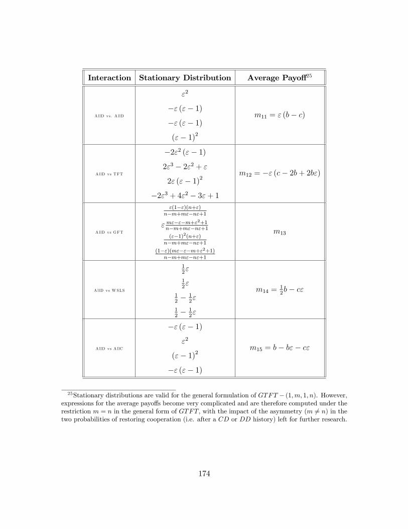
Interaction Stationary Distribution Average Payo¤25

AllD vs. A llD

"2

�" ("� 1)

�" ("� 1)

("� 1)2

m11 = " (b� c)

AllD vs TFT

�2"2 ("� 1)

2"3 � 2"2 + "

2" ("� 1)2

�2"3 + 4"2 � 3"+ 1

m12 = �" (c� 2b+ 2b")

AllD vs GFT

"(1�")(n+")n�m+m"�n"+1

" m"�"�m+"2+1

n�m+m"�n"+1("�1)2(n+")

n�m+m"�n"+1(1�")(m"�"�m+"2+1)

n�m+m"�n"+1

m13

AllD vs WSLS

12"

12"

12� 1

2"

12� 1

2"

m14 =12b� c"

AllD vs A llC

�" ("� 1)

"2

("� 1)2

�" ("� 1)

m15 = b� b"� c"

25Stationary distributions are valid for the general formulation of GTFT � (1;m; 1; n). However,expressions for the average payo¤s become very complicated and are therefore computed under therestriction m = n in the general form of GTFT; with the impact of the asymmetry (m 6= n) in thetwo probabilities of restoring cooperation (i.e. after a CD or DD history) left for further research.

174

Interaction Stationary Distribution Payo¤s

TFT vs A llD

�2"2 ("� 1)

2" ("� 1)2

2"3 � 2"2 + "

�2"3 + 4"2 � 3"+ 1

m21

TFT vs TFT

1=4

1=4

1=4

1=4

m22 =12b� 1

2c

TFT vs. GTFT

(1�")(n+")(m+"�2m")m"+5n"+9"2�12"3+4"4�6m"2+4m"3�10n"2+4n"3+mn�4mn"+4mn"2

2"2 "�12"�2"2 (m+"�2)("+n�2n")

m"+5n"+9"2�12"3+4"4�6m"2+4m"3�10n"2+4n"3+mn�4mn"+4mn"2

2"("�1)2(n+")m"+5n"+9"2�12"3+4"4�6m"2+4m"3�10n"2+4n"3+mn�4mn"+4mn"2

2"2("�1)(m+"�2)m"+5n"+9"2�12"3+4"4�6m"2+4m"3�10n"2+4n"3+mn�4mn"+4mn"2

m23

TFT vs. W SLS

1=4

1=4

1=4

1=4

m24 =12b� 1

2c

TFT vs A llC

� ("� 1) (2"2 � 2"+ 1)

�2"2 "�12"�2"2 (2"

2 � 2"+ 1)

2" ("� 1)2

�2"2 ("� 1)

m25

175


GTFT vs. A llD

�" ("� 1) n+"n�m+m"�n"+1

("� 1)2 n+"n�m+m"�n"+1

" m"�"�m+"2+1

n�m+m"�n"+1

� ("� 1) m"�"�m+"2+1n�m+m"�n"+1

m31

GTFT vs. TFT

(1�")(n+")(m+"�2m")m"+5n"+9"2�12"3+4"4�6m"2+4m"3�10n"2+4n"3+mn�4mn"+4mn"2

2"("�1)2(n+")m"+5n"+9"2�12"3+4"4�6m"2+4m"3�10n"2+4n"3+mn�4mn"+4mn"2

2"2 "�12"�2"2 (m+"�2)("+n�2n")

m"+5n"+9"2�12"3+4"4�6m"2+4m"3�10n"2+4n"3+mn�4mn"+4mn"2

2"2("�1)(m+"�2)m"+5n"+9"2�12"3+4"4�6m"2+4m"3�10n"2+4n"3+mn�4mn"+4mn"2

m32

GTFT vs. GTFT

�n 2m�2m"+n"�mn"3�2"2�4n"+mn2+m"2+2n"2+n2"�2mn+2mn"

n" n+"�2"3�2"2�4n"+mn2+m"2+2n"2+n2"�2mn+2mn"

n" n+"�2"3�2"2�4n"+mn2+m"2+2n"2+n2"�2mn+2mn"

"2 m+"�2"3�2"2�4n"+mn2+m"2+2n"2+n2"�2mn+2mn"

m33

GTFT vs. W SLS

(n+"�2n"�"2+2n"2�mn+2mn")("�1)4m"�7"�n+4n"+15"2�12"3+4"4�8m"2+4m"3�8n"2+4n"3+mn�4mn"+4mn"2

(n"�2"+"2+1)2"("�1)4m"�7"�n+4n"+15"2�12"3+4"4�8m"2+4m"3�8n"2+4n"3+mn�4mn"+4mn"2

�(2"�2m"�n"�3"2+"3+4m"2�2m"3+2n"2+mn"�2mn"2)4m"�7"�n+4n"+15"2�12"3+4"4�8m"2+4m"3�8n"2+4n"3+mn�4mn"+4mn"2

(m"�"�m+"2+1)2"("�1)4m"�7"�n+4n"+15"2�12"3+4"4�8m"2+4m"3�8n"2+4n"3+mn�4mn"+4mn"2

m34

GTFT vs. A llC

� "�1n"�m"+1 (n"� 2"+ "

2 + 1)

"n"�m"+1 (n"� 2"+ "

2 + 1)

" ("� 1) m+"�2n"�m"+1

�"2 m+"�2n"�m"+1

m35

176


WSLS vs. A llD

12"

12�12"

12"

12�12"

m41 = b"�12c

WSLS vs. TFT

1=4

1=4

1=4

1=4

m42 =12(b� c)

WSLS vs. GTFT

(n+"�2n"�"2+2n"2�mn+2mn")("�1)4m"�7"�n+4n"+15"2�12"3+4"4�8m"2+4m"3�8n"2+4n"3+mn�4mn"+4mn"2

�(2"�2m"�n"�3"2+"3+4m"2�2m"3+2n"2+mn"�2mn"2)4m"�7"�n+4n"+15"2�12"3+4"4�8m"2+4m"3�8n"2+4n"3+mn�4mn"+4mn"2

(n"�2"+"2+1)2"("�1)4m"�7"�n+4n"+15"2�12"3+4"4�8m"2+4m"3�8n"2+4n"3+mn�4mn"+4mn"2

(m"�"�m+"2+1)2"("�1)4m"�7"�n+4n"+15"2�12"3+4"4�8m"2+4m"3�8n"2+4n"3+mn�4mn"+4mn"2

m43

WSLS vs. W SLS

�4"3+7"2�4"+ 1

�" ("� 1)

�" ("� 1)

4"3�5"2+2"

m44

WSLS vs. A llC

12�12"

12"

12�12"

12"

m45

177


AllC vs. A llD

�" ("� 1)

("� 1)2

"2

�" ("� 1)

m51 = b"� c+ c"

AllC vs. TFT

�2"3 + 4"2 � 3"+ 1

2" ("� 1)2

2"3 � 2"2 + "

�2"2 ("� 1)

m52 = b� c� 2b"+ c"+ 2b"2

AllC vs. GTFT

� "�1n"�m"+1 (n"� 2"+ "

2 + 1)

" ("� 1) m+"�2n"�m"+1

"n"�m"+1 (n"� 2"+ "

2 + 1)

�"2 m+"�2n"�m"+1

m53 = b� c� 2b"+ c"+ b"2 + bn"

AllC vs. W SLS

�2"3 + 4"2 � 3"+ 1

2" ("� 1)2

2"3 � 2"2 + "

�2"2 ("� 1)

m54 = b� c� 2b"+ c"+ 2b"2

AllC vs. A llC

("� 1)2

�" ("� 1)

�" ("� 1)

"2

m55 = (1� ") (b� c)

Table 5.4: Stationary distributions and average expected payo¤s for an iterated PD gamewith an ecology of repeated rules consisting of AllD, TFT, GTFT, WSLS and AllC

178

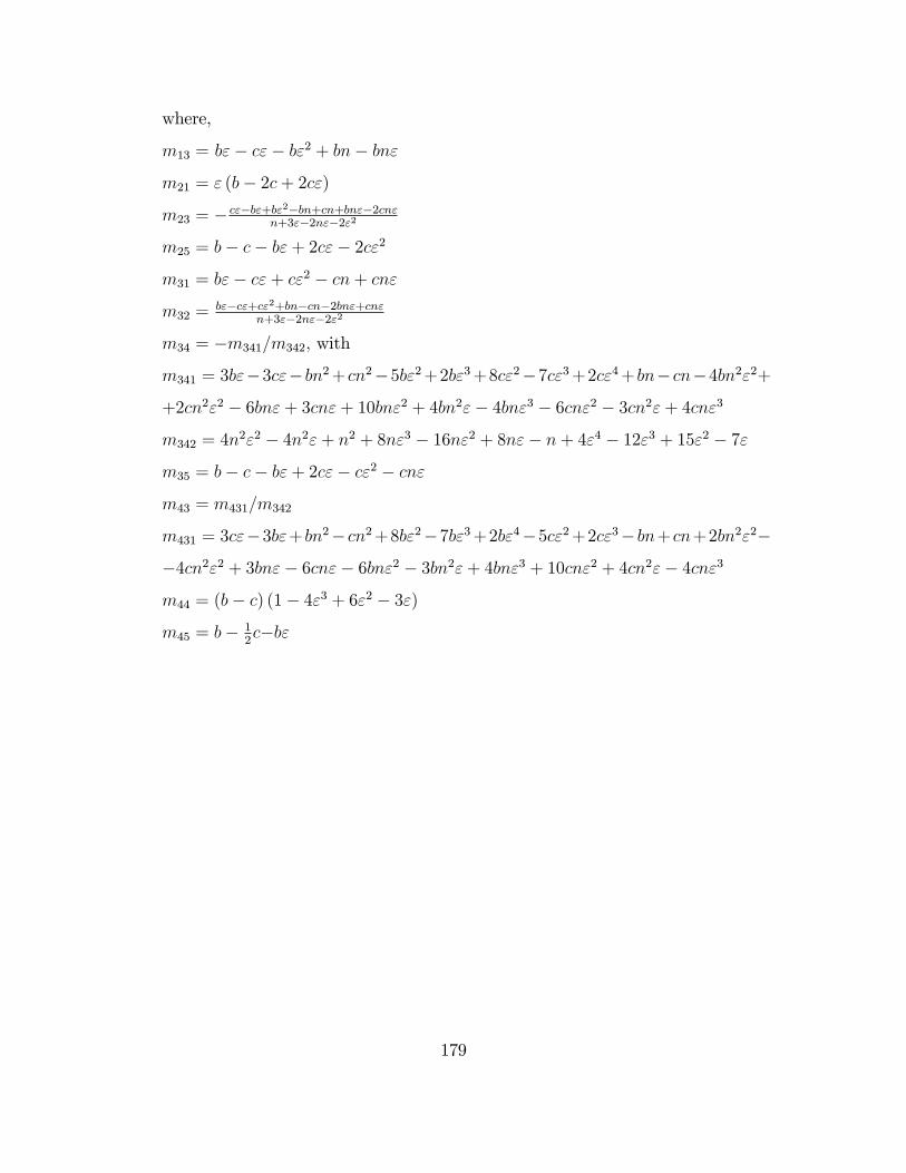
where,

m13 = b"� c"� b"2 + bn� bn"

m21 = " (b� 2c+ 2c")

m23 = � c"�b"+b"2�bn+cn+bn"�2cn"n+3"�2n"�2"2

m25 = b� c� b"+ 2c"� 2c"2

m31 = b"� c"+ c"2 � cn+ cn"

m32 =b"�c"+c"2+bn�cn�2bn"+cn"

n+3"�2n"�2"2

m34 = �m341=m342; with

m341 = 3b"�3c"� bn2+cn2�5b"2+2b"3+8c"2�7c"3+2c"4+ bn�cn�4bn2"2+

+2cn2"2 � 6bn"+ 3cn"+ 10bn"2 + 4bn2"� 4bn"3 � 6cn"2 � 3cn2"+ 4cn"3

m342 = 4n2"2 � 4n2"+ n2 + 8n"3 � 16n"2 + 8n"� n+ 4"4 � 12"3 + 15"2 � 7"

m35 = b� c� b"+ 2c"� c"2 � cn"

m43 = m431=m342

m431 = 3c"�3b"+ bn2�cn2+8b"2�7b"3+2b"4�5c"2+2c"3� bn+cn+2bn2"2�

�4cn2"2 + 3bn"� 6cn"� 6bn"2 � 3bn2"+ 4bn"3 + 10cn"2 + 4cn2"� 4cn"3

m44 = (b� c) (1� 4"3 + 6"2 � 3")

m45 = b� 12c�b"

179

Chapter 6

Summary

The aim of this thesis is to study the dynamics of evolutionary games. Initially, evol-

utionary game theory has been viewed as an evolutionary "repair" of rational actor

game theory in the hope that a population of boundedly rational players may attain

convergence to classic "rational" solutions such as the Nash Equilibrium through

some learning or evolutionary process occuring at the population level. However,

there is still no class of evolutionary dynamics, neither simple, imitative learning

(Replicator Dynamics) nor involved, belief-based learning (Fictitious Play or Best

Reply Dynamics), guaranteeing convergence to Nash equilibrium, beyond certain

restricted classes of games, usually with a small number of strategies.

In this thesis the model of boundedly rational players is a perturbed version

of the best-reply choice, the so-called Logit rule. The strategic context to which

this evolutionary process is applied varies from simple models of cyclical competi-

tion ( Rock-Paper-Scissors), through industrial organization (Cournot game) and to

collective-action choice (repeated Prisoner�s Dilemma) games. The logit choice rule

has the appealing property of capturing a continuum of degrees of (myopic) rational

behavior through di¤erential responsiveness to payo¤di¤erences between alternative

choices. The connecting line through the chapters lies in the question whether a

steady state is obtained as long run outcome of the Logit evolutionary dynamics or

181

whether multiple steady states (path-dependence) or more complicated, cyclical or

perhaps chaotic attractors, may emerge as well.

Chapter 2 contrasts the long-run behavior of Replicator and Logit Dynamics in

standard Rock-Paper-Scissors and Coordination games. It is well known that Rep-

licator Dynamics does not give rise to a stable limit cycle but to heteroclinic cycles

in 3 � 3 circulant RSP games (Zeeman (1980)). We obtain an alternative proof

of this classical result based on the computation of the �rst Lyapunov coe¢ cient in

the normal form of the vector �eld induced by the Replicator Dynamics, and show

that all Hopf bifurcations are degenerate. Via the same technique, generic Hopf bi-

furcations are shown to occur under the Logit Dynamics and, moreover, all these

bifurcations are supercritical, i.e. the system exhibits stable limit cycles. This result

is extended, through continuation analysis with the Matcont software package to

the class of 3 � 3 non-circulant RSP games. Besides generic Hopf bifurcation, fold

singularities (i.e. creation of multiple interior steady states) also do not occur in

3� 3 games under Replicator Dynamics (Zeeman (1980)). With the help of a simple

3�3 Coordination game we detect numerically a scenario with three consecutive fold

bifurcations under the Logit Dynamics giving rise to multiple interior steady states.

Both the Hopf and fold codimension I singularites are continued in the game payo¤s

parameters and a behavioral parameter such as the intensity of choice, in order to

obtain bifurcation curves in the parameter space along with certain codimension II

singularities along these curves. A frequency-weighted version of the Logit dynamics

(iLogit) is put at work on the circulant 3 � 3 RSP game and shown to generate

stable limit cycles with a large amplitude reminiscent of the heteroclinic cycle con-

necting the three monomorphic steady states in the Replicator Dynamics. Unlike

Logit Dynamics, iLogit runs into chaotic behavior in an example of 4x4 symmetric,

biologically-inspired game.

While Chapter 2 focuses on the actions chosen in a particular strategic situation,

Chapter 3 investigates a deeper level of evolution of learning rules, in the context of a

182

linear inverse demand-quadratic costs Cournot duopoly. Besides choosing an action

in the stage quantity-setting game as a response to expectations about the choice

of the opponent (i.e. her quantity produced), players also have to make a decision

about the learning heuristic employed to form their expectations. This higher-order

competition between the expectation-formation rules has an impact on the stability

property of the underlying stage game Cournot-Nash equilibrium. Various pairs of

ecologies are drawn from a toolbox consisting of naive, adaptive, (weighted) �ctitious

play or rational (Nash) strategy. For instance, the evolutionary competition between

a free adaptive and a costly weighted �ctitious play rule destabilizes the Cournot-

Nash equilibrium through a primary period-doubling bifurcation and a secondary

Neimark-Sacker bifurcation and eventually enters a chaotic regime. This analysis

is extended in Chapter 4 to linear inverse demand linear costs Cournot games with

an arbitrary number of players in the spirit of the Theocharis (1960) "two is stable,

three is unstable" result. In a heterogenous learning rules environment consisting of

adaptive and rational players we show that the Cournot-Nash equilibrium destabil-

izes through a period-doubling route to chaos as the number of players increases.

Theocharis (1960) unstable triopoly is derived as the limit of a system with ho-

mogenous (no switching) naive expectation. Interestingly, it could be stabilized by

adjusting the model parameters, for instance, by making the expectations more ad-

aptive (placing higher weights on remote past observations).

Bounded rationality models with heterogenous players endowed with smart and

simple heuristics (Gigerenzer and Todd (1999)) emerges as a promising way out of

the conundrum of observed cooperation in collective action dilemmas. An ecology of

simple rules in an iterated Prisoner�s Dilemma framework is constructed in Chapter

5 with the selection of rules driven by a logistic-type of evolutionary dynamics. It

consists of reciprocators, unconditional defectors and cooperators, stimulus-response

(Pavlov) and generous reciprocators all subject to small implementation errors in

strategy execution and small mistakes in selecting the best-performing heuristic

183

available in the population. The evolutionary selection dynamics in the resulting

subecologies of rules are investigated by a mixture of analytical and numerical meth-

ods, with rich dynamical behaviour unfolding. The surrounding ecology appears

critical for the success or failure of certain heuristics and there is no "undisputed"

winner. Pavlov (stimulus-response) players do well in an environment without un-

conditional cooperators, but poorly when such indiscriminatingly "nice" players are

around. Rock-Paper-Scissors cycles arise in the 3 � 3 ecologies while some 4 � 4

ecologies easily display path-dependence and co-existence of periodic and chaotic

attractors.

A general conclusion of this thesis is that the evolutionary selection among

boundedly rational strategies does not necessarily ensure convergence to Nash equi-

librium and a richer dynamical behavior may be the rule rather than the exception.

184

Bibliography

Aguiar, M. and S. Castro (2008). Chaotic and deterministic switching in a two-person

game. Univ. of Porto Working Paper .

Akin, E. (1982). Cycling in simple genetic systems. Journal of Mathematical Bio-

logy 13, 305�324.

Alos-Ferrer, C. (2004). Cournot versus walras in dynamic oligopolies with memory.

International Journal of Industrial Organization 22, 193�217.

Anderson, S., A. de Palma, and J. Thisse (1992). Discrete Choice Theory of Product

Di¤erentiation. Cambrige, MA: MIT Press.

Axelrod, R. (1997). The Complexity of Cooperation: Agent-Based Models of Com-

petition and Collaboration. Princeton University Press.

Berger, U. (2005). Fictitious play in 2xn games. Journal of Economic Theory 120,

139½U154.

Berger, U. (2007). Two more classes of games with the continuous-time �ctitious

play property. Games and Economic Behavior 60(2), 247�261.

Berger, U. (2008). Learning in games with strategic complementarities revisited.

Journal of Economic Theory 143(1), 292�301.

Berger, U. and J. Hofbauer (2006). Irrational behavior in brown-von neumann-nash

dynamics. Games and Economic Behavior 56, 1�6.

185

Binmore, K. (1987). Modeling rational players, part i. Economics and Philosophy 3,

179�214.

Bomze, I. M. (1983). Lotka-volterra equation and replicator dynamics: two-

dimensional classi�cation. Biological Cybernetics 48, 201�211.

Bomze, I. M. (1995). Lotka-volterra equation and replicator dynamics: new issues

in classi�cation. Biological Cybernetics 72, 447�453.

Brock, W. and C. H. Hommes (1997). A rational route to randomness. Economet-

rica 65, 1059�1095.

Brown, G. W. (1951). Iterative solution of games by �ctitious play. In T. Koopmans

(Ed.), Activity Analysis of Production and Allocation, pp. 374�376. Wiley, New

York.

Camerer, C. F. (2003). Behavioral Game Theory: Experiments in Strategic Interac-

tion. Princeton University Press.

Chawanya, T. (1997). Coexistence of in�nitely many attractors in a simple �ow.

Physica D 109(3-4), 201�241.

Cheung, Y.-W. and D. Friedman (1997). Individual learning in normal form

games:some laboratory results. Games and Economic Behavior 19, 46�76.

Cournot, A. (1838). Researches into the Mathematical Principles of the Theory of

Wealth. Published in 1960, A. M. Kelley, New York.

Cox, J. C. and M. Walker (1998). Learning to play cournot duopoly strategies.

Journal of Economic Behavior and Organization 36, 141�161.

Cressman, R. (1997). Local stability of smooth selection dynamics for normal form

games. Mathematical Social Sciences 34, 1�19.

186

Deschamp, R. (1975). An algorithm of game theory applied to the duopoly problem.

European Economic Review 6, 187�194.

Dhooge, A., W. Govaerts, and Y. A. Kuznetsov (2003). Matcont: A matlab package

for numerical bifurcation analysis of odes. ACM Transactions on Mathematical

Software 29(2), 141 �164.

Dhooge, A., W. Govaerts, Y. A. Kuznetsov, W. Mestrom, and A. M. Riet (2003).

Clmatcont: a continuation toolbox in matlab. Symposium on Applied Comput-

ing, Proceedings of the 2003 ACM symposium on Applied computing, Melbourne,

Florida, 161 �166.

Droste, E., C. Hommes, and J. Tuinstra (2002). Endogenous �uctuations under

evolutionary pressure in cournot competition. Games and Economic Behavior 40,

232�269.

Fisher, F. (1961). The stability of the cournot solution: The e¤ects of speeds of

adjustment and increasing marginal costs. Review of Economic Studies 28 (2),

125�135.

Foster, D. and H. Young (1998). On the nonconvergence of �ctitious play in coordin-

ation games. Games and Economic Behavior 25, 79�96.

Fudenberg, D. and D. K. Levine (1998). The Theory of Learning in Games. MIT.

Gigerenzer, G. and P. M. Todd (1999). Simple Heuristics That Make Us Smart.

Cambridge University Press.

Gilboa, I. and A. Matsui (1991). Social stability and equilibrium. Econometrica 59,

859½U867.

Hahn, F. H. (1962). The stability of the cournot oligopoly solution. Review of

Economic Studies 27, 133�134.

187

Hahn, S. (1999). The convergence of �ctitious play in 3x3 games with strategic

complementarities. Economics Letters 64, 57�60.

Hofbauer, J. (1981). On the occurrence of limit cycles in the lotka-volterra di¤erential

equation. Journal of Nonlinear Analysis 5, 1003�1007.

Hofbauer, J. (2000). From nash and brown to maynard smith: equilibria, dynamics

and ess. Selection 1, 81�88.

Hofbauer, J. and W. Sandholm (2002). On the global convergence of stochastic

�ctitious play. Econometrica 70 (6), 2265�2294.

Hofbauer, J., P. Schuster, K. Sigmund, and R. Wol¤ (1980). Dynamical systems

under constant organization ii: homogeneous growth functions of degree p=2.

SIAM Journal on Applied Mathematics 38 (2), 282�304.

Hofbauer, J. and K. Sigmund (2003). Evolutionary Games and Population Dynamics.

Cambridge, UK: Cambridge University Press.

Hofbauer, J. and J. Weibull (1996). Evolutionary selection against dominated

strategies. Journal of Economic Theory 71, 558�573.

Hommes, C. H., H. Huang, and D. Wang (2005). A robust rational route to ran-

domness in a simple asset pricing model. Journal of Economic Dynamics and

Control 29, 1043�1072.

Huck, S., H. T. Normann, and J. Oechssler (2002). Stability of the cournot process-

experimental evidence. International Journal of Game Theory 31, 123�136.

Imhof, L., D. Fudenberg, and M. A. Nowak (2007). Tit-for-tat or win-stay, lose-shift?

Journal of Theoretical Biology 247(3), 574�580.

Jordan, S. (1993). Three problems in learning mixed-strategy nash equilibria. Games

and Economic Behavior 5, 368�386.

188

Juang, W. T. (2002). Rule evolution and equilibrium selection. Games and Economic

Behavior 39(1), 71�90.

Kandori, M., G. Mailath, and R. Rob (1993). Learning, mutation, and long run

equilibria in games. Econometrica 61, 29�56.

Kaniovski, Y., A. V. Kryazhimskii, and H. P. Young (2000). Adaptive dynamics in

games played by heterogeneous populations. Games and Economic Behavior 31(1),

50�96.

Kemeny, J. G. and J. L. Snell (1975). Denumerable Markov chains. New-York:

Springer-Verlag.

Kopel, M. (1996). Simple and complex ajustment dynamics in cournot duopoly

models. Chaos, Solitons & Fractals 7 (12), 2031�2048.

Kraines, D. and V. Kraines (1995). Evolution of learning among pavlov strategies.

Journal of Con�ict Resolution 39, 439�466.

Kraines, D. and V. Kraines (2000). Natural selection of memory-one strategies for

the iterated prisoner�s dilemma. Journal of Theoretical Biology 203, 335�355.

Krishna, V. (1992). Learning in games with strategic complementarities. HBS Work-

ing Paper 92-073, Harvard University 1992.

Krishna, V. and T. Sjöström (1998). On the convergence of �ctitious play. Mathem-

atics of Operations Research 23, 479�511.

Kuznetsov, Y. A. (1995). Elements of applied bifurcation theory. Berlin and New-

York: Springer-Verlag.

Maynard Smith, J. and J. Hofbauer (1987). The �battle of sexes�: a genetic model

with limit cycle behavior. Theoretical Population Biology 32, 1�14.

189

McFadden, D. (1981). Structural discrete probability models derived from theories of

choice. In C. Manski and D. L. McFadden (Eds.), Structural Analysis of Discrete

Data and Econometric Applications. Cambridge, MA: MIT Press.

McManus, M. (1964). Equilibrium, numbers and size in cournot oligopoly. Yorkshire

Bulletin of Social Science and Economic Research 16, 68�75.

Milgrom, P. and J. Roberts (1991). Adaptive and sophisticated learning in normal

form games. Games and Economic Behavior 3, 82�100.

Miyasawa, K. (1961). On the convergence of the learning process in a 2x2 non

zero-sum two person game. Research Memorandum, Economic Research Program,

Princeton University 33.

Monderer, D. and A. Sela (1996). A 2x2 game without the �ctitious play property.

Games and Economic Behavior 14, 144�148.

Monderer, D. and L. Shapley (1996a). Potential games. Games and Economic

Behavior 14, 124�143.

Monderer, D. and L. S. Shapley (1996b). Fictitious play property for games with

identical interests. Journal of Economic Theory 68(1), 258�265.

Nachbar, J. H. (1990). Evolutionary selection dynamics in games: convergence and

limit properties. International Journal of Game Theory 19, 59�89.

Okuguchi, K. (1970). Adaptive expectations in an oligopoly model. The Review of

Economics Studies 37 (2), 233�237.

Osborne, M. J. and A. Rubinstein (1994). A course in game theory. MIT Press.

Rand, D. (1978). Exotic phenomena in games and duopoly models. Journal of

Mathematical Economics 5, 173�184.

190

Richards, D. (1997). The geometry of inductive reasoning in games. Economic

Theory 10, 185�193.

Robinson, J. (1951). An iterative method of solving a game. Annals of Mathemat-

ics 54, 296�301.

Samuelson, L. and J. Zhang (1992). Evolutionary stability in asymmetric games.

Journal of Economic Theory 57, 363�391.

Sandholm, W. (2005). Excess payo¤ dynamics and other well-behaved evolutionary

dynamics. Journal of Economic Theory 124, 149�170.

Sandholm, W. (2008). Deterministic evolutionary dynamics. In S. N. Durlauf and

L. E. Blume (Eds.), New Palgrave Dictionary of Economics (2nd ed.). Palgrave

Macmillan, New York.

Sato, Y., E. Akiyama, and J. D. Farmer (2002). Chaos in learning a simple two-

person game. Proc. Natl. Acad. Sci. USA 99, 4748�4751.

Schuster, P., W. Schnabl, P. F. Stadler, and C. Forst (1991). Full characterization

of a strange attractor: chaotic dynamics in low-dimensional replicator systems.

Physica D 48, 65�90.

Shapley, L. (1964). Some topics in two-person games. In M. Drescher, L. Shapley,

and A. Tucker (Eds.), Advances in Game Theory. Princeton: Princeton University

Press.

Sigmund, K. and H. Brandt (2006). The good, the bad and the discriminator - errors

in direct and indirect reciprocity. Journal of Theoretical Biology 239, 183�194.

Sigmund, K. and M. A. Nowak (1993a). Chaos and the evolution of cooperation.

PNAS 90(11), 5091�5094.

191

Sigmund, K. and M. A. Nowak (1993b). Win-stay, lose-shift outperforms tit-for-tat.

Nature 364, 56�58.

Skyrms, B. (1992). Chaos in game dynamics. Journal of Logic, Language and In-

formation 1, 111�130.

Skyrms, B. (2000). Stability and explanatory signi�cance of some simple evolutionary

models. Philosophy of Science 67, 94�113.

Sparrow, C. and S. van Strien (2009). Fictitious play in 3x3 games: chaos and

dithering behaviour. Preprint March 2009 . Preprint March 2009.

Sparrow, C., S. van Strien, and C. Harris (2008). Fictitious play in 3x3 games:

The transition between periodic and chaotic behaviour. Games and Economic

Behavior 63(1), 259�291.

Stadler, P. and P. Schuster (1990). Dynamics of small autocatalytic reaction

networks-i bifurcations, permanence and exclusion. Bulletin of Mathematical Bio-

logy 52(4), 485�508.

Szidarovszky, F., S. Rassenti, S. S. Reynolds, and V. Smith (2000). Adaptation

and convergence of behaviour in repeated experimental cournot games. Journal of

Economic Behavior and Organization 41, 117�146.

Szidarovszky, F., S. Rassenti, and J. Yen (1994). The stability of the cournot solution

under adaptive expectations: a further generalization. International Review of

Economics and Finance 3 (2), 173�181.

Taylor, P. and L. Jonker (1978). Evolutionarily stable strategies and game dynamics.

Mathematical Biosciences 40, 145�156.

Theocharis, R. D. (1960). On the stability of the cournot solution on the oligopoly

problem. Review of Economic Studies 27, 133�134.

192

Thorlund-Petersen, L. (1990). Iterative computation of cournot equilibrium. Games

and Economic Behavior 2, 61�75.

Vega-Redondo, F. (1997). The evolution of walrasian behavior. Econometrica 65 (2),

275�284.

Weibull, J. (1997). Evolutionary Game Theory. MIT Press.

Weissing, F. J. (1991). Evolutionary stability and dynamic stability in a class of

evolutionary normal form games. In R. Selten (Ed.), Game Equilibrium Models I:

Evolution and Game Dynamics. Springer,.

Wiggins, S. (2003). Introduction to Applied Nonlinear Dynamical Systems and Chaos.

New York: Springer.

Zeeman, E. C. (1980). Population dynamics from game theory. In Global Theory of

Dynamical Systems. Lecture Notes in Mathematics 819. New York: Springer.

Zeeman, E. C. (1981). Dynamics of the evolution of animal con�icts. Journal of

Theoretical Biology 89, 249�270.

193

Samenvatting

Het doel van dit proefschrift is om de dynamica van evolutionaire spellen te be-

studeren. Aanvankelijk werd evolutionaire speltheorie gezien als een manier om

rationele speltheorie te �repareren�. De hoop was dat het geäggregeerde gedrag

van een populatie van begrensd rationele spelers convergeert naar klassieke rationele

oplossingsconcepten zoals het Nash-evenwicht door middel van leer- of evolution-

aire processen. Er is echter nog steeds geen klasse van evolutionaire dynamica,

noch eenvoudige imitatie (replicatordynamica), noch gecompliceerd leergedrag op

basis van verwachtingen over het gedrag van andere spelers (�ctief spelen of beste-

antwoorddynamica), die garanderen dat er convergentie is naar het Nash-evenwicht

tenzij er gekeken wordt naar een beperkte klasse van spelen met meestal een klein

aantal strategieën.

In dit proefschrift worden beperkt rationele spelers gemodelleerd met een gep-

erturbeerde versie van de beste-antwoorddynamica, de zogeheten logitregel. De

strategische context, waarin dit evolutionaire proces wordt toegepast, varieert van

eenvoudige cyclische competitiemodellen (Steen-Papier-Schaar, SPS in het vervolg),

tot bedrijfstakorganisatie (Cournot-oligopolie) en publieke goederenspellen zoals het

herhaalde gevangenendilemma. De logitregel heeft de aantrekkelijke eigenschap dat

het verscheidene gradaties van (bijziend) rationeel gedrag kan omvatten door de re-

gel meer of minder gevoelig te maken voor verschillen in de aantrekkelijkheid van

keuzes. De rode draad door de hoofdstukken is de vraag of een vaste toestand op

de lange termijn de uitkomst is van de evolutionaire dynamica, gekenmerkt door het

195

gebruik van de logitregel, of dat er gecompliceerder gedrag kan ontstaan. Hierbij kan

men denken aan meervoudige evenwichten (padafhankelijkheid), cyclische of zelfs

chaotische aantrekkers.

Hoofdstuk 2 vergelijkt het gedrag op de lange termijn van de replicatordynam-

ica met het gedrag van de logitdynamica in standaard SPS- en coördinatiespellen.

Het is bekend dat replicatordynamica niet leidt tot stabiele limietcykels maar tot

heterocliene cykels in 3 � 3 circulaire SPS-spellen (Zeeman (1980)). Wij verkrijgen

een alternatief bewijs van dit klassieke resultaat gebaseerd op de berekening van

de eerste Lyapunov-coë¢ cient in de normaalvorm van het vectorveld geïnduceerd

door de replicatordynamica en laten zien dat alle Hopf-bifurcaties gedegeneerd zijn.

Met dezelfde techniek laten we zien dat generieke Hopf-bifurcaties wel voorkomen

in de logitdynamica en zelfs dat deze bifurcaties superkritiek zijn, d.w.z. het sys-

teem vertoont stabiele limietcykels. Dit resultaat wordt uitgebreid door middel van

continuatietechnieken en met behulp van het softwarepakket Matcont naar de klasse

van 3 � 3 niet-circulaire SPS-spellen. Net als generieke Hopf-bifurcaties komen ook

zadelknopen niet voor in 3 � 3 spellen onder replicatordynamica (Zeeman (1980)).

Met behulp van een eenvoudig 3 � 3 coördinatiespel vinden wij numeriek een scen-

ario waarin drie opeenvolgende zadelknoopbifurcaties onder logitdynamica leiden tot

meervoudige inwendige vaste toestanden. Zowel de Hopf-bifurcatie als de codimensie

I zadelknoop worden gecontinueerd in de payo¤parameters van het spel en gedrags-

parameters zoals de keuzeintensiteit. Hieruit volgen bifurcatiekrommen in de para-

meterruimte waarlangs codimensie II singulariteiten zich bevinden. Vervolgens be-

studeren wij een frequentie-gewogen versie van de logitdynamica (wlogit), die wij

toepassen op een circulair 3 � 3 SPS-spel. Wij laten zien dat stabiele limietcykels

met een grote amplitude voorkomen. Deze cykel vertoont overeenkomsten met de

heterocliene cykel die de drie eenvormige vaste toestanden onder de replicatordy-

namica verbind. Anders dan logitdynamica, kan wlogit chaotisch gedrag vertonen in

een symmetrisch 4� 4-spel. Het voorbeeld, dat wij construeren, is geïnspireerd door

196

de biologie.

Waar Hoofdstuk 2 zich richt op acties gekozen in een speci�eke strategische

situatie, bestudeert Hoofdstuk 3 de evolutie van leerregels op een dieper niveau.

Dit gebeurt in de context van een Cournot-duopolie met lineaire vraag en kwad-

ratische kosten. In elke tijdsperiode kiezen de bedrijven niet alleen de hoeveel-

heid die zij aanbieden, rekeninghoudend met hun verwachtingen over de keuze van

hun concurrent, maar zij kiezen ook welke heuristiek zij gaan gebruiken om deze

verwachting te bepalen. Deze hogere-orde mededinging tussen verwachtingsreg-

els beïnvloedt de stabiliteitseigenschappen van het onderliggende Cournot-Nash-

evenwicht. Verschillende paren van verwachtingsregels, zoals naïve verwachtingen,

adaptieve verwachtingen, (gewogen) �ctief spelen en rationele verwachtingen, worden

met elkaar vergeleken. Bijvoorbeeld, de evolutionaire competitie tussen gratis ad-

aptieve verwachtingen en een prijzige gewogen �ctief spelenregel destabiliseert het

Cournot-Nash-evenwicht door middel van een primaire periodeverdubbelingsbifurc-

atie en een secondaire Neimark-Sacker-bifurcatie, waardoor uiteindelijk een chaot-

isch gebied wordt bereikt. In Hoofdstuk 4 wordt deze analyse uitgebreid naar een

Cournot-oligopolie met lineaire vraag, lineaire kosten en een arbitrair aantal spelers

in de geest van het Theocharis (1960) �twee is stabiel, drie is onstabiel�-resultaat.

In een omgeving met heterogene verwachtingsregels bestaande uit adaptieve en ra-

tionele spelers laten wij zien dat het Cournot-Nash-evenwicht destabiliseert door

een periodeverdubbelingsroute naar chaos als het aantal spelers groter wordt. Het

Theocharis (1960)-resultaat wordt afgeleid als het limietgeval met homogene naïve

verwachtingen. Verrassend genoeg kan het systeem worden gestabiliseerd door de

modelparameters aan te passen, bijvoorbeeld door verwachting adaptiever te maken

(het plaatsen van een hoger gewicht op observaties verder in het verleden).

Modellen met begrensd rationele en heterogene spelers uitgerust met slimme

én eenvoudige heuristieken (Gigerenzer and Todd (1999)) lijken een veelbelovende

manier om het raadsel van samenwerking in het gevangendilemma op te lossen. Een

197

ecologie van eenvoudige regels in een geïtereerd gevangenendilemmaraamwerk wordt

geconstrueerd in Hoofdstuk 5 en de selectie van regels wordt aangedreven door logit-

achtige evolutionaire dynamica. Deze ecologie bestaat uit reciprocators, oncondi-

tionele afwijkers, onconditionele samenwerkers, Pavlov (stimulus-respons) en vergev-

ingsgezinde reciprocators, die allemaal met een kleine kans een fout kunnen maken

bij het uitvoeren van hun actie en een kleine fout in het kiezen van de beste heur-

istiek die beschikbaar is. Met een mengeling van analytische en numerieke methoden

wordt de rijke evolutionaire dynamica van de resulterende deelecologie bestudeerd.

De ecologie is cruciaal voor het succes en het mislukken van bepaalde heuristieken en

er is geen duidelijk beste heuristiek. Pavlov (stimulus-respons) spelers doen het goed

in omgeving waarin geen onconditionele samenwerkers zijn, maar varen slecht bij de

aanwezigheid van spelers die altijd �aardig�zijn. SPS-achtige cykels ontstaan in 3�3

ecologieën, terwijl sommige 4� 4 ecologieën gevoelig zijn voor padafhankelijkheid en

coëxistentiëe van periodieke en chaotische aantrekkers.

Een algemene conclusie van dit proefschrift is dat evolutionaire selectie tussen be-

grensd rationele strategieën niet noodzakelijk convergentie naar het Nash-evenwicht

impliceert en dat rijk dynamisch gedrag eerder regel dan uitzondering is.

198

The Tinbergen Institute is the Institute for Economic Research, which was foun-

ded in 1987 by the Faculties of Economics and Econometrics of the Erasmus Uni-

versity Rotterdam, University of Amsterdam and VU University Amsterdam. The

Institute is named after the late Professor Jan Tinbergen, Dutch Nobel Prize laureate

in economics in 1969. The Tinbergen Institute is located in Amsterdam and Rot-

terdam. The following books recently appeared in the Tinbergen Institute Research

Series:

419.L. RATNOVSKI, A Random Walk Down the Lombard Street: Essays on

Banking.

420.R.P. NICOLAI, Maintenance models for systems subject to measurable de-

terioration.

421.R.K. ANDADARI, Local clusters in global value chains, a case study of wood

furniture clusters in Central Java (Indonesia).

422.V.KARTSEVA, Designing Controls for Network Organizations: A Value-

Based Approach.

423.J. ARTS, Essays on New Product Adoption and Di¤usion.

424.A. BABUS, Essays on Networks: Theory and Applications.

425.M. VAN DER VOORT, Modelling Credit Derivatives.

426.G. GARITA, Financial Market Liberalization and Economic Growth.

427.E.BEKKERS, Essays on Firm Heterogeneity and Quality in International

Trade.

428.H.LEAHU, Measure-Valued Di¤erentiation for Finite Products of Measures:

Theory and Applications.

429.G. BALTUSSEN, New Insights into Behavioral Finance.

430.W. VERMEULEN, Essays on Housing Supply, Land Use Regulation and

Regional Labour Markets.

431.I.S. BUHAI, Essays on Labour Markets: Worker-Firm Dynamics, Occupa-

tional Segregation and Workplace Conditions.

199

432.C. ZHOU, On Extreme Value Statistics.

433.M. VAN DER WEL, Riskfree Rate Dynamics: Information, Trading, and

State Space Modeling.

434.S.M.W. PHLIPPEN, Come Close and Co-Create: Proximities in pharma-

ceutical innovation networks.

435.A.V.P.B. MONTEIRO, The Dynamics of Corporate Credit Risk: An Intensity-

based Econometric Analysis.

436.S.T. TRAUTMANN, Uncertainty in Individual and Social Decisions: Theory

and Experiments.

437.R. LORD, E¢ cient pricing algorithms for exotic derivatives.

438.R.P. WOLTHOFF, Essays on Simultaneous Search Equilibrium.

439.Y.-Y. TSENG, Valuation of travel time reliability in passenger transport.

440.M.C. NON, Essays on Consumer Search and Interlocking Directorates.

441.M. DE HAAN, Family Background and Children�s Schooling Outcomes.

442.T. ZAVADIL, Dynamic Econometric Analysis of Insurance Markets with Im-

perfect Information.

443.I.A. MAZZA, Essays on endogenous economic policy.

444.R. HAIJEMA, Solving large structuredMarkov Decision Problems for perishable-

inventory management and tra¢ c control.

445.A.S.K. WONG, Derivatives in Dynamic Markets.

446.R. SEGERS, Advances in Monitoring the Economy.

447.F.M. VIEIDER, Social In�uences on Individual Decision Making Processes.

448.L. PAN, Poverty, Risk and Insurance: Evidence from Ethiopia and Yemen.

449.B. TIEBEN, The concept of equilibrium in di¤erent economic traditions: A

Historical Investigation.

450.P. HEEMEIJER, Expectation Formation in Dynamic Market Experiments.

451.A.S. BOOIJ, Essays on the Measurement Sensitivity of Risk Aversion and

Causal E¤ects in Education.

200

452.M.I. LÓPEZ YURDA, Four Essays on Applied Microeconometrics.

453.S. MEENTS, The In�uence of Sellers and the Intermediary on Buyers�Trust

in C2C Electronic Marketplaces.

454.S. VUJIC, Econometric Studies to the Economic and Social Factors of Crime.

455.F. HEUKELOM, Kahneman and Tversky and the Making of Behavioral Eco-

nomics.

456.G. BUDAI-BALKE, Operations Research Models for Scheduling Railway In-

frastructure Maintenance.

457.T.R. DANIËLS, Rationalised Panics: The Consequences of Strategic Uncer-

tainty during Financial Crises.

458.A. VAN DIJK, Essays on Finite Mixture Models.

459.C.P.B.J. VAN KLAVEREN, The Intra-household Allocation of Time.

460.O.E. JONKEREN, Adaptation to Climate Change in InlandWaterway Trans-

port.

461.S.C. GO, Marine Insurance in the Netherlands 1600-1870, A Comparative

Institutional Approach.

462.J. NIEMCZYK, Consequences and Detection of Invalid Exogeneity Condi-

tions.

463.I. BOS, Incomplete Cartels and Antitrust Policy: Incidence and Detection

464.M. KRAWCZYK, A¤ect and risk in social interactions and individual decision-

making.

465.T. C. LIN, Three Essays on Empirical Asset Pricing

466.J.A, BOLH AAR, Health Insurance: Selection, Incentives and Search

467.T. FARENHORST-YUAN, E¢ cient Simulation Algorithms for Optimization

of Discrete Event Based on Measure Valued Di¤erentiation

468.M. I. OCHEA, Essays on Nonlinear Evolutionary Game Dynamics

201

UvA-DARE (Digital Academic Repository) Essays on … · Essays on Nonlinear Evolutionary Game...

Documents

Transcript of UvA-DARE (Digital Academic Repository) Essays on … · Essays on Nonlinear Evolutionary Game...