UVA CS 4774: Machine Learning S4: Lecture 20: Support ...
73
UVA CS 4774: Machine Learning S4: Lecture 20: Support Vector Machine (Basics) Dr. Yanjun Qi University of Virginia Department of Computer Science Module I
Transcript of UVA CS 4774: Machine Learning S4: Lecture 20: Support ...

UVA CS 4774: Machine Learning
S4: Lecture 20: Support Vector Machine (Basics)
Dr. Yanjun Qi
University of VirginiaDepartment of Computer Science
Module I

11/6/19 Dr. Yanjun Qi / UVA CS 2
Three major sections for classification
• We can divide the large variety of classification approaches into roughly three major types
1. Discriminativedirectly estimate a decision rule/boundarye.g., support vector machine, decision tree, logistic regression, e.g. neural networks (NN), deep NN
2. Generative:build a generative statistical modele.g., Bayesian networks, Naïve Bayes classifier
3. Instance based classifiers- Use observation directly (no models)- e.g. K nearest neighbors

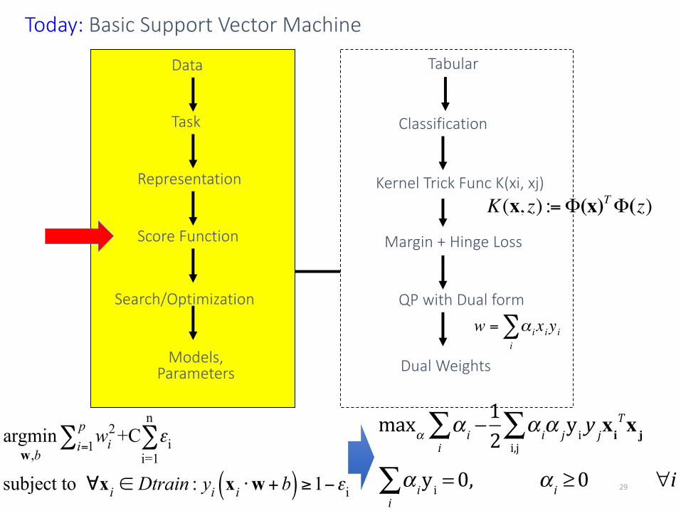
Today: Basic Support Vector Machine
Classification
Kernel Trick Func K(xi, xj)
Margin + Hinge Loss
QP with Dual form
Dual Weights
Task
Representation
Score Function
Search/Optimization
Models, Parameters
€
w = α ixiyii∑
argminw,b
wi2
i=1p∑ +C εi
i=1
n
∑
subject to ∀xi ∈ Dtrain : yi xi ⋅w+b( ) ≥1−εi
K(x, z) :=Φ(x)TΦ(z)
3
maxα α i −i∑ 1
2 α iα jyi y ji,j∑ xi
Txj
α iyi =0i∑ , α i ≥0 ∀i
Data Tabular

Today
qSupport Vector Machine (SVM)ü History of SVM ü Large Margin Linear Classifier ü Define Margin (M) in terms of model parameterü Optimization to learn model parameters (w, b) ü Linearly Non-separable caseü Optimization with dual form ü Nonlinear decision boundary ü Multiclass SVM
11/10/20 Dr. Yanjun Qi / UVA 4

History of SVM
• SVM is inspired from statistical learning theory [3]• SVM was first introduced in 1992 [1]
• SVM becomes popular because of its success in handwritten digit recognition (1994)• 1.1% test error rate for SVM. • The same as the error rates of a carefully constructed neural network, LeNet 4.
• Section 5.11 in [2] or the discussion in [3] for details
• Regarded as an important example of “kernel methods”, arguably the hottest area in machine learning 20 years ago
11/10/20 Dr. Yanjun Qi / UVA 5
[1] B.E. Boser et al. A Training Algorithm for Optimal Margin Classifiers. Proceedings of the Fifth Annual Workshop on Computational Learning Theory 5 144-152, Pittsburgh, 1992.
[2] L. Bottou et al. Comparison of classifier methods: a case study in handwritten digit recognition. Proceedings of the 12th IAPR International Conference on Pattern Recognition, vol. 2, pp. 77-82, 1994.
[3] V. Vapnik. The Nature of Statistical Learning Theory. 2nd edition, Springer, 1999.
Theoretically sound /
Impactful

Handwritten digit recognition
11/10/20 Dr. Yanjun Qi / UVA 6

Mixed National Institute of Standards and Technology (MNIST) • Is a database and evaluation setup for
handwritten digit recognition• Contains 60,000 training and 10,000 test
instances of hand-written digits, encoded as 28×28 pixel grayscale images
• The data is a re-mix of an earlier NIST dataset in which adults generated the training data and high school students generated the test set
• Lets compare the performance of different methods

MNIST
reserved for final tests only. For these and other reasons, some competitive chal-lenges have been organized in which the labels for test data are hidden and resultsmust be submitted to a remote server for evaluation. In some cases the test dataitself is also hidden, in which case participants must submit executable code.
THE MNIST EVALUATION
To underscore the importance of large benchmark evaluations, consider the MixedNational Institute of Standards and Technology (MNIST) database of handwrittendigits. It contains 60,000 training and 10,000 test instances of hand-written digits,encoded as 283 28 pixel grayscale images. The data is a remix of an earlier NISTdata set in which adults generated the training data and high school students gener-ated the test set. Table 10.1 gives some results on this data. Note that the LeNetconvolutional network (row 5), a deep architecture discussed in Section 10.3, out-performed many standard machine learning techniques, even in 1998.
The lower half of the table shows the results of methods that augment the train-ing set with synthetic distortions of the input images. The use of transformations tofurther extend the size of an already large data set is an important technique indeep learning. Large networks, with more parameters, have high representationalcapacity. Plausible synthetic distortion of the data multiplies the amount of dataavailable, preventing overfitting and helping the network to generalize. Of course,
Table 10.1 Summary of Performance on the MNIST Evaluation
ClassifierTest ErrorRate (%) References
Linear classifier (1-layer neural net) 12.0 LeCun et al. (1998)K-nearest-neighbors, Euclidean (L2) 5.0 LeCun et al. (1998)2-Layer neural net, 300 hidden units, meansquare error
4.7 LeCun et al. (1998)
Support vector machine, Gaussian kernel 1.4 MNIST WebsiteConvolutional net, LeNet-5 (no distortions) 0.95 LeCun et al. (1998)
Methods using distortions
Virtual support vector machine, deg-9polynomial, (2-pixel jittered and deskewing)
0.56 DeCoste and Scholkopf(2002)
Convolutional neural net (elastic distortions) 0.4 Simard, Steinkraus, and Platt(2003)
6-Layer feedforward neural net (on GPU)(elastic distortions)
0.35 Ciresan, Meier, Gambardella,and Schmidhuber (2010)
Large/deep convolutional neural net(elastic distortions)
0.35 Ciresan, Meier, Masci, MariaGambardella, andSchmidhuber (2011)
Committee of 35 convolutional networks(elastic distortions)
0.23 Ciresan, Meier, andSchmidhuber (2012)
42110.1 Deep Feedforward Networks
Applications of SVMs
11/10/20 Dr. Yanjun Qi / UVA 9
• Computer Vision• Text Categorization• Ranking (e.g., Google searches)• Handwritten Character Recognition• Time series analysis• Bioinformatics• ……….
àLots of very successful applications!!!

Early History
• In 1950 English mathematician Alan Turing wrote a landmark paper titled “Computing Machinery and Intelligence” that asked the question: “Can machines think?”
• Further work came out of a 1956 workshop at Dartmouth sponsored by John McCarthy. In the proposal for that workshop, he coined the phrase a “study of artificial intelligence”
• 1950s• Samuel’s checker player : start of machine learning• Selfridge’s Pandemonium
• 1952-1969: Enthusiasm: Lots of work on neural networks
• 1970s: Expert systems, Knowledge bases to add on rule-based inference
11/10/20 Yanjun Qi / UVA CS 10Adapted From Prof. Raymond J. Mooney’s slides

Early History• 1980s :• Advanced decision tree and rule learning• Valiant’s PAC Learning Theory
• 1990s: • Reinforcement learning (RL)• Ensembles: Bagging, Boosting, and Stacking• Bayes Net learning• Convolutional neural network (CNN) and Recurrent neural network (RNN) were
invented
• 2000s• Support vector machines (becoming popular and dominating)• Kernel methods• Graphical models• Statistical relational learning• Transfer learning• Sequence labeling• Collective classification and structured outputs11/10/20
Yanjun Qi / UVA CS 11
Adapted From Prof. Raymond J. Mooney’s slides

12
Deep LearningDeep Reinforcement Learning
Generative Adversarial Network (GAN)
• 1952-1969 Enthusiasm: Lots of work on neural networks• 1990s: Convolutional neural network (CNN) and Recurrent neural network (RNN) were invented
Y. LeCun, L. Bottou, Y. Bengio, and P. Haffner, Gradient-based learning applied to document recognition, Proceedings of the IEEE 86(11):
2278–2324, 1998.

Reason of the recent breakthroughs of deep learning:
Plenty of (Labeled) Data
Advanced Computer
Architecture that fits DNNs
Powerful DNN platforms /
Libraries
13

A Dataset for binaryclassification
• Data/points/instances/examples/samples/records: [ rows ]• Features/attributes/dimensions/independent
variables/covariates/predictors/regressors: [ columns, except the last] • Target/outcome/response/label/dependent variable: special column to be
predicted [ last column ]
11/10/20 Dr. Yanjun Qi / UVA 14
Output as Binary Class:
only two possibilities
Today
qSupport Vector Machine (SVM)ü History of SVM ü Large Margin Linear Classifier ü Define Margin (M) in terms of model parameterü Optimization to learn model parameters (w, b) ü Linearly Non-separable caseü Optimization with dual form ü Nonlinear decision boundary ü Multiclass SVM
11/10/20 Dr. Yanjun Qi / UVA 15
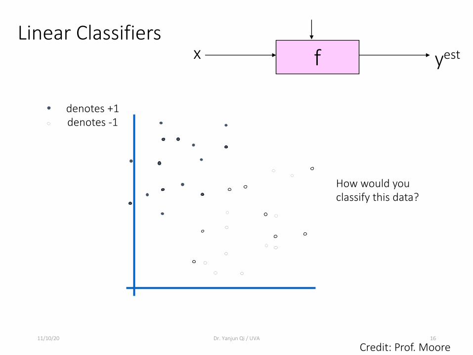
Linear Classifiers
11/10/20 Dr. Yanjun Qi / UVA 16
f x yest
denotes +1denotes -1
How would you classify this data?
Credit: Prof. Moore

Linear Classifiers
11/10/20 Dr. Yanjun Qi / UVA 17
f x yest
denotes +1denotes -1
How would you classify this data?
Credit: Prof. Moore

Linear Classifiers
11/10/20 Dr. Yanjun Qi / UVA 18
f x yest
denotes +1denotes -1
How would you classify this data?
Credit: Prof. Moore

Linear Classifiers
11/10/20 Dr. Yanjun Qi / UVA 19
f x yest
denotes +1denotes -1
How would you classify this data?
Credit: Prof. Moore

Linear Classifiers
11/10/20 Dr. Yanjun Qi / UVA 20
f x yest
denotes +1denotes -1
Any of these would be fine..
..but which is best?
Credit: Prof. Moore

Classifier Margin
11/10/20 Dr. Yanjun Qi / UVA 21
f x yest
denotes +1denotes -1 Define the margin of
a linear classifier as the width that the boundary could be increased by before hitting a datapoint.
Credit: Prof. Moore

Maximum Margin
11/10/20 Dr. Yanjun Qi / UVA 22
f x yest
denotes +1denotes -1 The maximum
margin linear classifier is the linear classifier with the, maximum margin.This is the simplest kind of SVM (Called an LSVM)
Linear SVM
Credit: Prof. Moore

Maximum Margin
11/10/20 Dr. Yanjun Qi / UVA 23
f x yest
denotes +1denotes -1 The maximum
margin linear classifier is the linear classifier with the, maximum margin.This is the simplest kind of SVM (Called an LSVM)
Support Vectors are those datapoints that the margin pushes up against
Linear SVM
x2
x1
Credit: Prof. Moore

Maximum Margin
11/10/20 Dr. Yanjun Qi / UVA 24
f x yest
denotes +1denotes -1 The maximum
margin linear classifier is the linear classifier with the, maximum margin.This is the simplest kind of SVM (Called an LSVM)
Support Vectors are those datapoints that the margin pushes up against
Linear SVM
f(x,w,b) = sign(wTx + b)x2
x1
Credit: Prof. Moore

Max margin classifiers
11/10/20 Dr. Yanjun Qi / UVA 25
• Instead of fitting all points, focus on boundary points
• Learn a boundary that leads to the largest margin from both sets of points
From all the possible boundary lines, this leads to the largest margin on both sides
x2
x1
Credit: Prof. Moore
f(x,w,b) = sign(wTx + b)

Max margin classifiers
11/10/20 Dr. Yanjun Qi / UVA 26
• Instead of fitting all points, focus on boundary points
• Learn a boundary that leads to the largest margin from points on both sides
}}
D
DWhy MAX margin?
• Intuitive, ‘makes sense’
• Some theoretical support (using VC dimension)
• Works well in practice
x2
x1
Credit: Prof. Moore

Thank you
11/10/20 27
Thank You

UVA CS 4774: Machine Learning
S4: Lecture 20: Support Vector Machine (Basics)
Dr. Yanjun Qi
University of VirginiaDepartment of Computer Science
Module II
Today: Basic Support Vector Machine
Classification
Kernel Trick Func K(xi, xj)
Margin + Hinge Loss
QP with Dual form
Dual Weights
Task
Representation
Score Function
Search/Optimization
Models, Parameters
€
w = α ixiyii∑
argminw,b
wi2
i=1p∑ +C εi
i=1
n
∑
subject to ∀xi ∈ Dtrain : yi xi ⋅w+b( ) ≥1−εi
K(x, z) :=Φ(x)TΦ(z)
29
maxα α i −i∑ 1
2 α iα jyi y ji,j∑ xi
Txj
α iyi =0i∑ , α i ≥0 ∀i
Data Tabular
Today
q Supervised Classification q Support Vector Machine (SVM)
ü History of SVM ü Large Margin Linear Classifier ü Define Margin (M) in terms of model parameterü Optimization to learn model parameters (w, b) ü Linearly Non-separable caseü Optimization with dual form ü Nonlinear decision boundary ü Multiclass SVM
11/10/20 Dr. Yanjun Qi / UVA 30

Max margin classifiers
11/10/20 Dr. Yanjun Qi / UVA 31
• Instead of fitting all points, focus on boundary points
• Learn a boundary that leads to the largest margin from points on both sides
}}
D
DThat is why Also known as linear support vector machines (SVMs)
These are the vectors supporting the boundary
x2
x1
Credit: Prof. Moore
f(x,w,b) = sign(wTx + b)

11/10/20 Dr. Yanjun Qi / UVA 32

How to represent a Linear Decision Boundary?
11/10/20 Dr. Yanjun Qi / UVA 33

Review : Affine Hyperplanes
• https://en.wikipedia.org/wiki/Hyperplane• Any hyperplane can be given in coordinates as the solution of a single
linear (algebraic ) equation of degree 1.
11/10/20 Dr. Yanjun Qi / UVA 34
Q: How does this connect to linear regression?

11/10/20 Dr. Yanjun Qi / UVA 35

11/10/20 Dr. Yanjun Qi / UVA 36

11/10/20 Dr. Yanjun Qi / UVA 37

Max-margin & Decision Boundary
11/10/20 Dr. Yanjun Qi / UVA 38
Class -1
Class 1
W is a p-dim vector; b is a
scalar
x2
x1

Max-margin & Decision Boundary• The decision boundary should be as far away from the
data of both classes as possible
11/10/20 Dr. Yanjun Qi / UVA 39
Class -1
Class 1
W is a p-dim vector; b is a
scalar

Specifying a max margin classifier
11/10/20 Dr. Yanjun Qi / UVA 40
Predict class +1
Predict class -1wTx+b=+1
wTx+b=0
wTx+b=-1
Classify as +1 if wTx+b >= 1
Classify as -1 if wTx+b <= - 1
Undefined if -1 <wTx+b < 1
Class +1 plane
boundary
Class -1 plane
f(x,w,b) = sign(wTx + b)

Specifying a max margin classifier
11/10/20 Dr. Yanjun Qi / UVA 41
Predict class +1
Predict class -1wTx+b=+1
wTx+b=0
wTx+b=-1
Classify as +1 if wTx+b >= 1
Classify as -1 if wTx+b <= - 1
Undefined if -1 <wTx+b < 1
Is the linear separation assumption realistic?
We will deal with this shortly, but lets assume it for now

Maximizing the margin
11/10/20 Dr. Yanjun Qi / UVA 42
Predict class +1
Predict class -1wTx+b=+1
wTx+b=0
wTx+b=-1
Classify as +1 if wTx+b >= 1
Classify as -1 if wTx+b <= - 1
Undefined if -1 <wTx+b < 1M
• Let us define the width of the margin by M
• How can we encode our goal of maximizing M in terms of our parameters (w and b)?
• Lets start with a few observations See Concrete derivations of M in Extra slides when 2D

11/10/20 Dr. Yanjun Qi / UVA 43
Concrete derivations of M when X is 1D
Length of the vector

11/10/20 Dr. Yanjun Qi / UVA 44

Finding the optimal parameters
11/10/20 Dr. Yanjun Qi / UVA 45
Predict class +1
Predict class -1wTx+b=+1
wTx+b=0
wTx+b=-1
Mx+
x-
€
M =2wTw
We can now search for the optimal parameters by finding a solution that:
1. Correctly classifies all points
2. Maximizes the margin (or equivalently minimizes wTw)
Several optimization methods can be used: Gradient descent, OR SMO (see extra slides)

Today
q Support Vector Machine (SVM)ü History of SVM ü Large Margin Linear Classifier ü Define Margin (M) in terms of model parameterü Optimization to learn model parameters (w, b) ü Linearly Non-separable caseü Optimization with dual form ü Nonlinear decision boundary ü Practical Guide
11/10/20 Dr. Yanjun Qi / UVA 46

Optimization Step i.e. learning optimal parameter for SVM
11/10/20 Dr. Yanjun Qi / UVA 47
Predict class +1
Predict class -1wTx+b=+1
wTx+b=0
wTx+b=-1
Mx+
x-
€
M =2wTw
f(x,w,b) = sign(wTx + b)

Optimization Step i.e. learning optimal parameter for SVM
11/10/20 Dr. Yanjun Qi / UVA 48
Predict class +1
Predict class -1wTx+b=+1
wTx+b=0
wTx+b=-1
Mx+
x-
€
M =2wTw
Min (wTw)/2subject to the following constraints:
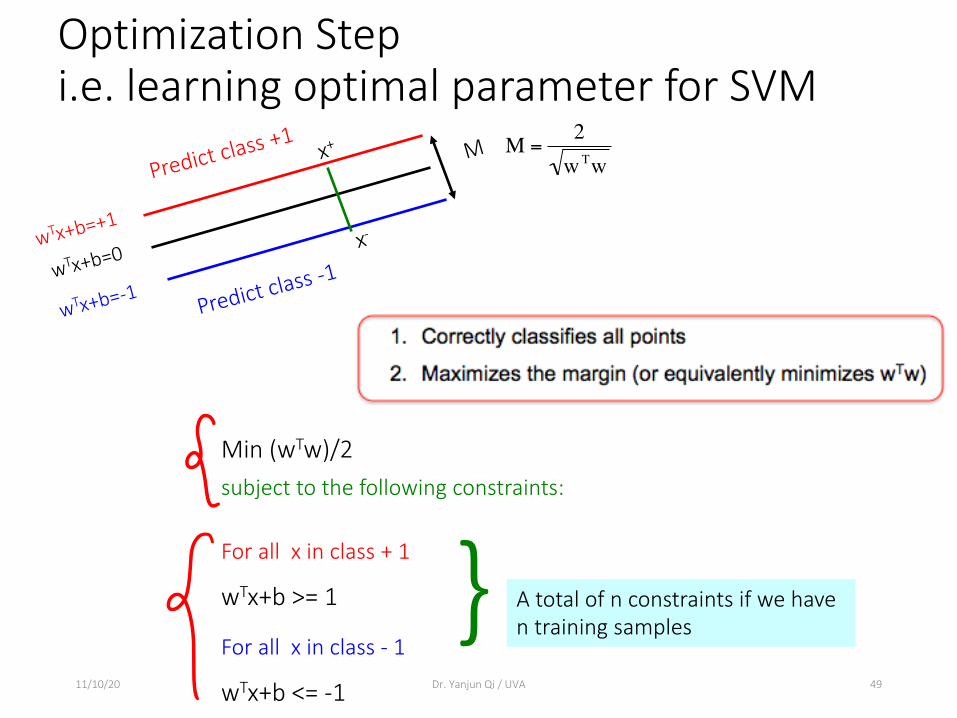
Optimization Step i.e. learning optimal parameter for SVM
11/10/20 Dr. Yanjun Qi / UVA 49
Predict class +1
Predict class -1wTx+b=+1
wTx+b=0
wTx+b=-1
Mx+
x-
€
M =2wTw
Min (wTw)/2 subject to the following constraints:
For all x in class + 1
wTx+b >= 1
For all x in class - 1
wTx+b <= -1
} A total of n constraints if we have n training samples

Optimization Reformulation
11/10/20 Dr. Yanjun Qi / UVA 50
Min (wTw)/2 subject to the following constraints:
For all x in class + 1
wTx+b >= 1
For all x in class - 1
wTx+b <= -1
} A total of n constraints if we have n input samples
f(x,w,b) = sign(wTx + b)
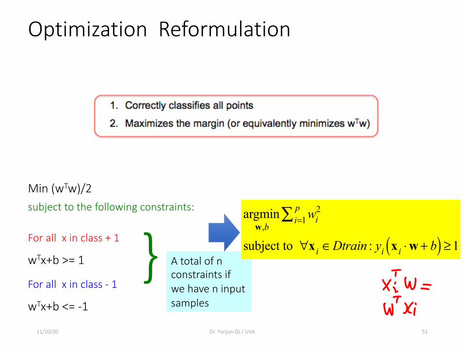
Optimization Reformulation
11/10/20 Dr. Yanjun Qi / UVA 51
Min (wTw)/2 subject to the following constraints:
For all x in class + 1
wTx+b >= 1
For all x in class - 1
wTx+b <= -1
} A total of n constraints if we have n input samples
argminw,b
wi2
i=1p∑
subject to ∀x i ∈Dtrain : yi x i ⋅w + b( ) ≥1

Optimization Reformulation
11/10/20 Dr. Yanjun Qi / UVA 52
Min (wTw)/2 subject to the following constraints:
For all x in class + 1
wTx+b >= 1
For all x in class - 1
wTx+b <= -1
} A total of n constraints if we have n input samples
argminw,b
wi2
i=1p∑
subject to ∀x i ∈Dtrain : yi wT x i + b( ) ≥1
Quadratic Objective
Quadratic programming i.e., - Quadratic objective - Linear constraints
f(x,w,b) = sign(wTx + b)

Today: Basic Support Vector Machine
Classification
Kernel Trick Func K(xi, xj)
Margin + Hinge Loss
QP with Dual form
Dual Weights
Task
Representation
Score Function
Search/Optimization
Models, Parameters
€
w = α ixiyii∑
argminw,b
wi2
i=1p∑ +C εi
i=1
n
∑
subject to ∀xi ∈ Dtrain : yi xi ⋅w+b( ) ≥1−εi
K(x, z) :=Φ(x)TΦ(z)
53
maxα α i −i∑ 1
2 α iα jyi y ji,j∑ xi
Txj
α iyi =0i∑ , α i ≥0 ∀i
Data Tabular

What Next?
q Support Vector Machine (SVM)ü History of SVM ü Large Margin Linear Classifier ü Define Margin (M) in terms of model parameterü Optimization to learn model parameters (w, b) ü Linearly Non-separable case (soft SVM)ü Optimization with dual form ü Nonlinear decision boundary ü Practical Guide
11/10/20 Dr. Yanjun Qi / UVA 54

Thank you
11/10/20 55
Thank You

References
• Big thanks to Prof. Ziv Bar-Joseph and Prof. Eric Xing @ CMU for allowing me to reuse some of his slides• Elements of Statistical Learning, by Hastie, Tibshirani and Friedman• Prof. Andrew Moore @ CMU’s slides• Tutorial slides from Dr. Tie-Yan Liu, MSR Asia• A Practical Guide to Support Vector Classification Chih-Wei Hsu,
Chih-Chung Chang, and Chih-Jen Lin, 2003-2010 • Tutorial slides from Stanford “Convex Optimization I — Boyd &
Vandenberghe
11/10/20 Dr. Yanjun Qi / UVA CS 56

EXTRA
11/10/20 Dr. Yanjun Qi / UVA 57
Concrete derivations of M in Extra slides when X is 2D

How to define the width of the margin by M (EXTRA)
11/10/20 Dr. Yanjun Qi / UVA 58
Predict class +1
Predict class -1wTx+b=+1
wTx+b=0
wTx+b=-1
Classify as +1 if wTx+b >= 1
Classify as -1 if wTx+b <= - 1
Undefined if -1 <wTx+b < 1M
• Lets define the width of the margin by M
• How can we encode our goal of maximizing M in terms of our parameters (w and b)?
• Lets start with a few obsevrations Concrete derivations of M see Extra

11/10/20 Dr. Yanjun Qi / UVA 59
The gradient points in the direction of the greatest rate of increase of the function and its magnitude is the slope of the graph in that direction

Margin M
11/10/20 Dr. Yanjun Qi / UVA 60

11/10/20 Dr. Yanjun Qi / UVA 61
• wT x+ + b = +1
• wT x- + b = -1
• M = | x+ - x- | = ?

Maximizing the margin: observation-1
11/10/20 Dr. Yanjun Qi / UVA 62
Predict class +1
Predict class -1wTx+b=+1
wTx+b=0
wTx+b=-1
M
• Observation 1: the vector w is orthogonal to the +1 plane
• Why?
Corollary: the vector w is orthogonal to the -1 plane

Maximizing the margin: observation-1
11/10/20 Dr. Yanjun Qi / UVA 63
Predict class +1
Predict class -1wTx+b=+1
wTx+b=0
wTx+b=-1
Classify as +1 if wTx+b >= 1
Classify as -1 if wTx+b <= - 1
Undefined if -1 <wTx+b < 1
M
• Observation 1: the vector w is orthogonal to the +1 plane
• Why?
Let u and v be two points on the +1 plane, then for the vector defined by u and v we have wT(u-v) = 0
Corollary: the vector w is orthogonal to the -1 plane
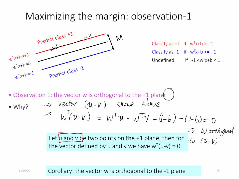
Maximizing the margin: observation-1
11/10/20 Dr. Yanjun Qi / UVA 64
Predict class +1
Predict class -1wTx+b=+1
wTx+b=0
wTx+b=-1
Classify as +1 if wTx+b >= 1
Classify as -1 if wTx+b <= - 1
Undefined if -1 <wTx+b < 1
M
• Observation 1: the vector w is orthogonal to the +1 plane
• Why?
Let u and v be two points on the +1 plane, then for the vector defined by u and v we have wT(u-v) = 0
Corollary: the vector w is orthogonal to the -1 plane

Review :Vector Product, Orthogonal, and Norm
11/10/20 Dr. Yanjun Qi / UVA 65
For two vectors x and y,
xTy
is called the (inner) vector product.
The square root of the product of a vector with itself,
is called the 2-norm ( |x|2 ), can also write as |x|
x and y are called orthogonal if
xTy = 0

Observation 1 è Review : Orthogonal
11/10/20 Dr. Yanjun Qi / UVA 66
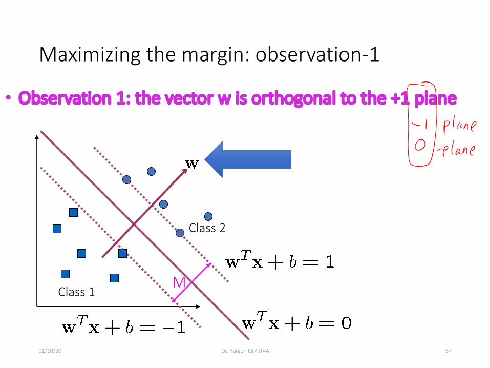
Maximizing the margin: observation-1
• Observation 1: the vector w is orthogonal to the +1 plane
11/10/20 Dr. Yanjun Qi / UVA 67
Class 1
Class 2
M
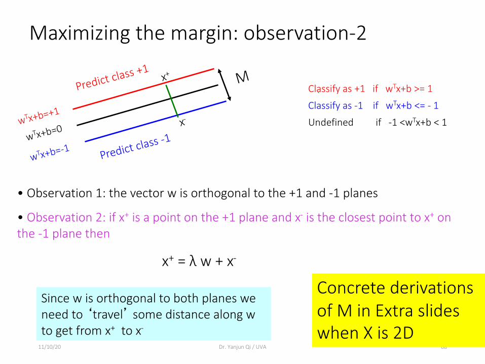
Maximizing the margin: observation-2
11/10/20 Dr. Yanjun Qi / UVA 68
Predict class +1
Predict class -1wTx+b=+1
wTx+b=0
wTx+b=-1
Classify as +1 if wTx+b >= 1
Classify as -1 if wTx+b <= - 1
Undefined if -1 <wTx+b < 1
M
• Observation 1: the vector w is orthogonal to the +1 and -1 planes
• Observation 2: if x+ is a point on the +1 plane and x- is the closest point to x+ on the -1 plane then
x+ = λ w + x-
x+
x-
Since w is orthogonal to both planes we need to ‘travel’ some distance along w to get from x+ to x-
Concrete derivations of M in Extra slides when X is 2D

Putting it together
11/10/20 Dr. Yanjun Qi / UVA 69
• wT x+ + b = +1
• wT x- + b = -1
• M = | x+ - x- | = ?
• x+ = λ w + x-
Concrete derivations of M in Extra slides when X is 2D

Putting it together
11/10/20 Dr. Yanjun Qi / UVA 70
Predict class +1
Predict class -1wTx+b=+1
wTx+b=0
wTx+b=-1
M
• wT x+ + b = +1
• wT x- + b = -1
• x+ = λ w + x-
• | x+ - x- | = M
x+
x-
We can now define M in terms of w and b
11/10/20 Dr. Yanjun Qi / UVA 71
Concrete derivations of M in Extra slides when X is 2D

Putting it together
11/10/20 Dr. Yanjun Qi / UVA 72
Predict class +1
Predict class -1wTx+b=+1
wTx+b=0
wTx+b=-1
M
• wT x+ + b = +1
• wT x- + b = -1
• x+ = λw + x-
• | x+ - x- | = M
x+
x-
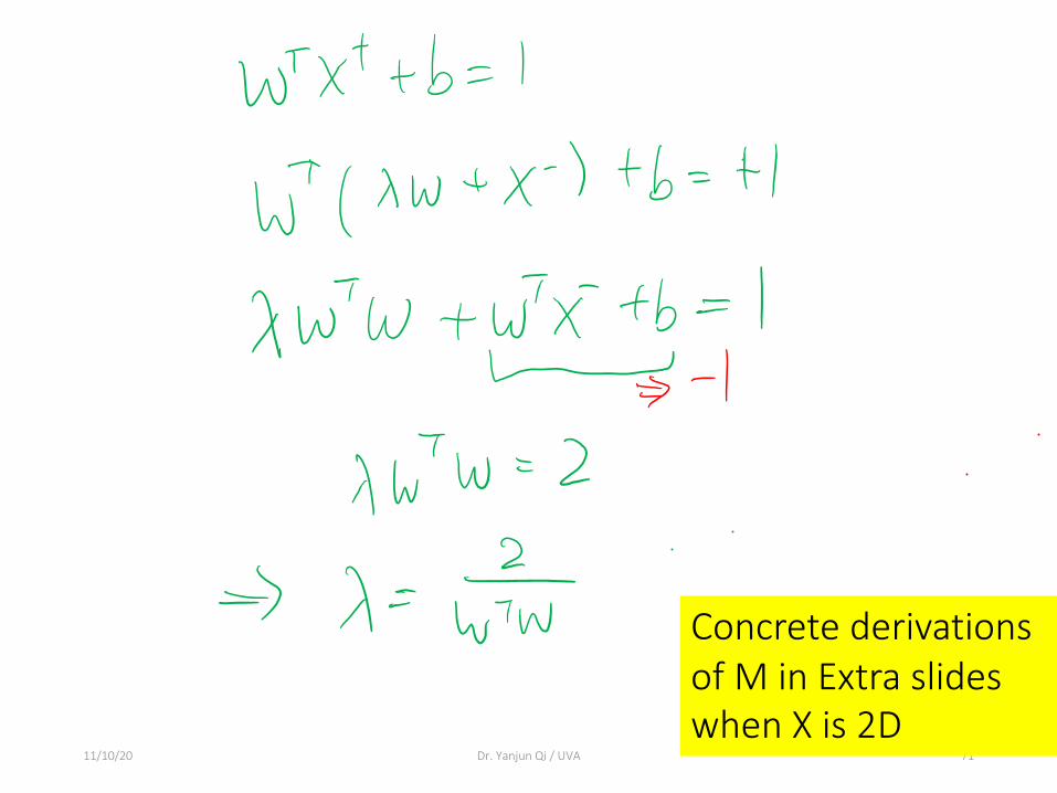
We can now define M in terms of w and b
wT x+ + b = +1
=>
wT (λw + x-) + b = +1=>
wTx- + b + λwTw = +1
=>
-1 + λwTw = +1
=>
λ = 2/wTw

Putting it together
11/10/20 Dr. Yanjun Qi / UVA 73
Predict class +1
Predict class -1wTx+b=+1
wTx+b=0
wTx+b=-1
M
• wT x+ + b = +1
• wT x- + b = -1
• x+ = λ w + x-
• | x+ - x- | = M
• λ = 2/wTw
x+
x-
We can now define M in terms of w and b
M = |x+ - x-|
=>
=>
M =| λw |= λ | w |= λ wTw
€
M = 2 wTwwTw
=2wTw