USPAS 2008, University of Maryland

PHASE SPACE TOMOGRAPHY LECTURE NOTES1

Prepared By

Diktys Stratakis

Instructor for the UMER course for USPAS 2008

Institute for Research in Electronics and Applied Physics,

University of Maryland, College Park, MD 20742

1All lecture notes are from the following Dissertation: D. Stratakis, Ph.D.

Dissertation, “Tomographic Measurement of the Phase Space Distribution of a Space-

Charge-Dominated Beam”, University of Maryland, 2008

© Copyright by

Diktys Stratakis

2008

iii

1

Tomography Theory

Measurement of the transverse phase space distribution is an important tool to

understand transverse particle dynamics in accelerators. Standard methods that are

commonly used in the accelerator community to map the beam phase space (such as

the quadrupole scan, pepper pot, and slit wire scan) were briefly reviewed in Chap. 1

and as it was evident they had some limitations. Therefore, it is advantageous to

develop new methods to accurately reconstruct the beam phase space.

This chapter describes how to measure the transverse phase space distribution

by combining the ideas of quadrupole-scanning with Tomographic image techniques.

Prior work demonstrated that it is possible to map the beam phase space by measuring

spatial projections of the beam. However, these previous methods were applied to

relativistic beams with no space-charge. In this chapter we discuss the difficulties

arising in cases were space-charge is present and demonstrate an algorithm for

Tomographic phase space mapping for intense space-charge dominated beams.

The outline of this chapter is as follows: In Sec. 2.1 we briefly review the

basic beam theory, discuss the motion of a single beam particle and define space-

charge. In Sec. 2.2 we review the tomography algorithm and its relations to the phase

space measurement for beams without space-charge. In Sec. 2.3 we show the

extension algorithm to use tomography to beams with space-charge. In Sec. 2.4 we

discuss the modifications we do to apply the diagnostic for our experiments. Finally,

we review the image analysis software for tomography and show a step by step

example where we describe how to use it to reconstruct the beam phase-space.

2

2.1 Basic Theory

A beam consists of a group of particles that have small energy spread

compared to their average translational energy, and where the particle transverse

motion is at very small angles with respect to the beam translational orbit. We briefly

review the motion of a single beam particle and discuss the implications when space-

charge is present.

2.1.1 Beam Transfer Matrices

In this section we describe the transverse particle motion at the exit of a beam

transport location, such as a lens or a simple drift segment, relative to the orbit at the

entrance. As discussed in Chap.1 the position of the particle can be represented as a

point in a six dimensional space. Assume that the beam propagates in the z-direction

with a longitudinal momentum and size much higher than the momentum and size in

the transverse directions. Then, the transverse particle orbit at some axial position can

be represented by the four-dimensional vector ' '( , , , )x x y y , where x (or y) is the

transverse displacement from the horizontal plane x (or y). The quantity 'x (or 'y ) is

the angle the particle makes in that plane with respect to the main axis z. In many

practical cases the forces in the x and y directions are independent and we can

calculate the particle motion in x and y separately using the two-dimensional vectors

'( , )x x and '( , )y y , respectively. We shall concentrate our analysis of orbits that are

separable in x and y.

3

Figure 0.1: Layout showing a particle that enters a lens at 0z and exits the lens at 1z .

Consider the motion of a particle along the transverse x-direction in a lens of

length d as shown in Fig. 2.1. If the exit vector is '

1 1( , )x x and the entrance vector is

'

0 0( , )x x then the particle equation of motion is:

2

02

d xx

dzκ= − , (2.1)

where 0F xκ= is the focusing force of the lens assumed to be linear. Equation 2.1

has the following solutions:

'

01 0 0 0

0

cos( ) sin( )x

x x d dκ κκ

= + , (2.2)

' '

1 0 0 0 0 0sin( ) cos( )x x d x dκ κ κ= − + . (2.3)

In matrix notation, the above equations can be written as:

0 0 0 01

0' ' '

1 0 0

0 0 0

1cos( ) sin( )

sin( ) cos( )

d d x xxT

x x xd d

κ κκ

κ κ κ

= = −

. (2.4)

The matrix T is known as the transport matrix of the lens and κ0 is often called the

focusing function and is related to the strength of the lens. For quadrupole magnets

the focusing function is [7]

z

0

'

0

x

x

1

'

1

x

x

0z 1z

MAGNET d

4

0

qg

m cκ

γβ= , (2.5)

where g is the quadrupole field gradient; q, m , and c are the particle charge, mass and

speed of light, respectively. In practice, it is common to model the quadrupole by

using a “hard-edge” approximation where the magnetic field is constant inside the

quadrupole over a certain length, known as effective lengtheff

L , and drops to zero

outside. From Eq. 2.2 we see that particles oscillate harmonically when traveling

through the lens. Those oscillations are known as betatron oscillations with betatron

wavelength, 0βλ , which for our case is 0 02 /βλ π κ= .

As it easy follows from Eq. 2.4 when the beam is passing through a drift

section ( 0κ is zero), the transport matrix becomes

1

0 1

dT

=

. (2.6)

Next, we are interested to study the influence of space-charge on the particle motion.

2.1.2 Space-charge Effects on Particle Motion

In the previous chapter we assumed that individual particles are moving only

under the influence of the external focusing forces. However, as the current is

increased the superimposed electric field generated by the particles themselves

becomes non-negligible generating phenomena known as space-charge (see Sec. 1.3).

Space-charge results to a repelling force, SCF , and therefore Eq. 2.1 becomes

2

02 SC

d xx F

dzκ= − + . (2.7)

5

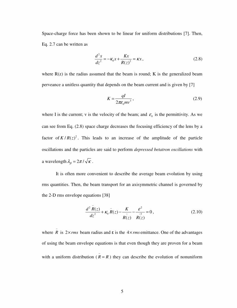
Space-charge force has been shown to be linear for uniform distributions [7]. Then,

Eq. 2.7 can be written as

2

02 2( )

d x Kxx x

dz R zκ κ= − + = , (2.8)

where R(z) is the radius assumed that the beam is round; K is the generalized beam

perveance a unitless quantity that depends on the beam current and is given by [7]

3

02

qIK

mvπε= , (2.9)

where I is the current; v is the velocity of the beam; and 0ε is the permittivity. As we

can see from Eq. (2.8) space charge decreases the focusing efficiency of the lens by a

factor of 2/ ( )K R z . This leads to an increase of the amplitude of the particle

oscillations and the particles are said to perform depressed betatron oscillations with

a wavelength 2 /βλ π κ= .

It is often more convenient to describe the average beam evolution by using

rms quantities. Then, the beam transport for an axisymmetric channel is governed by

the 2-D rms envelope equations [38]

2 2

0 32

( )( ) 0

( ) ( )

d R z KR z

dz R z R z

εκ

−−

− −+ − − = , (2.10)

where R−

is 2 rms× beam radius and ε is the 4 rms× emittance. One of the advantages

of using the beam envelope equations is that even though they are proven for a beam

with a uniform distribution ( R R−

= ) they can describe the evolution of nonuniform

6

beams as long as they energy, current, rms size and divergence are equivalent to that

of a uniform beam [7, 38].

From Eq. (2.10) we can see that the average behavior of the beam is

determined by three forces: the focusing force, the space charge force and the thermal

pressure force from the emittance. When these forces are balanced

2

0 3( )

( ) ( )

KR z

R z R z

εκ

−

− −= + , (2.11)

and the beam is known as matched. Depending on which of the two terms in the right

side of Eq. (2.11) dominate, the beam is space-charge dominated (2

3

K

R R

ε− −

> ) or

emittance-dominated (2

3

K

R R

ε− −

< ).

Another way to quantify space-charge is by introducing the dimensionless

intensity parameter χ which can be expressed as the ratio of space-charge force to

external focusing force and is given by [39]

2

0

K

R

χκ

−= . (2.12)

If, 0 0.5χ< ≤ the beam is emittance dominated, if 0.5 1χ< < it is space charge

dominated. The betatron wavelength and depressed wavelength can be expressed in

terms of the intensity parameter χ by

1/ 2

0

(1 )β

β

λχ

λ−= − . (2.13)

Clearly, as χ approaches unity the betatron wavelength becomes extremely large.

7

2.2 Tomography for Beams without Space-Charge

We now review the tomography algorithm (Sec. 2.2.1) and show its extension

to reconstruct the beam phase space distribution (Sec. 2.2.2).

2.2.1 Filtered-Backprojection Algorithm

Several algorithms [40] are available to compute high quality reconstructions

from projection data, e. g., Algebraic Reconstruction Technique, Maximum Entropy

Tomography, filtered-backprojection algorithm (FBA), etc. The FBA algorithm is the

most common method to reconstruct a two-dimensional image and is generally

believed that it provides a reconstructed image of high quality with normally

available computer capacity and computational times [40]. This is the algorithm that

we use and hence we describe in detail along the lines below.

8

Figure 0.2: Illustration of the Radon Transform

Suppose that ),( yxf corresponds to a two dimensional distribution. Then the

integral

^

( , ) ( , ) ( cos sin )f t dxdyf x y x y tθ δ θ θ∞ ∞

−∞ −∞

= + −∫ ∫ (2.14)

defines the transverse projection of the distribution ),( yxf along the axis

cos sint x yθ θ= + , placed at an angle θ relative to the x-axis. Such a projection is

known as the Radon transform of the function ),( yxf and is shown in Fig. 2.2. If

( , )F u v is the two-dimensional Fourier transform of the function ),( yxf , then its

inverse Fourier transform is given by

θ f(x,y)

^

( , )f t θ

t

t

s

9

2 ( )( , ) ( , ) j ux vyf x y F u v e dudv

π∞ ∞

+

−∞ −∞

= ∫ ∫ . (2.15)

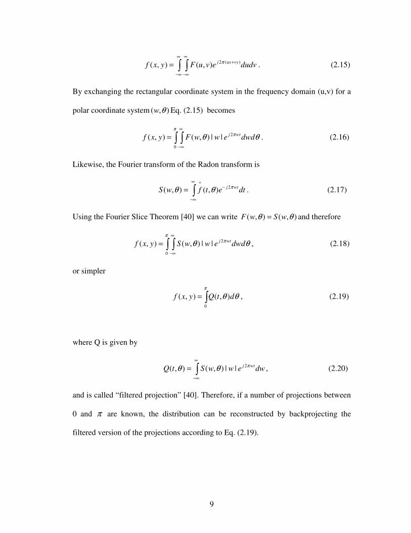
By exchanging the rectangular coordinate system in the frequency domain (u,v) for a

polar coordinate system ),( θw Eq. (2.15) becomes

2

0

( , ) ( , ) | | j wtf x y F w w e dwd

ππθ θ

∞

−∞

= ∫ ∫ . (2.16)

Likewise, the Fourier transform of the Radon transform is

^

2( , ) ( , ) j wtS w f t e dt

πθ θ∞

−

−∞

= ∫ . (2.17)

Using the Fourier Slice Theorem [40] we can write ( , ) ( , )F w S wθ θ= and therefore

2

0

( , ) ( , ) | | j wtf x y S w w e dwd

ππθ θ

∞

−∞

= ∫ ∫ , (2.18)

or simpler

0

( , ) ( , )f x y Q t d

π

θ θ= ∫ , (2.19)

where Q is given by

2( , ) ( , ) | | j wtQ t S w w e dw

πθ θ∞

−∞

= ∫ , (2.20)

and is called “filtered projection” [40]. Therefore, if a number of projections between

0 and π are known, the distribution can be reconstructed by backprojecting the

filtered version of the projections according to Eq. (2.19).

10

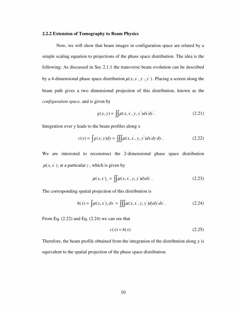
2.2.2 Extension of Tomography to Beam Physics

Now, we will show that beam images in configuration space are related by a

simple scaling equation to projections of the phase space distribution. The idea is the

following: As discussed in Sec 2.1.1 the transverse beam evolution can be described

by a 4-dimensional phase space distribution ' '( , , , )x x y yµ . Placing a screen along the

beam path gives a two dimensional projection of this distribution, known as the

configuration space, and is given by

' ' ' '( , ) ( , , , )g x y x x y y dx dyµ= ∫∫ . (2.21)

Integration over y leads to the beam profiles along x

' ' ' '( ) ( , ) ( , , , )c x g x y dy x x y y dx dy dyµ= =∫ ∫∫∫ . (2.22)

We are interested to reconstruct the 2-dimensional phase space distribution

'( , )z

x xµ at a particular z , which is given by

' ' ' '( , ) ( , , , )z

x x x x y y dydyµ µ= ∫∫ . (2.23)

The corresponding spatial projection of this distribution is

' ' ' ' ' '( ) ( , ) ( , , , )zh x x x dx x x y y dydy dxµ µ= =∫ ∫∫∫ . (2.24)

From Eq. (2.22) and Eq. (2.24) we can see that

( ) ( )c x h x= (2.25)

Therefore, the beam profile obtained from the integration of the distribution along y is

equivalent to the spatial projection of the phase space distribution.

11

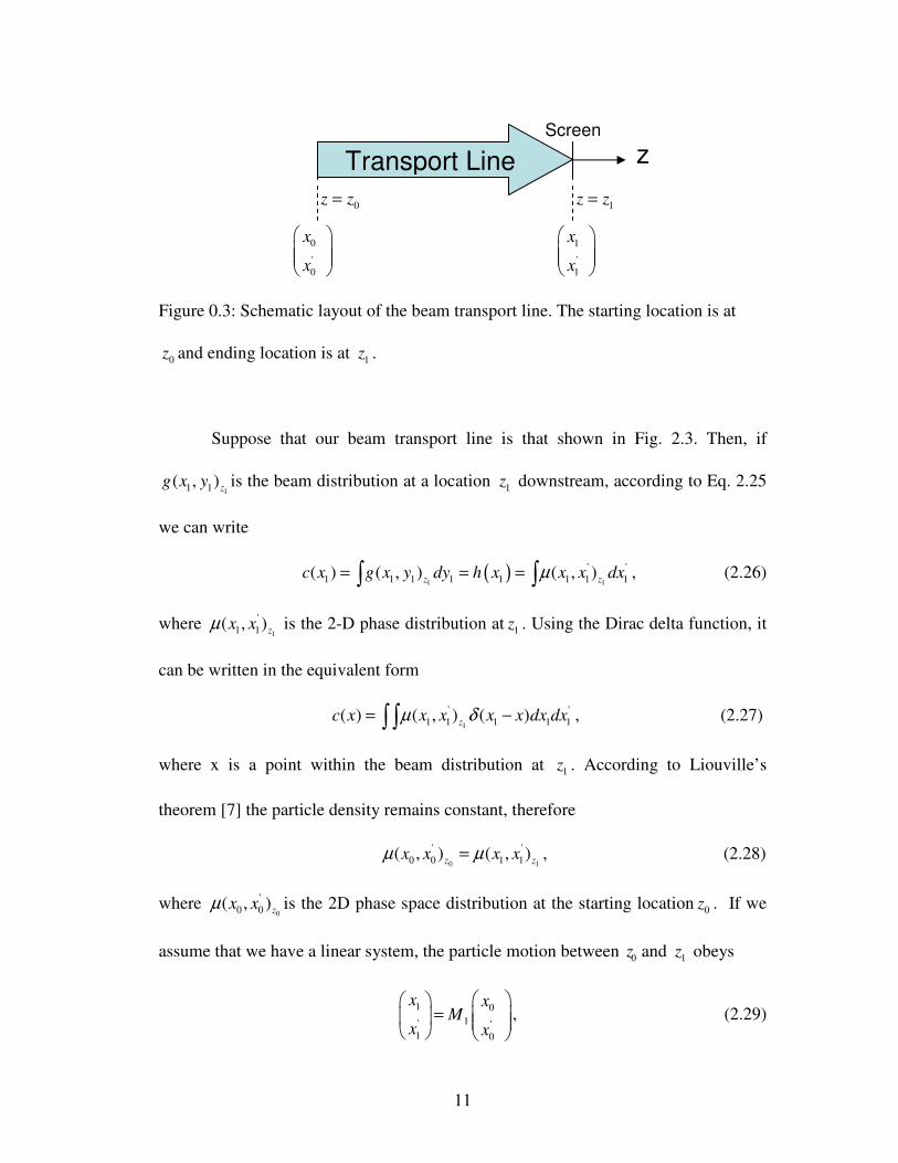
Figure 0.3: Schematic layout of the beam transport line. The starting location is at

0z and ending location is at 1z .

Suppose that our beam transport line is that shown in Fig. 2.3. Then, if

11 1( , )z

g x y is the beam distribution at a location 1z downstream, according to Eq. 2.25

we can write

( )1 1

' '

1 1 1 1 1 1 1 1( ) ( , ) ( , )z z

c x g x y dy h x x x dxµ= = =∫ ∫ , (2.26)

where 1

'

1 1( , )zx xµ is the 2-D phase distribution at 1z . Using the Dirac delta function, it

can be written in the equivalent form

1

' '

1 1 1 1 1( ) ( , ) ( )z

c x x x x x dx dxµ δ= −∫ ∫ , (2.27)

where x is a point within the beam distribution at 1z . According to Liouville’s

theorem [7] the particle density remains constant, therefore

0 1

' '

0 0 1 1( , ) ( , )z zx x x xµ µ= , (2.28)

where 0

'

0 0( , )zx xµ is the 2D phase space distribution at the starting location 0z . If we

assume that we have a linear system, the particle motion between 0z and 1z obeys

1 0

1' '1 0

x xM

x x

=

, (2.29)

Screen

1

'

1

x

x

0

'

0

x

x

0z z= 1z z=

z Transport Line

12

where 11 12

1

21 22

M MM

M M

=

is the transport matrix. Typically the transport line can

consist of drift sections and several lenses. By combining Eq. (2.28) with Eq. (2.29)

we can write:

0

' ' '

0 0 11 0 12 0 0 0( ) ( , ) ( )z

c x x x M x M x x dx dxµ δ= + −∫ ∫ . (2.30)

In order to relate Eq. (2.30) to the Radon transform we define the scaling

factor, s , by [21]

2

12

2

11 MMs += , (2.31)

and the phase space rotation angle θ , by [21]

11

12tanM

M=θ . (2.32)

Now, using Eq. (2.31) and Eq. (2.32), Eq. (2. 30) becomes

0

' ' '

0 0 0 0 0 0

1( ) ( , ) ( cos sin )

zc x x x x x dx dx

sµ δ θ θ ρ= + −∫ ∫ , (2.33)

where sx /=ρ .

Comparing Eq. (2.14) with Eq. (2.33) we can write

0 0

^ ^

( , ) ( / , ) ( / )z zx s sc x sµ ρ θ µ θ= = . (2.34)

From Eq. (2.34) we can deduce that a simple scaling equation relates the

spatial beam projections to the Radon transform,0

^

( / , )zx sµ θ of the transverse phase

space. This is a very useful result since the beam spatial distribution can be easily

obtained in experiments, e.g., using a phosphor screen. Both, scaling factor and

13

angles of the projection can be easily calculated from the beamline overall transport

matrix and are functions of the magnet focusing.

The complete beam tomography procedure can therefore be as follows:

For a given magnet setting:

1. Calculate the transport matrix M1 between 0z and 1z

2. At point 1z z= , get the beam distribution ( , )g x y and calculate the profile by

using Eq. 2.26.

3. Calculate the rotation angle and scaling factor by using Eq. 2.31 and Eq. 2.32

4. Relate the beam profile to the Radon transform by scaling the profile

vertically by s and horizontally by /x s according to Eq. 2.34

5. Filter the projections by calculating Q from Eq. 2.20

6. Change the magnet setting and repeat steps 1-5

At the end of the scan integrate the filtered projections, Q, over the rotation angle by

using Eq. 2.19.

2.2.3 Example: Tomography with Quadrupoles

In the previous section we studied theoretically how to relate the beam

profiles to the Radon transform of the phase space. Here we are interested to

demonstrate an example of this process. Suppose that the transport line of Fig. 2.3

consist of a quadruple lens of effective length 1L followed by a drift section of

length 2L .Such configuration is illustrated in Fig. 2.4.

14

Our goal is to measure the phase space at 0z by collecting beam profiles at

1z .We will follow step by step the process described in section 2.2.2. First, we have

to calculate the transfer matrix 1M . For our beamline

1 D QM M M= , (2.35)

where D

M is the transport matrix of the drift section given by Eq. (2.6) and Q

M is

the transport matrix of the quadrupole given by Eq. (2.4). My multiplying those

matrices we get

2 0 0 1 0 1 0 1 2 0 1

01

0 0 1 0 1

1sin( ) cos( ) sin( ) cos( )

sin( ) cos( )

L L L L L LM

L L

κ κ κ κ κκ

κ κ κ

− + +

= −

.(2.36)

Next, we can use this information to get the rotation angle and scaling factors. Hence,

by using Eq. (2.32) the rotation angle is

0 1 2 0 1

01

2 0 0 1 0 1

1sin( ) cos( )

tan ( )in( ) cos( )

L L L

L s L L

κ κκ

θκ κ κ

−

+

=− +

, (2.37)

and from Eq. (2.31) the scaling factor is

2 2

0 1 2 0 1 2 0 0 1 0 1

0

1[ sin( ) cos( )] [ sin( ) cos( )]s L L L L L Lκ κ κ κ κ

κ= + + − + .(2.38)

In the analysis we assumed focusing quadrupoles (κ >0); however, the same set of

equations can be used for defocusing quadrupoles by just replacing 0κ with 0κ− . In

15

typical experiments, quadruple and drift lengths are fixed, therefore the projection

angle and scaling factor are only functions of the magnet strength 0κ .

Figure 0.4: Schematic layout of the beamline between 0z and 1z . The arrows at the

bottom represent the transport matrices.

Filtered projections, Q, at 1z for different focusing strengths can be used to

derive the phase-space distribution. In Fig. 2.5 we show the procedure to obtain those

projections for three different magnet settings. First, we have to obtain the beam

distribution ( , )g x y at 1z for each case. We can do so by placing an imaging

diagnostic there. Figure 2.5 (first row) shows beam distributions ( , )g x y at 1z for

three different magnet settings (indicated at the top of the photo). Figure 2.5 (second

row) illustrates the corresponding transport matrix, 1M , (from Eq. 2.36) were we

assumed 1 3.72L = cm, 2 12.28L = cm and 43.61 10−× /G Acm for the quadrupole

length, drift length and field gradient, respectively. From the beam distributions and

Eq. 2.26 we calculate the beam profiles ( )c x (Fig. 2.5, third row). Now we have to

scale those profiles and relate them to the Radon transform of the phase space (see

Screen

1

'

1

x

x

0

'

0

x

x

1z z=

z Q

1L 2L

0z z=

QM

DM

16

Eq. 2.34). Our results are demonstrated in the fourth row of Fig. 2.5 as well as the

value of the corresponding rotation angle and scaling factor (calculated from Eq. 2.37

and Eq. 2.38). Finally, we have to filter those profiles by using Eq. 2.20. Such profiles

are illustrated at the last column of Fig. 2.5. The final step is to integrate over the

whole range of angles (Eq. 2.19). As we will show in the next chapter, usually a large

number of projections within the whole (0, 180) degree range is necessary to do an

accurate reconstruction. In our example we had to collect 87 projections by varying

the strength of the magnet from 0 371.8κ = m-2

to 0 230.1κ = − m-2

and our

reconstructed phase space is shown in Fig. 2.6.

17

Figure 0.5: Example demonstrating the procedure to obtain projections of the phase-

space distribution.

0

0.71

169.7

s

θ

=

= 0

0.43

20.2

s

θ

=

= 0

1.50

6.4

s

θ

=

=

1

0.70 0.12

12.00 0.76M

− =

− 1

0.40 0.14

4.20 0.92M

=

− 1

1.49 0.17

3.48 1.06M

=

0

0.2

0.2

0 -15mm 15mm

-15mm 15mm

2

0 3 5 0 .5 mκ −= 2

0 116.1mκ −= 2

0 91.6mκ −= −

c(x

) µ

(ρ,θ

) g

(x,y

)

0 0 0

Q(ρ

,θ)

18

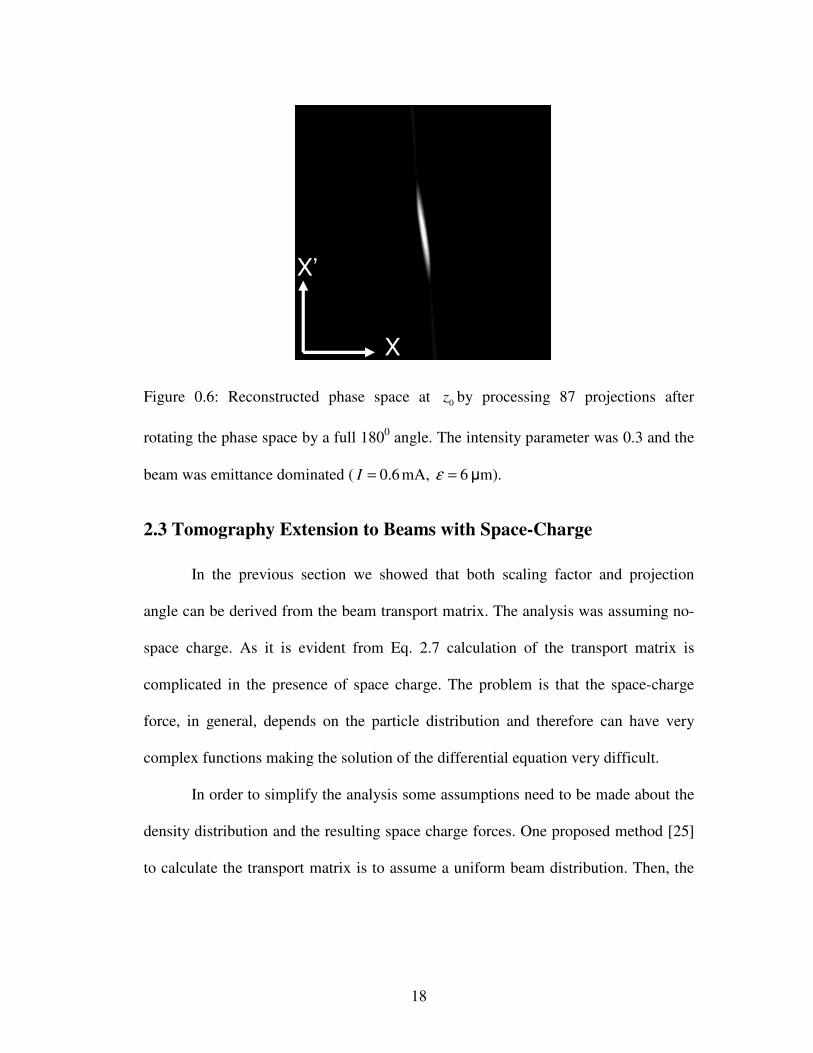
Figure 0.6: Reconstructed phase space at 0z by processing 87 projections after

rotating the phase space by a full 1800 angle. The intensity parameter was 0.3 and the

beam was emittance dominated ( 0.6I = mA, 6ε = µm).

2.3 Tomography Extension to Beams with Space-Charge

In the previous section we showed that both scaling factor and projection

angle can be derived from the beam transport matrix. The analysis was assuming no-

space charge. As it is evident from Eq. 2.7 calculation of the transport matrix is

complicated in the presence of space charge. The problem is that the space-charge

force, in general, depends on the particle distribution and therefore can have very

complex functions making the solution of the differential equation very difficult.

In order to simplify the analysis some assumptions need to be made about the

density distribution and the resulting space charge forces. One proposed method [25]

to calculate the transport matrix is to assume a uniform beam distribution. Then, the

X

X’

19

space charge forces become linear and according to Eq. 2.8 the net focusing strengths

(generalized to a non-symmetric beam) become [7]:

0

2

( )x x

K

X X Yκ κ= −

+, (2.39)

0

2

( )y y

K

Y X Yκ κ= −

+, (2.40)

where 0 0,x y

κ κ are quadrupole focusing strengths defined by Eq. 2.5, and ,X Y are the

2 rms× beam sizes for x and y directions, respectively. Clearly, when space charge is

not significant, only the terms 0 0,x y

κ κ will be used in generating the transfer matrices

and the case becomes equivalent to the discussions in Sec 2.2.2; however, for a more

intense beam the defocusing space charge terms 2

( )

K

X X Y−

+ and

2

( )

K

Y X Y−

+ must

be included in the matrix analysis.

In order to obtain the net focusing strength, knowledge of the beam sizes X

and Y is needed. In typical experiments it’s difficult to place a diagnostic over the

desired transport line to get any information of the detailed evolution of X and Y.

However, assuming no emittance growth we can calculate the beam envelopes by

using Eq 2.10, generalized to non-symmetric distributions and given by [38]

2

0 3

20x

x

KX X

X Y X

εκ′′ + − − =

+, (2.41)

2

0 3

20

y

y

KY Y

X Y Y

εκ′′ + − − =

+. (2.42)

20

In order to solve those differential equations we have to assume some initial

conditions ' '

0 0 0 0( , , , , , )x yX X Y Y ε ε at the starting point 0z . This is a significant

difference with the tomography for beams without space-charge (see Sec. 2.2.2)

where no such assumption was necessary.

To check the validity of our assumptions we compare at 1z the calculated from

the beam envelope and measured from the screen, beam sizes. In case they do not

agree well we adjust the initial conditions and repeat our envelope calculations until

we get a better agreement. Once the evolution of ,X Y with respect of z is known we

calculate the net focusing functions by using Eq. (2.39) and Eq. (2.40). Finally, from

Eq. (2.31) and Eq. (2.32) we calculate the scaling factor and the rotation angle,

respectively.

The complete beam tomography procedure for beams with space-charge is as

follows:

1. Estimate the initial conditions at the starting location 0z .

2. Identify the correct initial conditions at 0z : For each magnet setting, solve the

beam envelope equations and compare the calculated beam size to that from

the measurement. If the two values are not within 10%, estimate new initial

conditions and repeat the process until good agreement is achieved.

3. For each magnet setting solve numerically the envelope equation, get X{z},

Y{z) along the beam line at 0.4 mm (or less) steps, and calculate the focusing

strength for each step by using Eq. 2.39 and Eq. 2.40.

21

4. Use those focusing strengths to calculate the transport matrix (for each step)

and then obtain the total transport matrix by multiplying those matrices. Now

follow the steps 2-5 described in Sec. 2.2.2.

5. Change magnet focusing and repeat steps 3-4.

At the end of the scan integrate the filtered projections, Q, over the rotation angle by

using Eq. 2.19.

2.4 Practical Tomography

2.4.1 Limitations

Phase space tomography requires the beam distribution to be rotated to a full

1800 angle. Often this cannot be achieved by a single magnet because of several

restrictions imposed by the experiment. Such restrictions are listed below:

Beam pipe: The beam size must be kept within a reasonable range when it travels

trough the accelerator in order to avoid the beam hitting the pipe or possible image-

charge effects. Simulations indicate that image forces can have a significant impact

on the beam dynamics, since it can cause emittance growth.

Screen size: Tomography relies on the beam distribution captured on the screen.

Therefore, the beam size at the measurement point must be controlled to remain

within the phosphor screen.

Magnet strength: In practice, the magnet strength is limited by the power supplies or

hardware used. For instance, such a restriction can be the magnet current which on

UMER cannot exceed ± 3.5 A. Additionally, operating at high quadrupole currents

can destroy the quadrupole printed circuit.

22

Therefore, given those limitations, in some cases one quadrupole is not

enough for a full 1800 rotation of the phase-space. For instance, on UMER we have

to employ three and sometimes four quadrupoles to ensure high quality phase spaces.

Such configuration not only ensures a full rotation of the phase space but also

guarantees that the beam remains far from the beam pipe and therefore the effect of

image forces is negligible. Details about the UMER configuration will be discussed in

the next section.

2.4.2 Tomography Configuration for UMER

Our tomography configuration on UMER is different than the one used in

previous tomography works for two main reasons: First, on UMER, because of the

above restrictions (see Se. 2.4.1), we have to use more quadrupoles than other studies

which typically employed only one magnet. A schematic layout of the UMER

configuration is demonstrated in Fig. 2.7(a). It consists of two sets of altering gradient

(FODO) sections. Point A ( 0z z= ) is located at the middle between two UMER

quadruples and point B ( 1z z= ) is at the location of our imaging diagnostic. The

transport matrix consists of five drift matrices and four quadrupole matrices and is

given by

5 4 4 3 3 2 2 1 11 D Q D Q D Q D Q D

M M M M M M M M M M= , (2.43)

and is illustrated schematically in Fig. 2.7(b). The particle motion will obey the

equation

23

1 0

1' '1 0

x xM

x x

=

. (2.44)

Figure 0.7: Schematic layout of the tomography configuration for UMER; (a)

Orientation of quadrupoles; (b) Transfer matrices (indicated by arrows). The distance

between A and B is 61.3cm, the distance between A and center of Q1 is 1 8.0L = cm,

the quadrupole center to center distance is 2 16.0L = cm, and the distance between

screen and center of Q4 is 3 5.3L = cm.

The second different thing of our tomography analysis is the location of the

phase space reconstruction. Following the process in Sec. 2.2.2 and using the matrix

of Eq. 2.43 we get knowledge of the phase space 0

'

0

x

x

at point A. This is not always

Q1 Q3 Q2

Screen

Beam Q4

(a)

A B

0z z=

(b)

0

'

0

x

x

1

'

1

x

x

1QM2DM

3QM4QM

1DM3DM

DM5DM

2QM

1z z=

1L 2L 2L 2L 3L

24

practical. For example it would be more desirable to reconstruct the phase space at

point B since there we have a screen and so we can compare directly the

reconstructed phase distribution with the actual beam distribution in configuration

space. This phase space can be easily found by projecting the already known phase

space at point A by using

0

10' '

0

d

d

x xM

x x

=

, (2.45)

where 10M is transport matrix corresponding to the magnet settings we are interested

to get the phase space. We can combine now Eq. 2.44 and Eq. 2.45 and obtain a net

transport matrix

1

1, 1 10netM M M−= (2.46)

Therefore, using Eq. 2.46 as our transport matrix in our tomography analysis we can

reconstruct the phase spaces at the location of the screen.

2.4.3 Image Processing Requirements

In this section we discuss precautions and requirements while doing image

analysis so that we can successfully reconstruct the phase-space distribution.

In our data analysis the beam photos were saved as grayscale images. They

consist of i and j spatial coordinates and their respective intensity values (known as

pixels). They can be thought as 2D matrices, G, where the elements ( , )G i j represent

the intensity values at a given location ( , )i j . The distance between adjacent pixels

defines the resolution T (known as mm per pixel for beam photos). The range of the

intensities allowed for each pixel is determined by the bit depth. For a bit of n, the

25

pixel has a depth of 2n . Hence, for 8 bit image, each pixel can have an intensity depth

value of 256. The bit rate and resolution are determined by the camera specifications.

Obviously, the higher the bit the more details about the image can be seen, however,

this increase the computer memory requirement and slows the processing time. For

our analysis we vary the bit from 8 to 16. When getting the photos care must be taken

regarding the following effects:

Image Saturation While collecting the photos the image brightness can exceed the

available intensity range an effect known as saturation. Therefore, care must be taken

to avoid saturating the images by either decreasing the image brightness or using a

camera with higher bit rate.

Image Intensity: The addition of all pixels of an image is known as total intensity. If

N is the total number of pixels in i and j directions, then the total intensity is

( , )N N

j i

I G i j=∑∑ (2.47)

For beams the total image intensity is a measure of the available particles. While

varying the magnet strength the numbers of particles have to be conserved. Therefore,

a good practice is to measure the intensity of each individual photo after the scan.

This might infer information about particle losses or about lens and screen linearity.

Image Centering: Misalignments caused either by the screen or the magnets often can

lead to beam offsets. This means that the beam centroid do not match the actual photo

center. Therefore, before doing Tomography, a post-centering process is usually

necessary after collecting the beam photos in the experiment.

26

2.4.4 Image Analysis Software

In this section we review the codes we developed for reconstruction and the

order we use them in the process. We wrote four MATLAB codes that will: (1)

Calculate the transport matrix, scaling factors and rotation angles (Code:

ScalF_RotA_Calc.m - see Appendix A1); (2) Center the beam photos and calculate

the total intensity (Code: PhotoProcessing.m); (3) Process the beam photos and by

using the FBA method reconstruct the phase space (Code: Tomography.m) and (4)

Use the phase space to calculate the beam emittance (Code: EmitCalc.m).

We discuss now the procedure we follow and the order we use the above

codes to reconstruct the phase space distribution.

Step1: First we generate a table which contains the values of the desired magnet

strengths. Next, we run ScalF_RotA_Calc.m:

The code reads those values, solves numerically the beam envelope equations (using

Eq. 2.41 and Eq. 2.42), obtains a set of values for ( )i

X z and ( )i

Y z at a step t and

calculates the corresponding focusing strength, ( )xi

zκ , by using Eq. 2.39. This is

illustrated in Fig. 2.8. Then, by assuming a constant focusing within each step the

code gets the transport matrix i

M and finally calculates the net transport matrix by

doing a superposition of those matrices ( 1 2 1 ...i i i

M M M M+ += ). From the net matrix it

calculates the scaling factors and rotation angles for a given set of initial conditions.

The output of the code is a table that contains the quadrupole strengths, the resulting

27

scaling factors and corresponding rotation angles. Same approach applies for the y

direction also.

Figure 0.8: Plot shows the numerical solution of the beam envelope equation (Eq.

2.41). Step t should be kept below 0.4 mm and the beam size as well focusing is

assumed to be constant within this region.

Step2: Run PhotoProcessing.m:

The code calculates the beam centroid by using the formula:

( , ) /N N

c

i j

x iG j i I=∑∑ , (2.48)

( , ) / )N N

c

i j

y jG j i I=∑∑ . (2.49)

where I is the total beam intensity given by Eq. 2.47. Then, it calculates the distance

from the photo center (N/2, N/2) and brings the beam photo at that center by doing

t

( )iX z

1( )iX z t+ +2 ( 2 )iX z t+ +

1iM +iM 2iM +

28

the following transforms: ( / 2)c c c

x x x N→ − − and ( / 2)c c c

y y y N→ − − . After that

it saves the new image. Finally, it calculates the total intensity, I, of each photo by

using Eq. 2.47 and saves it in a file.

Step3: Run Tomography.m:

The code reads the beam photos created in step 2 and converts it to ASCII-text

delimited strings, with each delimiter separating relative pixel intensities. Then by

reading the table generated in step 1 it assigns a projection angle and scaling factor to

each photo set. Next the program calculates the profiles along x and y and scales them

appropriately following the procedure described in Sec. 2.2.2. Finally, it uses those

profiles to reconstruct the phase space distribution.

Step4: Run the EmitCalc.m:

The code calculates the 4 rms× unnormalized emittance by using the

formula 2 '2 24 'x x x xxε = < >< > − < > (see Sec. 1.1.2). To do so it converts the

phase space in Step 3 to ASCII-text delimited strings, with each delimiter separating

relative pixel intensities. Then, if N are the number of pixels in vertical and horizontal

directions and ( , )M i j is the phase space at a point i, j it calculates the second order

moments by using the equations

2 2 2 ( , ) /N N

i j

x T i M j i I

= ∑∑ , (2.50)

'2 2 2 ( , ) /N N

i j

x T j M j i I

= ∑∑ (2.51)

' 2 ( ) ( , ) /N N

i j

xx T ij M j i I

= ∑∑ , (2.52)

29

were I is the total intensity and T is the spacing between adjacent pixels (in

mm/pixel). Then, the total emittance is

22

2 24( , ) ( , ) ( ) ( , )

N N N N N N

x

i j i j i j

Ti M j i j M j i ij M j i

Iε

= −

∑∑ ∑∑ ∑∑ . (2.53)

were we are assuming that the centroid of the phase-space is at the origin.

2.5 Summary

We described the basic theory to apply tomography to reconstruct the beam

phase-space. We showed that the technique makes no a priori assumptions about the

beam distribution when the beam has negligible space-charge. We also extended the

technique to beams with space charge. Our approach assumes uniform distributions

where the space-charge force becomes linear. Next, we reviewed the tomography

magnet configuration for UMER and demonstrated the necessity to use multiple

magnets for our reconstruction. Finally, we reviewed the computer codes that we use

for our analysis.