INOM EXAMENSARBETE ELEKTROTEKNIK,AVANCERAD NIVÅ, 30 HP

, STOCKHOLM SVERIGE 2016

Using Unsupervised Machine Learning for Outlier Detection in Data to Improve Wind Power Production Prediction

LUDVIG ÅKERBERG

KTHSKOLAN FÖR DATAVETENSKAP OCH KOMMUNIKATION

Using Unsupervised Machine Learning for Outlier

Detection in Data to Improve Wind Power

Production Prediction

Master’s Degree Project in Computer Science

Degree Program:Master of Science in Systems Control and Robotics

Author:Ludvig Akerberg

ludake@kth.se

Supervisors:Pawel Herman, KTH

Mattias Jonsson, Expektra

Examiner:Anders Lansner

21 september 2016

Sammanfattning

Anvandning av Oovervakad Maskininlarning forOutlier-identifikation i Data for att Forbattra Prediktioner av

Vindkraftsproduktion

Vindkraftsproduktion som kalla for hallbar elektrisk energi har pa senare ar okatoch visar inga tecken pa att sakta in. Den har oforutsagbara kalla till energi harbidragit till att destabilisera elnatet vilket orsakat dagliga kraftiga svangningari priser pa elmarknaden. For att elproducenter och konsumenter ska kunnagora bra investeringar har metoder for att prediktera vindkraftsproducktionutvecklats.

Dessa metoder ar ofta baserade pa maskininlarning dar historiska data franvaderleksprognoser och vindkraftsproduction anvants. Den har data kan in-nehalla sa kallade outliers, vilket resulterar i forsamrade prediktioner fran ma-skininlarningsmetoderna.

Malet med det har examensarbetet var att identifiera och ta bort outliers frandata sa att prediktionerna fran dessa metoder kan forbattras. For att gora dethar har en metod for outlier-identifikation utveklats baserad pa oovervakad ma-skininlarning och forskning har genomforts pa omradena inom maskininlarningfor att identifiera outliers samt prediktion for vindkraftsproduktion.

Abstract

The expansion of wind power for electrical energy production has increased inrecent years and shows no signs of slowing down. This unpredictable source ofenergy has contributed to destabilization of the electrical grid causing the theenergy market prices to vary significantly on a daily basis. For energy producersand consumers to make good investments, methods have been developed to makepredictions of wind power production.

These methods are often based on machine learning were historical weatherprognosis and wind power production data is used. However, the data oftencontain outliers, causing the machine learning methods to create inaccuratepredictions.

The goal of this Master’s Thesis was to identify and remove these outliersfrom the data so that the accuracy of machine learning predictions can improve.To do this an outlier detection method using unsupervised clustering has beendeveloped and research has been made on the subject of using machine learningfor outlier detection and wind power production prediction.

Contents

1 Introduction 31.1 Problem formulation . . . . . . . . . . . . . . . . . . . . . . . . . 51.2 Outline . . . . . . . . . . . . . . . . . . . . . . . . . . . . . . . . 5

2 Background 62.1 Related Work . . . . . . . . . . . . . . . . . . . . . . . . . . . . . 6

2.1.1 Wind power prediction and feature selection . . . . . . . . 62.1.2 Outlier identification in general . . . . . . . . . . . . . . . 62.1.3 Outlier identification for wind power production forecasting 7

2.2 Theoretical background . . . . . . . . . . . . . . . . . . . . . . . 72.2.1 The Artificial Neural Network . . . . . . . . . . . . . . . . 72.2.2 K -means . . . . . . . . . . . . . . . . . . . . . . . . . . . 9

3 Method 113.1 Feature selection . . . . . . . . . . . . . . . . . . . . . . . . . . . 113.2 Clustering weather data . . . . . . . . . . . . . . . . . . . . . . . 123.3 Removing outliers . . . . . . . . . . . . . . . . . . . . . . . . . . 123.4 Parameter selection . . . . . . . . . . . . . . . . . . . . . . . . . . 14

3.4.1 The number of clusters, K . . . . . . . . . . . . . . . . . . 143.4.2 Outlier classification stopping criterion . . . . . . . . . . . 15

3.5 Evaluation . . . . . . . . . . . . . . . . . . . . . . . . . . . . . . . 163.5.1 Experimental data . . . . . . . . . . . . . . . . . . . . . . 163.5.2 Test environment . . . . . . . . . . . . . . . . . . . . . . . 16

3.6 Statistical hypothesis testing . . . . . . . . . . . . . . . . . . . . 18

4 Results 204.1 Feature selection . . . . . . . . . . . . . . . . . . . . . . . . . . . 204.2 Parameter sensitivity . . . . . . . . . . . . . . . . . . . . . . . . . 20

4.2.1 Number of hidden nodes . . . . . . . . . . . . . . . . . . . 204.2.2 Manual parameter selection . . . . . . . . . . . . . . . . . 21

4.3 Evaluation results for the outlier detector for manually selectedparameters . . . . . . . . . . . . . . . . . . . . . . . . . . . . . . 23

4.4 Testing the method for automatically selecting the number ofclusters, K . . . . . . . . . . . . . . . . . . . . . . . . . . . . . . 26

4.5 Testing the outlier stop criterion . . . . . . . . . . . . . . . . . . 26

1

5 Discussion & Conclusion 285.1 Machine learning methodology . . . . . . . . . . . . . . . . . . . 28

5.1.1 Parameters . . . . . . . . . . . . . . . . . . . . . . . . . . 285.1.2 Test environment . . . . . . . . . . . . . . . . . . . . . . . 29

5.2 Comparison to previous research . . . . . . . . . . . . . . . . . . 295.3 Ethical review . . . . . . . . . . . . . . . . . . . . . . . . . . . . . 295.4 Future work . . . . . . . . . . . . . . . . . . . . . . . . . . . . . . 30

2

Chapter 1

Introduction

Over the years there has been an increasing awareness of the negative effectmankind has on the environment. This has caused a growing interest in renew-able and more environmentally friendly sources of energy. In the last decades,wind power has emerged as one of the strongest and fastest growing candi-dates as a source of renewable energy [1]. Only between 2014 and 2015 thetotal capacity of installed wind power in the world increased from 370GW to443GW [2]. The Paris agreement [3] negotiated by 195 countries in December2015 and signed by 178 countries in April 2016, where the main goal is to limitthe temperature increase caused by global warming to well below 2 degrees, in-dicates that there will be no slowing down in the increase of wind power usageworld wide.

However, wind power is dependent on weather and it is therefore difficult toregulate the power output. This destabilizes the electrical grid and other sourcesof energy have to compensate for the energy drop when there is no wind. Onesolution to this is to regulate the prices such that energy prices increase whenenergy production is low and vice versa [4]. This encourages consumers, bothcompanies and households, to consume energy when the wind power output ishigh making the energy price low and save energy when the wind power outputis low making the prices high.

A useful tool to make this work is to provide reliable forecasts such that pro-ducers and consumers can make predictions of the wind power production andthereby plan ahead. Methods for this already exists and are widely used. Thesemethods commonly rely on statistical models and in recent years machine learn-ing approaches such as Suport Vector Machines (SVM) and Artificial NeuralNetworks (ANN) has received an increased attention [5]. These methods utilisehistorical weather and wind power data to infer wind power data in the nearfuture. Weather prognosis is then used for predicting the power output. For theprognosis to be accurate, it is important that the historical data is reliable. Thedata can contain outliers which misrepresent the relationship between weatherand wind power production. These outliers can occur for instance, when a windpower plant is shut down due to maintenance while wind speed is high, or whenthe energy production is capped due to low energy prices. If these outliers areidentified and removed, the predictions made with data-driven machine learningmethods can be more accurate. With better predictions, better investments dueto better planning can be made by power consumers and producers.

3

Figure 1.1: The figure shows wind speed vs power output where the valuesare extracted from the provided data. Data points with suspicious behaviour isencircled and has the potential of being considered as outliers.

Outliers are common in many real-world problems and are often difficultto describe precicely. It often varies depending on the problem and method athand. Hawkins [6] provided a general definition and describes an outlier as ”anobservation that deviates so much from other observations as to arouse suspicionthat it was generated by a different mechanism”.

In wind power production prediction data the characteristics of outliers canbe identified by unexpected behaviour. The most obvious one is when theproduction output is low and wind speed high and vice versa but there are alsooccasions where the wind power production is capped at a certain value. Thiscan occur for instance when the energy prize is too low so there is no point inproducing more energy. Examples of such outliers are shown in Fig. 1.1 whichdisplays a power curve, ie. wind power as a function of wind speed, for datafrom a certain geographical location in Sweden.

An outlier measure can be seen as how much a data point deviates from thepower curve. However, if more features than wind speed are to be considered,there might be a relationship with these features which explain why a datapoint deviates from the power curve. This is why non-linear supervised machinelearning methods such as the ANN can be used since it is able to identify thesecomplex relationships.

The issue of outlier identification in feature data has been raised in severalrecent scientific articles. Ghoting et al. [7] developed a method for outlier detec-tion using unsupervised machine learning and Kusiak et al. [8] used K-nearestneighbour search for outlier detection within data used for the specific case ofwind power prediction.

The outcome of this thesis is an outlier detector able to identify and remove

4

outliers. The outlier detector were able to improve the accuracy of predictionsof wind power production made by an ANN multilayer perceptron (MLP).

1.1 Problem formulation

The research problem behind this Master’s Thesis is if unsupervised machinelearning methods can be used for outlier identification and if it can improve theprediction quality of an MLP.

The hypothesis is that if the data could be pre-processed so that data pointswhich indicate an unexplainable behaviour could be identified as outliers andremoved, this could result in more accurate predictions for the MLP.

This Master’s thesis was provided by the School of Computer Science andCommunication (CSC) at KTH and the company Expektra. Expektra developIT tools for energy market analysis. One of their products is a prediction toolfor day-ahead wind power production prediction. The predictions are madeusing an MLP and data provided by Expektra. The data consists of weatherforecasts provided by weather prediction suppliers as well as the measured windpower production outputs at certain geographical locations in Sweden.

1.2 Outline

In Chapter 2 the background of the thesis project is described. The chapterstarts with presenting related work within the scientific field in Section 2.1. Itcontains work performed for feature selection, wind power prediction and out-lier detection. In Section 2.2.1 and Section 2.2.2 the theories behind ANN andK -means are described. In Chapter 3 the method is outlined starting withdescribing the approach for feature selection in Section 3.1. It is followed bySection 3.2 describing how K -means was used for clustering the data and Sec-tion 3.3 describes how the clusters are processed to detect outliers. In Section 3.4two methods are presented for selecting the parameters: The number of clusters,K, and the amount of data to be removed, p. Section 3.5.2 describes the test en-vironment used to evaluate the performance of the outlier detector. The resultsare presented in Chapter 4 followed by discussion and conclusion in Chapter 5.

5

Chapter 2

Background

2.1 Related Work

2.1.1 Wind power prediction and feature selection

Vladislavleva et al. [9] used symbolic regression to make predictions of windpower production as well as a feature selection method to identify which fea-tures has best connection to the targets. Selecting which features to use is animportant step which Amjady et al. [10] [11] used Mutual Information (MI)for when both predicting day-ahead energy market prices and short-term windpower production prediction. When developing a feature selection method, in-spiration was taken from Kemp et al. [12] and Verikas et al. [13], who both usethe accuracy of ANN models when selecting features. The main idea behindthe two articles is to reduce the number of features to a subset of the originaldata. This can often be useful since it reduces the dimensionality of the problemresulting in drastically decreased computation times.

2.1.2 Outlier identification in general

Outlier identification and removal is a broad field within machine learning. Thecharacteristics of an outlier differs depending on which case is being observed.Gupta et al. [14] conducted a literature study in 2014 on previous work withinoutlier detection in temporal data. Ben-Gal [15] suggested that outlier detectioncan be performed by clustering data and removing certain clusters. In thisthesis, instead of labelling whole clusters as outliers, data points within theclusters are analysed and labelled as outliers depending on their diversion fromthe rest of the data points within the cluster.

Ghoting et al. [7] developed a method for outlier detection using unsuper-vised machine learning by dividing the data feature space into clusters and useddistance measures within each cluster to identify outliers. This has inspired theoutlier detector method used in this Master’s Thesis but instead of looking atdistances in feature space, distances in the target series within each cluster hasbeen used.

6

2.1.3 Outlier identification for wind power production fore-casting

Since some pre-knowledge for how the relationship between the features andthe wind power production exists, this infomation can be used to choose andmodify suitable outlier detection mehods. The most obvious relation is betweenwind speed and power output which can be visualized as a power curve. Wanet al. [16] models wind power curves based on historical wind power and windspeed data for future predictions. Liu et al. [17] trained a Probabilistic NeuralNetwork (PNN) to classify data based on the power curve. It was fed with datawhere the power output was low and wind speed was high and vice versa andthereby learned to classify this type of data as outliers.

Kusiak et al. [8] used principal component analysis (PCA) and K-nearestneighbour search (KNN) to identify outliers in data used for wind power pre-diction. The method focused on fitting a power curve onto the data and thenfilter out the data points whose power output differ from the fitted power curve.

A recurring observation from these articles is that they assume that a datapoints that does not fit into a power curve can be considered as an outlier. Thesame assumption is made in this thesis since it is well known that wind poweris a dominant feature when related to the power output. Another conclusionoften pointed out in the articles is the lack of data. This is where this Master’sthesis can contribute since there is plenty of data available from many differ-ent locations meaning the results is strengthened by tests made with the samemethod on data containing many different sources and shapes.

2.2 Theoretical background

2.2.1 The Artificial Neural Network

The theory behind the ANN is inspired by how the brain uses neurons in complexnetworks for learning. It consists of a network of nodes and layers. Each layerconsists of a number of nodes. Each node represents a neuron and has severalweights attached to it. Each weight, ωij , is a connection between the currentnode, j, and a node, i, located in the previous layer. The features are fed intothe network at the input layer where each feature is represented as one inputnode. The targets, which the network is learning to reproduce based from theinputs, is represented as the output layer with one node for each target feature.

The MLP is an ANN used for modelling non-linear functions [18]. It hasan input and an output layer as well as a number of hidden layers in between.The algorithm of the MLP initializes by setting all the weights to small randomnumbers. Then it’s time to train the algorithm using backpropagation [18]. Thetraining has two phases; The forward phase and the backward phase. In theforward phase each input feature are fed though the network starting with thehidden layer. There the activation, aj , for each neuron j within the layer iscalculated from the inputs, xi, and the weights of the hidden layer, νij , as:

hj =∑i

xiνij , (2.1)

aj = g(hj) =1

1 + e−βhj. (2.2)

7

Figure 2.1: An MLP model with three input nodes, one output node and onehidden layer containing three hidden nodes. An extra weight is added to eachnode in the input and hidden layer with a value of -1. These are used to handleeventual bias.

g is the activation function which determines if the neuron fires or not and hasthe form of a sigmoid function. The activations is then passed along to theoutput layer where the final activations are computed:

hk =∑j

ajwjk, (2.3)

yk = f(hk) = hk. (2.4)

Here another activation function, f , is used. This is a linear function which isused when a continuous output is desired. When dealing with a classificationproblem, a sigmoid function, f = g, is preferred [18].

In the backward phase, the errors, δoutk , on the outputs, yk, is calculatedusing the given targets, tk:

δoutk = tk − yk. (2.5)

Another error formula is used for classification problems:

δoutk = (tk − yk)yk(1− yk). (2.6)

The error is fed backwards through the network to calculate the errors in thehidden layer, δhiddenj , and adjust the weights:

δhiddenj = aj(1− aj)∑k

ωjkδoutk , (2.7)

ωjk ← ωjk + ηδoutk aj , (2.8)

νij ← νij + ηδhiddenj xi. (2.9)

8

The training procedure is repeated until a certain stop criteria is met. Moreon this in Section 3.5.2.

When the training is complete, the network can be used as a model to predictoutputs using the forward phase.

2.2.2 K -means

The K -means clustering algorithm described by J. MacQueen [19] is one ofthe first and most general feature based clustering methods. The algorithmconsists of three steps; Initialization, assignment and update step. It initializesby dividing the feature data into K number of clusters where each cluster hasan, often randomly, assigned mean value. The data points are then assigned tothe cluster with the shortest distance to its mean in the assignment step. Whenall data points have been assigned to a cluster, the algorithm updates the clustermeans by calculating the mean of the data points assigned to each cluster. Thealgorithm is then repeated from the assignment step until the cluster meanshave converged and no longer changes position in the update step.

The K -means procedure can be described as follows:

• Initialize:

– Initialize each mean by giving it the same value as a randomly se-lected data point.

• Assignment step:

– Calculate distances from each data point to each cluster mean.

– Assign the data points to the clusters with closest mean.

• Update step:

– Calculate the mean of all data points within each cluster and setthese to the new cluster means.

• If any mean changed value, repeat starting from assignment step.

Davies Bouldin Index

A common problem for the K -means method is to decide the number of clusters,K, to use. A useful method for helping solving this issue is to use the DaviesBouldin Index (DBI) [20]. This index is a function describing the compactnessand separation of clusters [21]. It has two measures; The scatter within the ithcluster, Si, and the distance, dij , between the means, µi, µj of two clusters Ciand Cj . The two measures can be calculated as:

Si =1

N

∑x∈Ci

‖ x− µi ‖, (2.10)

di =‖ µi − µj ‖ . (2.11)

9

Ni is the number of data points, x, within Ci. The DBI can then be describedas:

DBI =1

K

K∑i=1

maxj,j 6=i

(Si + Sjdij

). (2.12)

To find a suitable number of clusters, this method can be used by findingK which minimizes DBI indicating that the clusters are compact and wellseparated.

10

Chapter 3

Method

3.1 Feature selection

Generally when working with clustering it is often essential to make a decisionabout data to use for training the algorithms, especially if there is plenty ofdata to choose from. Theoretically, neural networks and clustering methodscan handle many features but in practice this is not ideal due to the curse ofdimensionality. This means that for every feature, the computation complexityincreases exponentially which can result in a very long computation time [22].The demand for more data also grows with higher dimensionality due to therisk for poor generalization. In this section a method for feature selection ispresented, the feature ranker. The method is able to rank the different featuresbased on their relevance for the problem. When the ranking is complete, thebest performing features can be selected for further use.

The feature ranker aims at ranking the features so that the most relevantfeatures for the problem can be identified. The proposed algorithm starts by firstusing all the features and then iteratively remove the least important featureuntil only one feature remains. First a test set is separated from the data.Then a number of models is trained with an MLP where in each model, one ofthe features is replaced with white noise. The models are trained as explainedfurther down in Section 3.5.2. The model which performs best on the test setdecides which feature is to be eliminated. This feature is the one which affectedthe performance the least when replaced with noise meaning it did not havemuch relation with the target series. The worst feature is removed and theprocedure is repeated until only one feature remains which will be ranked asthe best performing one. To summarize, the procedure can be explained as:

1. Randomly pick a subset of test data from the data set.

2. Train an MLP model for each case when a feature is replaced with whitenoise and test the model on the test set.

3. For the model that performs best on the test set, remove the featurereplaced with white noise.

4. If there are more than one feature remaining repeat from Step 1.

11

5. The features are now ranked according to the order they were removed,with the first one removed being the worst.

3.2 Clustering weather data

The K -means algorithm is commonly used to automatically divide data into Knumber of clusters [23]. The algorithm is here used to divide the data pointsin the feature space into clusters. The features used are wind speed, humidity,pressure, precipitation and temperature. The resulting clusters can be plottedusing the target series as a function of the different features. The result can bea scattered plot which at first glance does not make much sense and show nosigns of trends between the features and the target series. The problem was todetermine how to shape the clusters and also decide how many clusters to beused.

The approach was to cluster the input data based on the features selected bythe previously mentioned feature ranker. The number of clusters was decidedin two ways: either by applying the DBI [20] or by simply picking a suitablenumber, which makes the algorithm much faster since it does not have to re-cluster every time a new cluster is added. The approach for using the DBI fordeciding the number of clusters is described in Section 3.4.

When the number of clusters, K, is chosen, the K -means clusters the databased on the features selected. Since the clustering is performed on weatherdata, each cluster can be seen as a representation of a certain weather condition.For instance, one cluster can represent high wind speed, low temperature andnormal pressure (if the clustering was performed on these features that is).

When the clustering is complete, the clusters are analysed to find and removeoutliers. This is explained in the following section.

3.3 Removing outliers

The proposed method for identifying and removing outliers, the outlier detec-tor, uses the information each cluster provides about the targets of the datapoints within the cluster. When identifying the outliers, the clusters need to beconnected to the wind power production target series. Each data point withineach cluster contains a target value which is the wind power production whileall the clusters are clustered according to the given features such as wind speed,temperature etc. To see how each cluster relates to the targets, the mean µi andthe variance σi of the targets within the clusters is calculated where i marks thecluster index.

The assumption made about the characteristics of an outlier is that the morea data point’s target value deviates from that of the rest of the data points withinthe same cluster, the more likely it is that the data point is an outlier. So thedistance dij between a data point’s target value, tij and the mean of the thewhole clusters targets, µi, can be seen as an outlier measure.

µi =1

N

N∑j=1

tij , (3.1)

‖ dij = tij − µi ‖ . (3.2)

12

Figure 3.1: Two clusters in a graph with wind speed vs power output. In thegraph to the left it is easy to identify data points which deviates from the reston the power output axis. However, in the right graph it is more difficult toidentify the outliers.

However, each cluster can have different tolerance when it comes to outliers.For instance, in this case when predicting wind power production, when the windspeed is below 3 m/s the power output is likely to be close to zero but whenthe wind speed is between 4-7 m/s the power output variance is significantlyhigher which makes it difficult to predict future power outputs, see Fig. 3.1.Therefore some clusters require a greater tolerance on dij which makes it notan ideal choice for an outlier measure.

To consider the mentioned problem with different tolerance on dij , the pro-posed method operates on the variance rather than the mean. The methodconsider one data point at a time as a candidate outlier. The candidate isremoved from its cluster and the variance of the targets within the cluster isrecalculated. The variance drop δij between the variances before the candidatewas removed and after is calculated. When every δij has been calculated withina cluster i, the data point with worst outlier measure is singled out,

δi =maxj(δij)

σi, (3.3)

IDi = argmaxj(δij). (3.4)

The reason for dividing by σi, which is the variance of all the data pointstarget values within cluster i, is to calculate the relative drop the data pointcauses when removed. This solves the previous mentioned issue with that eachcluster needs different tolerances when calculating the outlier measure. Whenthe worst data point in every cluster has been singled out, the one with biggestvariance drop relative to the clusters own target variances is removed. A newworst data point is then calculated for the cluster of the removed data point andthe procedure is repeated. This continues on until a selected stopping criterion,which needs to be determined, is fulfilled. For example, one stop criterion can bethat it stops when a certain percentage of the whole data set has been labelledas outliers. In Section 3.4 another method is described for determining the stopcriterion. The outlier detector can be outlined as in Algorithm 1:

13

Data: List of clustersResult: Outliers

1 Initialization;2 for each cluster with index i do3 σi = variance(targets within cluster i);4 for each data point with index j do5 σtemp = variance(targets within cluster i without current data

points, j, target value);6 δij = σi − σtemp;7 end

8 δi =maxj(δij)

σi;

9 IDi = argmaxj(δij);

10 end11 Removing outliers;12 while criterion not fulfilled do

13 c = argmaxi(δi);14 mark data point with index IDc in cluster with index c as outlier;15 remove this data point from cluster c;16 σc = variance(cluster targets);17 for each data point with index j in cluster with index c do18 σtemp = variance(cluster targets without current data point);19 δcj = σc − σtemp;20 end

21 δc =maxj(δcj)

σc;

22 IDc = argmaxj(δcj);

23 end

Algorithm 1: The outlier detector

3.4 Parameter selection

The developed outlier detector has two parameters that should be optimized.The first one is to decide the number of clusters, K, to be used and the secondone determines how much data to be identified as outliers and removed from thedataset, p. Two approaches have been considered for setting these parametersautomatically, depending on the data at hand.

3.4.1 The number of clusters, K

When deciding the number of clusters to be used it is useful to have a qualitymeasure which tells how well the clustering has performed. The DBI describedin Section 2.2.2 is used for this purpose. It gives a measure of separation betweenclusters as well as the compactness within.

This approach is implemented by modifying the K -means algorithm used.Instead of running it once, the algorithm starts with a set number of clustersand divides the data with the K -means. Then the quality of the clusters iscalculated using the DBI. The DBI value is saved and the variances of theclusters are calculated. The cluster with highest variance is split into two by

14

replacing its mean, with two new ones:

x1 = x+ α, x2 = x− α, (3.5)

where α is a small valued vector with same dimensions as the means. The reasonfor doing this is that the K -means converges quicker than when the algorithmstarts all over by randomly setting new means [21]. The data is then re-clusteredwith the K -means algorithm and this procedure is repeated until the number ofclusters reaches a pre-set maximum value. The K which resulted in the lowestDBI value is picked as the number of clusters to be used and the data is againclustered with K -means using this value on K. The approach can be summarizedas:

1. Select a minimum value for K.

2. Run K -means.

3. Calculate and save the DBI value on the resulting clusters.

4. Calculate the cluster variances.

5. Split the cluster with highest variance into two new ones.

6. If the maximum value on K is not reached, go to step 2.

7. Pick the K which resulted in the lowest value on DBI and run K-means.

3.4.2 Outlier classification stopping criterion

When classifying outliers it is important to distinguish of what is and whatis not an outlier. In the developed outlier detector this decision can be madeby introducing a stopping criterion while the algorithm identifies outliers, morespecifically in Line 10 in Algorithm 1.

In the algorithm, the outlier measure is measured as the relative variancedrop a data point causes within a cluster when it is removed, see Eq. (3.3) inSection 3.3. For each iteration a data point is removed and a new worst casevariance drop is calculated. While testing, it was found that the worst casevariance drop seem to converge after a number of iterations. Therefore, theoutlier classification stop criteria was set to when the worst case variance drophas converged within a certain tolerance, ε.

The stop criterion is met when the average of the difference of the variancedrops, δi, of the 10 most recent outliers removed is below the value of ε:

1

10

N∑i=N−9

δ − δiδ≤ ε, (3.6)

where N is the count of the most recent outlier removed. The reason for dividingby 10 and δ is due to normalization.

15

3.5 Evaluation

The purpose of this thesis was to find out if clustering can be used for outlieridentification to improve performance of an MLP ANN. In order to find outif this is possible, a test environment was developed. This test needed to berobust enough to determine if the developed outlier detector performed well inboth general cases and more specific ones. The different cases can be where thenumber of data samples is small or large or where the data is very noisy. Thetest method used is outlined below.

3.5.1 Experimental data

The data used for testing were measurements from six different geographicallocations, each containing around 6000-7000 data points. The data consisted ofhourly 24 hours ahead prognosis of wind speed, humidity, pressure, precipitationand temperature. The data also consisted of the measured wind power produc-tion for the time the prognosis are made on. The targets are the measured windpower production and the features are the weather prognosis data.

The first thing to be tested was which features were to be used. This wasperformed by running the feature ranker described in Section 3.1 on five fea-tures and with five hidden nodes for the MLP and let it single out the threemost important ones. The input features were wind speed, humidity, pressure,precipitation and temperature and the three features ranked the highest by thefeature ranker was picked for further testing.

3.5.2 Test environment

The developed test method uses the difference in MSE in percentage of an MLPprediction as performance measure. It is the difference between before and afterthe outlier detector has been used on a data set:

MSE =1

N

N∑i=1

(targetsi − predictioni)2 (3.7)

error (%) =MSEbefore −MSEafter

MSEbefore× 100% (3.8)

The test method splits the data into a set number of segments. Each segmentwill in turn be used as the test set of the MLP. It should be noted that thesetest sets will not be processed by the outlier detector, so it will always containoutliers. For each iteration, one segment is removed and the rest is used fortraining. The outlier detector described in Section 3.3 removes the outliersfrom the remaining data and it is then shuffled and split into training data andvalidation data, which is used for cross-validation for MLP early stopping [18],by a picked ratio, see Fig. 3.2.

16

Figure 3.2: The figure illustrates a classical cross-validation split. The testmethod splits the data into a number of segments and uses one as test data.The rest is shuffled and split into training and validation. The validation set isused for early stopping for the MLP.

The MLP is trained using the training data and uses early stopping meaningthat it stops when the error on the prediction of the validation data has reached alocal minimum. The MSE of the prediction on the whole training and validationset is calculated and stored in a list together with the model,

modelj = MLP-early-stopping(training, validation) (3.9)

errorj = MSE(modelj(trainingFeatures+ validationFeature)−(trainingTargets+ validationTargets)). (3.10)

The algorithm shuffles the data and picks new training and validation datasets.This procedure is repeated a set number of times and afterwards the model withthe lowest MSE is picked,

b = argminj(errorj), (3.11)

i.e, the best model is modelb. The test data is now used for measuring theperformance of the model and the MSE is stored in a list,

errorb = MSE(modelb(testFeatures)− testTargets). (3.12)

The second data segment is now picked and used as a test set and the wholeprocedure is repeated until all segments has been used as test sets. When thealgorithm is finished a list with a number of performance measures is presentedshowing the MSE of the various test sets. The test method is presented inAlgorithm 2.

When testing the performance of the outlier detector, the algorithm first runsas depicted in Algorithm 2 and then it runs without Line 5. The performancecan then clearly be seen by checking the difference between the outputs of thetwo cases.

17

Data: dataResult: list of MSE, testError

1 split data into a set number of segments i;2 for each segment i do3 tempData← all data except segment i;4 test← segment i;5 Run the outlier detector to remove outliers from tempData;6 for j = 1 to N do7 randomly divide tempData into train and valid;8 train an MLP using train for training and valid for early

stopping;9 modelj = model of the trained MLP;

10 errorj = model MSE on both train and valid;

11 end12 b = argminj(errorj);

13 testErrori = MSE with modelb on test;

14 end

Algorithm 2: Test environment.

Number of hidden nodes

In order for the MLP to make accurate predictions, the number of hidden nodesand number of hidden layers needed to be selected appropriately. The numberof hidden layers rarely needs to be more than one so this parameter was simplyset to one [18]. The number of hidden nodes was decided by using the testenvironment described in Section 3.5.2 on data from one of the geographicallocations. However, since this is a sensitivity test, and the number of nodes isof lower importance among the parameters, it was deemed sufficient to only useone test set. The number of nodes which performed the best was picked as thenumber to use in further tests. The tested number of nodes were 5, 10, 20 and35.

3.6 Statistical hypothesis testing

The statistical testing consists of tests made to determine which features andparameters to use as well as the performance of the outlier detector when se-lecting parameters manually and when using the developed parameter settingmethods. When using the developed evaluation method for testing, the datawas divided into test, validation and training data with the proportions 25%,25% and 50% respectively.

18

The main goal with the statistical testing was to prove that unsupervisedclustering can be used for outlier identification and improve the prediction re-sults of an ANN. The strategy was to reject the null hypothesis that using theoutlier detector has no effect on the MSE of the ANN predictions,

H0 : E[MSE without outlier detector] = E[MSE with outlier detector]. (3.13)

In order to test this hypothesis, a one-sample Student’s test (t-test) wasperformed on the results form the different test sets. The t-test results arepresented in Section 4.3.

19

Chapter 4

Results

The outlier detector was tested using the developed evaluation method describedin Section 3.5.2. The results from the feature ranker will be presented as wellas results from sensitivity tests for the parameters.

4.1 Feature selection

The feature ranker was tested using the following features: wind speed, humid-ity, pressure, precipitation and temperature. It was found that the three bestperforming features were wind speed, temperature and pressure, see Table 4.1.These three features are the ones used in the following experiments to test theoutlier detector.

Features 1st 2nd 3rd 4th 5thWind speed 10 0 0 0 0Humidity 0 1 1 5 3Pressure 0 0 8 2 0Precipitation 0 0 0 3 7Temperature 0 9 1 0 0

Table 4.1: Displaying the results of the feature ranker. It displays how manytimes a feature was ranked in each position, 1st was the best and 5th the worst.The test was run 10 times.

4.2 Parameter sensitivity

4.2.1 Number of hidden nodes

The number of hidden nodes was examined by running the MLP test methodbut was only tested on one test set as explained in Section 3.5.2. The testlocation was Location 2. The test set contained 25% of the total data, 50% wasused for training and 25% for validation. The numbers of nodes tested were 5,10, 20 and 35. The resulting MSE when testing on the test set is displayed inTable 4.2. As can be seen in the table, there seem to be a saturation tendency

20

Number MSEof nodes5 0.396910 0.380920 0.376335 0.3724

Table 4.2: The table shows the MSE using the developed test method for onetest set for different number of hidden nodes for the MLP.

on the MSE when adding more nodes. However, the error did not decreasesignificantly when using 30 nodes compared to when 20 nodes were used, so toreduce computation time and limit the risk of over-fitting, the number of hiddennodes were set to 20 when testing the outlier detector.

4.2.2 Manual parameter selection

The two parameters to be set is the number of clusters, K, and the amountof data to be labelled as outliers and removed from the total data set, p. Tomanually select these parameters, a sensitivity test was made where differentvalues on these parameters were tested. The test was made using the developedevaluation environment for one of the locations, Location 2. The results areshown in Table 4.3. The outlier identification is visualized in Fig. 4.1 for somedifferent parameters. What should be noted when studying the figure is how theoutlier detector removes points where wind speed is high and energy productionis low and vice versa. It is also important to make sure the method does notremove too many points where both energy production and wind speed are high.

As can be seen in Table 4.3, the results are trending towards a local minimumat K = 60 and p = 15%. These parameters were chosen when testing the outlierdetector with manually selected parameters.

21

Parameters Test 1 Test 2 Test 3 Test 4 Average ± σ

K = 20, p = 5% 0.4824 0.4658 0.4776 0.4838 0.4774 ± 0.0071K = 20, p = 10% 0.4880 0.4640 0.4735 0.4813 0.4767 ± 0.0090K = 20, p = 15% 0.4933 0.4627 0.4814 0.4808 0.4796 ± 0.0109K = 20, p = 20% 0.4899 0.4690 0.4805 0.4877 0.4818 ± 0.0081K = 40, p = 5% 0.4824 0.4689 0.4789 0.4877 0.4781 ± 0.0054K = 40, p = 10% 0.4829 0.4649 0.4758 0.4820 0.4764 ± 0.0072K = 40, p = 15% 0.4936 0.4630 0.4709 0.4795 0.4767 ± 0.0114K = 40, p = 20% 0.4909 0.4651 0.4737 0.4815 0.4778 ± 0.0095K = 60, p = 5% 0.4866 0.4581 0.4769 0.4784 0.4750 ± 0.0104K = 60, p = 10% 0.4820 0.4600 0.4750 0.4794 0.4741 ± 0.0086K = 60, p = 15% 0.4819 0.4570 0.4742 0.4817 0.4737 ± 0.0101K = 60, p = 20% 0.4858 0.4650 0.4734 0.4800 0.4760 ± 0.0077K = 80, p = 5% 0.4864 0.4693 0.4790 0.4874 0.4805 ± 0.0072K = 80, p = 10% 0.4849 0.4585 0.4747 0.4812 0.4748 ± 0.0101K = 80, p = 15% 0.4821 0.4619 0.4753 0.4760 0.4739 ± 0.0074K = 80, p = 20% 0.4951 0.4651 0.4789 0.4863 0.4813 ± 0.0110

Table 4.3: The resulting MSE on the four test sets used by the test method.Each row shows the result when using different values on the number of clusters,K, and the amount of data to be labelled as outliers and removed from the wholedataset, p. In the final column, the average and standard deviation of the fourtest sets are displayed. The lowest average error is underlined indication whichparameters to use for further testing.

22

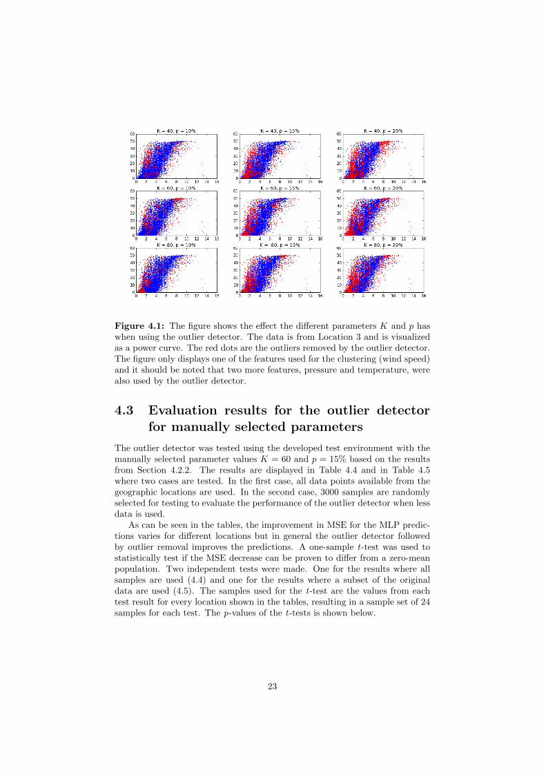
Figure 4.1: The figure shows the effect the different parameters K and p haswhen using the outlier detector. The data is from Location 3 and is visualizedas a power curve. The red dots are the outliers removed by the outlier detector.The figure only displays one of the features used for the clustering (wind speed)and it should be noted that two more features, pressure and temperature, werealso used by the outlier detector.

4.3 Evaluation results for the outlier detectorfor manually selected parameters

The outlier detector was tested using the developed test environment with themanually selected parameter values K = 60 and p = 15% based on the resultsfrom Section 4.2.2. The results are displayed in Table 4.4 and in Table 4.5where two cases are tested. In the first case, all data points available from thegeographic locations are used. In the second case, 3000 samples are randomlyselected for testing to evaluate the performance of the outlier detector when lessdata is used.

As can be seen in the tables, the improvement in MSE for the MLP predic-tions varies for different locations but in general the outlier detector followedby outlier removal improves the predictions. A one-sample t-test was used tostatistically test if the MSE decrease can be proven to differ from a zero-meanpopulation. Two independent tests were made. One for the results where allsamples are used (4.4) and one for the results where a subset of the originaldata are used (4.5). The samples used for the t-test are the values from eachtest result for every location shown in the tables, resulting in a sample set of 24samples for each test. The p-values of the t-tests is shown below.

23

Locations # samples Test 1 Test 2 Test 3 Test 4 Average ± σ

Location 1 6911 -0.47% 1.78% -0.50% -0.55% 0.07% ± 0.99%Location 2 7048 -0.81% 1.07% 2.45% 3.10% 1.45% ± 1.50%Location 3 7049 -0.24% 1.14% -0.35% 2.80% 0.84% ± 1.28%Location 4 6915 -0.08% -0.53% -0.83% 1.36% -0.02% ± 0.84%Location 5 7048 1.30% 3.00% 3.28% 1.52% 2.28% ± 0.87%Location 6 7049 0.77% 1.71% 1.62% 3.11% 1.8% ± 0.84%

Table 4.4: The table shows the MSE reduction in percentage when usingthe outlier detector compared to when not using it. The four tests is the testresults from the developed evaluation method. For each geographic location,every available data point were used and the number of samples is displayed inthe second column. In the final column, the average and the standard deviationof the four test results are displayed.

Locations Test 1 Test 2 Test 3 Test 4 Average ± σ

Location 1 -2.32% 0.15% -2.38% 0.77% -0.95% ± 1.42%Location 2 2.36% 2.44% 0.34% 1.98% 1.78% ± 0.85%Location 3 0.05% 4.35% 3.54% 1.9% 2.46% ± 1.65%Location 4 -0.39% 1.31% -0.36% -0.49% 0.02% ± 0.75%Location 5 1.93% 1.41% 3.38% -0.36% 1.59% ± 1.34%Location 6 1.76% 2.91% 2.53% 2.20% 2.35% ± 0.42%

Table 4.5: The table shows the same as in Table 4.4 except for in this case,instead of using every available sample, 3000 randomly selected samples fromeach location were used. This was done to test if the result would differ if afewer amount of data points were used.

• For the samples from Table 4.4 where all data points were used: pall =0.0011.

• For the samples from Table 4.5 where 3000 randomly sampled data pointswere used: p3000 = 0.0024.

This provides convincing evidence that the outlier detector has some effect onthe prediction results.

The data are plotted in Fig. 4.2 showing the power curves of the data beforeand after the outliers have been removed. The figure shows that the outlierdetector manages to mark the data points with low wind speed and high poweroutput and vice versa. The data becomes more shaped like a power curve, whichis reasonable since this relation between wind power production and wind speedis typical. It should be noted however, that the figures displays the targets (windpower production) and only one feature, wind speed, even though the outlieridentifier also used two more features: pressure and temperature. This explainswhy data points in the middle of the power curves sometimes are marked asoutliers since in relation to some other feature, they differ from the rest withintheir clusters.

24

(a) Location 1

(b) Location 2

(c) Location 3

(d) Location 4

(e) Location 5

(f) Location 6

Figure 4.2: Power curves before and after the identified outliers have beenremoved for the six different geographical locations. The left column shows theoriginal data, the middle shows the outliers marked in red and the right showsthe data when the outliers have been removed.

25

4.4 Testing the method for automatically select-ing the number of clusters, K

The method for selecting K was tested by comparing the test results betweenwhen the method was used to determine the value of K in the outlier detectorand when the parameter was manually selected, K = 60. The amount of datato be removed was set to p = 15% according to the test results in Section 4.2.2.The test was made on all the six geographical locations.

As can be seen in Table 4.6, the results indicate that the method did not seemto improve the predictions in comparison when K was manually selected since inmost of the cases, the MSE increased when using the method for automaticallyselecting K. Since so many test sets indicated worsened predictions, it wasdeemed unnecessary to further statistically test the results.

Locations # samples Test 1 Test 2 Test 3 Test 4 Average ± σ

Location 1 6911 0.90% -0.07% -2.17% -3.40% -1.18% ± 1.69%Location 2 7048 -1.91% -2.79% 0.71% -0.50% -1.12% ± 1.33%Location 3 7049 -1.00% 0.32% -4.10% -3.91% -2.17% ± 1.89%Location 4 6915 0.51% -0.02% 1.22% -0.73% 0.25% ± 0.71%Location 5 7048 0.77% -0.21% 1.29% -0.11% 0.44% ± 0.62%Location 6 7049 -1.68% -1.37% 0.67% -0.63% -0.75% ± 0.90%

Table 4.6: The table shows the MSE decreases in percentage for the outlierdetector when using the developed method for selecting K compared to whenmanually selecting the parameter value to K = 60. The four tests are the resultsfrom the different test data sets used in the developed evaluation method. Inthe final column the average and the standard deviation are displayed.

4.5 Testing the outlier stop criterion

A test was made for different values on ε using the evaluation method on onegeographic location, Location 6. The results are presented in Table 4.7. Ascan be seen, ε = 0.0014 gave the best performance and was used for testing theoutlier stop criterion method.

ε Test 1 Test 2 Test 3 Test 4 Average ± σ0.0006 0.5882 0.6014 0.6889 0.6152 0.6235 ± 0.03900.0010 0.5923 0.5858 0.5796 0.5886 0.5866 ± 0.00470.0014 0.5969 0.5819 0.5712 0.5859 0.5840 ± 0.00920.0018 0.5738 0.5961 0.5750 0.6044 0.5873 ± 0.01330.0022 0.5771 0.5871 0.5990 0.5968 0.5900 ± 0.0087

Table 4.7: The table shows the MSE of the four test sets of the evaluationmethod when testing on data from one location, Location 6, for different toler-ances, ε, on the stop criteria. It should be noted that these MSE values differfrom those in Table 4.3 since these tests were performed on a different location.

The outlier stop criterion method was tested the same way as the method

26

for selecting K, simply by first testing with the outlier stop criterion and thenwith manually setting p = 15%. The MSE decrease for each geographic locationand test set is shown in Table 4.8.

As can be seen in the table, the method does not seem to improve the resultsfor most of the cases compared to the case when p was manually set to 15%.The results seemed conclusive enough to conclude that no statistical testing ofthe results would be necessary to prove that the outlier stop criteria does notimprove the predictions.

Locations Test 1 Test 2 Test 3 Test 4 Average ± σd p d p d p d p

Location 1 -1.19% 20.8% -0.71% 12.8% 0.10% 16.2% -2.92% 15.7% -1.18% ± 1.10%Location 2 -2.67% 19.3% -0.24% 19.4% -2.16% 10.7% -1.24% 9.3% -1.58% ± 0.93%Location 3 0.32% 15.2% -0.48% 2.6% 0.02% 5.1% 0.12% 7.6% -0.01% ± 0.30%Location 4 1.82% 11.8% 2.39% 4.5% 1.29% 4.1% -0.19% 7.0% 1.33% ± 0.96%Location 5 -1.49% 3.1% -0.01% 11.5% -0.09% 3.2% 0.79% 10.2% -0.20% ± 0.82%Location 6 -2.54% 8.1% -0.94% 12.8% 1.07% 14.3% -1.78% 28.1% -1.05% ± 1.35%

Table 4.8: The table shows the MSE decrease in percentage when using theoutlier stop criterion to determine the amount of data to be removed, p inrespect to when manually setting the parameter to p = 15%. For each ofthe four tests the MSE decrease, d, in percentage is shown together with thevalue of p determined by the stop criterion. In the final column, the averageand standard variance deviation for the MSE decrease of the four test sets aredisplayed.

27

Chapter 5

Discussion & Conclusion

In this Master’s thesis a method for detecting outliers has been developed. Theproposed outlier detector uses unsupervised machine learning clustering to iden-tify anomalies in weather and wind power production data. The outlier detectorhas been tested using an advanced test environment developed to provide a re-liable test result based on the MSE of wind power predictions made by an MLPmodel. In addition, a feature ranking method has been developed to find rele-vant input features for the clustering as well as two parameter tuning techniquesfor automatically set the parameters: the number of clusters to be used and howmuch data is to be removed.

Data from six different geographical locations was used to test the perfor-mance of the outlier detector. The results provide evidence that the outlierdetector is able to reduce the MSE of predictions made by the MLP by remov-ing the data identified as outliers. However, none of the two parameter tunerswere proven to improve the results compared to the case when the parameterswere manually selected beforehand.

5.1 Machine learning methodology

5.1.1 Parameters

The outlier detector is proven to work properly when used on day-ahead windpower production prediction. However, many parameters were manually se-lected. Apart from the number of clusters and the amount of data to be removedfrom the original set, also the number of layers and number of hidden nodes inthe MLP where manually set to one and 20 respectively. According to StephenMarsland [18] the number of layers determine how complex functions is to bemodelled but more than two layers is rarely necessary. Marsland also claim thatthere is no obvious way to decide the number of hidden nodes and that one hasto simply try with different amounts and see how it effects the results.

The convergence for the Outlier stop criteria seen in Eq. (3.6) also has twoparameters that was not fully evaluated. These parameters are how many sam-ples to be used to measure convergence and what tolerance, ε, the criterionshould have. If these were properly analysed the Outlier stop criteria methodcould generate a better result. However, the observations made while testing

28

indicated that the result would not improve significantly enough to outperformthe case when the amount of data to remove, p, was manually selected.

5.1.2 Test environment

Developing a reliable test environment for testing machine learning predictionsusing big data requires a lot of consideration. Much time and effort were put intodeveloping a sound method for robust and reliable evaluation. Even though thetest environment is able to provide reliable proof there still exist an uncertaintyin the exact percentile improvement for the different location. Since the data isdivided randomly into test, validation and training the test will give inconsistentpercentile improvement for each location if run several times. What the testactually is consistent about is that the overall improvement is positive.

Further statistical testing should help to resolve the issue of the probabilisticuncertainty. However, due to the scarceness of the data this poses a problemfor further improvement of the statistical test results.

5.2 Comparison to previous research

This Master’s Thesis has contributed by providing new methodology within thefield of outlier detection within data used for wind power production prediction.There exists several methods for this purpose such as the ones developed byKusiak et al. [8] and Liu et al. [17]. However, there seem to be a lack of testresults and a limited amount of data used for testing. For instance, Kusiak etal. used a data set containing 3460 observations, while in this thesis data fromsix geographical locations each containing around 7000 observations were used.This can contribute to the scientific field since the test results from the differentlocations can show how the performance of a method can differ depending onthe data used.

The evaluation method used in this thesis can prove useful in further re-search. Much effort was put into making the evaluation method reliable. Inexisting papers, it seem to be common to separate a test set from the originaldata and use the rest for training a model and then solely rely on the modelsperformance on the test set. This method is mentioned by Marsland [18] andused by Kusiak et al. [8]. The method proposed in Section 3.5.2 does not onlyuse a subset of the original data for testing, but lets all data in turn act as bothtest and training data. This is a more effective way to make use of all dataavailable and provides a more reliable and accurate result.

5.3 Ethical review

The strongest ethical aspect of this Master’s thesis is that it contributes tomaking wind power a more predictable and therefore a more practical sourceof energy. It gets easier for electrical power producers and consumers to knowwhen to produce and when to consume energy depending on the energy prizes.

Another aspect is the fact that by identifying and removing outliers, thequality of existing data can increase and therefore limits the need for acquiringmore data which in some cases can be a costly and damaging process. The

29

method can also be used to clean data bases from unwanted data and there-fore free up digital storage space, limiting the need for ever increasing storagecapacity.

5.4 Future work

Since the two parameter tuners did not prove to increase the accuracy of thepredictions, there is still room for optimization of the outlier detector. Forinstance, another clustering method than K-means could be used. A methodwhich is able to select the number of clusters depending on the shape of the data.Fraley and Raftery [24] developed a methodology for this by using multivariateGaussian Mixture Models with Expectation Maximization and Bayesian modelselection. So using a similar approach instead of the K-means for clusteringcould result in a more optimal and general solution. This could work as long asthe method is able to settle for many clusters since it is of importance to dividethe data so that it properly divides the multivariate feature space and narrowsdown the spread of each feature within the clusters, making the clusters moretight.

The outlier detector was also unable to identify the data points where theenergy production was capped. This can be seen as an outlier behaviour forthe specific case of wind power production data. A method to identifies theseoutliers could be done by finding a way to identify a time series within the datawhere the wind power production is capped.

To further strengthen the evaluation of the method could be to test and see ifthe outlier detector can improve the result of another machine learning methodthan an ANN, such as an SVM. These algorithms have different methodologyand can therefore behave different when identified outliers are removed from thedata set.

30

Bibliography

[1] T. Ackermann, Wind power in power systems, vol. 140. Wiley OnlineLibrary, 2005.

[2] REN21, “Renewables 2016: Global status report,” REN21 Renewable En-ergy Policy Network/Worldwatch Institute, 2016.

[3] U. N. F. C. on Climate Change (UNFCCC), “Cop21 paris agreement.”

[4] P. Menanteau, D. Finon, and M.-L. Lamy, “Prices versus quantities: choos-ing policies for promoting the development of renewable energy,” Energypolicy, vol. 31, no. 8, pp. 799–812, 2003.

[5] C. Monteiro, R. Bessa, V. Miranda, A. Botterud, J. Wang, G. Conzelmann,et al., “Wind power forecasting: state-of-the-art 2009.,” tech. rep., ArgonneNational Laboratory (ANL), 2009.

[6] D. M. Hawkins, Identification of outliers, vol. 11. Springer, 1980.

[7] A. Ghoting, S. Parthasarathy, and M. E. Otey, “Fast mining of distance-based outliers in high-dimensional datasets,” Data Mining and KnowledgeDiscovery, vol. 16, no. 3, pp. 349–364, 2008.

[8] A. Kusiak, H. Zheng, and Z. Song, “Models for monitoring wind farmpower,” Renewable Energy, vol. 34, no. 3, pp. 583–590, 2009.

[9] E. Vladislavleva, T. Friedrich, F. Neumann, and M. Wagner, “Predictingthe energy output of wind farms based on weather data: Important vari-ables and their correlation,” Renewable energy, vol. 50, pp. 236–243, 2013.

[10] N. Amjady and F. Keynia, “Day-ahead price forecasting of electricity mar-kets by mutual information technique and cascaded neuro-evolutionary al-gorithm,” Power Systems, IEEE Transactions on, vol. 24, no. 1, pp. 306–318, 2009.

[11] N. Amjady, F. Keynia, and H. Zareipour, “Short-term wind power fore-casting using ridgelet neural network,” Electric Power Systems Research,vol. 81, no. 12, pp. 2099–2107, 2011.

[12] S. J. Kemp, P. Zaradic, and F. Hansen, “An approach for determiningrelative input parameter importance and significance in artificial neuralnetworks,” Ecological modelling, vol. 204, no. 3, pp. 326–334, 2007.

31

[13] A. Verikas and M. Bacauskiene, “Feature selection with neural networks,”Pattern Recognition Letters, vol. 23, no. 11, pp. 1323–1335, 2002.

[14] M. Gupta, J. Gao, C. C. Aggarwal, and J. Han, “Outlier detection fortemporal data: A survey,” IEEE Transactions on Knowledge and DataEngineering, vol. 26, pp. 2250–2267, Sept 2014.

[15] I. Ben-Gal, “Outlier detection,” in Data mining and knowledge discoveryhandbook, pp. 131–146, Springer, 2005.

[16] Y. Wan, E. Ela, and K. Orwig, “Development of an equivalent wind plantpower curve,” in Proc. WindPower, pp. 1–20, 2010.

[17] Z. Liu, W. Gao, Y.-H. Wan, and E. Muljadi, “Wind power plant predictionby using neural networks,” in 2012 IEEE Energy Conversion Congress andExposition (ECCE), pp. 3154–3160, IEEE, 2012.

[18] S. Marsland, Machine learning: an algorithmic perspective. CRC press,2015.

[19] J. MacQueen, “Some methods for classification and analysis of multivariateobservations,” in Proceedings of the Fifth Berkeley Symposium on Mathe-matical Statistics and Probability, Volume 1: Statistics, (Berkeley, Calif.),pp. 281–297, University of California Press, 1967.

[20] D. L. Davies and D. W. Bouldin, “A cluster separation measure,” IEEEtransactions on pattern analysis and machine intelligence, no. 2, pp. 224–227, 1979.

[21] J. C. Bezdek and N. R. Pal, “Some new indexes of cluster validity,” IEEETransactions on Systems, Man, and Cybernetics, Part B (Cybernetics),vol. 28, no. 3, pp. 301–315, 1998.

[22] H. Liu and L. Yu, “Toward integrating feature selection algorithms forclassification and clustering,” IEEE Transactions on knowledge and dataengineering, vol. 17, no. 4, pp. 491–502, 2005.

[23] K. Wagstaff, C. Cardie, S. Rogers, S. Schrodl, et al., “Constrained k-meansclustering with background knowledge,” in ICML, vol. 1, pp. 577–584, 2001.

[24] C. Fraley and A. E. Raftery, “How many clusters? which clusteringmethod? answers via model-based cluster analysis,” The computer journal,vol. 41, no. 8, pp. 578–588, 1998.

32

www.kth.se