Using the Wild Bootstrap to Quantify Uncertaintyin Diffusion Tensor Imaging

Brandon Whitcher,1* David S. Tuch,2,{ Jonathan J. Wisco,2

A. Gregory Sorensen,2 and Liqun Wang3

1Clinical Imaging Centre, GlaxoSmithKline, Hammersmith Hospital, London, United Kingdom2A. A. Martinos Center for Biomedical Imaging; Massachusetts General Hospital,

Charlestown, Massachusetts3Novartis Pharma AG, Basel, Switzerland

Abstract: Estimation of noise-induced variability in diffusion tensor imaging (DTI) is needed to objectivelyfollow disease progression in therapeutic monitoring and to provide consistent readouts of pathophysiol-ogy. The noise variability of nonlinear quantities of the diffusion tensor (e.g., fractional anisotropy, fiberorientation, etc.) have been quantified using the bootstrap, in which the data are resampled from the ex-perimental averages, yet this approach is only applicable to DTI scans that contain multiple averages fromthe same sampling direction. It has been shown that DTI acquisitions with a modest to large number ofdirections, in which each direction is only sampled once, outperform the multiple averages approach.These acquisitions resist the traditional (regular) bootstrap analysis though. In contrast to the regular boot-strap, the wild bootstrap method can be applied to such protocols in which there is only one observationper direction. Here, we compare and contrast the wild bootstrap with the regular bootstrap using MonteCarlo numerical simulations for a number of diffusion scenarios. The regular and wild bootstrap methodsare applied to human DTI data and empirical distributions are obtained for fractional anisotropy and thediffusion tensor eigensystem. Spatial maps of the estimated variability in the diffusion tensor principaleigenvector are provided. The wild bootstrap method can provide empirical distributions for tensor-derived quantities, such as fractional anisotropy and principal eigenvector direction, even when the exactdistributions are not easily derived. Hum Brain Mapp 29:346–362, 2008. VVC 2007 Wiley-Liss, Inc.

Key words: diffusion tensor imaging; bootstrap; confidence interval; fiber orientation; fractional anisot-ropy

INTRODUCTION

Regardless of the sampling scheme used, it is importantto properly characterize the amount of uncertainty in

derived quantities from the estimated diffusion tensor. Forquantities of interest based on linear combinations of ele-ments in the diffusion tensor, such as mean diffusivity,one can quantify variability through confidence intervals

Contract grant sponsor: NINDS; Contract grant number:NS046532; Contract grant sponsor: NCRR; Contract grant number:RR014075; Contract grant sponsor: NCI; Contract grant number:5T32CA09502; Contract grant sponsor: NIBIB ; Contract grantnumbers: U54EB005149; Contract grant sponsors: GlaxoSmithKline,Athinoula A. Martinos Foundation, Mental Illness and Neuro-science Discovery (MIND) Institute, National Alliance for MedicalImage Computing (NAMIC).

*Correspondence to: Brandon Whitcher, Clinical Imaging Centre,GlaxoSmithKline, Hammersmith Hospital, Du Cane Road, LondonW12 0NN United Kingdom. E-mail: brandon.j.whitcher@gsk.com{Present address: Novartis Pharma AG, Basel, Switzerland.Received for publication 9 November 2005; Revised 30 November2006; Accepted 20 February 2007

DOI: 10.1002/hbm.20395Published online 23 April 2007 in Wiley InterScience (www.interscience.wiley.com).

VVC 2007 Wiley-Liss, Inc.

r Human Brain Mapping 29:346–362 (2008) r

derived from the noise properties of magnitude imagesand the theory of linear models [Salvador et al., 2005].However, quantities based on nonlinear combinations ofelements from the diffusion tensor (e.g., eigenvalues,eigenvectors, fractional anisotropy, etc.) are not easilyobtained analytically1 and computational methods are uti-lized instead. When a relatively low number of gradientdirections are sampled, it is common to obtain multiplemeasurements in each direction during the scanning ses-sion. If this is the case, then the bootstrap [Efron, 1981;Efron and Tibshirani, 1993] has been used to help quantifyuncertainty in scalar summaries of DTI [Heim et al., 2004;Jones, 2003; Pajevic and Basser, 2003]. Uncertainty in thediffusion tensor is also very important for tractography[Behrens et al., 2003] and the bootstrap has already beensuccessfully applied [Jones and Pierpaoli, 2005; Jones et al.,2005].The bootstrap method, as previously implemented in

DTI, requires multiple observations per gradient directionin order to perform the resampling. With samplingschemes acquiring a large number of directions being usedmore and more in a clinical setting [Jones, 2004; Joneset al., 1999a], it is becoming less likely that more than onemeasurement per gradient direction is obtained—exclud-ing the application of this particular implementation of thebootstrap (we call this the regular bootstrap from now on).An investigation into how many repeat acquisitions arerequired to gain accurate results from the regular boot-strap concluded that no benefit in accuracy or precisionwas gained by using more than seven repeat acquisitionsand fewer than four repeat acquisitions resulted in poorprecision with significant errors [O’Gorman and Jones,2005]. For example, with a whole-brain acquisition proto-col taking 10–15 min to acquire a single volume, it wouldbe difficult to push the number of repeat acquisitions toler-ated by patients with mild disorders beyond three or four.Being able to apply resampling procedures to either (a)fewer repeat acquisitions or (b) acquisitions with a rela-tively high number of gradient directions with no repeatedmeasurements without losing the ability to characterize theintrinsic variability of statistical summaries of DTI ishighly desirable.We introduce model-based resampling techniques

[Davison and Hinkley, 1997], in particular, the wild boot-strap [Flachaire, 2005; Liu, 1988], that may be applied tothe residuals from the multiple linear regression modelused to estimate elements of the diffusion tensor at eachvoxel. The wild bootstrap is specifically designed to workwhen the model is heteroscedastic; that is, when the var-iance of the errors is not constant for all observations. Inthe case of DTI, this corresponds to the assumption of non-constant variance for the log-transformed NMR signal[Basser et al., 1994; Salvador et al., 2005]. The relationship

between noise and b-value and their influence on quanti-ties derived from the diffusion tensor, such as fractionalanisotropy, was recently described in Jones and Basser[2004]. A simple modification to the basic model-basedbootstrap allows this methodology to be applied whenmultiple measurements are acquired in each gradientdirection. Thus, the model-based bootstrap techniques pre-sented here may be applied to both research and clinicalDTI protocols assuming that more than six gradient direc-tions have been acquired or that a six-direction gradientencoding scheme has been acquired more than once.Statistical methods, such as the bootstrap, are not the

only way to quantify uncertainty in DTI. There are numer-ous references based on analytical techniques, such as‘‘propagation of errors’’. First and second-order correctionsto the eigenvalues and eigenvectors from perturbationtheory were used to correct for noise distortions in Ander-son [2001]. Measures of anisotropy, obtained without diag-onalizing the tensor, were studied using propagation oferrors to compare sampling schemes in Poonawalla andZhou [2004]. Numerical methods, such as Monte Carlosimulation, have also been used to investigate the effect ofnoise on quantitative measurements of anisotropy espe-cially those based on eigenvalues (i.e., the sorting bias)[Batchelor et al., 2003; Pierpaoli and Basser, 1996; Skareet al., 2000].This study investigates the ability of model-based resam-

pling, in particular, the wild bootstrap, to provide reasona-ble estimates of variability for derived quantities of the dif-fusion tensor when one or more measurements per gradi-ent direction are available. Two sampling schemes, sixdirections and 60 directions, are used to produce bothsimulated and clinical DTI data. Comparisons are madefor regular and wild bootstrap estimates of variability onthe eigenvalues, fractional anisotropy, and fiber orientationderived from the diffusion tensor. With standard errorsbased on the bootstrap now available for all image acquisi-tion schemes, it is hoped that reporting both parameterestimates and standard errors for summaries of anisotropywill become more widespread.

THEORY

The regular bootstrap is a general statistical techniquewhere an observed set of measurements is sampled withreplacement over-and-over again in order to characterize astatistic of interest [Davison and Hinkley, 1997; Efron andTibshirani, 1993]. The regular bootstrap places equal prob-ability on independent observations when resampling, andis therefore only appropriate when more than one mea-surement per direction is available (although this is notstrictly true, a point which we move onto later). Thisframework is common in DTI scans when the acquisitionsequence contains relatively few gradient directions (e.g.,six) but becomes less clinically feasible as the number ofgradient directions increases. Further details and examples

1 We assume that the diffusion tensor contains non-zero off diago-nal elements.

r The Wild Bootstrap in DTI r

r 347 r

concerning the implementation of the regular bootstrap inDTI data analysis may be found in Pajevic and Basser[2003] and Heim et al. [2004].Although six gradient directions are the minimum num-

ber to estimate the unique elements of the diffusion tensor,there are numerous sampling schemes that have been rec-ommended with many more gradient directions [Batcheloret al., 2003; Hasan and Narayana, 2003; Jones et al., 1999a,b] or it is common practice to obtain several measurementsin each direction when a relatively low number of gradientdirections are sampled. Because of the constraints in a clin-ical setting there are relatively few DTI scans with a largenumber of directions and repeated measurements. Hence,obtaining estimates of standard errors for scalar quantitiesof interest based on the diffusion tensor are not availableusing the regular bootstrap. This leads us to consider alter-native bootstrap methodology that operates within the log-linear relationship between echo attenuation and the diffu-sion model.

Model-Based Resampling: Homoscedastic Errors

First, we describe the theory around the model-basedresampling of errors in a linear regression model and thenintroduce the wild bootstrap. Model-based resampling inlinear regression is a popular nonparametric technique toinfer properties of the parameter estimates from the linearmodel. Let us assume that the standard model for signalintensity in DTI is given by SðxiÞ ¼ S0 exp �bxTi Dxi

� �,

where D is the diffusion tensor, xi ¼ (xi1, xi2, xi3)T is the

gradient direction for the ith observation (i ¼ 1,. . .,N) andb is the diffusion weighting. Applying the log transform toboth sides allows us to use notation for a multiple linearregression model [Basser et al., 1994]

y ¼ Xdþ e; ð1Þ

to estimate the diffusion tensor from observed data. InEq. (1) y is a length N vector of the log-transformed signalintensities, X is a N � 7 direction matrix

�bx211 �bx212 �bx213 �2bx11x12 �2bx11x13 �2bx11x13 1�bx221 �bx222 �bx223 �2bx21x22 �2bx21x23 �2bx22x23 1

..

. ... ..

. ... ..

. ... ..

.

�bx2N1 �bx2N2 �bx2N3 �2bxN1xN2 �2bxN1xN3 �2bxN2xN3 1

26664

37775

ð2Þ

d ¼ [Dxx Dyy Dzz Dxy Dxz Dyz log(S0)]T and e is a length N

vector of errors. The ordinary least-squares (OLS) estimateof d is given by d¼ðXTXÞ�1XTy. After the initial OLSoperation, a weighting matrix W may be calculated via

W¼ IN expðXdÞ; ð3Þ

where IN is the N � N identity matrix. The weightedleast-squares (WLS) estimate of d is then given by

d¼ðXTW�2XÞ�1XTW�2y [Salvador et al., 2005]. This imple-mentation of WLS is similar to the approach found inBasser et al. [1994], the difference being that fitted valuesfrom the least-squares regression are used instead of theobservations in constructing the weighting matrix W.The assumptions we make on the structure of e determine

which bootstrap method is appropriate. Under the assump-tion that e is a vector of independent and identically distrib-uted (IID) random variables with zero mean, the linearregression would be termed homoscedastic and we would beable to randomly sample with replacement from the errors.Model-based resampling of the errors would take the form

y?i ¼ ðXdÞi þ e?i ; i ¼ 1; . . . ;N; ð4Þ

where (Xd)i is the product of the ith row of X and d, and e?iis a random sample from the residuals of the original regres-sion model. Performing WLS on y$ will produce a model-based bootstrap estimate of the tensor d$. Repeating thesesteps, resampling and estimation, builds up a collection oftensors called a (model-based) bootstrap distribution. Sum-mary statistics from this empirical distribution can be usedto describe the original parameter estimate.

Model-Based Resampling: Heteroscedastic Errors

The assumption of homoscedasticity is not valid for DTIwhen a linear regression model is used to estimate the dif-fusion tensor. This violation is induced by applying thelogarithmic transform in order to achieve the linear rela-tionship in Eq. (1) and is overcome through the use ofWLS regression, as originally noted in Basser et al. [1994].When the assumption of IID errors is not valid, the regres-sion model is termed heteroscedastic. When a relativelysmall number of gradient directions are used to acquirethe data, a simple modification to the basic model-basedbootstrap procedure can adapt to the situation where mul-tiple measurements per direction are available. We callthis technique ‘‘resampling within gradient directions’’(RWGD). Rewrite the vector of observations (log-trans-formed signal intensities) as being indexed by gradientdirections and measurements per direction

y ¼ ½y0;1 y0;2 � � � y0;m y1;1 y1;2 � � � y1;m � � � y6;1 y6;2 � � � y6;m�T

¼ ½y0 y1 � � � y6�T; ð5Þ

in this specific case y0 denotes the b ¼ 0 acquisitions andy1,. . .,y6 denote the acquisitions corresponding to six gradi-ent directions. For convenience, assume that the rows of Xmay be indexed the same way. The RWGD bootstrap sam-ple would take the form

y?j;k ¼ ðXdÞj;k þ e?k ; j ¼ 0; 1; . . . ; 6; k ¼ 1; . . . ;m; ð6Þ

so that each subvector yj conforms with Eq. (4), thusensuring that all resampling is kept within each gradientdirection.

r Whitcher et al. r

r 348 r

The wild bootstrap [Liu, 1988] is a method for model-based resampling in heteroscedastic linear regression withan unknown form; i.e., when the errors have an arbitraryvariance structure. Model-based resampling, using thewild bootstrap, is given by

y?i ¼ ðXdÞi þ aiuie?i ; i ¼ 1; . . . ;N; ð7Þ

where ai is a weight in order to produce a heteroscedastic-ity consistent covariance matrix estimator (HCCME), ui isthe residual and e?i is drawn from the distribution F. TheHCCME is required because a standard assumption of lin-ear regression models—the error terms have a constantvariance—is violated here [MacKinnon and White, 1985].Instead of resampling from the residuals of the linearregression, only valid in the homoscedastic case, the wildbootstrap samples from an auxiliary distribution F andmultiplies this random variable with a rescaled version ofthe residual aiui using a local estimate of the covariancematrix. Examples of such HCCMEs include

ai ¼ffiffiffiffiffiffiffiffiffiffiffin

n� p

r; ai ¼

ffiffiffiffiffiffiffiffiffiffiffiffi1

1� hi

r; ai ¼ 1

1� hi; ð8Þ

where n is the total number of observations, p is the num-ber of estimated parameters, and hi is the ith diagonal ele-ment from H¼X(XTX)�1 XT, the so-called hat matrix fromOLS regression. Detailed explanations of the HCCMEs arebeyond the scope of this study and can be found in MacK-innon and White [1985]. Briefly, the first form in Eq. (8)comes from a degrees of freedom correction and the sec-ond and third forms can be derived from jackknife-basedestimators of the covariance matrix. The bootstrap per-formance between the different versions is discussed inFlachaire [2005] and results from DTI-specific simulationsare provided in this article.The random variable e$ obtained from the auxiliary dis-

tribution must satisfy

Eðe?Þ ¼ 0; ð9Þ

Eðe?2Þ ¼ 1; ð10Þ

that is, its first moment is zero and its second moment isone, to ensure that the residual from the wild bootstrap inEq. (7) retains the same first and second moments as thetrue residual. An additional condition

Eðe?3Þ ¼ 1; ð11Þ

its third moment is one, is commonly added to help definethis distribution. It has been shown, assuming Eqs. (9)–(11), that the first three moments of the bootstrap distribu-tion of an HCCME-based test statistic agree with thosefrom the true distribution of the statistic up to order n�1

[Liu, 1988]. Two suggestions for the auxiliary distributionF are

F1: e?i ¼ �ð ffiffiffi5

p �1Þ=2 with probability p¼ð ffiffiffi5

p �1Þ=ð2 ffiffiffi5

p Þ,ð ffiffiffi

5p þ1Þ=2 with probability 1�p;

�

ð12Þ

[Mammen, 1993] and the Rademacher distribution

F2 : e?i ¼1 with probability 0.5,�1 with probability 0.5;

�ð13Þ

[Davidson and Flachaire, 2001; Liu, 1988]. Simulation stud-ies in Davidson and Flachaire [2001] have indicated thatthe wild bootstrap using F2 outperforms the wild bootstrapusing F1, especially when the errors follow a skewed dis-tribution. Additional proposals for auxiliary distributionsmay be found in Liu [1988] and Mammen [1993].Note the residuals are no longer resampled in Eq. (7) to

generate the wild bootstrap sample, unlike the ordinarymodel-based bootstrap sample in Eq. (4). This respects theheteroscedasticity in the model but still produces enoughvariability to draw inference about the parameters (diffu-sion tensor elements) in the multiple linear regressionmodel. An example of the wild bootstrap applied to a sin-gle voxel, taken from Whitcher et al. [2005], is provided inFigure 1. The original voxel was chosen because it deviatesfrom isotropy (FA ¼ 0.85). The fit from the multiple linearregression model is provided along with the individualmeasurements. The residuals ui are then calculated andmodified via aiuie?i , where ai ¼ (1 – hi)

�1/2, to produce thewild bootstrap residuals. The wild bootstrap residuals arethen added back to the fitted model to produce a newmodel-based resampling of the data. Estimating the diffu-sion tensor via multiple linear regression produces a newfit from which scalar summaries may be derived (e.g., FA¼ 0.9). Performing this operation a number of times gener-ates a wild bootstrap distribution for the parameter of in-terest, in this case FA.

MATERIALS AND METHODS

Simulation of DTI Data

Signal intensities, assumed to be taken from magnitudeimages, for single voxels were simulated using two sourcesof uncertainty. Euler angles of the principal eigenvectorwere drawn from a normal (Gaussian) distribution withmean m ¼ 458 and variance s2 ¼ 98. Measurement errorwas drawn from the Rician distribution for each gradientdirection with a signal-to-noise ratio of SNR [ {5,10,20} forthe b ¼ 0 images. Sampling from the Rician distribution isrelatively straightforward, computationally, because of itsrelationship to the noncentral w2 distribution with twodegrees of freedom and the fact that random number gen-erators for the noncentral w2 distribution are widely avail-able. Three sets of simulations were performed, one foreach type of tensor: prolate (l1, l2, l3) ¼ (1.5, 0.4, 0.4)mm2/ms, oblate (l1, l2, l3) ¼ (0.9, 0.8, 0.6) mm2/ms, and

r The Wild Bootstrap in DTI r

r 349 r

isotropic (l1, l2, l3) ¼ (0.767, 0.767, 0.767) mm2/ms. Alltensor models have the same trace, Si li ¼ 2.3 mm2/ms,and are based on previously reported normal values[Pierpaoli et al., 1996].The first stage of the simulation procedure produced

1,000 Monte Carlo simulations in order to obtain sufficient‘‘ground truth’’ for comparison with the proposed boot-strap techniques. A single realization from the MonteCarlo sample was drawn at random and 999 bootstrapiterations were computed based on that realization. Sum-mary statistics, based on the eigenvalues (or functions ofthem) and eigenvectors, were computed for each set ofMC and bootstrap realizations. This first stage was per-formed 250 times to provide a measure of uncertainty inthe MC and bootstrap procedures. Thus, a total of 1,000 �250 ¼ 250,000 iterations were run and summaries of thesimulation-based results involve 250 values for each statis-tic of interest.Two simulation scenarios were considered (all with b ¼

700 s/mm2 unless otherwise specified): one with a modest

number of acquisitions, 14 in total, either two b ¼ 0 and 12diffusion-weighted with six gradient directions (NEX ¼10) or two b ¼ 0 and 12 diffusion-weighted with 12 gradi-ent directions [Jones et al., 1999b]; and one with a rela-tively large number of acquisitions, 70 in total, either 10 b¼ 0 and 60 diffusion-weighted with six gradient directions(NEX ¼ 10) or 10 b ¼ 0 and 60 diffusion-weighted with 60gradient directions. When implementing the regular boot-strap on the 6-direction data (NEX ¼ 10), each regularbootstrap realization produced 70 diffusion-weightedimages (10 T2 + 60 diffusion-weighted) drawn withreplacement from the original 70 images. Similarly, whenNEX ¼ 2 each regular bootstrap realization produced 14diffusion-weighted images (2 T2 + 12 diffusion-weighted)drawn with replacement from the original 14 images.The sampling scheme proposed in this article is equiva-

lent to the specific case of ri ¼ ni, for all i, using the nota-tion from Pajevic and Basser [2003] and correspondsexactly with the bootstrap method provided in Heim et al.[2004]. When implementing the wild bootstrap on the 60-

Figure 1.

Graphical illustration of the wild bootstrap on a single voxel where b ¼ 0 for indices 1–10 and

b ¼ 700 s/mm2 for indices 11–70; (a) observations and fitted values from the diffusion tensor,

(b) original and bootstrap residuals from the model fit, (c) bootstrap observations with new fit-

ted values, and (d) bootstrap distribution of fractional anisotropy. [Color figure can be viewed

in the online issue, which is available at www.interscience.wiley.com.]

r Whitcher et al. r

r 350 r

direction data, the two-point distribution F2 was usedexclusively to generate e; the heteroscedasticity consistentcovariance matrix estimator used was a ¼ 1=

ffiffiffiffiffiffiffiffiffiffiffiffi1� h

pwhere

h is the diagonal element vector from the hat matrix) andu ¼ y� Xd defined the residual vector.

Human MR Imaging

Data were acquired from one normal subject (28-year-old male Caucasian) in a Siemens Allegra 3.0 Tesla scan-ner using a single channel head coil. The data were col-lected using a protocol approved by the MassachusettsGeneral Hospital Internal Review Board. The participantprovided informed consent in writing prior to the scansession. Two sets of images were obtained: the firstconsisted of 10 measurements of six gradient directions(b ¼ 700 s/mm2) and 10 T2 images (b ¼ 0) and the secondconsisted of a single measurement of 60 gradient direc-tions (b ¼ 700 s/mm2) and 10 T2 images (b ¼ 0). For bothscans, however, the slice prescription was identical: 64 sli-ces acquired in the AC-PC plane, TR/TE ¼ 7,900/83 ms,gmax ¼ 31 mT/m, FoV ¼ 256 � 256, base resolution ¼ 128� 128, 8.0 mm3 isotropic voxels. Acquisition time for eachscan was 9:21. The specific choices required to implementthe wild bootstrap were identical to the simulated DTIdata. Note that cardiac gating was not used in the acquisi-tion protocol.

Computational Details

To clarify notation and terminology, we use the termmultiple linear regression model to denote Eq. (1). Wereserve the term ‘‘multivariate’’ for the model below. Put-ting aside, for the moment, the resampling of residualshere we focus on estimating the diffusion tensor for a largenumber of voxels. There are clear advantages in the com-putational efficiency of DTI data analysis over a slice, orindeed the whole volume, when one formulates the modelin Eq. (1) for all voxels as a multivariate multiple linearregression

Y ¼ X�þ e; ð14Þ

where Y is a N � V response matrix with each column rep-resenting the log-transformed signal intensity from a differ-ent voxel, D is a 7 � V matrix with each column being thediffusion tensor estimates, along with the b ¼ 0 term. Theadvantage of organizing the data in this way facilitates asingle application of linear algebra techniques, such as theQR or singular-value decomposition, to estimate the diffu-sion tensors for all voxels simultaneously. This eliminatesthe need to loop over the voxels in order to perform a singlemultiple linear regression and produces much more effi-cient algorithms in common data analysis packages (suchas Matlab or R) where loops, especially nested loops, areslow.

RESULTS

Simulated DTI Data

Figures 2–4 show boxplots2 of the simulation study com-paring MC simulations with regular and wild bootstraprealizations for the 6-direction data (NEX ¼ 10) and 60-direction data (NEX ¼ 1) for SNR & 20. Horizontal linesindicate the true value when available. The figures shownhere utilize the second choice of HCCME from Eq. (8); i.e.,ai ¼ (1–hi)

�1/2. Simulations were performed using all threeHCCMEs with no substantial difference between the char-acteristics of the eigenvalues or FA.For the prolate tensor, averages for l2 and l3 exhibit a

small amount of bias due to sorting while l1 is much lessaffected [Pierpaoli and Basser, 1996]. Both regular andwild bootstrap estimates of the average show much morevariability, but this is to be expected since they are basedon a single observation, whereas the MC averages have1,000 observations. Standard deviations of the eigenvaluesindicate a difference in sampling schemes, although notenough to be clinically meaningful. The regular bootstrapestimates of the eigenvalue SD are negatively biased forthe 6-direction scheme and are much more variable thanthe wild bootstrap results for the 60-direction scheme,even though the former has 10 measurements per gradientdirection. This may be due purely to the number of direc-tions sampled, not the bootstrap methodology, with the60-direction scheme producing more stable estimates ofthe diffusion tensor elements from which these eigenval-ues are based; as noted previously by Jones [2004].One potential source of variability comes from the fact

that the regular and wild bootstrap procedures wereapplied to separate data sets. An additional step wasincluded where the wild bootstrap was applied to the datafrom the 6-direction scheme without altering the algo-rithm. No difference in performance, as measured by esti-mates of the average and SD of the eigenvalues, wasdetected when the wild bootstrap was applied to the datafrom the 6-direction scheme compared to the regular boot-strap procedure.Average fractional anisotropy (FA) is accurately esti-

mated by the wild bootstrap for 60-direction data withincreased precision when compared with the regular boot-strap for the 6-direction data (the true value of FA is�0.69). The SD of estimated FA values is less for the 60-direction scheme and its bootstrap estimate of SD appearsto be much less biased than the results from the regularbootstrap on the 6-direction scheme. When looking at theso-called cone of uncertainty [Jones, 2003], neither boot-strap technique adequately estimates the 95 percentile

2 The box portion of each boxplot element captures the interquar-tile range (25% to 75%) of the observations and the line roughly inthe middle corresponds to the median of the observations. Obser-vations beyond 1.5 times the interquartile range, in either direc-tion, are drawn as individual points.

r 351 r

r The Wild Bootstrap in DTI r

Figure 2.

Summary statistics derived from 250 iterations of the simulation

study using a prolate tensor (l1, l2, l3) ¼ (1.5, 0.4, 0.4) mm2/ms,

FA & 0.69, SNR ¼ 20. The average and standard deviation (SD)

were computed for all three eigenvalues, fractional anisotropy, and

the 95 percentile in the minimum angle subtended, under both ac-

quisition schemes (6- and 60-directions) and the three methods

(Monte Carlo simulation, regular bootstrap, and wild bootstrap).

The labels correspond to, from left to right, 6-directions (NEX ¼10) using MC simulation, 6-directions (NEX ¼ 10) using the regu-

lar bootstrap, 60-directions using MC simulation, and 60-directions

using the wild bootstrap. [Color figure can be viewed in the online

issue, which is available at www.interscience.wiley.com.]

r 352 r

r Whitcher et al. r

from the MC simulations. Instead, both techniques are atleast 28 less (20%) when comparing median values (solidbar in the boxplot) with the MC simulation results. Such

discrepancies, between the MC simulations and bootstrapsamples, are not apparent in the other univariate summa-ries of the diffusion tensor model displayed but those

Figure 3.

Summary statistics derived from 250 iterations of the simulation

study using an oblate tensor (l1, l2, l3) ¼ (0.9, 0.8, 0.6) mm2/

ms, FA & 0.20, SNR ¼ 20. The average and standard deviation

(SD) were computed for all three eigenvalues, fractional anisot-

ropy, and the 95 percentile in the minimum angle subtended,

under both acquisition schemes (6- and 60-directions) and the

three methods (Monte Carlo simulation, regular bootstrap, and

wild bootstrap). The labels are identical to those in Figure 2.

[Color figure can be viewed in the online issue, which is available

at www.interscience.wiley.com.]

r 353 r

r The Wild Bootstrap in DTI r

quantities are inherently more stable; e.g., the mean andstandard deviation. Given that the bootstrap estimates ofthe 95 percentile are based on a single realization of the

prolate tensor model, instead of 1,000 realizations, there isnot enough information to accurately reproduce more diffi-cult quantities such as extreme values.

Figure 4.

Summary statistics derived from 250 iterations of the simulation

study using an isotropic tensor (l1, l2, l3) ¼ (0.767, 0.767,

0.767) mm2/ms, SNR ¼ 20. The average and standard deviation

(SD) were computed for all three eigenvalues, fractional anisot-

ropy, and the 95 percentile in the minimum angle subtended,

under both acquisition schemes (6- and 60-directions) and the

three methods (Monte Carlo simulation, regular bootstrap, and

wild bootstrap). The labels are identical to those in Figure 2.

[Color figure can be viewed in the online issue, which is available

at www.interscience.wiley.com.]

r 354 r

r Whitcher et al. r

The oblate tensor in Figure 3 shows the usual sortingbias in the average for all three eigenvectors by both boot-strap methods, with similar precision but slightly morebias in l1 and l3 for the wild bootstrap. The regular boot-strap for the 6-direction data and the wild bootstrap forthe 60-direction data produced similar quality estimates ofeigenvalue SD for all three eigenvalues, with a slight nega-tive bias in the regular bootstrap. This is likely due to thenumber directions in the encoding scheme and not specifi-cally attributable to the bootstrap methodology. AverageFA shows a slight positive bias for both sampling schemes,with the wild bootstrap on the 60-direction data being lessprecise when compared with the regular bootstrap appliedto the 6-direction data. The SD of estimated FA showsonly minor differences between the two bootstrap proce-dures, with a slight negative bias for the wild bootstrap.Estimates of angular difference for the cone of uncertaintyare much improved versus the prolate tensor. Both boot-strap methods demonstrate a negative bias when estimat-ing the 95 percentile of the minimum angle subtended;this is similar to the case of the prolate tensor and is mostlikely due to the difficulties in estimating extremes fromthe bootstrap applied to a single realization.The isotropic tensor in Figure 4 exhibits pronounced

effects from sorting bias in the eigenvalues. Both bootstraptechniques suffer from increased bias, positive for l1 andnegative for l3, when compared with the MC simulations.When comparing estimates of the SD for each eigenvalue,the 60-direction scheme exhibits a larger SD, both in simu-lation and through the wild bootstrap, but the positivebias from the wild bootstrap does not appear to be muchlarger than the positive bias present in the regular boot-strap for the 6-direction data. The true FA for all simula-tions is zero, but with the inclusion of Rician noise this isnot possible to attain and thus positive bias in estimates ofFA (whether from MC or bootstrap realizations) is to beexpected. Bias from the true value of zero is around 0.08for the MC simulations, a little less for the 6-directionscheme, and the bootstrap realizations exhibit positive biasabove and beyond that to be expected from the MC results(on the order of 0.02–0.04 units FA). The estimated SD ofFA was very similar for the two sampling schemes for theMC simulations, with a slight positive bias when applyingthe bootstrap techniques. The wild bootstrap does exhibitincreased bias when compared with the regular bootstrap.This is most likely due to the encoding scheme and notthe bootstrap methodology. With 10 acquisitions under thesix-direction scheme, there is more information about thevariability of the data instead of a single acquisition with60 directions. Thus, the wild bootstrap, based on the 60-direction data, is exhibiting increased variability when esti-mating FA. The 95 percentile of the angular difference isvery close to 90 degrees, with a small negative bias for thebootstrap techniques and a large left-hand tail in theobserved distribution of angles.When the SNR was reduced to 5 or 10, the performances

of the regular and wild bootstrap methods, relative to their

MC simulations, follow the patterns observed in Figures2–4 with a few notable differences (not shown). For theprolate tensor, decreased SNR induces substantial negativebias in the estimated major eigenvalue when using onlysix directions, and thus, negative bias in FA. This is notobserved in estimates obtained from the 60-direction data.The ability of either bootstrap method to accurately repro-duce the uncertainty in the angular difference is much bet-ter; a negligible bias is observed when compared withhigh SNR. Patterns in the performance of either bootstrapmethod did not appear to be differentially affected bydecreasing SNR for the oblate and isotropic tensors.

Human DTI Data

Statistical summaries of fractional anisotropy (FA) colormap and bootstrap standard error (SE), in grayscale, foraxial slices through the centrum semiovale (Fig. 5, panelsa–e, a‘�e’; k–o, k‘�o’) and through the caudal midbrain/rostral pons (Fig. 5, panels f–j, f‘�j’; p–t, p‘�t’) are dis-played for both the 6- and 60-direction data. Minor differ-ences between the two sampling schemes for the estimatedFA, colored by the direction of the principal eigenvector[Pajevic and Pierpaoli, 1999], are apparent.From motor cortex, the corticospinal tracts travel inferi-

orly through

1. centrum semiovale in the cerebral hemispheres,2. posterior limb of the internal capsule,3. cerebral peduncles of the midbrain, and4. pons before reaching the medulla to form the pyra-

mids.

The axial views in Figure 5 demonstrate the corticospi-nal tracts in the cerebral hemispheres and brainstem.Although the corticospinal tracts are well defined in the cer-ebral peduncles, they are not as well defined in the areas ofthe centrum semiovale and pons where other white mattertracts intersect. To illustrate, the FA color map shows thecentrum semiovale as a mostly ‘‘blue’’ structure (oriented inthe superior-inferior direction) in superior slices, but inter-secting ‘‘red’’ fibers (oriented left-right) can be seen in infe-rior slices (Fig. 5, panels a–e, white arrows). Arrows areonly shown on every other slice and in the six-directiondata only for simplicity. A similar trend is shown in thetransition from the caudal midbrain to the rostral pons (Fig.5, panels f–j). Thus, we expected that lower bootstrap SEwould be found in voxels corresponding to the corticospinaltracts of the cerebral peduncles as compared to either thecentrum semiovale or rostral pons in both the 6- and 60-direction data. Figure 5, panels a‘�e’ and f’�g’ show thatthis is indeed the case, although the results are more appa-rent in the brainstem. Figure 6, a map of the bootstrap SEfor the principal eigenvector Euler angle, accentuates theresults from SE maps in Figure 5 and emphasizes the resultsthat angular uncertainty is low in regions where the whitematter bundles are uniform in direction and high in regions

r The Wild Bootstrap in DTI r

r 355 r

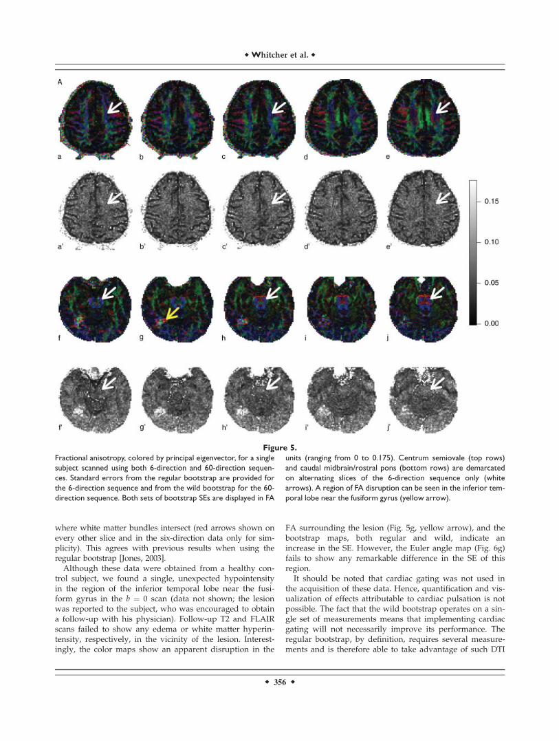
where white matter bundles intersect (red arrows shown onevery other slice and in the six-direction data only for sim-plicity). This agrees with previous results when using theregular bootstrap [Jones, 2003].Although these data were obtained from a healthy con-

trol subject, we found a single, unexpected hypointensityin the region of the inferior temporal lobe near the fusi-form gyrus in the b ¼ 0 scan (data not shown; the lesionwas reported to the subject, who was encouraged to obtaina follow-up with his physician). Follow-up T2 and FLAIRscans failed to show any edema or white matter hyperin-tensity, respectively, in the vicinity of the lesion. Interest-ingly, the color maps show an apparent disruption in the

FA surrounding the lesion (Fig. 5g, yellow arrow), and thebootstrap maps, both regular and wild, indicate anincrease in the SE. However, the Euler angle map (Fig. 6g)fails to show any remarkable difference in the SE of thisregion.It should be noted that cardiac gating was not used in

the acquisition of these data. Hence, quantification and vis-ualization of effects attributable to cardiac pulsation is notpossible. The fact that the wild bootstrap operates on a sin-gle set of measurements means that implementing cardiacgating will not necessarily improve its performance. Theregular bootstrap, by definition, requires several measure-ments and is therefore able to take advantage of such DTI

Figure 5.

Fractional anisotropy, colored by principal eigenvector, for a single

subject scanned using both 6-direction and 60-direction sequen-

ces. Standard errors from the regular bootstrap are provided for

the 6-direction sequence and from the wild bootstrap for the 60-

direction sequence. Both sets of bootstrap SEs are displayed in FA

units (ranging from 0 to 0.175). Centrum semiovale (top rows)

and caudal midbrain/rostral pons (bottom rows) are demarcated

on alternating slices of the 6-direction sequence only (white

arrows). A region of FA disruption can be seen in the inferior tem-

poral lobe near the fusiform gyrus (yellow arrow).

r Whitcher et al. r

r 356 r

acquisition schemes. One procedure is not necessarily opti-mal for all situations and caution should be exercisedwhen deciding on the specific DTI acquisition scheme, notonly for data quality implications but also its impact ondata modeling and analysis.

DISCUSSION AND CONCLUSIONS

A collection of resampling techniques has been pro-posed, which provides estimates of uncertainty in univari-ate summaries of the estimated diffusion tensor, regardlessof the specific DTI acquisition method assuming that morethan six gradient directions have been acquired or a six-direction gradient encoding scheme has been acquiredmore than once. The performance of model-based resam-pling schemes show no loss of precision or accuracy whencompared with the well-established regular bootstrap pro-

cedure in both simulations and human DTI data. It shouldbe noted that a negative bias (on the order of 20%) wasfound in the cone of uncertainty for simulated prolate ten-sors when a large number (e.g., 60) of diffusion-weightedimages are acquired, but not found in oblate or isotropictensor models, regardless of the bootstrap method used.The reason for this is not clear at the moment, but itshould be noted that this disappeared with reduced SNRin simulations. For prolate tensors, any bootstrap methodbased on six-direction data produced highly variable esti-mates of FA when compared to the 60-direction data. Thisresult reiterates the advantages of using a larger numberof gradient directions, even if only one measurement istaken per direction.Given the fact that errors in the linear regression model

of log-transformed signal intensity are not Gaussian, norsymmetric, the choice of resampling distribution (F1 or F2)

Figure 5.

(Continued)

r The Wild Bootstrap in DTI r

r 357 r

may have an impact on the wild bootstrap. Bose andChatterjee [2002] compared variance estimates of regres-sion parameters under several skewed error distributions.The wild bootstrap was found to be inferior when com-pared to alternative methods. However, in simulationstudies with highly skewed errors (from a noncentral w22distribution) the wild bootstrap using F2 performed simi-larly to F1, and never worse when comparing errors inrejection probabilities [Davidson and Flachaire, 2001]. Bothresampling distributions were applied in simulation stud-ies with no visible difference between the estimated diffu-sion tensor models or in univariate summaries of the diffu-

sion tensor. In most, if not all, of the simulations per-formed for DTI data analysis here the wild bootstrap forsingle-average acquisitions performed as well as the regu-lar bootstrap for multiple acquisitions. Additional simula-tion studies were also conducted in which the heterosce-dasticity consistent covariance matrix estimator (HCCME)was varied between three choices in the literature. No sub-stantial differences in the performance of the wild boot-strap were observed when duplicating the simulation stud-ies on prolate, oblate, and spherical tensor models usingthe three HCCME’s proposed in the section on Model-Based Resampling: Homoscedastic Errors.

Figure 6.

Bootstrap estimates of the standard error (SE) for the principal

eigenvector Euler angle, obtained from the regular bootstrap for

the 6-direction acquisition and from the wild bootstrap for the

60-direction acquisition. The first and third rows show all values

from 08 � SE � 308 and the second and fourth rows only dis-

plays voxels with an FA > 0.4. Centrum semiovale (top rows)

and caudal midbrain/rostral pons (bottom rows) are demarcated

on alternating slices of the 6-direction sequence only (red

arrows). The region of FA disruption in the inferior temporal

lobe near the fusiform gyrus that was seen in the FA color map is

delineated by the yellow arrow.

r Whitcher et al. r

r 358 r

Simulations were also performed to investigate theresampling-within-gradient-directions (RWGD) and wildbootstrap applied to the six-direction sampling schemewith SNR & 20 (not shown here). For all three tensormodels (prolate, oblate, and isotropic) the RWGD and wildbootstrap techniques exhibited minor differences in biasfor statistical summaries of the eigenvalues, and thus, frac-tional anisotropy when compared with the regular boot-strap. However, these differences were not great nor didthey follow an obvious pattern. The bootstrap techniques(regular, model-based, and wild) produced essentiallyidentical results when applied to the six-direction clinicaldata. A slight reduction in bias for the 95 percentile of theangular difference was observed for the RWGD and wildbootstrap, most notable in the oblate tensor model, butthese were in the order of 5–10% compared with the simu-lated angular difference. These results provide an empiri-

cal validation of both model-based bootstrap techniquescompared to the established regular bootstrap for a varietyof clinically relevant tensors.Not all DTI acquisition protocols can accommodate 60

diffusion-weighted images per scan, whether or not thoseimages come from a low number of gradient directionswith a large NEX or a high number of gradient directionswith a low NEX. Figure 7 summarizes a simulation studywhere the performance of the regular and wild bootstrapsfor the six-direction data (NEX ¼ 2) and 12-direction data(NEX ¼ 1) were compared with MC simulations for SNR& 20. Individual eigenvalue results have been omitted andonly FA and the 95 percentile of the minimum angle sub-tended are shown. Results on estimating the average FAvalue follow the same trends established with looking atsix-direction data with NEX ¼ 10. That is, the prolate ten-sor is well estimated and the oblate and isotropic tensors

Figure 6.

(Continued)

r The Wild Bootstrap in DTI r

r 359 r

exhibit substantial positive bias. The bias is even more pro-nounced since only a fraction of the data (20%) are avail-able for both the MC simulations and bootstrap proce-dures compared to the MC simulations using a total of 70

acquisitions per scan. The wild bootstrap performed better,in general, in estimating the SD of FA in all three tensormodels when compared with the regular bootstrap on thesix-direction data and also performed well with the 12-

Figure 7.

Summary statistics for fractional anisotropy and the 95 percen-

tile in the minimum angle subtended derived from 250 iterations

of the simulation study using all three diffusion tensor models

(prolate, oblate, and isotropic), SNR ¼ 20. The labels corre-

spond to, from left to right, 6-directions (NEX ¼ 2) using MC

simulation, 6-directions (NEX ¼ 2) using the regular bootstrap,

6-directions (NEX ¼ 2) using the wild bootstrap, 12-directions

using MC simulation, and 12-directions using the wild bootstrap.

[Color figure can be viewed in the online issue, which is available

at www.interscience.wiley.com.]

r 360 r

r Whitcher et al. r

direction data. This may be because the wild bootstrapadds variability by flipping the residuals, thus causingmore variability than simply resampling such a low num-ber (two) of acquisitions per gradient direction. For theminimum angle subtended, the wild bootstrap performswell for both the 6- and 12-direction data and the regularbootstrap consistently underestimates the 95 percentile.The linear model identified in Eq. (1) is used to estimate

the diffusion tensor elements, and thus, infer the white mat-ter integrity at a voxel level. The true relationship betweensignal intensity and the parameters of the diffusion tensormodel is a nonlinear one, the log transform is one way toplace the estimation problem onto the solid foundation of alinear model, at the cost of transforming the noise distribu-tion [Salvador et al., 2005]. Given the ever-increasing capa-bilities of computing resources, it is fair to ask why parame-ter estimation does not take place directly on the nonlinearmodel. Arguments in favor of the linear model are that lin-ear models have a direct solution via the theory of leastsquares, computation is efficient and may be parallelized sothat the diffusion tensor elements for all are estimatedsimultaneously (see the Computational Details section), andoptimization algorithms involve user-defined starting valuesand may not converge. We have offered model-based resam-pling in the linear regression model as a straightforward sta-tistical technique that offers researchers the ability to gener-ate empirical errors on quantities of interest in the familiarframework of the diffusion tensor model. We acknowledgethat the linear regression model is suboptimal as the signal-to-noise ratio goes down, especially since finer spatial reso-lution is sought after, and are currently investigating estima-tion techniques that respect the physical model and distribu-tion of the noise.Although we have focused on a small set of scalar sum-

maries of the diffusion tensor there are two areas of applica-tion in DTI that may benefit from the proposed methodol-ogy. Firstly, more complicated models based on the Gaus-sian model of diffusion are amenable to the bootstrap butadditional work is required to incorporate heteroscedasticity[Basford et al., 1997; Tuch et al., 2002]. Semiparametric ornonparametric models of diffusion at the voxel level, suchas q-ball imaging [Tuch, 2004], will require careful applica-tion of bootstrap methodology. The q-ball reconstructionmay also be interpreted in a linear regression framework.The challenge will be to describe the angular and anisotropyvariability when there are multiple peaks. Also, since theorientation distribution function (ODF) is treated as a proba-bility density, one would need a framework to describe thefact that the probability density is due to both the physicalmodel and the bootstrap variability. Secondly, the regularbootstrap has already been applied to the area of fiber trac-tography [Jones and Pierpaoli, 2005; Jones et al., 2005; Lazarand Alexander, 2005]. Application of the wild bootstrap,instead of the regular bootstrap, is possible when the diffu-sion tensor is estimated from the DTI data using the modelof Basser et al. [1994] with preliminary results already pre-sented [Jones, 2006].

By applying the bootstrap to the errors from the linearregression model relating observed signal intensity to thediffusion tensor, we have provided an alternative to themost common method to estimate a diffusion tensor inMRI. When applied to clinical data with several measure-ments per gradient direction, the regular bootstrap andmodel-based bootstrap perform equally well, thus givingthe researcher a choice in implementation without sacrific-ing the accuracy nor the precision for estimates of uncer-tainty. Even when only a single measurement is availablefor each gradient direction, the wild bootstrap may beapplied to obtain estimates of uncertainty assuming thatmore than six gradient directions have been acquired or asix-direction gradient encoding scheme has been acquiredmore than once.

ACKNOWLEDGMENTS

The authors are grateful to D. K. Jones and four anony-mous reviewers for useful suggestions that greatlyimproved the manuscript.

REFERENCES

Anderson AW (2001): Theoretical analysis of the effects of noiseon diffusion tensor imaging. Magn Reson Med 46:1174–1188.

Basford KE, Greenway DR, McLachlan GJ, Peel D (1997): Standarderrors of fitted means under normal mixture models. ComputStat 12:1–17.

Basser PJ, Mattiello J, LeBihan D (1994): Estimation of the effectiveself-diffusion tensor from the NMR spin echo. J Magn Reson103:247–254.

Batchelor PG, Atkinson D, Hill DLG, Calamante F, Connelly A(2003): Anisotropic noise propagation in diffusion tensor MRIsampling schemes. Magn Reson Med 49:1143–1151.

Behrens TEJ, Woolrich MW, Jenkinson M, Johansen-Berg H,Nunes RG, Clare S, Matthews PM, Brady JM, Smith SM (2003):Characterization and propogation of uncertainty in diffusion-weighted MR imaging. Magn Reson Med 50:1077–1088.

Bose A, Chatterjee S (2002): Comparison of bootstrap and jackknifevariance estimators in linear regression: Second order results.Stat Sin 12:575–598.

Davidson R, Flachaire E (2001): The wild bootstrap, tamed at last.Working Paper IER#1000, Queen’s University.

Davison AC, Hinkley DV (1997): Bootstrap Methods and theirApplication. Cambridge, UK: Cambridge University Press.

Efron B (1981): Nonparametric estimates of standard error: Thejackknife, the bootstrap and other methods. Biometrika 68:589–599.

Efron B, Tibshirani R (1993): An Introduction to the Bootstrap.New York: Chapman & Hall.

Flachaire E (2005): Bootstrapping heteroskedastic regression mod-els: wild bootstrap vs. pairs bootstrap. Comput Stat Data Anal49:361–376.

Hasan KM, Narayana PA (2003): Computation of the fractionalanistropy and mean diffusivity maps without tensor decodingand diagonalization: Theoretical analysis and validation. MagnReson Med 50:589–598.

Heim S, Hahn K, Samann PG, Fahrmeir L, Auer DP (2004): As-sessing DTI data quality using bootstrap analysis. Magn ResonMed 52:582–589.

r The Wild Bootstrap in DTI r

r 361 r

Jones DK (2003): Determining and visualizing uncertainty in esti-mates of fiber orientation from diffusion tensor MRI. MagnReson Med 49:7–12.

Jones DK (2004): The effect of gradient sampling schemes onmeasures derived from diffusion tensor MRI: A Monte Carlostudy. Magn Reson Med 51:807–815.

Jones DK (2006): Tractography gone wild: Probabilistic trackingusing the wild bootstrap. In Proceedings of the 14th AnnualMeeting of ISMRM, Seattle, pp 435.

Jones DK, Basser PJ (2004): ‘‘Squashing peanuts and smashingpumpkins’’: How noise distorts diffusion-weighted MR data.Magn Reson Med 52:979–993.

Jones DK, Pierpaoli C (2005): Confidence mapping in diffusiontensor magnetic resonance imaging tractography using a boot-strap approach. Magn Reson Med 53:1143–1149.

Jones DK, Horsfield MA, Simmons A (1999a): Optimal strategiesfor measuring diffusion in anisotropic systems by magneticresonance imaging. Magn Reson Med 42:515–525.

Jones DK, Simmons A, Williams SC, Horsfield MA (1999b): Non-inva-sive assessment of axonal fiber connectivity in the human brainvia diffusion tensor MRI. Magn Reson Med 42:37– 41.

Jones DK, Travis AR, Eden G, Pierpaoli C, Basser P (2005):PASTA: Pointwise assessment of streamline tractographyattributes. Magn Reson Med 53:1462–1467.

Lazar M, Alexander AL (2005): Bootstrap white matter tractogra-phy (BOOT-TRAC). Neuroimage 24:524–532.

Liu RY (1988): Bootstrap procedure under some non-i.i.d. models.Ann Stat 16:1696–1708.

MacKinnon JG, White HL (1985): Some heteroskedasticity consist-ent covariance matrix estimators with improved finite sampleproperties. J Econometrics 21:53–70.

Mammen E (1993): Bootstrap and wild bootstrap for high dimen-sional linear models. Ann Stat 21:255–285.

O’Gorman RL, Jones DK (2005). How many bootstraps make abuckle? In Proceedings of the 13th Annual Meeting of ISMRM,Miami Beach, pp 225.

Pajevic S, Basser PJ (2003): Parametric and non-parametric statisti-cal approaches in diffusion tensor magnetic resonance imaging.J Magn Reson 161:1–14.

Pajevic S, Pierpaoli C (1999): Color schemes to represent fiber ori-entation of anisotropic tissues from diffusion tensor data:Application to white matter fiber tract mapping in the humanbrain. Magn Reson Med 42:526–540.

Pierpaoli C, Basser P (1996): Toward a quantitative assessment ofdiffusion anisotropy. Magn Reson Med 36:893–906.

Pierpaoli C, Jezzard P, Basser PJ, Barnett A, Di Chiro G (1996):Diffusion tensor MR imaging of the human brain. Radiology201:637–648.

Poonawalla AH, Zhou XJ (2004): Analytical error propogation indiffusion anisotropy calculations. J Magn Reson Imaging 19:489–498.

Salvador R, Pena A, Menon DK, Carpenter TA, Pickard JD, Bull-more ET (2005): Formal characterization and extension of thelinearized diffusion tensor model. Hum Brain Mapp 24:144–155.

Skare S, Li T-Q, Nordell B, Ingvar M (2000): Noise considerationsin the determination of diffusion tensor anisotropy. MagnReson Imaging 18:659–669.

Tuch DS (2004): Q-ball imaging. Magn Reson Med 52:1358–1372.Tuch DS, Reese TG, Wiegell MR, Makris N, Belliveau JW, Wedeen

VJ (2002): High angular resolution diffusion imaging revealsintravoxel white matter fiber heterogeneity. Magn Reson Med48:577–582.

Whitcher B, Tuch DS, Wang L (2005). The wild bootstrap to quan-tify variability in diffusion tensor MRI. In Proceedings of the13th Annual Meeting of ISMRM, Miami Beach, pp 1333.

r Whitcher et al. r

r 362 r