USING THE THERMAL WIND RELATIONSHIP TO...

Abstract

Land-fallingoceaniccyclonesinthemidlatitudesconfronttheforecasterwithaspecificproblem: they typically develop in data-sparse regions before they approach a coastal forecast area, making numerical model predictions more uncertain and the forecasting of surface winds more difficult.Errorsinsurfacewindforecastscandeeplyaffectcoastalmarinersandcommunities.Thisarticle describes an alert system that helps the forecaster detect stronger synoptic-scale thermal gradientsthanotherwiseexpectedandthereforeidentifiessignificantnumericalforecasterrorsofcyclogenesisandassociatedsurfacewind.

Athermal-windobservationthatissignificantlystrongerthanthenumericalmodelforecastvaluecanindicatesignificanterrorsinthemodeledcycloneevolution,typicallyincludingsurfacewinds.Thethermalwindobservationisfeasibleintwosteps:(1)anidentificationofregionssuitableforthequasi-geostrophicassumption,and(2)athermal-windcalculationthatcanbecomparedtothenumericalmodelpredictionofthermalwind.Ourabilitytodiscernwhenandwheretoapplythequasi-geostrophicassumptionhassignificantlyimprovedoverthelast20years,especially for the analysis of the thermal gradients associated with midlatitude oceanic cyclogenesis, andthisprogressisbrieflyreviewed.Synoptic-scaleregionsofquasi-geostrophicflowcantypicallybeidentifiedusingsatelliteimagery,althoughotherdataareusefultoconfirmtheabsenceofsourcesofstrongageostrophysuchasdeepconvectionandjetstreaks.NorthPacificextratropicalcyclones moving toward the West Coast typically have a synoptic-scale region where the geostrophic approximation is valid; and it arrives onshore before the strong ageostrophies associated with upper leveljetstreaks.Thissequenceofeventsduringlandfallpermitswindshear-basedestimatesofthethermal wind to be compared to the numerical model value before the cyclone can generate stronger thanforecastsurfacewindsincoastalregions.Thethermalwindobservationperiodhasendedwhenthejetstreaksarewithinsubsynopticrangeofthecoastalwindprofilesite.Singlesignificant-figureobservationsaresufficienttoalertforecastersofpossibleerrorsinthenumericalsurfacewindforecasts.AnexampleisgivenusingdatafromarawinsondeandaWeatherSurveillanceRadar-1988Doppler(WSR-88D)duringaforecastshiftattheNationalWeatherServiceWeatherForecastOffice(WFO)inJuneau,Alaska.Basedonthesuccessoftheseresults,suggestionsforfurtherresearchareprovided.

USING THE THERMAL WIND RELATIONSHIP TO IMPROVEOFFSHORE AND COASTAL FORECASTS OF EXTRATROPICAL

CYCLONE SURFACE WINDS

James B. TruittNOAA/NationalWeatherService

WeatherForecastOfficeJuneau,Alaska

Correspondingauthoraddress:JamesB.Truitt4936HummingbirdLaneJuneau,Alaska99801-9230E-mail:[email protected]

Truitt

154 National Weather Digest

1. Introduction

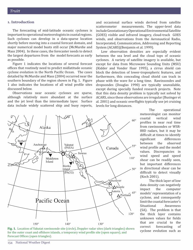
The forecasting of mid-latitude oceanic cyclones isimportanttooperationalmeteorologistsincoastalregions.Such cyclones can develop in a data-sparse locationshortly before moving into a coastal forecast domain, and majornumericalmodelbustsstilloccur(McMurdieandMass2004).Inthesecases,theforecasterneedstodetectthe largest departures from the model forecasts as early aspossible. Figure 1 indicates the locations of several forecastofficesthatroutinelyneedtopredictmidlatitudeoceaniccycloneevolutionintheNorthPacificOcean.ThecasesdetailedbyMcMurdieandMass(2004)occurrednearthesouthernboundaryoftheregionshowninFig.1.Figure1 also indicates the locations of all wind profile sitesdiscussedbelow. Observations near oceanic cyclones are sparse,although relatively more abundant at the surface and the jet level than the intermediate layer. Surfacedata include widely scattered ship and buoy reports,

Fig. 1.LocationofYakutatrawinsondesite(circle),Dopplerradarsites(darktriangles)shownfortheoutercoastandoffshoreislands,atemporarywindprofilesite(opensquare),andForecastOffices(opentriangles).

and occasional surface winds derived from satellite scatterometer measurements. The upper-level dataincludeGeostationaryOperationalEnvironmentalSatellite(GOES) visible and infrared imagery, cloud-track GOESwinds, and observations from the Aeronautical Radio, Incorporated,Communication,AddressingandReportingSystem(ACARS)(Benjaminetal.1999). Low observation densities are especially evident between the sea level and the cloud tops of oceanic cyclones. Avarietyof satellite imagery is available, butexcept for data fromMicrowave Sounding Units (MSU)(Kidder and Vonder Haar 1995), a cirrus shield canblock the detection of lower-tropospheric features, and furthermore, this concealing cloud shield can track in phasewith thewave fora long time. Rawinsondesanddropsondes (Douglas 1990) are typically unavailable,except during specially funded research projects. Notethat this data density problem is typically not solved by ACARS,sincetheseobservationsareirregular(Busingeretal.2001)andoceanicoverflightstypicallyusejetcruisinglevelsforlongdistances.

The operationalmeteorologist can monitor coastal vertical wind profiles in near real timefromrawinsondesorWSR-88D radars, but it may bedifficultattimestoidentifysignificant differencesbetween the observed windprofileandthemodelvalues. Discrepancies inwind speed and speed shear can be readily seen, but important differencesin directional shear can be difficult to detect visually(Koch2001).Thethicklayeroflowdata density can negatively impact the computer models’ representation of a cyclone, and consequently limit the coastal forecaster’s Situational Awareness(SA). The problem is thatthe thick layer contains unknown values for fieldsthat are crucial to the correct forecasting of cyclone evolution such as

Using the Thermal Wind Relationship to Improve Offshore and Coastal Forecasts

Volume 32 Number 2 ~ December 2008 155

thebaroclinicity.Forecastersincoastalregionssometimeshave to wait for the cyclone to be onshore before learning howwelltheoperationalmodelsperformed.Largeerrorsaresometimesobserved. The forecaster can learnmuch about a cyclogeneticsystem if a thermal wind observation (TWO) becomesavailable. For example, the baroclinicity can beconveniently estimated (Pettersen 1956). Also, asemphasized in this article, the thermal wind is a measure of the horizontal temperature gradient. Thermal windvalues can be estimated by calculations using a vertical wind profile or a plan-view array of thickness values,provided the geostrophic component is significantlylargerthantheageostrophiccomponent.Thisconditionisoftencalledthegeostrophicapproximation. ThisarticledescribesamethodtoretrieveaTWOfromthe data-sparse layer associated with midlatitude oceanic cyclogenesis. If this TWO is stronger than a numericalmodel value for the corresponding location, then it is associated with stronger subsequent cyclogenesis and surfacewindsthanthemodelforecast.Theseassociationsdo not require measurement of surface pressure, and therefore the method can be applied to the analysis of oceaniccyclonesindata-sparseregions. Our ability to discernwhen andwhere to apply thequasi-geostrophic approximation has significantlyimproved over the last 60 years. Forsythe (1945)described how the approximation seemed valuable for calculating thermal wind values, but also mentioned thatupperairanalystsexperiencedunexplainedfailures.Thequasi-geostrophic approximationhassubsequentlybeen deemed “generally useful” (Neiman and Shapiro1989)withexceptions that fit into five categories:deepconvection, strongly-curved geopotential height contours, pronounced orographic barriers, the boundary layer, and jetstreakentranceandexitregions.NeimanandShapiro(1989) and Koch (2001) have used the thermal windequation to retrieve horizontal thermal gradients in cases involving upper tropospheric jet stream frontal zones.Neiman and Shapiro (1989) used single-station hourlyprofiler observations to estimate thermal gradients andtheir associated temperature advections in the vicinity of barocliniczones.TheyelaborateontheseminalarticlebyForsythe(1945),andidentifycaseswherequasigeostrophyshould not be assumed. Koch (2001) used mesoscalemodels and products from the WSR-88D, including athermal-windmethodappliedtotheVerticalWindProfile(VWP) data, to study a split front and the associatedconvective rainband in the southeastern United States.He compared the measurements to mesoscale modelforecasts and evaluates the usefulness of the geostrophic assumption. His case study depicts a quasi-geostrophic

partofajet-frontsystemreachingaWSR-88Dsitebeforethearrivalofsignificantageostrophicfeaturesclosertoajetstream. Expanding on this thermal-wind approachusing theVWP and rawinsonde data, an analysis technique forlandfalling cyclones is presented here, where baroclinicity is estimated over thick layers from the troposphere above theboundarylayer.Thesemeasurementsareusefulevenif onlyaccurate towithinone significant figurebecausethat issufficient toalert the forecasterofpossible largeerrorsinthenumericalforecasts.Section2brieflyreviewsthe thermal wind equation and the conversion of potential energy to kinetic energy during cyclogenesis. Section 3explainshowaquasi-geostrophicregioncanbeidentifiedduring midlatitude oceanic cyclogenesis based on the Neiman and Shapiro categories, along with analyses ofscale. In Section 4, we apply the conceptual model tolocations near these cyclones where the thermal wind methodisespeciallyuseful.AcasestudyispresentedinSection 5 to illustrate the usefulness of the technique,followed by a frequency of use evaluation in Section 6.Section 7 is a discussion with suggestions for furtherresearchandSection8givestheconclusions.

2. Thermal Wind and Evaluation of Cyclogenesis During the approach of oceanic cyclones, coastalwind profiles and satelliteMSUs offer the possibility ofretrievingmodel-independentthermalwindvalues.Ifthethermal wind is a valid indicator of cyclone intensity, the retrieved data can be compared to numerical model values of thermal wind and therefore indicate the accuracy of the modelforecastofcyclogenesis,includingthewindfield. Thethermalwindisdefinedasthevectorsubtractionof a lower-level geostrophic wind from an upper-level geostrophicwind.

VT Vg(pu)–Vg(pl)(1)

whereVTisthethermalwindvector,Vg is the geostrophic wind, pu and pl are two pressure levels, and pu < pl.VT can be estimated fromwind profile and sounding data if aquasi-geostrophicapproximationismade. Usingthedefinitionofgeostrophicwind,thethermalwind may also be expressed as:

VT= 1 k X(Φu–Φl)(2) whereΦ is thegeopotential, f is the Coriolis parameter, and k is the unit vector along the z-axis (vertical).

f— ∇

Truitt


Equation (2) can be used for calculating thermal-windvaluesfrommodelthicknessfields,Φu-Φl. A schematic example of how these equations might be appliedtoacyclogeneticsystemisshowninFig.2(afterYoungandGrant1995,Fig.5.1.4a),wherethemagnitudeofthe thermal wind is proportional to the thickness gradient and the length of the arrowwould increase (decrease)as the thickness gradient increases (decreases). Thisfigurealsoillustratesthatthethermalwindisparalleltothicknesscontours,withlowervalues(coldair)totheleftof the vector, and that its strength is proportional to the magnitudeofthethickness(thermal)gradient. Figure2alsocontainsacalloutthatgraphicallyappliesEq.(1),andtheoutlinedarrowisthesamevectorasthatshownwithinthethicknessfield.ThereforeFig.2depictshow the shear of geostrophic winds can be used to calculate the horizontal temperature gradient. This gradient, andhow it might change, has diagnostic value including that an increase in the horizontal temperature gradient provides additional potential energy to a perturbed state thatisavailableforconversiontokineticenergy(Carlson1991).Thisobservationofthicknessgradientcanalsobecomparedtothenumericalmodelvaluebytheforecaster. Assume that we have a loop of satellite imagery

thatendswithacloudpatternasdepicted inFig.2andthatthese imagesagreewithnumericalmodel fieldsforthe cyclone’s track and upper-tropospheric features, includingthesizeandshapeofthecloudshield.Furtherassume that GOES cloud-track winds and ACARS alsocorroboratethenumericalmodelsolution.Weonlyhavethe numerical model data to depict the deep layer between thecirrusshieldandtheoceansurface. Theproblemisthat the data ingested by the model has been limited since the cloud shield developed and began to travel in phase with theperturbation. Wearedependingon themodelto simulate a variety of physical processes, including the conditionswithinthegrowingvoidofobservationaldata.While not a closed system, the kinetic energy of a cyclone derives from the available potential energy released in the rearrangement of the air masses (Reed 1990), andthe numerical model provides an approximation of this processalongwiththesubsequentwindfield. The model simulation of the processes in thehidden layer may become less representative of the real atmosphere, as time passes and the void of observational datapersiststhroughadditionalmodelruns. Therefore,observationaldataarestillsoughtfromthehiddenlayer. If thermal-gradient observations then becomeavailable from underneath the cloud shield, they can show whether the potential energy available for cyclogenesis is significantly higher than the model depiction. If asignificant amount of that higher potential energy isconverted to kinetic energy in the cyclone, then the resulting surface winds should be consistent with having higherkineticenergythanthemodel.Basedonforecasterexperience, such changes typically include higher wind speedsinthelowertroposphereandatthesurface.CasesalsooccurthataresimilartothedepictionsinMcMurdieandMass(2004)wherethesubsequentcycloneevolutionistoodifferentfromthenumericalmodelsolutiontobeusefullycompared. The forecaster will prefer computer model(s) witha representative simulation of the potential energy available for that conversion. If the values retrievedfromobservations using Eq. (1) are significantly higherthan the values predicted by the models using Eq. (2),the forecaster will subjectively strengthen the model solution. Suchacomparison technique isusefuleven ifthe observational data are at a single location because the most important cyclone mechanisms are synoptic-scale processes(ParsonsandSmith2004). The literature has long mentioned cases where Eq.(1)wasappliedtoactualwindswitha“lackofsuccess”(Forsythe1945).Suchfailuresresultfromsourcesoferrordescribed by Neiman and Shapiro (1989). The largestsources of error would be from the presence of one or more

Fig. 2.Schematicshowingaleafcloud(stippling)duringcyclogenesis(afterYoungandGrant1995,Fig.5.1.4a,p.208)withadditionalconceptualmodeldetails(afterHolton1992,Fig.6.5).Mid-levelcloudE(hatching)hasemergedfromundercirrusshieldF(stippling)betweenjetstreaksJ1andJ2(arrowheads).Upper-levelstreamlines(longarrows)indicateflowthroughshort-wavetroughaloft(dashedline).Surfacefronts(conventionalnotation)showaninflectionpoint.Thicknessbetween the streamlines is shown as heavy dashed lines, with athermalwindvector(outlinedarrow)consistentwiththelocalthicknessgradientatthevectors’base.Figurecalloutillustratestherelationshipofthethermalwind(outlinedarrow)tothegeostrophicwindsat850and500mb.



of the five categories of strong ageostrophy. Additionalerrors should result from the application of Eq. (1) inplaceofthecompletethermalwindequation(NeimanandShapiro1989),butconsistentwithForsythe(1945),sucherrorsshouldbeanorderofmagnitudesmaller.Thereforethe forecaster would benefit from a diagnostic methodthat checks the validity of the geostrophic approximation fortheobservedwindprofiles.

3. Regions Containing Strong Ageostrophy

Considering thermal wind observations in real-time begins by first seeking to identify a sector within theoceanic cyclone that has the associated baroclinicity, yet where the actual winds have a geostrophic component significantlylargerthantheageostrophiccomponent.Thissection shows that the strong ageostrophies near such cyclonesaresufficientlylimitedinspatialscale,suchthatan adjacent sector suitable for the geostrophic assumption andcontributingtocyclogenesiscanbeidentified.

a. Synoptic-scale regions containing strong ageostrophy

The Neiman and Shapiro (1989) exceptions to thevalidity of the quasi-geostrophic assumption can be identifiedusingdataandtechniquesalreadyavailabletooperationalmeteorologists: (1)Deep convection can bedetectedusingsatellite imageryorWSR-88Dreflectivitydata. (2) Strongly curved geopotential height contours,along with other sources of error such as data corruption duetovelocityaliasing,shouldbedetectableusingWSR-88D velocity data displayed with the VWP root meansquared error (RMSE). (3) Pronounced orographicbarriers on the outer coast can produce barrier jets that arenotsignificantabovetheterrainlevel(Parish1982).(4)Boundarylayereffectsoveroceansandshallowcoastalterrain can typically be neglected by not using data below the 850-mb level; however, a method for forecastingsurface wind must still account for a transition through theboundarylayer. Theremainingexceptiontothevalidityof thequasi-geostrophicapproximation(NeimanandShapiro1989)isfromupper-leveljetstreaks.Thelocationofajetstreamand the existence of jet streak entrance and exit regions areeasily identifiedusing satellite imagery (KidderandVonderHaar1995).Note that the jet stream is intrinsictocycloneevolution(Reed1990)andthereforeroutinelyexists within synoptic-scale distances of the cyclogenetic baroclinicityfieldoneseekstosample.Consequently,thetopic of the strong ageostrophy associated with jet streaks isemphasizedinthisarticle.Wewillnowuseanexistingconceptual model of cyclone development to identify a sectorwherethegeostrophicapproximationisuseful.

—

b. Scale of strong jet streak ageostrophies

A useful measure of the validity of the geostrophic approximationistheRossbynumber(R0),whichisdefinedas the ratio of the characteristic scales of ageostrophic acceleration to the Coriolis acceleration:

R0 U (3)

fL

where U is the velocity scale, f is the Coriolis parameter, and Listhehorizontallengthscale.TheRossbynumberis typically of order 0.1 for midlatitude synoptic-scalesystems(Holton1992)andoforder1.0inthepresenceofjetstreaksonsubsynopticscales(Bluestein1993). When R0~0.1, the quasi-geostrophic approximationcan be made, although the thermal wind calculation is limitedtoonesignificantfigureaccuracy.AcomparisonoftheresultsofEq.(1)usingwindobservations,withEq.(2)usingmodelthicknessfields,canreveallargeerrorsinthemodelestimateofavailableenergy. Actual measurement of R0 is not practical; however, numericalmodel fieldsofR0 were temporarily available atWFO Juneau, and were applied to the thermal windmethod.CasesofR0=0.2occurred,alongwithonecaseofR0=0.3.Thesecaseshavebeenusedtoestimateathresholdvalueforthesignificanceoftheratioofobservedthermalwindmagnitudeovermodelthermalwindmagnitude.Ifthe ratio is above1.3, then themeasured thermalwindvalue is significantly higher than themodel value, withincreasingvalueshavingincreasingsignificance. In subsynoptic regions where R0~1, Eq. (1) isinapplicable and therefore cannot be used to identify errors in the model estimate of available energy.Furthermore, the vertical coupling of ageostrophic winds associated with isotach maxima can result in the depth of strong ageostrophy extending below the jet-stream level (Bluestein1993).Therefore, Eq. (1) shouldnotbeappliedtowindprofiledatafrombeneaththejetstreaks.These ageostrophies are contained within a subset ofthe cyclogenetic region one seeks to sample for thermal gradients and the geostrophic approximation can be applied to the remainder of the region, as described below withaconceptualmodel.

4. Conceptual Model and Application a. Cyclogenetic regions: quasigeostrophy vs. ageostrophy

An oceanic cyclogenetic system is depicted schematically inFig.2. Thecirrusshield,depictedwiththestippledareaF,iscommonlyidentifiedwithinfraredandwatervaporimagery.Individualjetstreaksalongthe

Truitt


jet stream can be located using loops of such images, but theprecisionofstreakidentificationisbettertransverseof the flowthanalong it. Thedetailsof thetransverse/vertical circulations associated with jet streaks are beyondthescopeofthisarticle.R0~1shouldbeoccurringin the presence of these jet streaks on subsynoptic scales (Bluestein 1993). Similar strong ageostrophies areassumed near where the cirrus shield area F is depicted asadjacentcloudshieldE,butwillbehardertoidentifydue to the complexity of the jet streaks that should soon couple.Thehorizontalextentofthestrongageostrophiesis not known to a subsynoptic-scale resolution, i.e. wecannot correctly draw R0 isopleths for various levels on Fig.2.However,thejetstreakshavelocationsrelativetothe cyclogenetic system that are routinely identified tosubsynoptic scale precision by forecasters using satellite imagery. Suchfeaturesexistonasmallerscalethanthewhole cyclone, and this is consistent with model studies that show the ageostrophic circulations associated with cyclones are typically an order of magnitude smaller thanthegeostrophiccirculations(Anthes1990). Letusassume the modeled cyclones accurately represent actual cyclones.InFig.2thesmallerscaleregionofageostrophiccirculations would include the jet streaks that the forecasteridentifiesinthewesternpartofthecyclone. Because the geostrophic circulations take place ona much larger scale, the thermal wind equations can be appliedusefully.AssumethatthatthecycloneinFig.2isintheNorthPacificandisapproachingaWestCoastWSR-88D orwind profiler. Such a location under the cirrusshield is useful because of: (1) the obscuration by thecirrusshield,(2)theroleofthethicknessfieldincycloneevolution,and(3)thejetstreaksarestillasynopticscaledistanceoffshorefromthewindprofilesites. Theflowbecomesmoreageostrophicasthejetstreaksmovewithinsubsynoptic-scalerangeofthewindprofilesite,andtheforecastercananticipatethisbyusingGOESsatellite imagery or cloud motion winds to track the jet steaks synoptically. Therefore,when the jet streaksarewithinsubsynopticrangeofthedatasitetheTWOperiodhasended.AtabularhistoryoftheTWOsisuseful. Forexample,datafromtheWSR-88DsitePACG(BiorkaIsland)(Fig.1)isrecordedalongwiththeapplicationofEq.(1)byacomputerscriptatWFOJuneau.Theforecastercanthenreviewapriorperiodofwinddatacollectedsufficientlyfarahead of these west coast land-falling strong ageostrophies thatthequasi-geostrophicapproximationisvalid. b. Forecasting oceanic cyclogenesis and surface wind

A diagnosis of cyclogenesis can be made by blending satellite data, conceptual models, numerical model

solutions,andobservationsincludingthermalwind.Theforecaster blends experience with a conceptual model of cyclogenesis that includes the conversion of potential energy to kinetic energy (Bluestein 1993). Usually, thethermal wind estimate calculated from wind profileswith Eq. (1) agrees to one significant figure with thecorresponding numerical model solutions calculated with Eq.(2),whichshowsthatthenumericalforecastrepresentstheenergyconversionabouttooccur.However,astrongerthermal wind is associated with stronger cyclogenesis than the numerical model solution, and stronger cyclogenesis isassociatedwithstrongersurfacewind.Insuchacase,the forecaster must adapt his or her analysis, as illustrated inthefollowingexample.

5. Forecast Shift Case Study

Thiscasestudyfrom11January2002atWFOJuneauillustrates how the forecasting of winds associated with an oceanic cyclone during coastal approach can be improved with a baroclinicity calculation that provides analert. TWOswerecalculatedwiththePAYA(Yakutat)rawinsondeand thePACGWSR-88Dwindprofiles. TheWSR-88D site was temporarily out of service when ameasure of baroclinicity was first needed. The PAYArawinsondewasfirstusedbytheforecastersforthewind-shearcalculationandcomparisonwithmodeldata. Theforecasters issued amendments based on these data, and then began to receiveWSR-88D VWP data, which theyusedforupdatedevaluations.Thewindspeedunitsusedinthissectionforthepublicforecastsandverificationaremph(ms-1),whilekt(ms-1)wereemployedforthemarineforecastsandverification..Table1showsthechronologyofeventsthatoccurredduringtheforecastshift. a. Real-time vs. hindsight calculations

Twothermalwindcomparisonsareprovidedineachcase. First is an initial crude comparison used in real-time during the forecast shift; secondly a more stringent comparisonisappliedlaterinhindsight. Duringtheforecastshift,themagnitudeofthethermalwindcalculatedwithEq.(1)fromthe850-500mbPAYAandPACGwindswerecomparedwiththemagnitudeofthethermalwindcalculatedwithEq.(2)fromthe1000-500mblayerAviation(AVN)data.The5000ft(1524m)PACGmeasurements were the lowest available winds due to the boundary layerconstraint. HindsightcalculationsusingtheAVN850-500mblayerareprovided.



b. Forecast shift briefing AGOESIRanimationendingwiththeimageat0000UTC11January2002(Fig.3)indicatedcyclogenesisanda northward track. The 0000 UTC National Center forEnvironmental Prediction (NCEP) surface map (Fig. 4)showedasurfacelowat53ºN,143ºW.Thedifferencesamong the models were small, but the model of choice bythepriorshiftwasthe1800UTC10January2002runof the AVNGlobalModel and had therefore guided theforecastpackageissuedtousers.Outputfromthismodelrunat6h,12h,and18hisshowninFigs.5-7.Figure5showsAVNthermalwindvaluesavailableclosesttoPAYAandPACG,aswellasthecorrespondingmodelthicknessfieldat6h.Figure6showsthesamemodelfeatures,withtheadditionofthesurfacepressurefieldandthelowthatistrackingnorthat12h.Figure7showsthesamemodelfeaturesasFig.6,exceptforthethermalwindvaluesareomittedastheyarenolongerusedforcomparison,at18h.Forecastersbelievedthatthesatelliteimageryshowedupper-tropospheric cyclogenesis with weak development in the lower troposphere, but the view was blocked by the extensivecloudshield(Fig.3).AnotherproblemwasthatthePACGWSR-88Dsitewasoutofserviceuntil0308UTC.The0000UTCPAYArawinsondewasavailablebutneededevaluationforusabilitywiththegeostrophicassumption.Therefore,thevalidityofthegeostrophicassumptionfirstneededtobeestablished.

Fig. 3. InfraredGOESimagefor0000UTC,11January2002.Capital L denotes approximate location of sea-level pressure minimum.

Fig. 4. 0000UTC,11January2002NCEPsurfaceanalysis.Solidcontoursareisobars(mb).Dashedlineindicatesthe pressure trough, and capital L’s denote approximate locations of sea-levelpressureminima.Standardsymbolsdenotefrontalboundaries.PAYArawinsondesiteisshownasopencircle.Table 1. Chronologyofforecastshift11January2002

Time (UTC) Event1800 LastAVNmodelrunon10January20020000 Rawinsondesarecompleted,Fig.4.maptime0020 Marineforecastissued0030 Zone forecast issued, including Yakutat0100 Forecasting crew change and notes started

~0145 PAYArawinsondedataareusedforcalculationofther-malwind,Eq.(1)

0206 Marineforecastisamended0211 Wind Advisory issued for Yakutat zone0308 PACGdatabeginstoarrive,includingVWP0313 PACGVWPdataareusedforcalculationofthermalwind,

Eq.(1)~0330 PACGWSR-88Ddatadiagnosedavalidationofthe

amendments0600 AVNmodelverificationtime(Fig.6b)0943 PAYAfirst45mph(20ms-1)gust1200 ShipWCZ6534verifiesGale1242 PAYAgustof46mph(21ms-1)

Truitt


Fig.5.AVN6-hforecastof1000-500mbthicknesscontours(dashed,dam)andthermalwindvectors(kt),validat0000UTC11January2002.LocationsofPAYArawinsondesite(opencircle)andPACGWSR-88D(darktriangle)areincluded.

Fig.6.AVN12-hforecastofsea-levelpressure(solid,mb),1000-500mbthicknesscontours(dashed,dam),and850-500mbthermalwindvectors(kt),validat0600UTC11January2002.CapitalLindicateslocationofmodelsea-levelpressureminimum.LocationsofPAYArawinsondesite(opencircle)andPACGWSR-88D(darktriangle)areincluded.

c.Applicability of the geostrophic approximation

The satellite imagery showed a baroclinic commacloudwithanupper-level inflectionpointinthevicinityof54ºN,145ºW(Fig.3).Jetstreamsignaturesextendedupstream to the south, but not downstream toward the coastincludingPAYAandPACG.Basedontheconceptualmodel of jet streaks with ongoing cyclogenesis, we assumed

thattheflowoverthecoastalregionandadjacentoceanwasquasi-geostrophic.Thesatelliteimageryat0000UTCdidnotshowconvectionalongtheoutercoasttotheNNEthroughEofthecyclone.Basedontheconceptualmodel,thesatelliteimagery,andexperienceusingthePAYAdata(Truitt1994),wedecidedthatthebaroclinicitycouldbecalculatedusingthePAYAwindshearsandEq.(1). ThePACGWSR-88Dbecameavailablewith the0308UTCvolumescan(Fig.8).BasedontheAVNcyclonetrack(Figs. 6 and 7), the forecaster assumed that jet streakageostrophies would not reach the outer coast until many hourslater. TheRMSEvaluesforthewindsinFig.8(notshown)were less than 4 kt, which is consistent with a near-homogeneous wind field at all levels. We thereforeassumed the PACG data shown in Fig. 8 to be quasi-geostrophic.

d. PAYA rawinsonde

The 0000 UTC PAYA rawinsonde 850-500-mb layerthermal wind was compared to the corresponding model solution to establish whether cyclogenesis should generally follow theAVNprediction. ThePAYA thermalwindusingEq.(1)was52kt(27ms-1).TheAVNthermal-windmagnituderetrievedwithEq.(2)was25kt(13ms-1)andthisvalueisoverlaidonFig.5.Themagnitudeofthe thermalwindatPAYAwas thereforeroughlydoublewhatthemodelpredicted. As of 0000 UTC, the PACG WSR-88D was not yetreporting.Theforecasterusedthreefactorstosubjectivelyestimate that the thermalwind near PACG wasabouthalf again what the model guidance showed: (1) ThePAYAthermalwindobservationhadusefulnessforawideareaincludingPACG,butdiminishingwithdistance. (2)Accordingly, the numerical model thermal wind values needed to be factored in more for increasing distances from the PAYA data site. (3) The satellite imagerywasusedtoestimatethesizeofthecyclogeneticsystem.

e. PACG WSR-88D VWP

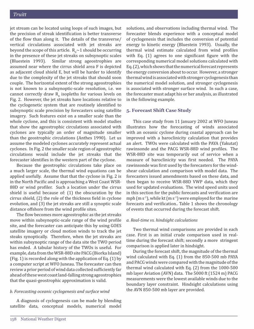
The VWP from PACG (Fig. 8) first became availablejustafter0300UTC,11January2002.Thiswasbetweenthe times of the AVN 6 and 12 hour forecasts valid at0000UTCand0600UTC11January2002.Therefore,themagnitude of the thermal wind calculated with Eq. (1)wascomparedwith themeanvalueof theAVN thermalwindmagnitudes. We used the VAD (Velocity AzimuthDisplay)windat5,000ft(1524m)asanapproximationforthe850mbwind,andtheVADwindat18,000ft(5486m)asanapproximationforthe500-mbwindinEq.(1).



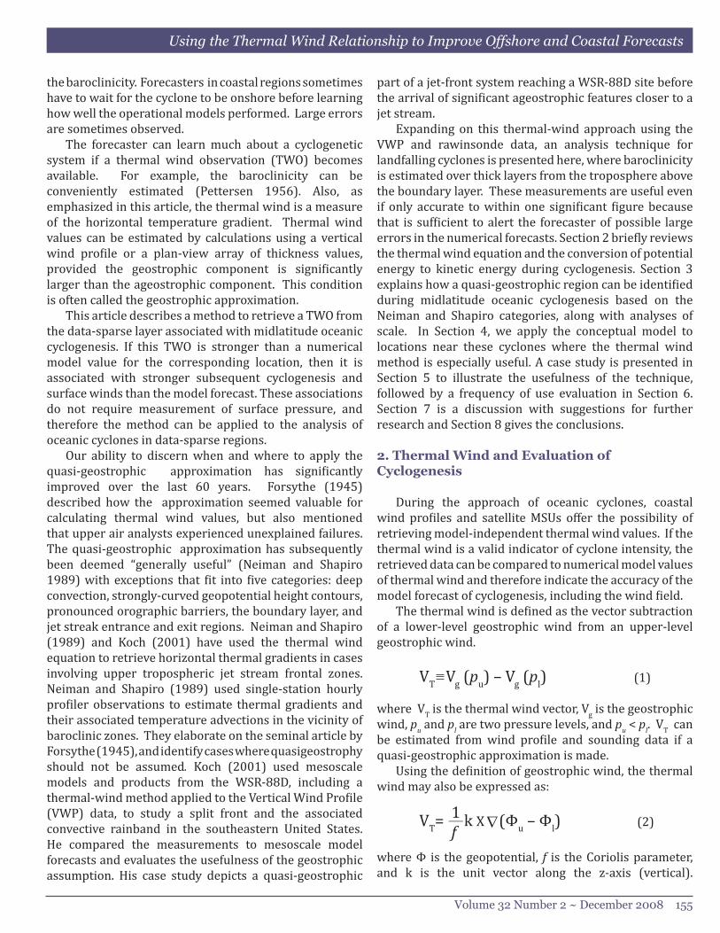
Basedonthesewindsobservedat0313UTC,thethermalwindatPACGwasfoundtobe39kt(20ms-1),whiletheAVN thermal-wind magnitude for PACG was 25 kt (13m s-1). This corresponds to a ratio of 1.5 between themeasuredvalueandthemodelvalue.Basedonforecasterexperience, the stronger cyclogenesis would result in peak surfacewindsnearPACGnearly50%strongerthanthosepredictedbytheAVN.

f. Amendments issued and verification received TheYakutat Public Zone from0020UTC11 January2002stated“windsbecomingsoutheastto25mph(11ms-1)bythemorning(of11January).”At0211UTC,aWindAdvisory was issued for the Yakutat Zone and the text wasamendedto“Southeastwindsincreasingwithguststo50mph(22ms-1)”fortheovernightperiod.At0943UTC,thewindsatPAYAbecamesoutheastandincreasedto24mph(11ms-1).From0953UTCto1153UTCfourpeakwindvaluesof45mph(20ms-1)occurred,andthehighestwindof46mph(21ms-1)occurredat1242UTCand1253UTC. Marineforecastsreceivedcorrespondingamendmentsat0206UTC.Onlyonemarine observation was to become availableintheeasternGulfofAlaskathrough1200UTC(Fig.7)andthemarinewindamendmentforthislocationwasbasedonamoreconjecturaluseofthe0000UTCPAYATWO.ThesubsequentPACGTWOcausedtheforecasterstobecomemoreconfidentthatthepreviouslytransmitted0206 UTC marine amendment was appropriate forthe easternGulf of Alaska closer to PACG. The originalmarineforecastforthislocation,issuedat0020UTC,read“southeast winds less than 20 kt (10 m s-1) increasingto southeast 25 kt (13 m s-1) Thursday evening,” withThursdayeveningdefinedas0300UTCto0900UTC11

Fig.7.AsinFig.6,except18-hforecastvalidat1200UTC11January2002.NotetheinclusionofthelocationoftheshipreportfromWCZ6534(largeblackdot).

Fig.8.VWPfromPACGfor0308-0358UTC11January2002,asdisplayedontheAdvancedWeatherInteractiveProcessingSystem(AWIPS)attheNWSJuneauWFO.Standardwindbarbsareshowninheightscaleforeach1000ft(305m).SecondcolumnofwindbarbsdepictsVWPendingat0313UTCusedforshearcalculation.Theveeringofwindisevidentforalargedepth.

January2002. The forecasthadnootherwind increaseovernight. Themarineamendmenttransmittedat0206UTCread“southeastwindsincreasingto40kt(21ms-1)Thursdayevening.” At1200UTC11January2002,shipWCZ6534 reportedwinds southeast at 40 kt (21m s-1)(Fig.7).Inbothcases,theTWOhadimprovedthesurfacewindforecast.

g. Hindsight computations

The case study above described the calculationsmade during a forecast shift: a comparison of thermal windvaluesretrievedfrom850-500-mbobservedwindswith the thermal wind values calculated from the AVN1000-500-mb thickness. In hindsight, a comparison ofthermal wind values retrieved from 850-500-mb PAYAwinds(52kt,or27ms-1)withthethermalwindvaluescalculatedfromtheAVN850-500-mbthickness(19kt,or10ms-1)yieldsaratioof2.7. Acomparisonof thermalwindvaluesretrievedfrom850-500-mbPACGwinds(39kt, or 20 m s-1) with corresponding AVN 850-500-mbthermalwind(19kt,or10ms-1)yieldsaratioof2.0. NotethatusingtheAVN850mblevelinsteadof1000

Truitt


mbreducedthethermalwindfrom25kt(13ms-1)to19kt(10ms-1),whichincreasedtheratioto2.7.Theresultsvalidatethebaroclinicityalertissuedduringtheshift.

6. Rates of Occurrence

Casestudieswereloggedduringanearlyperiod(coolseason of 1999-2000) in the techniques development.During this period, the forecasts used the TWOs as apredictor of surface winds for any cases where landfalling featuressuchascold frontsmightresult inasignificantwindevent. Thesecasesare identifiedandincludedforthe purpose of completeness. This broad applicationof the thermal wind method was based on a statistical study (Truitt 1994). The case studies typically did notdifferentiate between the marine forecasts and theforecastsforcommunitiesnearsealevel.Thecaseswereclassifiedintothefollowinggroups:

1) The TWO values were significantly higher thanthe numerical models (similar to the above casestudy).Thesurfacewindswereforecastandverifiedas significantly stronger than numerical modelpredictions(twocases).

2) The numerical model solutions had significantlydifferentwindforecasts.Thethermalwindmethodwas used to choose the model with stronger winds anddidverify,includingaHighWindWarning(onecase).

3) The thermal wind agreed with numerical modelvalues and the documentation then ended (ninecases). Intwoof thecasesthere is indicationthatthe forecaster did not expect cyclogenesis, but this detailisdifficulttoreconstruct.

4) The thermal wind was weaker than any modelsolutions and explosive cyclogenesis occurred as verifiedwithshipdata.Theforecasterssuccessfullyapplied the model solutions presumably using satellite imagery and other standard tools. Themethodfailed(onecase).

5)The thermal wind method was applied duringobvious convection after a log entry of ‘could these cellsbesevere.’ Themodelsdepictedcyclogenesisand forecast winds were raised higher than numericalmodelsolutions. Theverificationoftheresulting wind advisory was claimed based on one gustbuttheloghasambiguity.Themethodshouldnothavebeenapplied(onecase).

6) No cyclone, based on the available hardcopiesofmodel analysis and GOES IR. A cold frontwasapproaching at the time of application of the thermal windmethod.Theratioofthermalwindovermodelvalues was 1.33. No documentation was foundthat indicatedwhether the forecasts differed frommodel depictions, or whether verification becameavailable.Themethodshouldnothavebeenapplied(onecase).

The number of cases here is too small for formalstatistical analysis, but subjective comparisons with the subsequent seven years are practical. The first threecategorieshavetypicalrelativefrequenciesofoccurrence.Failures have subsequently occurred but not for the reasons given in 4, 5 and 6. The subsequent failureshave occurred when winds, stronger than depicted by the numerical models, occurred at high elevations in the interiormountains. Failuressuchas(4)shouldsometimesstilloccur.Thethermalwindmethodonlysamplesthe850-500mblayer,anddoesnotidentifyuppertroposphericfeatures. Skillisnot claimed for caseswhere theTWO isweaker thanthe numerical model values, and they may result from layers with stronger thermal wind values either above or below the 850-500 mb sample layer. In (4) above,the forecasters used the model guidance and standard techniquessuccessfully. CaseswhereTWOsarestrongerthanthemodelvaluescan have actual cyclone evolutions that differ from themodelsolutionsinavarietyofways.Thestrongersurfacewinds can occur in locations that seem inexplicable using themodelsolutions. Suchcasesarehardtoclassify,butareroughlysimilartoMcMurdieandMass(2004). 7. Discussion and Proposed Future Research

In this study thedata-sparse layerassociatedwithamidlatitude oceanic cyclone was sampled for a thermal wind calculation, from which the forecasters had inferred that the cyclogenesis was to become stronger than predictedbyoperationalcomputermodels.Theforecastswere updated, and the updates monitored, with the expectation that an increase in wind speeds would reach thesurface. This simple method should help provide directionto the research and numerical modeling communities.What the operational community needs most is for the numerical model performance to improve enough for suchmethodstobeobsolete. Therefore,suggestionstothe research community are provided, including some for futuretheoreticalwork.



For example, the numerical modeling community could research the creation of model ensembles that emphasize a range of thermal wind values and their subsequent cycloneevolutions. Thetheoryofextratropicalcyclones(Hoskins1990)extendsfarbeyondthemethodpresentedin this article, albeit themethod is convenient for fieldoperations. Based on the literature (Carlson 1991; Reed 1990)wecantypicallyexpectstrongerwinds,orasignificantlyaltered cyclone evolution when there is stronger thermalwind in the cyclogenetic region. TheTWOandcomparison tool is designed to calculate thermal wind from observations and compare it with the numerical model solution. Tests at the WFO Juneau demonstrateexperimentally that we can improve our forecasts with this tool. Consequently, the reasoning was right andfuture work should investigate the mechanisms behind the relationship, as well as the reasons for the observed thermal wind values being stronger than the numerical modelsolution. TheTWOandcomparisontoolusesseveralsimplifyingassumptions but introduces error, especially when the observedvaluesarestrongerthanthemodelvalues:(1)Theexistingnumericalmodelresultsaretypicallyappliedwith the assumption that the cyclone evolution will have little change except for the subjectively determined increases in wind speeds in the lower troposphere and the surface. (2) The increased thickness gradientmay have several unknown causes. However, theyare unknown and the result is the assumption that no differentiation exists that may affect cyclone evolution.(3) The complete thermal wind equation is not used,and most of the additional terms should be practical to implement (Neiman and Shapiro 1989). (4) The tooldoesnotaccountforboundarylayercomplexities.Theseinclude friction, stratification, baroclinicity, turbulence,along with their interactions. In addition, the sensibleand latent heat fluxes in the boundary layer can “fuel”the rapid development of oceanic extratropical systems (Uccellini1990).ThedatausedforEq.(1)needtocomefromabovetheboundary layer, yet the associated method must account for processes that transport momentum downward through theboundary layer to the surface. In addition,thecoastalwindprofilesitesaretypicallylocatedwherethe surface roughness changes from water to land and a deeper boundary layer. For example, experience inoperational meteorology indicates the boundary layer overtheoceanisbelow3000ft(914m).However,testsusing the PACGWSR-88D VWP show higher RMSE andobviousexceptionstohomogeneousflowthrough4000ft(1219m).Analtitudeof5000ft(1524m)isassumedto

be above the boundary for the purposes of the thermal windtool,yetweakorographicinfluenceshaveprobablybeendetectedatPACGevenduringonshoreflow. Thecasestudiesfrom1999-2000didnotshowmethodfailures that have been observed in the following seven years. These subsequent failures have occurred whenwinds stronger than depicted by the numerical models were forecast, but the onlywinds significantly strongerthan the models occurred at high elevations as reported byanemometers in the interiormountainsnear Juneau.In such cases themethod seems to predict an increasein a cyclone’s winds aloft that do not extend downward through the boundary layer until reaching topography aboveabout4000ft(1219m). CaseswheretheTWOisweakerthanthenumericalmodel values cannot be usefully applied. It is possiblethatastrongbarocliniclayerextendsbelow5000ft(1524m)thatthenumericalmodeldepictsasbeingwithinthe850-500mblayer. Ifthisisso,itisalsopossibleforthetool to fail to detect cases where the numerical model surfacewindswillnotbestrongenough. The persistent void of observational data offshoremay require soundings for significant improvement ofnumerical model performance. Dropsondes (Douglas1990)couldbeplacedoffshoreaccordingtotheconceptualmodelandsynchronizedfornumericalmodelruns.TheTWOscouldalsobecalculatedusingwindsatlowerlevelsthan ispracticalatsites likePACG,dueto theshallowerboundary layer over the ocean. Rapid changes areoccurringinthefieldofUnpilotedAircraftSystems(UAS)thatshouldlowerthecostpersounding. SatelliteMSUscanalsoretrievedatathroughclouds(KidderandVonderHaar1995).Acomparisonwouldbemadebetweentwoapplications of Eq. (2): the first usingmodel thicknessfields, the secondusing a fieldof thickness values fromtheMSUsoundings. This secondapplicationofEq. (2)wouldusefinite-differencingtoobtainthefieldofΦu-Φl forlocationsaccordingtotheconceptualmodel. While the conceptual model presented above has broad operational applicability, the following limitations should be noted: (1) The complex terrain of westernNorth America often generates strong ageostrophies atthe data site if the cyclone is making landfall to the south, orifthecycloneisfollowingacoastaltrackfromthesouth.(2) The exact location of the jet streaks and associatedageostrophy can be difficult to determine. Cases havebeenobserved atWFO Juneauwhen thewindbegan toback with height earlier than expected and are believed to be associated with ageostrophic frontal transverse circulations as described by Koch (2001). This earlyarrival of ageostrophies may be associated with mature occlusionsasdefinedintheNorwegianconceptualmodel

Truitt


of cyclone evolution. (3) Measurements at a data sitecancorrespondtoaprecedingbaroclinicwave. (4)Thethermal wind for the 850-500-mb layer should also becalculated in two or more layers, such as 850-700 mband700-500mb,tohelpidentifycaseswherethestrongthermal wind and baroclinicity could be limited to the upperlayer,withoutextensiontotheboundarylayer.

8. Conclusion

Historically, meteorologists have thought of thethermal wind as an elegant instruction tool, but much less asausefulanalysistool.Thegeostrophicapproximationhas a long history of failures (Forsythe 1945; Doswell1991),andstrongageostrophiesaresignificantfeaturesofextratropicalcyclones.However,theidentificationofsuchageostrophies has becomemore practical (Neiman andShapiro1989)andallowstheidentificationofasynoptic-scale region within the cyclogenetic system suitable for thequasi-geostrophicapproximation.Theregionsuitablefor assuming quasigeostrophy includes a low data-density volume under the cloud shield that travels in phase with thecyclogeneticwave.

TheTWOiscomparedtothenumericalmodelvalue.If the observation is significantly stronger than themodel value, then at least one of three model-relative outcomes will occur: (1) raised wind speeds in thelower troposphere, (2)higher surfacewindspeeds,and(3) subsequent cycloneevolution toodifferent from themodelforoperationallyusefulcomparison. For operational meteorologists, the thermal wind methodcanalerttheforecastersofsignificantnumericalmodelforecasterrors.Thatsuchasimpleapproachcanpredict numerical model errors should help provide direction to the research community. For the researchcommunity, the thermal wind method described, emphasizes the need for sounding data (from satellitesmicrowavesensorsoraircraft)withinoceanicmidlatitudecyclogeneticsystems.

Author

Jim Truitt is a Lead Forecaster at NOAA/NationalWeather Service Forecast Office in Juneau. He earnedaB.S. inMeteorology fromTexasA&MUniversity. Hislong-term goals include improving the wind forecasting of extratropicalcyclonesintheNorthPacific.

References

Anthes,R.A., 1990:Advances in theunderstandingandprediction of cyclone development with limited-area fine-mesh models. Extratropical Cyclones: The Erik Palmén Memorial Volume, C. W. Newton and E. O.Holopainen,Eds.,Amer.Meteor.Soc.,221-253.

Benjamin,S.G.,B.E.Schwartz,R.E.Cole,1999:AccuracyofACARSwindandtemperatureobservationsdeterminedbycollocation.Wea. Forecasting,14,1032-1038.

Bluestein,H.B.,1993:Observations and Theory of Weather Systems. Vol 2, Synoptic-Dynamic Meteorology in the Midlatitudes, OxfordUniversityPress,594pp.

Businger,S.,M.E.Adams,S.E.Koch,andM.L.Kaplan,2001:Extraction of geopotential height and temperaturestructure fromprofilerand rawinsondewinds. Mon. Wea. Rev.,129,1729-1739.

Carlson, T. N., 1991: Mid-Latitude Weather Systems. HarperCollinsAcademic,507pp.

Doswell, C. A., III, 1991: A review for forecasters onthe application of hodographs to forecasting severe thunderstorms.Natl. Wea. Dig.,16(1),2-16.

Douglas,M.W.,1990:Theselectionanduseofdropsonde-equipped aircraft for operational forecasting applications.Bull. Amer. Meteor. Soc.,71,1746-1756.

Forsythe, G. E., 1945: A generalization of the thermalwindequationtoarbitraryhorizontalflow. Bull. Amer. Meteor. Soc., 26,371-375.

Holton,J.R.,1992:An Introduction to Dynamic Meteorology. 3d.ed.AcademicPress,511pp.

Hoshkins, B. J., 1990: Theory of extratropical cyclones.Extratropical Cyclones: The Erik Palmén Memorial Volume, C.W.NewtonandE.O.Holopainen,Eds.,Amer.Meteor.Soc.,64-80.

Kidder, S. Q., and T. H. Vonder Haar, 1995: Satellite Meteorology: An Introduction. Academic Press, 466pp.

Koch,S.E.,2001:Real-timedetectionofsplitfrontsusingmesoscalemodelsandWSR-88Dradarproducts.Wea. Forecasting,16,35-55.



Acknowledgments

TheauthorwishestothankthetworeviewersfortheNationalWeatherDigestfortheirconstructiveandhighlydetailedcommentsaboutthemanuscript.Theyprovidednumerousneededrecommendations.They are Dr. Jerome Patoux, Professor ofMeteorology at the University ofWashington, Seattle, andDr.ScottRochette,AssociateProfessorofMeteorologyattheStateUniversityofNewYork(SUNY)atBrockport.

Dr. David Schultz, National Severe Storms Laboratory, provided both encouragement and an extraiterationduringapriorreviewprocessthathelpedtightenthescienceandthetext.ConversationswithJohnWeaver,ResearchMeteorologistatNOAA,andDanBikos,ResearchCoordinatorfortheCooperativeInstitute for Research in the Atmosphere, helped the cyclogenesis presentation. Tom Ainsworth,MeteorologistInChargeatWFOJuneau,providedsuggestionstohelpreadabilityaswellasoperationalapplication.GaryHufford,NWSAlaskaRegionalScientist,andAudreyRubel,PhysicalScientist,providedajointmanuscriptreviewandseveraloftheirrecommendationshavebeenapplied.

SarahOlsenservedascomputergraphics illustrator. AxelGraumann,meteorologistandHeadof theSatelliteServicesGroupwithintheNationalClimaticDataCenter,providedtheGOESIR image. PaulShannon,thenLeadForecasterandcurrentlytheInformationTechnologyOfficerinJuneau,wrotetheWSR-88DVWPscript.CarlDierking,ScienceandOperationsOfficer in Juneau,wrote theapplicationusedtologforecasternoteswithintheAWIPSenvironment,andprovidedadetailedreviewwithseveralchangesthathavebeenapplied. GaryEllrod,ChiefEditorofNationalWeatherDigest,encouragedelaborationonthepossiblesatelliteapplicationofthemethod.HeandKermitKeeter,TechnicalEditorofNationalWeatherDigest,providedfinishingreviewsthataddedtothetext’sclarity.

McMurdie,L.,andC.Mass,2004:Majornumericalforecastfailuresover theNortheastPacific. Wea. Forecasting, 19,338-356.

Neiman,P.J.,andM.A.Shapiro,1989:Retrievinghorizontaltemperature gradients and advections from single-stationwindprofilerobservations.Wea. Forecasting, 4, 222-233.

Parish,T.R.,1982:BarrierwindsalongtheSierraNevadaMountains. J. Appl. Meteor.,21,925-930.

Parsons, K. E., and P. E. Smith, 2004: An investigation

of extratropical cyclone development using a scale-separationtechnique.Mon. Wea. Rev.,132,956-974.

Petterssen, S., 1956:Motion and Motion Systems. Vol. 1,Weather Analysis and Forecasting, McGraw-Hill, 428pp.

Reed,R.J.,1990:Advancesinknowledgeandunderstandingof extratropical cyclones. Extratropical Cyclones: The Erik Palmén Memorial Volume,C.W.NewtonandE.O.Holopainen,Eds.,Amer.Meteor.Soc.,27-45.

Truitt, J. B., 1994: West-coast analysis of approachingoceanic storms using thermal wind: a favorable coincidenceforWSR-88Duse. Postprints,First WSR-88D Users Conf., Norman, OK, 74-82. [Available fromNOAA/WSR-88D Operational Support Facility, 1313HalleyCircle,Norman,OK73069.]

Uccellini,L.W.,1990:Processescontributingtotherapiddevelopment of extratropical cyclones. Extratropical Cyclones: The Erik Palmén Memorial Volume, C. W.NewtonandE.O.Holopainen,Eds.,Amer.Meteor.Soc.,81-105.

Young,M.V.,and J.R.Grant,1995: Interpreting featuresassociatedwithbaroclinictroughs. Images in Weather Forecasting, M. J.Bader,G.S.Forbes, J.R.Grant,R.B.E.Lilley, andA. J.Waters,Eds.,CambridgeUniversityPress,287-301.

USING THE THERMAL WIND RELATIONSHIP TO...

Documents

Transcript of USING THE THERMAL WIND RELATIONSHIP TO...