Using the Margins Command to Estimate and Interpret Adjusted Predictions and Marginal Effects

Richard Williamsrwilliam@ND.Eduhttp://www.nd.edu/~rwilliam/ University of Notre DameStata Conference, Chicago, July 2011

Motivation for Paper• Many journals place a strong emphasis on the sign and

statistical significance of effects – but often there is very little emphasis on the substantive and practical significance

• Unlike scholars in some other fields, most Sociologists seem to know little about things like marginal effects or adjusted predictions, let alone use them in their work

• Many users of Stata seem to have been reluctant to adopt the margins command. • The manual is long, the options are daunting, the output is

sometimes unintelligible, the results are difficult to graph, and the advantages over older and simpler commands like adjust and mfx are not always understood

• This presentation therefore tries to do the following

• Briefly explain what adjusted predictions and marginal effects are, and how they can contribute to the interpretation of results

• Show how older commands, like adjust, are generally inferior to margins and can even lead to incorrect conclusions and results

• Illustrate that margins can generate MEMs (marginal effects at the means), AMEs (Average Marginal Effects) and MERs (Marginal Effects at Representative Values), and show some of the pros and cons of each approach

Adjusted Predictions - New margins versus the old adjust. version 11.1 . webuse nhanes2f, clear . keep if !missing(diabetes, black, female, age, age2, agegrp) (2 observations deleted) . label variable age2 "age squared" . * Compute the variables we will need . tab1 agegrp, gen(agegrp) . gen femage = female*age . label variable femage "female * age interaction" . sum diabetes black female age age2 femage, separator(6) Variable | Obs Mean Std. Dev. Min Max -------------+-------------------------------------------------------- diabetes | 10335 .0482825 .214373 0 1 black | 10335 .1050798 .3066711 0 1 female | 10335 .5250121 .4993982 0 1 age | 10335 47.56584 17.21752 20 74 age2 | 10335 2558.924 1616.804 400 5476 femage | 10335 25.05031 26.91168 0 74

Model 1: Basic Model

• Among other things, the results show that getting older is bad for your health – but just how bad is it???

• Adjusted predictions (aka predictive margins) can make these results more tangible.

• With adjusted predictions, you specify values for each of the independent variables in the model, and then compute the probability of the event occurring for an individual who has those values

• So, for example, we will use the adjust command to compute the probability that an “average” 20 year old will have diabetes and compare it to the probability that an “average” 70 year old will

. adjust age = 20 black female, pr -------------------------------------------------------------------------------------- Dependent variable: diabetes Equation: diabetes Command: logit Covariates set to mean: black = .10507983, female = .52501209 Covariate set to value: age = 20 -------------------------------------------------------------------------------------- ---------------------- All | pr ----------+----------- | .006308 ---------------------- Key: pr = Probability . adjust age = 70 black female, pr -------------------------------------------------------------------------------------- Dependent variable: diabetes Equation: diabetes Command: logit Covariates set to mean: black = .10507983, female = .52501209 Covariate set to value: age = 70 -------------------------------------------------------------------------------------- ---------------------- All | pr ----------+----------- | .110438 ---------------------- Key: pr = Probability

• The results show that a 20 year old has less than a 1 percent chance of having diabetes, while an otherwise-comparable 70 year old has an 11 percent chance.

• But what does “average” mean? In this case, we used the common, but not universal, practice of using the mean values for the other independent variables (female, black) that are in the model.

• The margins command easily (in fact more easily) produces the same results

. margins, at(age=(20 70)) atmeans vsquish Adjusted predictions Number of obs = 10335 Model VCE : OIM Expression : Pr(diabetes), predict() 1._at : black = .1050798 (mean) female = .5250121 (mean) age = 20 2._at : black = .1050798 (mean) female = .5250121 (mean) age = 70 ------------------------------------------------------------------------------ | Delta-method | Margin Std. Err. z P>|z| [95% Conf. Interval] -------------+---------------------------------------------------------------- _at | 1 | .0063084 .0009888 6.38 0.000 .0043703 .0082465 2 | .1104379 .005868 18.82 0.000 .0989369 .121939 ------------------------------------------------------------------------------

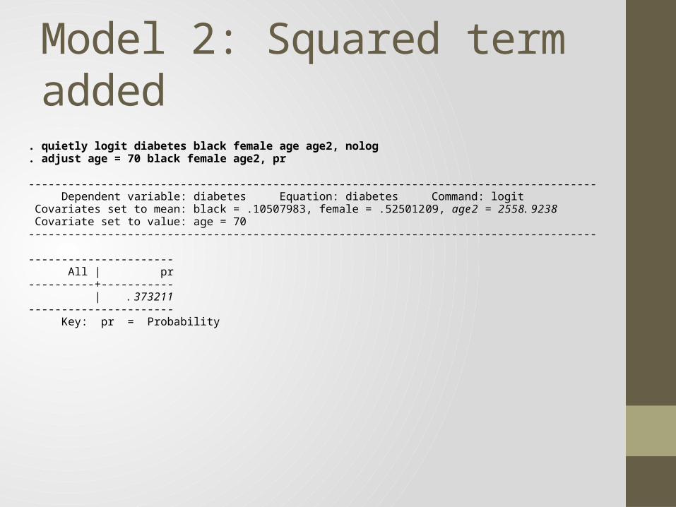
Model 2: Squared term added

. quietly logit diabetes black female age age2, nolog

. adjust age = 70 black female age2, pr -------------------------------------------------------------------------------------- Dependent variable: diabetes Equation: diabetes Command: logit Covariates set to mean: black = .10507983, female = .52501209, age2 = 2558.9238 Covariate set to value: age = 70 -------------------------------------------------------------------------------------- ---------------------- All | pr ----------+----------- | .373211 ---------------------- Key: pr = Probability

• In this model, adjust reports a much higher predicted probability of diabetes than before – 37 percent as opposed to 11 percent!

• But, luckily, adjust is wrong. Because it does not know that age and age2 are related, it uses the mean value of age2 in its calculations, rather than the correct value of 70 squared.

• While there are ways to fix this, using the margins command and factor variables is a safer solution. • The use of factor variables tells margins that age and age^2 are

not independent of each other and it does the calculations accordingly.

• In this case it leads to a much smaller (and also correct) estimate of 10.3 percent.

. quietly logit diabetes i.black i.female age c.age#c.age, nolog

. margins, at(age = 70) atmeans Adjusted predictions Number of obs = 10335 Model VCE : OIM Expression : Pr(diabetes), predict() at : 0.black = .8949202 (mean) 1.black = .1050798 (mean) 0.female = .4749879 (mean) 1.female = .5250121 (mean) age = 70 ------------------------------------------------------------------------------ | Delta-method | Margin Std. Err. z P>|z| [95% Conf. Interval] -------------+---------------------------------------------------------------- _cons | .1029814 .0063178 16.30 0.000 .0905988 .115364 ------------------------------------------------------------------------------

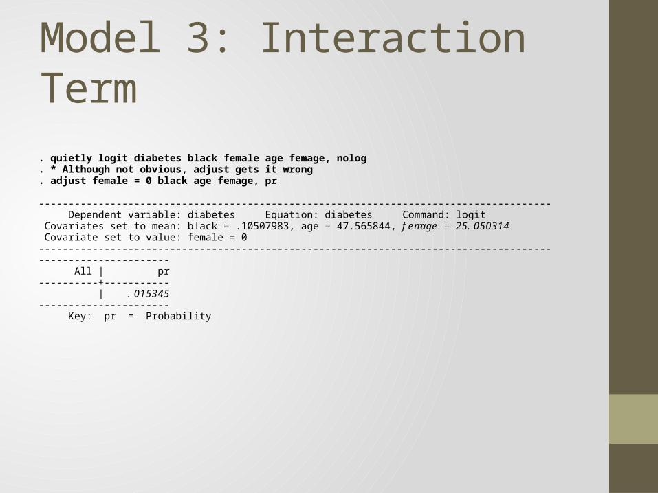
Model 3: Interaction Term

. quietly logit diabetes black female age femage, nolog

. * Although not obvious, adjust gets it wrong

. adjust female = 0 black age femage, pr -------------------------------------------------------------------------------------- Dependent variable: diabetes Equation: diabetes Command: logit Covariates set to mean: black = .10507983, age = 47.565844, femage = 25.050314 Covariate set to value: female = 0 -------------------------------------------------------------------------------------- ---------------------- All | pr ----------+----------- | .015345 ---------------------- Key: pr = Probability

• Once again, adjust gets it wrong

• If female = 0, femage must also equal zero

• But adjust does not know that, so it uses the average value of femage instead.

• Margins does know that the different components of the interaction term are related, and does the calculation right.

. quietly logit diabetes i.black i.female age i.female#c.age, nolog

. margins female, atmeans grand Adjusted predictions Number of obs = 10335 Model VCE : OIM Expression : Pr(diabetes), predict() at : 0.black = .8949202 (mean) 1.black = .1050798 (mean) 0.female = .4749879 (mean) 1.female = .5250121 (mean) age = 47.56584 (mean) ------------------------------------------------------------------------------ | Delta-method | Margin Std. Err. z P>|z| [95% Conf. Interval] -------------+---------------------------------------------------------------- female | 0 | .0250225 .0027872 8.98 0.000 .0195597 .0304854 1 | .0372713 .0029632 12.58 0.000 .0314635 .0430791 | _cons | .0308641 .0020865 14.79 0.000 .0267746 .0349537 ------------------------------------------------------------------------------

Model 4: Multiple dummies

. quietly logit diabetes black female agegrp2 agegrp3 agegrp4 agegrp5 agegrp6

. adjust agegrp6 = 1 black female agegrp2 agegrp3 agegrp4 agegrp5, pr -------------------------------------------------------------------------------------- Dependent variable: diabetes Equation: diabetes Command: logit Covariates set to mean: black = .10507983, female = .52501209, agegrp2 = .15674891, agegrp3 = .12278665, agegrp4 = .12472182, agegrp5 = .27595549 Covariate set to value: agegrp6 = 1 -------------------------------------------------------------------------------------- ---------------------- All | pr ----------+----------- | .320956 ---------------------- Key: pr = Probability

• More depressing news for old people: now adjust says they have a 32 percent chance of having diabetes

• But once again adjust is wrong: If you are in the oldest age group, you can’t also have partial membership in some other age category. 0, not the means, is the correct value to use for the other age variables when computing probabilities.

• Margins realizes this and does it right again.

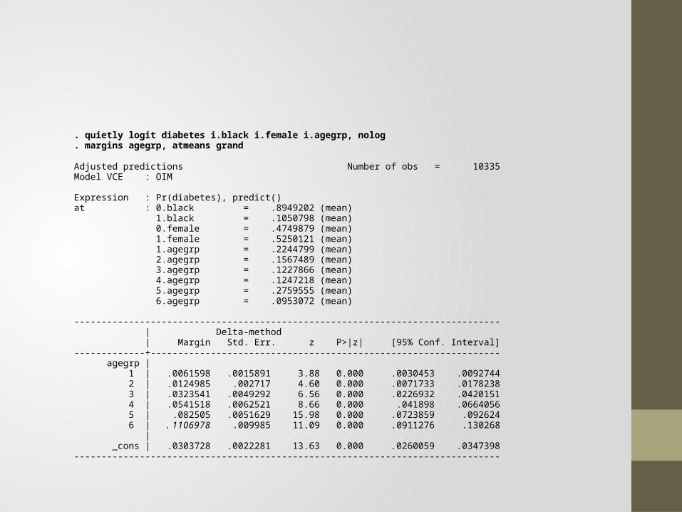
. quietly logit diabetes i.black i.female i.agegrp, nolog

. margins agegrp, atmeans grand Adjusted predictions Number of obs = 10335 Model VCE : OIM Expression : Pr(diabetes), predict() at : 0.black = .8949202 (mean) 1.black = .1050798 (mean) 0.female = .4749879 (mean) 1.female = .5250121 (mean) 1.agegrp = .2244799 (mean) 2.agegrp = .1567489 (mean) 3.agegrp = .1227866 (mean) 4.agegrp = .1247218 (mean) 5.agegrp = .2759555 (mean) 6.agegrp = .0953072 (mean) ------------------------------------------------------------------------------ | Delta-method | Margin Std. Err. z P>|z| [95% Conf. Interval] -------------+---------------------------------------------------------------- agegrp | 1 | .0061598 .0015891 3.88 0.000 .0030453 .0092744 2 | .0124985 .002717 4.60 0.000 .0071733 .0178238 3 | .0323541 .0049292 6.56 0.000 .0226932 .0420151 4 | .0541518 .0062521 8.66 0.000 .041898 .0664056 5 | .082505 .0051629 15.98 0.000 .0723859 .092624 6 | .1106978 .009985 11.09 0.000 .0911276 .130268 | _cons | .0303728 .0022281 13.63 0.000 .0260059 .0347398 ------------------------------------------------------------------------------

Marginal Effects – MEMs, AMEs, & MERs. * Back to basic model . logit diabetes i.black i.female age , nolog Logistic regression Number of obs = 10335 LR chi2(3) = 374.17 Prob > chi2 = 0.0000 Log likelihood = -1811.9828 Pseudo R2 = 0.0936 ------------------------------------------------------------------------------ diabetes | Coef. Std. Err. z P>|z| [95% Conf. Interval] -------------+---------------------------------------------------------------- 1.black | .7179046 .1268061 5.66 0.000 .4693691 .96644 1.female | .1545569 .0942982 1.64 0.101 -.0302642 .3393779 age | .0594654 .0037333 15.93 0.000 .0521484 .0667825 _cons | -6.405437 .2372224 -27.00 0.000 -6.870384 -5.94049 ------------------------------------------------------------------------------

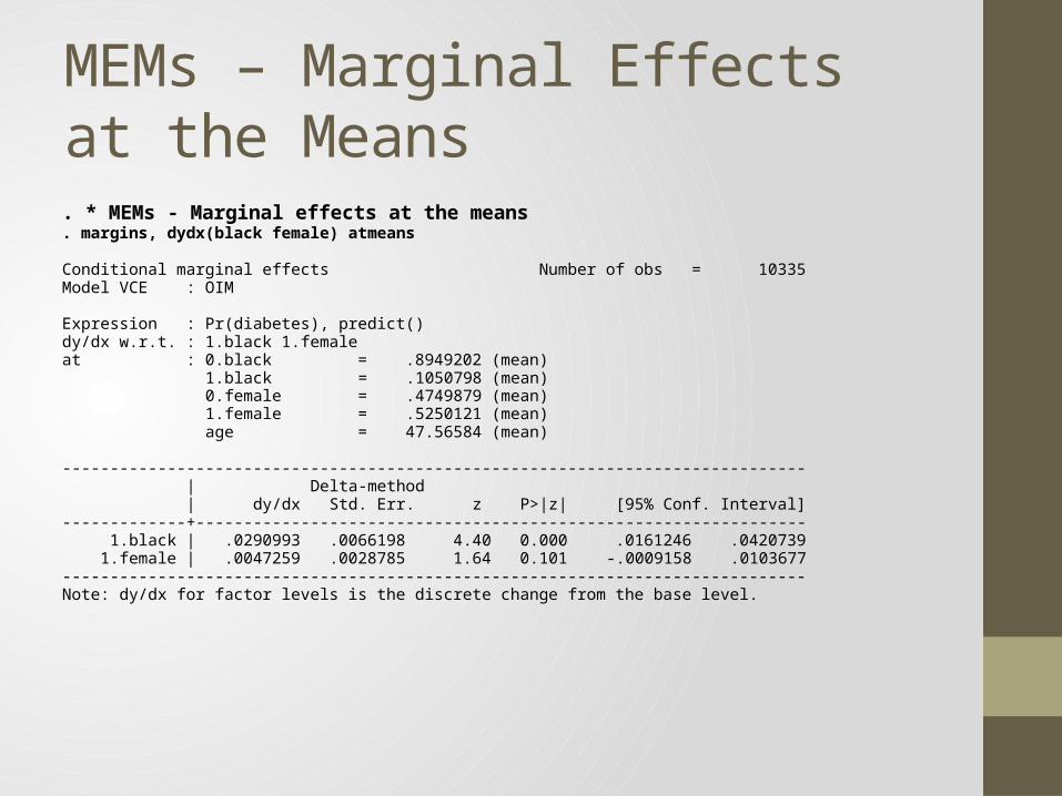
MEMs – Marginal Effects at the Means. * MEMs - Marginal effects at the means . margins, dydx(black female) atmeans Conditional marginal effects Number of obs = 10335 Model VCE : OIM Expression : Pr(diabetes), predict() dy/dx w.r.t. : 1.black 1.female at : 0.black = .8949202 (mean) 1.black = .1050798 (mean) 0.female = .4749879 (mean) 1.female = .5250121 (mean) age = 47.56584 (mean) ------------------------------------------------------------------------------ | Delta-method | dy/dx Std. Err. z P>|z| [95% Conf. Interval] -------------+---------------------------------------------------------------- 1.black | .0290993 .0066198 4.40 0.000 .0161246 .0420739 1.female | .0047259 .0028785 1.64 0.101 -.0009158 .0103677 ------------------------------------------------------------------------------ Note: dy/dx for factor levels is the discrete change from the base level.

• The results tell us that, if you had two otherwise-average individuals, one white, one black, the black’s probability of having diabetes would be 2.9 percent higher.

• And what do we mean by average? With MEMs, average is defined as having the mean value for the other independent variables in the model, i.e. 47.57 years old, 10.5 percent black, and 52.5 percent female.

• MEMs are easy to explain. They have been widely used. Indeed, for a long time, MEMs were the only option with Stata, because that is all the old mfx command supported.

• But, many do not like MEMs. While there are people who are 47.57 years old, there is nobody who is 10.5 percent black or 52.5 percent female.

• Further, the means are only one of many possible sets of values that could be used – and a set of values that no real person could actually have seems troublesome.

• For these and other reasons, many researchers prefer AMEs.

AMEs – Average Marginal Effects

. margins, dydx(black female) Average marginal effects Number of obs = 10335 Model VCE : OIM Expression : Pr(diabetes), predict() dy/dx w.r.t. : 1.black 1.female ------------------------------------------------------------------------------ | Delta-method | dy/dx Std. Err. z P>|z| [95% Conf. Interval] -------------+---------------------------------------------------------------- 1.black | .0400922 .0087055 4.61 0.000 .0230297 .0571547 1.female | .0067987 .0041282 1.65 0.100 -.0012924 .0148898 ------------------------------------------------------------------------------ Note: dy/dx for factor levels is the discrete change from the base level.

• Intuitively, the AME for black is computed as follows:

• Go to the first case. Treat that person as though s/he were white, regardless of what the person’s race actually is. Leave all other independent variable values as is. Compute the probability this person (if he or she were white) would have diabetes

• Now do the same thing, this time treating the person as though they were black.

• The difference in the two probabilities just computed is the marginal effect for that case

• Repeat the process for every case in the sample

• Compute the average of all the marginal effects you have computed. This gives you the AME for black.

• In effect, you are comparing two hypothetical populations – one all white, one all black – that have the exact same values on the other independent variables in the model.

• Since the only difference between these two populations is their race, race must be the cause of the differences in their likelihood of diabetes.

• Many people like the fact that all of the data is being used, not just the means, and feel that this leads to superior estimates.

• Others, however, are not convinced that treating men as though they are women, and women as though they are men, really is a better way of computing marginal effects.

• The biggest problem with both of the last two approaches, however, may be that they only produce a single estimate of the marginal effect. However “average” is defined, averages can obscure difference in effects across cases.

• In reality, the effect that variables like race have on the probability of success varies with the characteristics of the person, e.g. racial differences could be much greater for older people than for younger.

• If we really only want a single number for the effect of race, we might as well just estimate an OLS regression, as OLS coefficients and AMEs are often very similar to each other.

• MERs (Marginal Effects at Representative Values) may therefore often be a superior alternative.

• MERs can be both intuitively meaningful, while showing how the effects of variables vary by other characteristics of the individual.

• With MERs, you choose ranges of values for one or more variables, and then see how the marginal effects differ across that range.

. margins, dydx(black female) at(age=(20 30 40 50 60 70)) vsquish Average marginal effects Number of obs = 10335 Model VCE : OIM Expression : Pr(diabetes), predict() dy/dx w.r.t. : 1.black 1.female 1._at : age = 20 2._at : age = 30 3._at : age = 40 4._at : age = 50 5._at : age = 60 6._at : age = 70 ------------------------------------------------------------------------------ | Delta-method | dy/dx Std. Err. z P>|z| [95% Conf. Interval] -------------+---------------------------------------------------------------- 1.black | _at | 1 | .0060899 .0016303 3.74 0.000 .0028946 .0092852 2 | .0108784 .0027129 4.01 0.000 .0055612 .0161956 3 | .0192101 .0045185 4.25 0.000 .0103541 .0280662 4 | .0332459 .0074944 4.44 0.000 .018557 .0479347 5 | .0555816 .0121843 4.56 0.000 .0317008 .0794625 6 | .0877803 .0187859 4.67 0.000 .0509606 .1245999 -------------+---------------------------------------------------------------- 1.female | _at | 1 | .0009933 .0006215 1.60 0.110 -.0002248 .0022114 2 | .00178 .0010993 1.62 0.105 -.0003746 .0039345 3 | .003161 .0019339 1.63 0.102 -.0006294 .0069514 4 | .0055253 .0033615 1.64 0.100 -.001063 .0121137 5 | .0093981 .0057063 1.65 0.100 -.001786 .0205821 6 | .0152754 .0092827 1.65 0.100 -.0029184 .0334692 ------------------------------------------------------------------------------ Note: dy/dx for factor levels is the discrete change from the base level.

• Earlier, the AME for black was 4 percent.

• But, when we estimate marginal effects for different ages, we see that the effect of black differs greatly by age. It is less than 1 percent for 20 year olds and almost 9 percent for those aged 70.

• Similarly, while the AME for gender was only 0.6 percent, at different ages the effect is much smaller or much higher than that.

• In a large model, it may be cumbersome to specify representative values for every variable, but you can do so for those of greatest interest.