Using Synthetic Adjustments and Controlling to Improve ...

Vol.:(0123456789)

Population Research and Policy Review (2021) 40:1355–1383https://doi.org/10.1007/s11113-021-09646-7

1 3

ORIGINAL RESEARCH

Using Synthetic Adjustments and Controlling to Improve County Population Forecasts from the Hamilton–Perry Method

Jeff Tayman1 · David A. Swanson2,3 · Jack Baker4

Published online: 22 March 2021 © The Author(s) 2021

AbstractTayman and Swanson (J Popul Res 34(3):209–231, 2017) found in Washington State counties that a forecast based on the Hamilton–Perry method using a synthetic adjustment (SYN) of cohort change ratios and child-woman ratios had greater accu-racy and less bias compared to forecasts holding these ratios constant (CONST). In this paper, we assess the robustness of SYN’s efficacy by evaluating forecast accu-racy, bias, and distributional error across age groups in counties nationwide. We also investigate whether forecast errors and their patterns change for SYN and CONST if forecasts by age and gender are adjusted to an independent total population forecast for each county. Our main findings are as follows: (1) SYN lowers forecast error compared to CONST whether the forecasts are controlled or not; (2) controlling also leads to the improvements in forecast error, often exceeding those in SYN; and (3) using SYN and controlling together has the greatest effect in reducing forecast error. These findings remain after controlling for population size and growth rate, but the positive impacts on forecast error of SYN and controlling are most evident in coun-ties with less than 30,000 population and that grow by 15% or more.

Keywords Hamilton–Perry method · Synthetic adjustment · Forecast evaluation

* Jeff Tayman [email protected]

1 Department of Economics, University of California San Diego, La Jolla, CA 92093, USA2 Department of Sociology, University of California Riverside, Riverside, CA 92521, USA3 Center for Studies in Demography and Ecology, University of Washington, Seattle, WA 98195,

USA4 Transamerica Life, Underwriting Modernization – Research & Development, Cedar Rapids,

IA 52404, USA

http://crossmark.crossref.org/dialog/?doi=10.1007/s11113-021-09646-7&domain=pdf

1356 J. Tayman et al.

1 3

Introduction

Although the general idea of a cohort change ratio (CCR) has been around for at least 100 years (Hardy and Wyatt 1911) and it has been widely used to generate population forecasts since their “re-introduction” by Hamilton and Perry (1962), CCRs have largely remained a tool of applied demographers who generate pop-ulation forecasts (Smith et al. 2013, pp. 176–179). The Hamilton–Perry (H–P) method is a short-cut variant of the cohort-component method (CCM) that has much smaller data requirements than its more data-intensive cousin, while still providing forecasts of the population by age and gender (as well race, ethnicity, or other characteristics, if so desired). Instead of specific rates for each compo-nent of population change, as used in the CCM, H–P method forecasts for all but the youngest age groups are based on CCRs that combine the effects of mortal-ity and migration. Child-woman ratios (CWR) are used to forecast the youngest age groups. CCRs and CWRs are most often obtained from the two most recent censuses, but they can be based on age distributions from any two points in time.

Consequently, the H–P method requires much less time and resources to implement than the CCM. Not surprisingly, it has mainly been used for subcounty geographic areas where fertility, mortality, and migration data are non-existent, unreliable, or difficult to obtain (Baker et al. 2014; Smith et al. 2013, p. 176; Swanson et al. 2010). This method has also gained acceptance as research has demonstrated its practical value and reasonable error levels in forecasting popula-tions (Baker et al. 2017, Chapter 4; Kodiko 2014; Smith and Shahidullah 1995; Smith and Tayman 2003; Swanson and Tayman 2017). Although the H–P method has been primarily used for subcounty geographic areas, its minimal data require-ments combined with the ability to forecast age and other characteristics make it attractive for use at higher levels of geography such as states and counties when information about the components of population change is not needed (Hauer 2019; Rayer and Wang 2020).

Assessments of the H–P method have been based on the usual assumption that the CCRs developed over the base period and CWRs developed for the launch year are held constant over the forecast horizon (horizon) (CONST). Smith et al. (2013, p. 179) discuss the possibility of relaxing this assumption by averaging CCRs and CWRs from several recent censuses (AVG), by extrapolating histori-cal trends in these ratios (TREND), or by using a synthetic approach based on CCR and CWR forecasts from a population in a larger geographic area (SYN). AVG and TREND make individual adjustments to the CCRs and CWRs for each area being forecast. SYN, used frequently and successfully in state and local fore-casting (Smith et al. 2013, p. 65; Williamson 2013), does not make area-specific adjustments, but applies the same proportionate change to each area based on a forecast for a larger geographic area (i.e., state changes applied to each county). SYN globally incorporates information from the horizon being forecast, while AVG and TREND rely solely on geographic-specific historical patterns.

Tayman and Swanson (2017) evaluated these approaches for modifying CCRs and CWRs for Washington State counties and compared their forecast errors to

1357

1 3

Using Synthetic Adjustments and Controlling to Improve County…

errors from CONST. They evaluated 10-year forecasts using a 2000 launch year and a 2010 horizon year, historical data from 1980 to 2000 for each county, and state-level CCRs and CWRs from 2000 and 2010. They found that (1) forecasts based on the CONST were almost universally better (lower error) than forecasts based on TREND; (2) AVG fared much better against CONST; its forecasts, gen-erally had less bias and greater accuracy; (3) SYN outperformed forecasts from TREND and CONST (less bias, greater accuracy, and less allocation error); and (4) SYN also outperformed AVG, but to a lesser extent compared with TREND and CONST. These findings suggested there is more to be gained in the H–P method by applying a global adjustment covering the horizon rather than basing adjustments on area-specific historical changes.

This paper extends Tayman and Swanson (2017) in two fundamental ways. First, Washington State is a high growth state and its counties lacked variation in growth rates, which are almost always positive. We assess the robustness of the efficacy of SYN by evaluating forecast accuracy, bias, and distributional error in counties nationwide. Before this study, evaluations of the H–P method usually focused on counties in a single state. Second, their study only examined uncontrolled H–P fore-casts. It is advisable to control H–P forecasts by age and gender to independent fore-casts of the total population (Baker et al. 2020; Smith et al. 2013, p. 181; Swanson et al. 2010). Such “controlling” is common when forecasting or estimating the popu-lations of substate areas such as counties (Pittenger 1976, pp. 80–89; Smith et al. 2013, pp. 258–272; Swanson and Tayman 2012, pp. 254–265). We examine whether forecast errors and their patterns change for SYN and CONST by comparing uncon-trolled H–P forecasts with H–P forecasts adjusted to an independent total population forecast for each county. We also offer suggestions and guidelines for implementing the H–P method in county-level forecasts.

Methodology

Hamilton–Perry Method Alternatives

The H–P method uses CCRs, which are calculated by dividing the population age x in year t by the population age x–10 in year t–10. CCRs are usually calculated sepa-rately for males and females. These CCRs are applied to each age/gender group in year t to provide forecasts by age in the year t + 10. Given the nature of the CCRs, 10–14 is the youngest 5-year age group for which forecasts can be made if there are 10 years between censuses. Children younger than age 10 are forecast using CWRs from the launch year (i.e., males or females 0–4/females ages 15–44 and males or females ages 5–9/females ages 20–49). Equations 1 through 3 represent the usual application of the H–P method (i.e., holding CCRs and CWRs from the most recent 10-year period constant over the horizon):

(1)nPx+10,g,t+10 = nCCRx,g,t × nPx,g,t (Ages 10+),


1 3

where n is the width of the age group, x is the beginning of the age group, g is gen-der, t is the launch year, P is the population, CCR is the cohort change ratio, CWR is the child-woman ratio, and FP is the female population.

H–P forecasts using SYN are computed by (bold indicates the state):

where SYNCCR is the age-specific CCR adjustment for the state, and SYNCWR is the age-specific CWR adjustment for the state.

Total Population Controls

An independent forecast of the 2010 total population for each county is needed to create the controlled forecast alternatives for CONST and SYN. The base period for these forecasts is 1990–2000. Controlling is accomplished by applying a county-specific proportionate adjustment to the initial age and gender-specific forecasts so they add to the independent county total population forecast. The adjustment factor is the total population forecast obtained by summing the age and gender forecast divided by the independent total population forecast.

An average of five extrapolation methods is used to construct the independent total population forecast. The first method holds the population constant at its 2000 level. The second method assumes the population from 2000 to 2010 changes at the same numeric amount as it did during the base period (1990–2000). The third method assumes the population from 2000 to 2010 changes at the same percentage amount as it did during the base period. The fourth method assumes the change in the share of the county to the state population in the base period is the same between 2000 and 2010. The final method assumes that the county’s share of the state’s pop-ulation change during the base period will be the same between 2000 and 2010. A detailed discussion of these methods is found in Smith et al. (2013, Chapter 8).

(2)4P0,g,t+10 = 4CWR0,g,t × 44FP15,t+10 (Ages 0 − 4),

(3)9P5,g,t+10 = 9CWR5,g,t × 49FP20,t+10 (Ages 5 − 9),

(4)��n��x,g =(

n��x,g,t+��

/

n��x,g,t

)

,

(5)��

�,g =(

��

�,g,t+��

/

��

�,g,t

)

,

(6)��

�,g =(

��

�,g,t+��

/

��

�,g,t

)

,

(7)nPx+10,g,t+10 =(

nCCRx,g,t × ��n��x,g

)

×n Px,g,t(Ages 10+),

(8)4P0,g,t+10 =(

4CWR0,g,t × ��

�,g

)

×44 FP15,t+10(Ages 0 − 4),

(9)9P5,g,t+10 =(

9CWR5,g,t × ��

�,g

)

×49 FP20,t+10(Ages 5 − 9),

1359

1 3


Forecast Error Measures

We analyze several commonly used measures that capture three dimensions of forecast error—accuracy, bias, and allocation error (Swanson 2015; Swanson et al. 2011). Error is defined as the difference between the simulated forecast and census count. The mean algebraic percent error (MALPE) measures bias in which positive and negative values offset each other. A positive MALPE reflects the tendency for the forecasts to be too high on average and a negative MALPE reflect the tendency for the forecasts to be too low on average. The mean absolute percent error (MAPE) measures forecast accuracy in which positive and negative errors do not offset each other. It shows the average percentage difference between the forecast and observed population, ignoring the sign of the error.1

The MAPE and MALPE are based on forecast errors for a particular geographic area. Another perspective views the misallocation of the forecast across geographic space or a given variable, such as age. Our focus here is not on geographic misallo-cation, but on the accuracy of the age distribution forecast. The Index of Dissimilar-ity (IOD) is widely used to measure allocation error (Duncan et al. 1961; Fonseca and Tayman 1989; Massey and Denton 1988). The IOD compares the percentage distribution of the forecast population by age group and the corresponding percent-age distribution in the census. The IOD calculates the percentage that the forecast distribution would have to change to match the census distribution. The IOD ranges from 0 to 100%, with 0 indicating identical percentage distributions and 100 indicat-ing a complete disparity between the forecast and census age distributions.

Data

Out of a universe of 3140 counties in the U.S, our data consist of 3106 counties or county equivalents whose geographic boundaries remained constant from 1990 to 2010.2 These counties contain approximately 99% of the counties and the total pop-ulation in the U.S. We collected 1990, 2000, and 2010 census data for 18 5-year age groups (0–4, 5–9…., 80–84, and 85 years and older) for males and females. Aside from boundary changes, implementing the H–P method is impacted by zero popu-lation counts. A CCR is undefined if the earlier census count (the denominator) is zero. At the county level of geography zero population counts are much less of a problem than for subcounty areas such as census tracts. We encountered only 68

1 The error distribution underlying the MAPE is often asymmetrical and right skewed, causing the MAPE to overstate the error represented by most of the observations. MAPE-R and the median absolute percent error (MEDAPE) are two measures of accuracy that have been used when the error distribu-tion underlying the MAPE is highly asymmetrical (Baker et al. 2020; Swanson et al. 2011, 2012). Since forecast errors are generally stable across a variety of error measures (Rayer 2007), we forego using MEDAPE and MAPE-R in this study.2 The 34 excluded areas are: 1) all 27 boroughs in Alaska; 2) Adams, Boulder, Broomfield, Jefferson, and Weld counties in Colorado; and 3) Alleghany and Halifax counties in Virginia.


1 3

zero cells in the age and gender data for all three census points and assigned them a value of 1.

We constructed H–P forecasts for four alternatives: (1) UNCONST (holding CCRs and CWRs constant), uncontrolled, (2) CTRLCONST, CONST controlled to an independent total county population forecast; (3) UNSYN (county CCRs and CWRs adjusted by state trends in CCRs and CWRs), uncontrolled; and (4) CTRL-SYN, SYN controlled. We prepared 10-year forecasts using the 2000 launch year and 2010 horizon year. CONST and SYN used CCRs from the 1990–2000 decade and CWRs from 2000. SYN also required state-level CCRs from 1990 to 2000 and 2000–2010 and state-level CWRs for 2000 and 2010. The decennial censuses pro-vide the state-level CCRS and CWRs for 1990 and 2000. To represent an actual forecasting situation, we used 2010 state forecasts by age and gender released by the U.S. Census Bureau in 2005 obtained from the Center for Disease Control’s WON-DER data platform (https:// wonder. cdc. gov/ popul ation- proje ctions. html). For each alternative, a forecast was prepared for the 18 age groups and by gender.

Analysis

Total Population Forecast Error3

For the analysis, we treat the UNCONST forecast as the baseline alternative that the other alternatives are compared to. This strategy provides a clearer focus on the efficacy of controlling and SYN relative to the most common application of the H–P method.

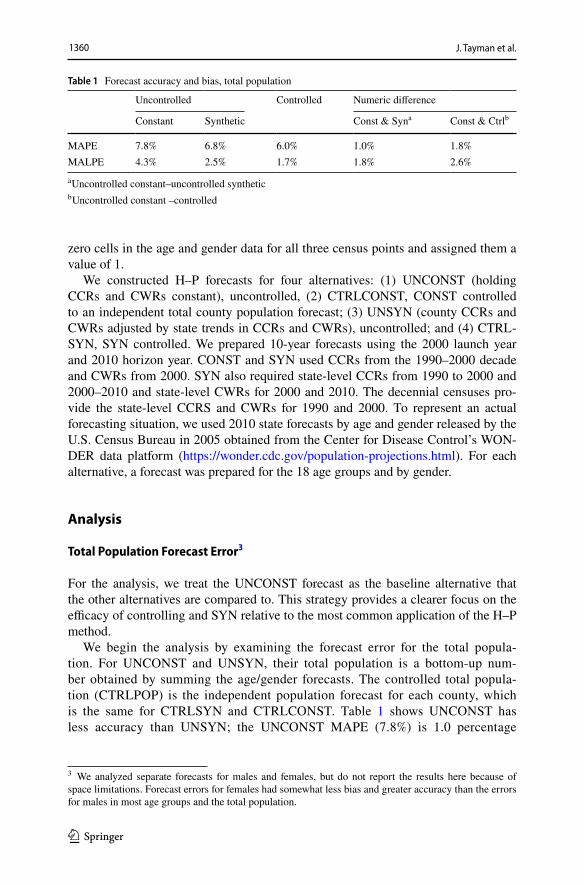
We begin the analysis by examining the forecast error for the total popula-tion. For UNCONST and UNSYN, their total population is a bottom-up num-ber obtained by summing the age/gender forecasts. The controlled total popula-tion (CTRLPOP) is the independent population forecast for each county, which is the same for CTRLSYN and CTRLCONST. Table 1 shows UNCONST has less accuracy than UNSYN; the UNCONST MAPE (7.8%) is 1.0 percentage

Table 1 Forecast accuracy and bias, total population

a Uncontrolled constant–uncontrolled syntheticb Uncontrolled constant –controlled

Uncontrolled Controlled Numeric difference

Constant Synthetic Const & Syna Const & Ctrlb

MAPE 7.8% 6.8% 6.0% 1.0% 1.8%MALPE 4.3% 2.5% 1.7% 1.8% 2.6%

3 We analyzed separate forecasts for males and females, but do not report the results here because of space limitations. Forecast errors for females had somewhat less bias and greater accuracy than the errors for males in most age groups and the total population.

https://wonder.cdc.gov/population-projections.html

1361

1 3


point higher than the UNSYN MAPE. CTRLPOP is the most accurate alterna-

tive; the UNCONST MAPE is 1.8 percentage points higher than the CTRLPOP MAPE. The total population forecast is biased upwards in all three alternatives with MALPE’s ranging from 1.7% for CTRLPOP to 2.5% for UNSYN and 4.3% for UNCONST. The UNCONST MALPE is 1.8 percentage points higher than the UNSYN MALPE and 2.6 percentage points higher than the CTRLPOP MALPE.

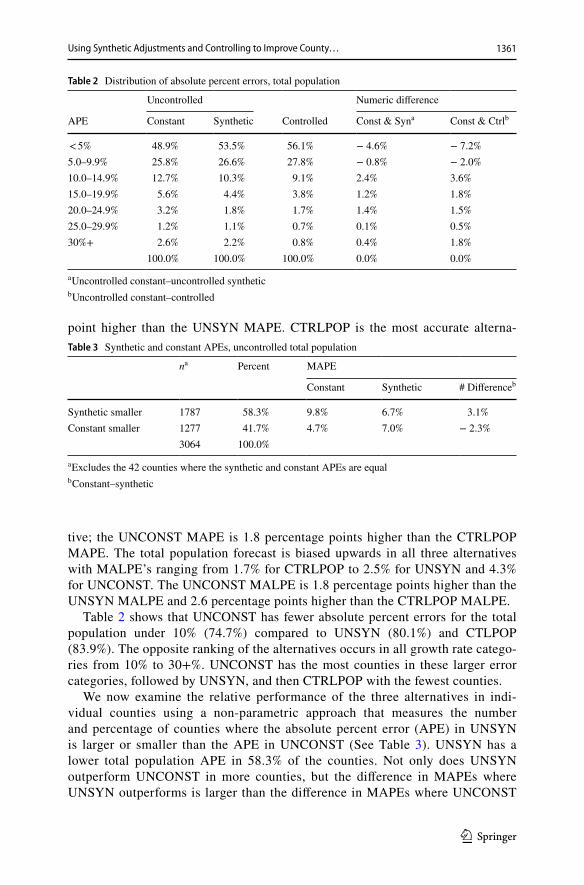
Table 2 shows that UNCONST has fewer absolute percent errors for the total population under 10% (74.7%) compared to UNSYN (80.1%) and CTLPOP (83.9%). The opposite ranking of the alternatives occurs in all growth rate catego-ries from 10% to 30+%. UNCONST has the most counties in these larger error categories, followed by UNSYN, and then CTRLPOP with the fewest counties.

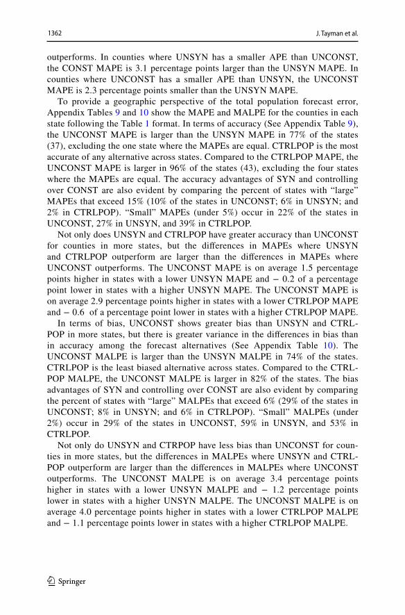
We now examine the relative performance of the three alternatives in indi-vidual counties using a non-parametric approach that measures the number and percentage of counties where the absolute percent error (APE) in UNSYN is larger or smaller than the APE in UNCONST (See Table 3). UNSYN has a lower total population APE in 58.3% of the counties. Not only does UNSYN outperform UNCONST in more counties, but the difference in MAPEs where UNSYN outperforms is larger than the difference in MAPEs where UNCONST

Table 2 Distribution of absolute percent errors, total population

a Uncontrolled constant–uncontrolled syntheticb Uncontrolled constant–controlled

Uncontrolled Numeric difference

APE Constant Synthetic Controlled Const & Syna Const & Ctrlb

< 5% 48.9% 53.5% 56.1% − 4.6% − 7.2%5.0–9.9% 25.8% 26.6% 27.8% − 0.8% − 2.0%10.0–14.9% 12.7% 10.3% 9.1% 2.4% 3.6%15.0–19.9% 5.6% 4.4% 3.8% 1.2% 1.8%20.0–24.9% 3.2% 1.8% 1.7% 1.4% 1.5%25.0–29.9% 1.2% 1.1% 0.7% 0.1% 0.5%30%+ 2.6% 2.2% 0.8% 0.4% 1.8%

100.0% 100.0% 100.0% 0.0% 0.0%

Table 3 Synthetic and constant APEs, uncontrolled total population

a Excludes the 42 counties where the synthetic and constant APEs are equalb Constant–synthetic

na Percent MAPE

Constant Synthetic # Differenceb

Synthetic smaller 1787 58.3% 9.8% 6.7% 3.1%Constant smaller 1277 41.7% 4.7% 7.0% − 2.3%

3064 100.0%


1 3

outperforms. In counties where UNSYN has a smaller APE than UNCONST, the CONST MAPE is 3.1 percentage points larger than the UNSYN MAPE. In counties where UNCONST has a smaller APE than UNSYN, the UNCONST MAPE is 2.3 percentage points smaller than the UNSYN MAPE.

To provide a geographic perspective of the total population forecast error, Appendix Tables 9 and 10 show the MAPE and MALPE for the counties in each state following the Table 1 format. In terms of accuracy (See Appendix Table 9), the UNCONST MAPE is larger than the UNSYN MAPE in 77% of the states (37), excluding the one state where the MAPEs are equal. CTRLPOP is the most accurate of any alternative across states. Compared to the CTRLPOP MAPE, the UNCONST MAPE is larger in 96% of the states (43), excluding the four states where the MAPEs are equal. The accuracy advantages of SYN and controlling over CONST are also evident by comparing the percent of states with “large” MAPEs that exceed 15% (10% of the states in UNCONST; 6% in UNSYN; and 2% in CTRLPOP). “Small” MAPEs (under 5%) occur in 22% of the states in UNCONST, 27% in UNSYN, and 39% in CTRLPOP.

Not only does UNSYN and CTRLPOP have greater accuracy than UNCONST for counties in more states, but the differences in MAPEs where UNSYN and CTRLPOP outperform are larger than the differences in MAPEs where UNCONST outperforms. The UNCONST MAPE is on average 1.5 percentage points higher in states with a lower UNSYN MAPE and − 0.2 of a percentage point lower in states with a higher UNSYN MAPE. The UNCONST MAPE is on average 2.9 percentage points higher in states with a lower CTRLPOP MAPE and − 0.6 of a percentage point lower in states with a higher CTRLPOP MAPE.

In terms of bias, UNCONST shows greater bias than UNSYN and CTRL-POP in more states, but there is greater variance in the differences in bias than in accuracy among the forecast alternatives (See Appendix Table 10). The UNCONST MALPE is larger than the UNSYN MALPE in 74% of the states. CTRLPOP is the least biased alternative across states. Compared to the CTRL-POP MALPE, the UNCONST MALPE is larger in 82% of the states. The bias advantages of SYN and controlling over CONST are also evident by comparing the percent of states with “large” MALPEs that exceed 6% (29% of the states in UNCONST; 8% in UNSYN; and 6% in CTRLPOP). “Small” MALPEs (under 2%) occur in 29% of the states in UNCONST, 59% in UNSYN, and 53% in CTRLPOP.

Not only do UNSYN and CTRPOP have less bias than UNCONST for coun-ties in more states, but the differences in MALPEs where UNSYN and CTRL-POP outperform are larger than the differences in MALPEs where UNCONST outperforms. The UNCONST MALPE is on average 3.4 percentage points higher in states with a lower UNSYN MALPE and − 1.2 percentage points lower in states with a higher UNSYN MALPE. The UNCONST MALPE is on average 4.0 percentage points higher in states with a lower CTRLPOP MALPE and − 1.1 percentage points lower in states with a higher CTRLPOP MALPE.

1363

1 3


Forecast Error by Age Group

We constructed the forecasts using 17 5-year age groups and a terminal age group of 85 years and older, but evaluate forecast errors using a reduced set of seven groups. These groups cover the full age spectrum, adequately capture the age-specific per-formance of the alternatives, and make the analysis easier to follow. The seven age groups are younger than age 10 (hereafter < 10), 10–19, 20–34, 35–54, 55–64, 65–74, and 75 years and older (hereafter 75+). As a composite measure of the age group accuracy and bias, we also compute the average of the MAPEs and MALPEs across age groups.

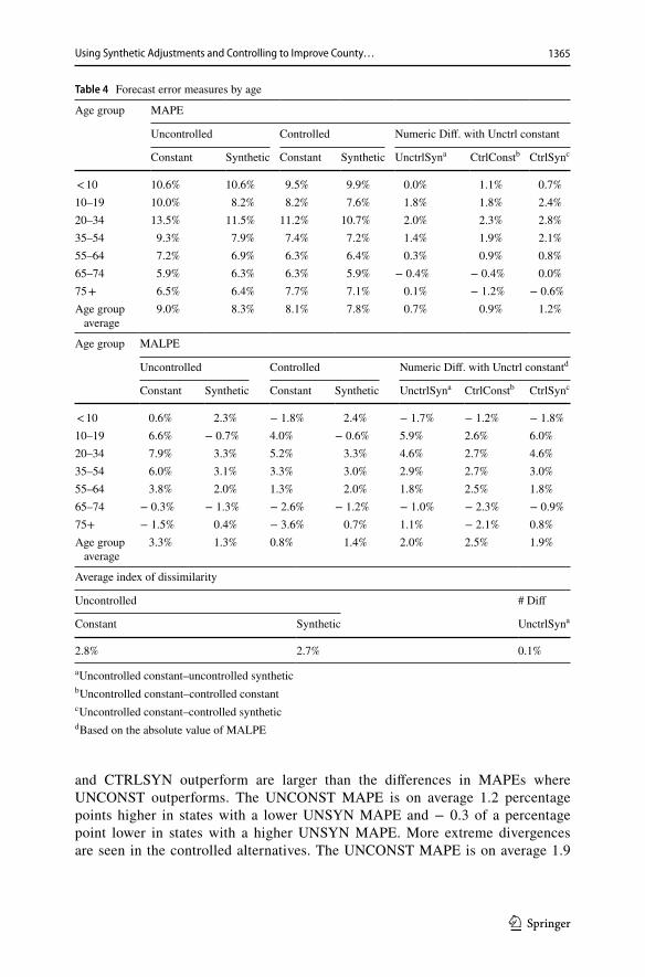
For most age groups, UNCONST is less accurate than the other three forecast alternatives. (See Table 4). UNCONST has a higher MAPE than UNSYN in every age group and the age group average, except for ages 65–74 where the MAPEs are − 0.4 of a percentage point apart and ages under 10 where the MAPEs are equal. Simi-lar patterns are seen in both controlled alternatives. UNCONST has a higher MAPE than CTRLCONST in every age group and the age group average, except for ages 65–74 where the MAPEs are − 0.4 of a percentage point apart and ages 75+ where the MAPEs are − 1.2 percentage points apart. The joint application of controlling and SYN (CTRLSYN) produces the most accurate forecasts by age group and the age group average. UNCONST has a higher MAPE than CTRLSYN in every age group and the age group average, except for ages 65–74 where the MAPEs are equal and ages 75+ where the MAPEs are − 0.6 of a percentage point apart. In general, the greatest benefit in terms of accuracy from SYN and controlling is seen in ages 10–54, which are typically most impacted by migration.

The patterns of forecast bias by age group are like those seen for forecast accu-racy but the improvements in bias compared to UNCONST are somewhat larger. UNCONST has a higher MALPE than UNSYN in every age group and the age group average, except for ages 65–74 where the MAPEs are − 1.0 percentage point apart and ages under 10 where the MAPEs are − 1.7 percentage points apart. Similar patterns are seen in both controlled alternatives. UNCONST has a higher MALPE than CTRLCONST in every age group and the age group average, except for ages 65+ where the MALPEs are just over − 2.0 percentage points apart and ages < 10 where the MALPEs are − 1.2 percentage points apart. UNCONST has a higher MALPE than CTRLSYN in every age group and the age group average, except for ages 65–74 where the MALPEs are − 0.9 of a percentage point apart and ages < 10 where the MAPLEs are − 1.8 percentage points apart. The allocation error across age groups, as measured by the Index of Dissimilarity (IOD), is small and differs by only 0.1 of a percentage point between UNCONST and UNSYN.4

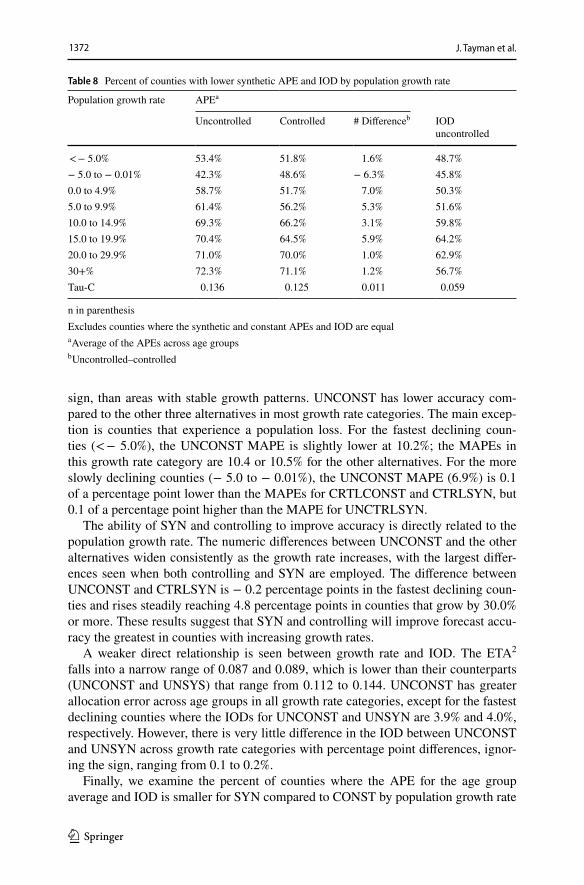
Our last metric looks at the percentage of counties where the APE by age group and age group average is smaller for SYN compared to CONST for both the con-trolled and uncontrolled alternatives and the uncontrolled IOD. As Fig. 1 shows,

4 We only present the uncontrolled alternatives for the IOD. Because we use a single factor for each county to adjust the population by age to the independent total population total, the uncontrolled propor-tionate age distribution will not be affected by this adjustment.


1 3

the percentage is 50.0% or more in all but two comparisons (controlled ages 55–64 (48%) and uncontrolled ages 65–74 (42%) and it varies by age group. Excluding these two age groups, the percentage ranges from 51% for ages < 10 in the controlled alternative to 65% for ages 35–54 in the uncontrolled alternative. These percentages tend to be the highest for ages 10 to 54, the age group average, and the IOD and low-est in ages < 10 and 55–74.

To provide a geographic perspective of the forecast error for age groups, Appen-dix Table 11 shows the MAPE based on the average of the APEs across age groups for the counties in each state following Table 4 format. For most states, UNCONST has lower accuracy in its forecast by age than the other three alternatives. The UNCONST MAPE is larger than the UNSYN MAPE in 75% of the states, exclud-ing the one state where the MAPEs are equal. The lower accuracy of UNCONST is more evident in the controlled alternatives. The UNCONST MAPE is larger than the CTRLCONST MAPE in 82% of the states and 86% of the states in CTRL-SYN. The accuracy disadvantage of UNCONST in forecasting age groups is also evident by comparing the percent of states with “large” MAPEs that exceed 15%. In UNCONST 11% percent of the states have large MAPEs compared to 6% for UNSYN and 4% for CTLRSYN. Only 2% of the states have large errors in CTRL-SYN. “Small” MAPEs (under 7.5%) occur in 33% of the states in UNCONST, the smallest percentage of any alternative. The percentage of “small” MAPEs ranges from 49% in CTRLCONST to 57% in CTRLSYN.

Not only does UNCONST have less accurate forecasts by age than the three other alternatives, but the differences in MAPEs where UNSYN, CTRLCONST,

a Excludes counties where the SYN and CONST APEs are equal.

0.0%

10.0%

20.0%

30.0%

40.0%

50.0%

60.0%

70.0%

<10 10-19 20-34 35-54 55-64 65-74 75+ Average IOD

Uncontrolled

Controlled

Fig. 1 Percentage of counties with lower synthetic APEa

1365

1 3


and CTRLSYN outperform are larger than the differences in MAPEs where UNCONST outperforms. The UNCONST MAPE is on average 1.2 percentage points higher in states with a lower UNSYN MAPE and − 0.3 of a percentage point lower in states with a higher UNSYN MAPE. More extreme divergences are seen in the controlled alternatives. The UNCONST MAPE is on average 1.9

Table 4 Forecast error measures by age

a Uncontrolled constant–uncontrolled syntheticb Uncontrolled constant–controlled constantc Uncontrolled constant–controlled syntheticd Based on the absolute value of MALPE

Age group MAPE

Uncontrolled Controlled Numeric Diff. with Unctrl constant

Constant Synthetic Constant Synthetic UnctrlSyna CtrlConstb CtrlSync

< 10 10.6% 10.6% 9.5% 9.9% 0.0% 1.1% 0.7%10–19 10.0% 8.2% 8.2% 7.6% 1.8% 1.8% 2.4%20–34 13.5% 11.5% 11.2% 10.7% 2.0% 2.3% 2.8%35–54 9.3% 7.9% 7.4% 7.2% 1.4% 1.9% 2.1%55–64 7.2% 6.9% 6.3% 6.4% 0.3% 0.9% 0.8%65–74 5.9% 6.3% 6.3% 5.9% − 0.4% − 0.4% 0.0%75 + 6.5% 6.4% 7.7% 7.1% 0.1% − 1.2% − 0.6%Age group

average9.0% 8.3% 8.1% 7.8% 0.7% 0.9% 1.2%

Age group MALPE

Uncontrolled Controlled Numeric Diff. with Unctrl constantd


< 10 0.6% 2.3% − 1.8% 2.4% − 1.7% − 1.2% − 1.8%10–19 6.6% − 0.7% 4.0% − 0.6% 5.9% 2.6% 6.0%20–34 7.9% 3.3% 5.2% 3.3% 4.6% 2.7% 4.6%35–54 6.0% 3.1% 3.3% 3.0% 2.9% 2.7% 3.0%55–64 3.8% 2.0% 1.3% 2.0% 1.8% 2.5% 1.8%65–74 − 0.3% − 1.3% − 2.6% − 1.2% − 1.0% − 2.3% − 0.9%75+ − 1.5% 0.4% − 3.6% 0.7% 1.1% − 2.1% 0.8%Age group

average3.3% 1.3% 0.8% 1.4% 2.0% 2.5% 1.9%

Average index of dissimilarity

Uncontrolled # Diff

Constant Synthetic UnctrlSyna

2.8% 2.7% 0.1%


1 3

percentage points higher in states with a lower CTRLCONST MAPE and − 0.3 of a percentage point lower in states with a higher CTRLCONST MAPE, and the UNCONST MAPE is on average 2.1 percentage points higher in states with a lower CTRLSYN MAPE and − 0.3 of a percentage point lower in states with a higher CTRLSYN MAPE.

Forecast Error by Population Size and Growth Rate

Population Size

In this section, we analyze the error for the average of the APEs across the seven age groups and the IOD by population size and growth rate. Size represents the population in 2000 and the growth rate represents the percentage change from 1990 to 2000. This investigation examines the MAPE and IOD by size and growth rate categories for SYN and CONST under the uncontrolled and controlled alternatives, again using UNCONST as the basis for comparison.

All four alternatives exhibit the well-known direct relationship between popu-lation size and forecast accuracy (Tayman et al. 2011). As shown in Table 5, this direct relationship is not linear but tends to weaken or disappear once a certain size threshold is reached. UNCONST has lower accuracy, as measured by the MAPE, in most size categories compared to the other three alternatives. The main excep-tion is for counties with 100,000–250,000 persons where the UNCONST MAPE is slightly lower at 5.6%; the MAPEs in this size category range from 5.7 to 5.9% in the other alternatives. The ability of SYN and controlling to improve accuracy is directly related to population size. While the percentage point differences between UNCONST and the other alternatives do not vary greatly by population size, the largest differences are seen in counties under 30,000 persons and range from 0.9 percentage points to 1.9 percentage points. For counties with 30,000 or more people the percent point differences, excluding signs, range from 0.0 percentage points to 0.7 percentage points. These results suggest that SYN and controlling are more use-ful at improving forecast accuracy for counties with less than 30,000 persons, which represent 59% of the counties in this study.

A stronger direct relationship is seen between population size and IOD. The ETA2 falls into a narrow range of 0.215–0.235, which is higher than their counterparts (UNCONST and UNSYN) that range from 0.132 to 0.137.5 However, there is very little difference in the IODs between UNCONST and UNSYN across size categories with percentage point differences, ignoring the sign, ranging from 0.0 to 0.2%.

Finally, we examine the percent of counties where the APE for the age group average and the uncontrolled IOD is smaller for SYN compared to CONST by popu-lation size category. As Table 6 shows, the percentages are 50% or more for every population size category, except for populations between 100,000 and 250,000 in

5 Eta2, commonly used in ANOVA and t test designs, measures the strength of a relationship computed as the ratio of variance in an outcome variable explained by a predictor variable. Its values can range from − 1 to 1.

1367

1 3


Tabl

e 5

Abs

olut

e pe

rcen

t for

ecas

t err

or m

easu

res b

y po

pula

tion

size

Popu

latio

n si

zeM

APE

a

Unc

ontro

lled

Con

trolle

dN

umer

ic D

iff. w

ith U

nctrl

con

stan

t

Con

stan

tSy

nthe

ticC

onst

ant

Synt

hetic

Unc

trlSy

nbC

trlC

onstc

Ctrl

Synd

< 50

00 (2

91)

16.1

%15

.2%

14.5

%14

.3%

0.9%

1.6%

1.8%

d500

0–99

99 (4

45)

11.3

%10

.2%

9.9%

9.6%

1.1%

1.4%

1.7%

10,0

00–1

4,99

9 (3

95)

10.3

%9.

2%8.

6%8.

4%1.

1%1.

7%1.

9%15

,000

–19,

999

(308

)9.

0%8.

0%7.

7%7.

4%1.

0%1.

3%1.

6%20

,000

–29,

999

(381

)8.

1%7.

1%6.

9%6.

6%1.

0%1.

2%1.

5%30

,000

–49,

999

(451

)6.

9%6.

4%6.

4%6.

2%0.

5%0.

5%0.

7%50

,000

–99,

999

(383

)6.

8%6.

6%6.

8%6.

6%0.

2%0.

0%0.

2%10

0,00

0–24

9,99

9 (2

56)

5.6%

5.7%

5.9%

5.7%

− 0

.1%

− 0

.3%

− 0

.1%

250,

000+

(196

)5.

7%5.

3%5.

6%5.

0%0.

4%0.

1%0.

7%Et

a20.

137

0.13

20.

177

0.17

80.

005

− 0

.040

− 0

.041

Popu

latio

n si

zeIn

dex

of d

issi

mila

rity

Unc

ontro

lled

# D

iff

Con

stan

tSy

nthe

ticU

nctrl

Synb

< 50

005.

1%4.

9%0.

2%50

00–9

999

3.5%

3.3%

0.2%

10,0

00–1

4,99

93.

0%2.

9%0.

1%15

,000

–19,

999

2.7%

2.6%

0.1%

20,0

00–2

9,99

92.

5%2.

3%0.

2%30

,000

–49,

999

2.2%

2.1%

0.1%

50,0

00–9

9,99

92.

0%2.

0%0.

0%


1 3

n in

par

enth

esis

a Ave

rage

of t

he A

PEs a

cros

s age

gro

ups

b Unc

ontro

lled

cons

tant

–unc

ontro

lled

synt

hetic

c Unc

ontro

lled

cons

tant

–con

trolle

d co

nsta

ntd U

ncon

trolle

d co

nsta

nt–c

ontro

lled

synt

hetic

Tabl

e 5

(con

tinue

d)

Popu

latio

n si

zeIn

dex

of d

issi

mila

rity

Unc

ontro

lled

# D

iff

Con

stan

tSy

nthe

ticU

nctrl

Synb

100,

000–

249,

999

1.8%

1.9%

− 0

.1%

250,

000+

1.8%

1.8%

0.0%

Eta2

0.23

50.

215

0.02

0

1369

1 3


the uncontrolled alternative (44.4%) and for the uncontrolled IOD (45.7%). Exclud-ing these exceptions, the percentages range from 51.7% for populations with 50,000–99,999 persons in the uncontrolled alternative to 70% for counties with 250,000+ persons in the controlled alternative.

For the controlled APE and uncontrolled IOD, there is a weak relationship between population size and the percentage of counties where SYN outperforms CONST as shown in their small Tau-C values (0.030 controlled APE and − 0.043 uncontrolled IOD).6A stronger relationship (Tau-C = − 0.099) is seen in the uncon-trolled APE alternative that shows SYN’s outperformance decreases with population size. Also, controlling has an impact as seen by comparing the APE alternatives. The uncontrolled percentages are larger (better SYN performance) than the con-trolled percentages in counties with less than 30,000 persons, ranging between 3.5 percentage points and 13.5 percentage points. However, for counties with 50,000 or more people, the uncontrolled percentages are smaller, ranging from − 15.9 percent-age points to − 12.3 percentage points.

Population Growth Rate

All four alternatives exhibit the well-known u-shaped relationship between popula-tion growth rate and forecast accuracy (Tayman et al. 2011). As shown in Table 7, the fastest declining and growing areas tend to have higher MAPEs, ignoring the

Table 6 Percent of counties with lower synthetic APE and IOD by population size

n in parenthesisExcludes counties where the synthetic and constant APEs and IOD are equala Average of the APEs across age groupsb Uncontrolled–controlled

Population size APEa

Uncontrolled Controlled # Differenceb IOD uncontrolled

< 5000 63.7% 55.0% 8.7% 58.6%5000–9999 68.5% 63.7% 4.8% 61.7%10,000–14,999 72.4% 58.9% 13.5% 60.2%15,000–19,999 67.7% 59.4% 8.3% 62.3%20,000–29,999 68.4% 64.9% 3.5% 62.0%30,000–49,999 59.2% 59.8% − 0.6% 59.0%50,000–99,999 51.7% 64.1% − 12.3% 53.3%100,000–249,999 44.4% 60.2% − 15.9% 45.7%250,000 + 56.3% 70.0% − 13.8% 57.1%Tau-C − 0.099 0.030 0.069 − 0.043

6 The Stuart-Kendall Tau-C is a non-parametric statistic that measures the strength of the relationship between two measured quantities. Its values can range from 0 to 1.


1 3

Tabl

e 7

Abs

olut

e pe

rcen

t for

ecas

t err

or m

easu

res b

y po

pula

tion

grow

th ra

te

Popu

latio

n gr

owth

rate

MA

PEa

Unc

ontro

lled

Con

trolle

dN

umer

ic D

iff. w

ith U

nctrl

con

stan

t

Con

stan

tSy

nthe

ticC

onst

ant

Synt

hetic

Unc

trlSy

nbC

trlC

onstc

Ctrl

Synd

< -5

.0 (2

86)

10.2

%10

.5%

10.4

%10

.4%

− 0

.3%

− 0

.2%

− 0

.2%

− 5

.0 to

− 0

.01%

(390

)6.

9%6.

8%7.

0%7.

0%0.

1%−

0.1

%−

0.1

%0.

0 to

4.9

% (5

03)

6.4%

6.1%

6.4%

6.2%

0.3%

0.0%

0.2%

5.0

to 9

.9%

(552

)6.

7%6.

3%6.

4%6.

2%0.

4%0.

3%0.

5%10

.0 to

14.

9% (4

23)

8.7%

7.9%

7.8%

7.4%

0.8%

0.9%

1.3%

15.0

to 1

9.9%

(307

)9.

1%8.

0%7.

9%7.

5%1.

1%1.

2%1.

6%20

.0 to

29.

9% (3

40)

11.0

%9.

7%9.

1%8.

6%1.

3%1.

9%2.

4%30

+ %

(305

)16

.9%

14.4

%12

.8%

12.1

%2.

5%4.

1%4.

8%Et

a20.

144

0.11

20.

116

0.10

30.

032

0.02

80.

041

Popu

latio

n gr

owth

rate

Inde

x of

dis

sim

ilarit

y

Unc

ontro

lled

# D

iff

Con

stan

tSy

nthe

ticU

nctrl

Synb

< −

5.0

%

3.9%

4.0%

− 0

.1%

− 5

.0 to

− 0

.01%

2.

5%2.

5%0.

0%0.

0 to

4.9

%2.

2%2.

2%0.

0%5.

0 to

9.9

%2.

3%2.

2%0.

1%10

.0 to

14.

9%

2.6%

2.4%

0.2%

15.0

to 1

9.9%

2.

6%2.

4%0.

2%20

.0 to

29.

9%3.

1%2.

9%0.

2%

1371

1 3


Tabl

e 7

(con

tinue

d)

Popu

latio

n gr

owth

rate

Inde

x of

dis

sim

ilarit

y

Unc

ontro

lled

# D

iff

Con

stan

tSy

nthe

ticU

nctrl

Synb

30+

%

3.7%

3.5%

0.2%

Eta2

0.08

70.

089

− 0

.020

n in

par

enth

esis

a Ave

rage

of t

he A

PEs a

cros

s age

gro

ups

b Unc

ontro

lled

cons

tant

–unc

ontro

lled

synt

hetic

c Unc

ontro

lled

cons

tant

–con

trolle

d co

nsta

ntd U

ncon

trolle

d co

nsta

nt–c

ontro

lled

synt

hetic


1 3

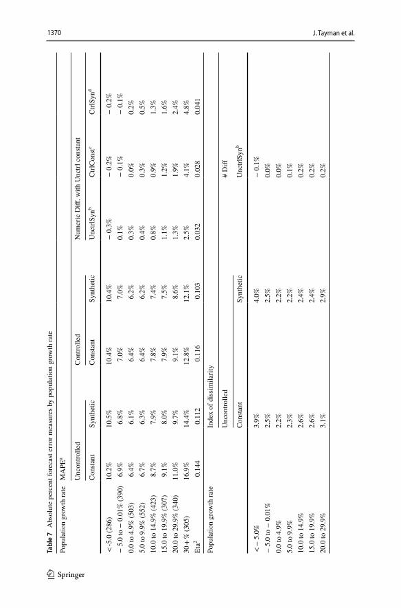
sign, than areas with stable growth patterns. UNCONST has lower accuracy com-pared to the other three alternatives in most growth rate categories. The main excep-tion is counties that experience a population loss. For the fastest declining coun-ties (< − 5.0%), the UNCONST MAPE is slightly lower at 10.2%; the MAPEs in this growth rate category are 10.4 or 10.5% for the other alternatives. For the more slowly declining counties (− 5.0 to − 0.01%), the UNCONST MAPE (6.9%) is 0.1 of a percentage point lower than the MAPEs for CRTLCONST and CTRLSYN, but 0.1 of a percentage point higher than the MAPE for UNCTRLSYN.

The ability of SYN and controlling to improve accuracy is directly related to the population growth rate. The numeric differences between UNCONST and the other alternatives widen consistently as the growth rate increases, with the largest differ-ences seen when both controlling and SYN are employed. The difference between UNCONST and CTRLSYN is − 0.2 percentage points in the fastest declining coun-ties and rises steadily reaching 4.8 percentage points in counties that grow by 30.0% or more. These results suggest that SYN and controlling will improve forecast accu-racy the greatest in counties with increasing growth rates.

A weaker direct relationship is seen between growth rate and IOD. The ETA2 falls into a narrow range of 0.087 and 0.089, which is lower than their counterparts (UNCONST and UNSYS) that range from 0.112 to 0.144. UNCONST has greater allocation error across age groups in all growth rate categories, except for the fastest declining counties where the IODs for UNCONST and UNSYN are 3.9% and 4.0%, respectively. However, there is very little difference in the IOD between UNCONST and UNSYN across growth rate categories with percentage point differences, ignor-ing the sign, ranging from 0.1 to 0.2%.

Finally, we examine the percent of counties where the APE for the age group average and IOD is smaller for SYN compared to CONST by population growth rate

Table 8 Percent of counties with lower synthetic APE and IOD by population growth rate

n in parenthesisExcludes counties where the synthetic and constant APEs and IOD are equala Average of the APEs across age groupsb Uncontrolled–controlled

Population growth rate APEa

Uncontrolled Controlled # Differenceb IODuncontrolled

< − 5.0% 53.4% 51.8% 1.6% 48.7%− 5.0 to − 0.01% 42.3% 48.6% − 6.3% 45.8%0.0 to 4.9% 58.7% 51.7% 7.0% 50.3%5.0 to 9.9% 61.4% 56.2% 5.3% 51.6%10.0 to 14.9% 69.3% 66.2% 3.1% 59.8%15.0 to 19.9% 70.4% 64.5% 5.9% 64.2%20.0 to 29.9% 71.0% 70.0% 1.0% 62.9%30+% 72.3% 71.1% 1.2% 56.7%Tau-C 0.136 0.125 0.011 0.059

1373

1 3


category. As Table 8 shows, the percentages are 50% or more for every population growth rate category, except for populations that declined more than − 5.0% in the uncontrolled IOD (48.7%). The other exceptions are for populations that declined less than − 5.0%, (uncontrolled APE (42.3%), controlled APE (48.6%), and uncon-trolled IOD (45.8%)). Excluding these exceptions, the percentages range from 51.7% in the controlled APE alternative in counties with a growth rate under 5.0% to 72.3% in the uncontrolled APE alternative for counties that grew 30% or more.

There is a direct relationship between the growth rate and the percentage of coun-ties where SYN outperforms CONST. This relationship is stronger in both APE alternatives (Tau-C of 0.136 and 0.125, respectively for the uncontrolled and con-trolled alternatives) compared to 0.059 for the uncontrolled IOD. These findings further support that SYN will be more useful for improving forecast accuracy in counties with increasing growth rates. Controlling, however, has an adverse impact as seen by comparing the APE alternatives. The uncontrolled percentages are larger (better SYN performance) than the controlled percentages in all growth rate catego-ries, except for counties that declined by less than − 5.0%, where the uncontrolled percentage was − 6.3 percentage points lower than the controlled percentage. For the other growth rate categories, the uncontrolled percentage exceeded the con-trolled percentage by between 1.0 percentage point (20.0 to − 29.9%) and 7.0 per-centage points (0.0 to − 4.9%).

Summary

The objectives of this first-ever evaluation of the H–P method in counties nationwide were to more rigorously test the efficacy of using a synthetic method to adjust CCRs and CWRs (SYN) over the horizon rather than holding them constant (CONST), which is the usual approach when applying this method. We also examined the per-formance of SYN and CONST when the total population forecast was determined from the age-gender forecast (a bottom-up model) and when the age-gender fore-casts were controlled to an independent county total population forecast. Out of a universe of 3,140 counties, we examined 3,106 counties that had constant bounda-ries between 1990 and 2010 and prepared a 10-year population forecast using a 2000 base year and a 2010 target year. We measured forecast accuracy, bias, and distribu-tional error across age groups using the MAPE, MALPE, IOD, and the percentage of counties where the absolute percent forecast error (APE) for SYN was smaller than that for CONST.

Our main findings are: (1) SYN lowers forecast error compared to CONST whether the forecasts are controlled or not; (2) controlling also leads to the improvements in forecast error, often exceeding those seen in SYN; and (3) using both SYN and controlling together has the greatest effect in reducing forecast error. These findings remain after controlling for population size and growth rate, but the positive impacts on forecast error of SYN and controlling are most evi-dent in counties with less than 30,000 population and that grow by 15% or more.


1 3

For the total population, UNSYN and CTRLPOP improve accuracy and reduce bias compared to UNCONST. The MAPEs for UNCONST, UNSYN, and CTLR-POP are 7.8%, 6.0%, and 6.0%, respectively. All three MAPEs show that the H–P method and the variants analyzed produce county-level total population forecasts that meet or exceed expected accuracy levels for 10-year county-level forecasts (Rayer et al. 2010; Smith et al. 2013, p. 365; Sprague 2013, p. 19). The MALPEs for UNCONST, UNSYN, and CTLRPOP are 4.3%, 2.5%, and 1.7%, respectively, which also indicate relatively low levels of bias in all alternatives.

In almost six out of ten counties, the UNSYN total population APE is smaller than the UNCONST APE and the accuracy gain in these counties (3.1 percentage points) is greater than the accuracy loss in the counties where the UNSYN APE is larger (− 2.3 percentage points). The advantages of UNSYN and CTRLPOP over UNCONST in reducing total population forecast errors are also widespread across the U.S. as demonstrated from the error patterns of counties within the 49 states analyzed in this paper.

The advantages of SYN over CONST in both the controlled and uncontrolled alternatives are also seen in the forecasts by age. The age-specific MAPEs for all four alternatives are in line with 10-year county forecasts produced using a modified Leslie Matrix model (Sprague 2013, p. 120) and are lower than 10-year forecasts produced for counties in Florida (Smith and Tayman 2003). The larger age-specific MAPEs in Florida’s counties are likely a result of the high migration and faster growth rates relative to counties nationwide.

UNSYN has greater accuracy than UNCONST in all age groups, except for ages < 10 (where the MAPEs are equal) and in ages 65–74 where the UNSYN MAPE is 0.4 of a percentage point larger). In general, UNSYN and CTLRSYN (both controlling and SYN) increase accuracy the greatest in ages 10–54 where most migration usually occurs. Compared to CTRLSYN, UNCONST increases the MAPE by between 2.1 and 2.8 percentage points in this age range. This suggests that adjusting and controlling CCRs better reflects future migration processes rather than holding them constant. CTRLSYN is less effective in terms of accuracy for the two oldest age groups (65–74 and 75+). For ages 65–74, the CTRLSYN and UNCONST alternatives have the same MAPEs. For ages 75+, the UNCONST MAPE (6.5%) is − 0.6 of a percentage point lower than the CTRLSYN MAPE (7.1%).

The patterns of forecast bias by age group are like those seen for forecast accu-racy but the improvements in bias compared to UNCONST are somewhat larger. Again, the greatest reduction in bias using SYN and controlling is in the peak migra-tion ages. Compared to CTRLSYN, UNCONST increases the MALPE by between 3.0 and 6.0 percentage points in ages 10–54. CTRLSYN is less effective in terms of bias for ages < 10 and 65–74. For ages < 10 the UNCONST MALPE (0.6%) is − 1.8 percentage points lower than the CTRLSYN MALPE (2.4%), and for ages 65–74 the UNCONST MAPE (− 0.3%) is − 0.9 of a percentage point lower than the CTRL-SYN MAPE (− 1.2%).

The allocation error across age groups is low in both UNSYN and UNCONST (IODs under 3%), and UNCONST’s IOD is only 0.1 percentage point less than UNSYN’s average allocation across age groups The advantages of SYN and control-ling over CONST in reducing population forecast error by age are also widespread

1375

1 3


across the U.S. as demonstrated from the MAPE of the average error across age groups of the counties within the 49 states analyzed in this paper.

We analyzed the average error across age groups by population size and growth rate. UNCONST has lower accuracy, as measured by the MAPE, in most size cat-egories compared to the other three alternatives. While the percentage point differ-ences between UNCONST and the other alternatives do not vary greatly by popula-tion size, SYN and controlling are more useful in improving forecast accuracy in counties with less than 30,000 persons.

In most growth rate categories, UNCONST has lower accuracy compared to the other three alternatives, as measured by the MAPE. The main exception is counties that experienced population losses, but the percentage point differences are small ranging between − 0.1% and − 0.3%. The standard H–P method applies a constant set of cohort growth rates to a beginning population, which can lead to a strong upward bias when applied to rapidly growing places. As such, it recommended that H–P forecasts of age and gender be controlled to an independent total popu-lation forecast (Baker et al. 2020; Smith et al. 2013, pp. 180–181; Swanson et al. 2010). Our analysis confirms the benefits of controlling as the numeric differences between UNCONST and the other alternatives widen consistently as the growth rate increases, indicating that SYN and controlling will improve forecast accuracy the greatest in counties with increasing growth rates.

Conclusion

The cohort-component method (CCM) is the most widely used approach for pro-ducing forecasts by age and sex and other demographic characteristics for counties and other higher-level geographies (Smith et al. 2013, p. 47). The CCM is very data intensive and requires at a minimum age-gender-specific death and migration rates and age-specific fertility rates. It also requires separate treatment of special popula-tions such as the military, college students, and jails and prisons (Baker et al. 2017, p. 47). However, the CCM can track changes in the components of change over the forecast horizon and allow simulations showing the impacts on the future population of alternative assumptions for these components.

The H–P method and its alternatives studied here are low cost and substantially less data intensive than the CCM and produce forecasts of the total population and demographic characteristics with similar levels of forecast error compared to its more data-intensive cousin (Hauer 2019; Smith and Tayman 2003; Sprague 2013; Wilson 2016). We know of at least one state demographic center that formally did its county forecasts using the CCM and switched to the H–P method controlled to independent total population forecast using similar extrapolation methods shown in this paper (Rayer and Wang 2020). While there are purposes for which the H–P method will not be useful, it is a viable alternative for county forecasts when only information on a future population and its composition is needed and not informa-tion on the components of population change and their effects. The H–P method does not provide information on the components of population change because it


1 3

uses CCRs that combine the effects of mortality and migration and CWRs that are very rough proxies to fertility rates.

While the standard H–P method (UNCONST) produces reasonable county-level forecasts of the total population and demographic characteristics, we have shown that H–P county-level forecasts are improved by adjusting the CCRs and CWRs using the synthetic method based on state trends over the horizon and by con-trolling the demographic characteristics to an independent total population in the county. Both modifications contribute to the decrease in forecast error compared to UNCONST that does not control to the total population of the county or modify the CCRs and CWRs. While H–P forecasts for counties can be improved by apply-ing controlling and SYN separately, the best (lower error) forecasts occur when both controlling and SYN are applied together. We recommend applying this dual approach when using the H–P method to prepare county population forecasts.

Another advantage of controlling and SYN is that they are low-cost modifications to the H–P method and are relatively simple to apply, making them easily accessible to those preparing population forecasts for counties. While some might question the accuracy of county total population controls produced from extrapolation methods, the preponderance of evidence suggests that these methods can produce total pop-ulation forecasts of comparable accuracy to those produced by more complication forecasting techniques (Green and Armstrong 2015; Hauer 2019; Rayer 2008; Smith et al. 2013, pp. 331–336). SYN requires state-level forecasts by age and gender and other characteristics if desired. Such forecasts are routinely prepared by most state population centers periodically after the latest census. Some agencies update their forecasts annually and others multiple times before the next census.

The H–P method has mainly been used for subcounty geographic areas where fertility, mortality, and migration are non-existent, unreliable, or difficult to obtain. A few studies have evaluated the impact of controlling and SYN at the census tract level. Baker et al. (2020) evaluated UNCONST and CTLRCONST and for cen-sus tracts nationwide, and Tayman and Swanson (2017) evaluated UNCONST and UNSYN for census tracts in the State of New Mexico. Given the synergies of con-trolling and SYN in reducing county forecast errors compared to UNCONST, it would be useful to study these synergies in broad-based samples of census tracts or even smaller geographic areas such as block groups and to investigate forecast hori-zons longer than 10 years.

Appendix

See Tables 9, 10, and 11.

1377

1 3


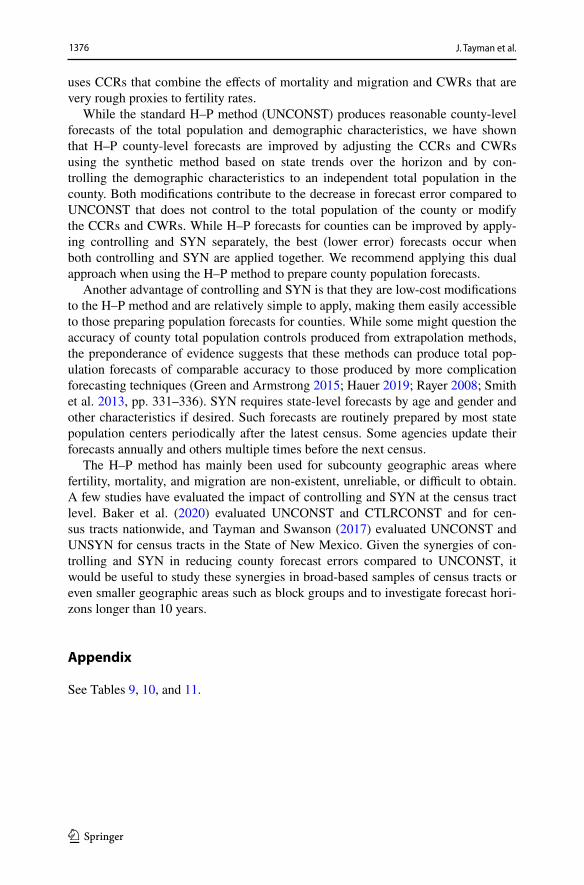
Table 9 Forecast MAPE by state, total population


Constant Synthetic Const & Syna Const. & Ctrlb

Alabama 7.2% 5.7% 6.1% 1.5% 1.1%Arizona 15.0% 9.9% 7.1% 5.1% 7.9%Arkansas 8.9% 5.3% 6.0% 3.6% 2.9%California 6.0% 6.0% 4.9% 0.0% 1.1%Colorado 25.3% 20.1% 12.1% 5.2% 13.2%Connecticut 4.3% 2.2% 2.6% 2.1% 1.7%Delaware 7.9% 7.4% 5.5% 0.5% 2.4%Florida 8.3% 6.6% 6.5% 1.7% 1.8%Georgia 10.2% 8.4% 7.3% 1.8% 2.9%Hawaii 41.1% 41.0% 17.7% 0.1% 23.4%Idaho 12.2% 10.5% 8.4% 1.7% 3.8%Illinois 4.8% 4.9% 4.6% − 0.1% 0.2%Indiana 5.0% 4.3% 4.3% 0.7% 0.7%Iowa 3.5% 3.4% 4.2% 0.1% − 0.7%Kansas 6.4% 5.7% 5.9% 0.7% 0.5%Kentucky 6.7% 5.7% 4.7% 1.0% 2.0%Louisiana 8.8% 8.8% 8.8% 0.0% 0.0%Maine 5.3% 5.2% 4.2% 0.1% 1.1%Maryland 4.4% 4.6% 3.8% − 0.2% 0.6%Massachusetts 7.2% 7.3% 4.1% − 0.1% 3.1%Michigan 10.8% 9.3% 6.0% 1.5% 4.8%Minnesota 5.2% 5.0% 4.4% 0.2% 0.8%Mississippi 10.2% 7.8% 8.4% 2.4% 1.8%Missouri 6.7% 5.7% 4.2% 1.0% 2.5%Montana 7.0% 6.9% 6.1% 0.1% 0.9%Nebraska 5.8% 5.2% 5.8% 0.6% 0.0%Nevada 20.4% 15.1% 11.2% 5.3% 9.2%New Hampshire 3.7% 3.8% 3.1% − 0.1% 0.6%New Jersey 3.5% 3.7% 2.6% − 0.2% 0.9%New Mexico 16.6% 14.3% 11.8% 2.3% 4.8%New York 3.7% 4.5% 2.8% − 0.8% 0.9%North Carolina 5.5% 4.8% 5.0% 0.7% 0.5%North Dakota 7.7% 7.2% 7.4% 0.5% 0.3%Ohio 3.0% 2.9% 3.0% 0.1% 0.0%Oklahoma 5.9% 6.1% 5.2% − 0.2% 0.7%Oregon 8.9% 6.5% 5.1% 2.4% 3.8%Pennsylvania 4.6% 4.5% 4.2% 0.1% 0.4%Rhode Island 2.9% 3.1% 2.1% − 0.2% 0.8%South Carolina 7.4% 7.0% 6.8% 0.4% 0.6%South Dakota 5.9% 5.4% 5.9% 0.5% 0.0%Tennessee 8.4% 5.3% 5.0% 3.1% 3.4%


1 3

a Uncontrolled constant–uncontrolled syntheticb Uncontrolled constant–controlled

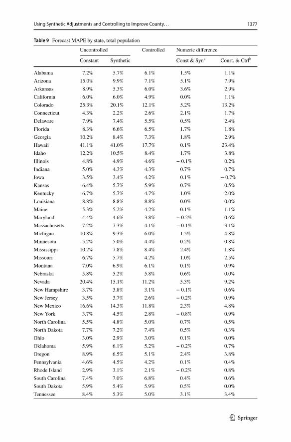
Table 9 (continued)


Constant Synthetic Const & Syna Const. & Ctrlb

Texas 10.4% 9.7% 8.1% 0.7% 2.3%Utah 10.9% 8.8% 6.3% 2.1% 4.6%Vermont 4.0% 4.2% 3.0% − 0.2% 1.0%Virginia 7.3% 7.8% 6.5% − 0.5% 0.8%Washington 7.7% 5.2% 4.5% 2.5% 3.2%West Virginia 5.9% 5.8% 6.4% 0.1% − 0.5%Wisconsin 6.7% 6.0% 5.3% 0.7% 1.4%Wyoming 10.8% 8.7% 7.9% 2.1% 2.9%

1379

1 3


Table 10 Forecast MALPE by state, total population

Uncontrolled Controlled Numeric differencea

Constant Synthetic Const & Synb Syn & Ctrlc

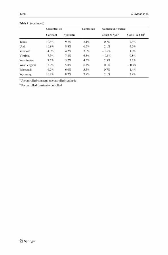
Alabama 5.4% 1.6% 3.3% 3.8% 2.1%Arizona 11.3% 3.6% 0.8% 7.7% 10.5%Arkansas 8.6% 3.2% 4.6% 5.4% 4.0%California 3.4% 3.1% 0.2% 0.3% 3.2%Colorado 23.4% 17.3% 9.1% 6.1% 14.3%Connecticut − 4.3% − 1.1% − 2.0% 3.3% 2.3%Delaware − 0.5% − 2.1% − 4.5% − 1.6% − 4.0%Florida 5.5% − 0.7% − 2.0% 4.8% 3.5%Georgia 6.6% 0.5% 0.1% 6.1% 6.5%Hawaii 35.9% 39.1% 13.6% − 3.2% 22.3%Idaho 8.4% 0.6% 2.0% 7.8% 6.4%Illinois 1.3% − 2.0% 0.4% − 0.7% 0.9%Indiana 3.3% 0.7% 2.0% 2.6% 1.3%Iowa 1.5% 0.9% 2.6% 0.6% − 1.1%Kansas 3.4% 0.8% 3.9% 2.6% − 0.5%Kentucky 5.1% 2.7% 2.6% 2.4% 2.5%Louisiana 4.0% 2.6% 2.9% 1.4% 1.1%Maine − 3.0% 0.7% − 0.9% 2.3% 2.1%Maryland 0.0% 1.7% − 1.1% − 1.7% − 1.1%Massachusetts 5.7% 6.0% 2.9% − 0.3% 2.8%Michigan 10.0% 7.8% 5.0% 2.2% 5.0%Minnesota 2.3% 1.4% 1.0% 0.9% 1.3%Mississippi 9.0% 4.5% 5.3% 4.5% 3.7%Missouri 4.7% 2.5% 1.6% 2.2% 3.1%Montana 1.3% − 0.4% 1.2% 0.9% 0.1%Nebraska 2.3% − 0.9% 3.5% 1.4% − 1.2%Nevada 10.1% − 7.9% − 1.5% 2.2% 8.6%New Hampshire − 0.1% − 0.5% − 0.9% − 0.4% − 0.8%New Jersey 1.5% 1.8% 0.6% − 0.3% 0.9%New Mexico 13.4% 7.3% 7.5% 6.1% 5.9%New York − 1.1% − 2.9% − 0.4% − 1.8% 0.7%North Carolina 2.9% 0.2% − 0.3% 2.7% 2.6%North Dakota − 5.8% − 3.2% 0.7% 2.6% 5.1%Ohio 1.5% 0.6% 0.9% 0.9% 0.6%Oklahoma 0.4% − 3.0% − 0.6% − 2.6% − 0.2%Oregon 7.8% 1.0% 2.8% 6.9% 5.0%Pennsylvania − 0.4% 0.5% 0.7% − 0.1% − 0.3%Rhode Island 2.5% 2.9% 2.1% − 0.4% 0.4%South Carolina 3.7% 2.2% 2.2% 1.5% 1.5%South Dakota 2.0% 0.4% 3.0% 1.6% − 1.0%Tennessee 7.8% 2.7% 2.8% 5.1% 5.0%


1 3

a Based on the absolute value of MALPEb Uncontrolled constant–uncontrolled syntheticc Uncontrolled constant–controlled

Table 10 (continued)

Uncontrolled Controlled Numeric differencea

Constant Synthetic Const & Synb Syn & Ctrlc

Texas 4.8% 2.5% 0.8% 2.3% 4.0%Utah 7.8% 0.4% − 1.3% 7.4% 6.5%Vermont 3.7% 3.9% 2.7% − 0.2% 1.0%Virginia 1.7% 3.4% 0.1% − 1.7% 1.6%Washington 6.3% − 0.7% 0.9% 5.6% 5.4%West Virginia − 1.4% 0.8% − 0.5% 0.6% 0.9%Wisconsin 5.1% 3.4% 3.2% 1.7% 1.9%Wyoming − 5.8% − 0.3% − 3.7% 5.5% 2.1%

1381

1 3


Table 11 Forecast MAPE by state, average APE across age groups



Alabama 7.6% 6.6% 6.9% 7.0% 1.0% 0.7% 0.6%Arizona 15.3% 11.3% 9.2% 9.3% 4.0% 6.1% 6.0%Arkansas 9.1% 6.7% 7.4% 7.2% 2.4% 1.7% 1.9%California 7.2% 7.6% 7.1% 7.1% − 0.4% 0.1% 0.1%Colorado 23.8% 19.7% 15.5% 14.0% 4.1% 8.3% 9.8%Connecticut 5.1% 3.7% 4.0% 4.0% 1.4% 1.1% 1.1%Delaware 8.6% 8.2% 7.7% 7.9% 0.4% 0.9% 0.7%Florida 9.3% 9.6% 8.4% 9.5% − 0.3% 0.9% − 0.2%Georgia 11.1% 9.9% 9.9% 9.4% 1.2% 1.2% 1.7%Hawaii 39.8% 40.7% 20.6% 21.0% − 0.9% 19.2% 18.8%Idaho 13.1% 11.4% 11.1% 10.5% 1.7% 2.0% 2.6%Illinois 6.2% 6.3% 6.3% 6.2% − 0.1% − 0.1% 0.0%Indiana 6.4% 6.0% 6.1% 5.8% 0.4% 0.3% 0.6%Iowa 5.6% 5.3% 6.1% 5.8% 0.3% − 0.5% − 0.2%Kansas 8.5% 7.8% 8.5% 8.1% 0.7% 0.0% 0.4%Kentucky 7.9% 7.2% 7.0% 6.7% 0.7% 0.9% 1.2%Louisiana 9.8% 9.9% 10.0% 10.0% − 0.1% − 0.2% − 0.2%Maine 5.9% 6.1% 4.8% 5.5% − 0.2% 1.1% 0.4%Maryland 5.7% 6.2% 5.2% 5.7% − 0.5% 0.5% 0.0%Massachusetts 7.5% 7.2% 5.4% 5.0% 0.3% 2.1% 2.5%Michigan 11.2% 9.6% 8.1% 7.2% 1.6% 3.1% 4.0%Minnesota 7.0% 6.7% 6.7% 6.2% 0.3% 0.3% 0.8%Mississippi 10.4% 8.4% 9.2% 8.9% 2.0% 1.2% 1.5%Missouri 7.8% 6.9% 6.7% 6.2% 0.9% 1.1% 1.6%Montana 10.5% 10.1% 9.9% 9.5% 0.4% 0.6% 1.0%Nebraska 9.0% 8.0% 9.1% 8.6% 1.0% − 0.1% 0.4%Nevada 19.5% 16.7% 13.7% 13.6% 2.8% 5.8% 5.9%New Hampshire 5.0% 4.7% 4.4% 4.1% 0.3% 0.6% 0.9%New Jersey 5.3% 5.3% 4.9% 4.7% 0.0% 0.4% 0.6%New Mexico 16.4% 14.4% 12.4% 12.8% 2.0% 4.0% 3.6%New York 5.3% 6.0% 4.7% 5.5% − 0.7% 0.6% − 0.2%North Carolina 7.5% 6.7% 7.6% 7.0% 0.8% − 0.1% 0.5%North Dakota 9.9% 9.6% 10.9% 10.6% 0.3% − 1.0% − 0.7%Ohio 5.1% 4.8% 5.3% 4.9% 0.3% − 0.2% 0.2%Oklahoma 7.5% 7.5% 7.3% 7.1% 0.0% 0.2% 0.4%Oregon 10.1% 8.5% 8.2% 7.4% 1.6% 1.9% 2.7%Pennsylvania 5.5% 5.7% 5.1% 5.4% − 0.2% 0.4% 0.1%Rhode Island 4.6% 3.8% 4.3% 2.8% 0.8% 0.3% 1.8%South Carolina 8.1% 7.5% 7.9% 7.5% 0.6% 0.2% 0.6%South Dakota 9.0% 8.4% 9.3% 8.9% 0.6% − 0.3% 0.1%Tennessee 8.6% 6.2% 6.9% 6.1% 2.4% 1.7% 2.5%


1 3

Open Access This article is licensed under a Creative Commons Attribution 4.0 International License, which permits use, sharing, adaptation, distribution and reproduction in any medium or format, as long as you give appropriate credit to the original author(s) and the source, provide a link to the Creative Com-mons licence, and indicate if changes were made. The images or other third party material in this article are included in the article’s Creative Commons licence, unless indicated otherwise in a credit line to the material. If material is not included in the article’s Creative Commons licence and your intended use is not permitted by statutory regulation or exceeds the permitted use, you will need to obtain permission directly from the copyright holder. To view a copy of this licence, visit http:// creat iveco mmons. org/ licen ses/ by/4. 0/.

References

Baker, J., Alcantara, A., Ruan, X., Watkins, K., & Vasan, S. (2014). Spatial weighing improves accu-racy in small area demographic forecasts of urban census tract population. Journal of Population Research, 31, 345–359.

Baker, J., Swanson, D. A., & Tayman, J. (2020). The accuracy of Hamilton-Perry population projections for census tracts in the United States. Population Research and Policy Review. https:// doi. org/ 10. 1007/ s11113- 020- 09601-y.

Baker, J., Swanson, D. A., Tayman, J., & Tedrow, L. M. (2017). Cohort change ratios and their applica-tions. Dordrecht: Springer.

Duncan, O. D., Cuzzort, R. P., & Duncan, B. (1961). Statistical geography: Problems in analyzing area data. Glencoe, IL: Free Press.

Fonseca, L., & Tayman, J. (1989). Postcensal estimates of household income distributions. Demography, 26, 149–159.

Green, K. C., & Armstrong, J. S. (2015). Simple versus complex forecasting: The evidence. Journal of Business Research, 68, 1678–1685.

Hamilton, C. H., & Perry, J. (1962). A short method for projecting population by age from one decennial census to another. Social Forces, 41, 163–170.

Hardy, G., & Wyatt, F. (1911). Report of the actuaries in relation to the scheme of insurance against sick-ness, disablement, etc. Journal of the Institute of Actuaries, XLV, 406–433.

Hauer, M. E. (2019). Population projections for U.S. counties by age, sex, and race controlled to shared socioeconomic pathway. Sci Data. https:// doi. org/ 10. 1038/ sdata. 219.5.

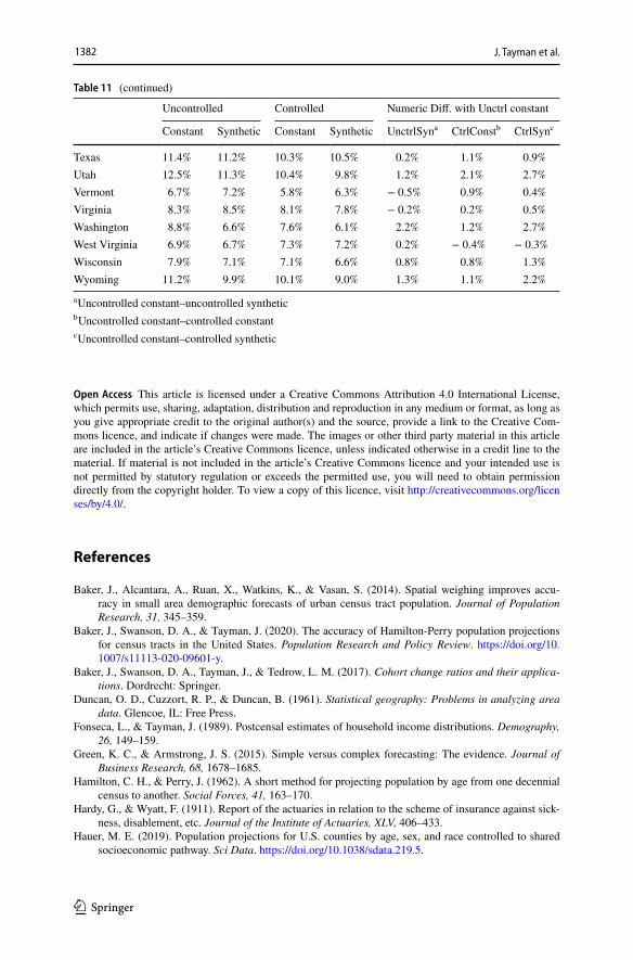
a Uncontrolled constant–uncontrolled syntheticb Uncontrolled constant–controlled constantc Uncontrolled constant–controlled synthetic

Table 11 (continued)



Texas 11.4% 11.2% 10.3% 10.5% 0.2% 1.1% 0.9%Utah 12.5% 11.3% 10.4% 9.8% 1.2% 2.1% 2.7%Vermont 6.7% 7.2% 5.8% 6.3% − 0.5% 0.9% 0.4%Virginia 8.3% 8.5% 8.1% 7.8% − 0.2% 0.2% 0.5%Washington 8.8% 6.6% 7.6% 6.1% 2.2% 1.2% 2.7%West Virginia 6.9% 6.7% 7.3% 7.2% 0.2% − 0.4% − 0.3%Wisconsin 7.9% 7.1% 7.1% 6.6% 0.8% 0.8% 1.3%Wyoming 11.2% 9.9% 10.1% 9.0% 1.3% 1.1% 2.2%

http://creativecommons.org/licenses/by/4.0/

http://creativecommons.org/licenses/by/4.0/

https://doi.org/10.1007/s11113-020-09601-y

https://doi.org/10.1007/s11113-020-09601-y

https://doi.org/10.1038/sdata.219.5

1383

1 3


Kodiko, H. (2014). Subnational projections methods: Application to the counties in the former Nyanza Province, Kenya. (Master’s Thesis), University of Nairobi, Nairobi, Kenya.

Massey, D. S., & Denton, N. A. (1988). The dimensions of residential segregation. Social Forces, 67, 163–184.

Pittenger, D. (1976). Projecting state and local populations. Cambridge, MA: Ballinger.Rayer, S. (2007). Population forecast accuracy: Does the choice of summary measure of error matter?

Population Research and Policy Review, 26, 163–184.Rayer, S. (2008). Population forecast errors: A primer for planners. Journal of Planning Education and

Research, 27, 417–430.Rayer, S., Smith, S. K., & Tayman, J. (2010). Empirical prediction intervals for county-level forecasts.

Population Research and Policy Review, 28, 773–793.Rayer, S., & Wang, Y. (2020). Methodology for constructing population projections by age, sex, race,

and Hispanic Origin for Florida and its counties, 2020–2045, with estimates for 2019. Gainesville, FL: University of Florida.

Smith, S. K., & Shahidullah, M. (1995). An evaluation of population projections errors by census tract. Journal of the American Statistical Association, 90, 64–71.

Smith, S. K., & Tayman, J. (2003). An evaluation of population projections by age. Demography, 40, 741–757.

Smith, S. K., Tayman, J., & Swanson, D. A. (2013). A practitioner’s guide to state and local population projection. Dordrecht: Springer.

Sprague, W. W. (2013). Wood’s method: A method for fitting Leslie matrices from age-sex population data, with some practical applications. (Dissertation), University of California, Berkeley, Berkeley, CA.

Swanson, D. A. (2015). On the relationship among values of the same summary measure of error when it is used across multiple characteristics at the same point in time: An examination of MALPE and MAPE. Review of Economics and Finance, 5, 1–14.

Swanson, D. A., Schlottmann, A., & Schmidt, R. (2010). Forecasting the population of census tracts by age and sex: An example of the Hamilton-Perry method in action. Population Research and Policy Review, 29, 47–63.

Swanson, D. A., & Tayman, J. (2012). Subnational population estimates. Dordrecht: Springer.Swanson, D. A., & Tayman, J. (2017). A long-term test of the accuracy of the Hamilton-Perry method for

forecasting state populations by age. In D. A. Swanson (Ed.), The Frontiers of Applied Demography (pp. 491–514). Dordrecht: Springer.

Swanson, D. A., Tayman, J., & Bryan, T. (2011). MAPE-R: A rescaled measure of accuracy for cross-sectional, sub-national forecasts. Journal of Population Research, 28, 225–243.

Swanson, D. A., Tayman, J., McKibben, J., & Cropper, M. (2012). A “blind” ex post facto evaluation of total population and total household forecast for small areas made by five vendors for 2010: Results by geography and error criteria. Waterloo, Ontario: Paper presented at the Canadian Population Society.

Tayman, J., Smith, S. K., & Rayer, S. (2011). Evaluating population forecast accuracy: A regression approach using county data. Population Research and Policy Review, 30, 235–262.

Tayman, J., & Swanson, D. A. (2017). Using modified cohort change and child-woman ratios in the Ham-ilton Perry forecasting method. Journal of Population Research, 34(3), 209–231.

Williamson, P. (2013). An evaluation of two synthetic small area microsimulation methodologies: Syn-thetic reconstruction and combinatorial optimisation. In R. Tanton & K. L. Edwards (Eds.), Spatial microsimulation: A reference guide for users (pp. 227–258). Heidelberg: Springer.

Wilson, T. (2016). Evaluation of alternative Cohort-Component models for local area population fore-casts. Population Research and Policy Review, 35, 241–261.

Publisher’s Note Springer Nature remains neutral with regard to jurisdictional claims in published maps and institutional affiliations.

Using Synthetic Adjustments and Controlling to Improve ...

Documents

Transcript of Using Synthetic Adjustments and Controlling to Improve ...