USING SPATIOTEMPORAL RELATIONAL RANDOM FORESTS TO … · USING SPATIOTEMPORAL RELATIONAL RANDOM...
28
USING SPATIOTEMPORAL RELATIONAL RANDOM FORESTS TO IMPROVE OUR UNDERSTANDING OF SEVERE WEATHER PROCESSES AMY MCGOVERN 1 , DAVID JOHN GAGNE II 2 , NATHANIEL TROUTMAN 1 , RODGER A. BROWN 3 , JEFFREY BASARA 4 , AND JOHN K. WILLIAMS 5 Abstract. Major severe weather events can cause a significant loss of life and property. We seek to revolutionize our understanding of and our ability to predict such events through the mining of severe weather data. Because weather is inherently a spatiotemporal phenomenon, mining such data requires a model capable of representing and reasoning about complex spatiotemporal dynamics, including temporally and spatially varying attributes and relationships. We introduce an augmented version of the Spatiotemporal Relational Random Forest, which is a Random Forest that learns with spatiotemporally varying relational data. Our algorithm maintains the strength and performance of Random Forests but extends their applicability, including the estimation of variable importance, to complex spatiotemporal relational domains. We apply the augmented Spatiotemporal Relational Random Forest to three severe weather data sets. These are: predicting atmospheric turbulence across the continental United States, examining the formation of tornadoes near strong frontal boundaries, and understanding the spatial evolution of drought across the southern plains of the United States. The results on such a wide variety of real-world domains demonstrate the extensive applicability of the Spatiotemporal Relational Random Forest. Our long-term goal is to significantly improve the ability to predict and warn about severe weather events. We expect that the tools and techniques we develop will be applicable to a wide range of complex spatiotemporal phenomena. Keywords: spatiotemporal data mining, statistical relational learning, severe weather, random forests 1. Introduction The majority of real-world data, such as the weather data studied here, varies as a function of both space and time. For example, a thunderstorm evolves over time and may eventually produce a tornado through the spatiotemporal interaction of components of the storm. In this paper, we introduce and validate a greatly augmented version of the Spatiotemporal Relational Random Forest (SRRF) algorithm for use with severe weather data. The SRRF is a Random Forest (RF) [6] approach that directly reasons with spatiotemporal relational data and is a major contribution to the research in spatiotemporal relational models. Due to the increased complexity introduced by spatiotemporally varying data, most data mining algorithms ignore one or both of these aspects (e.g. temporal only relational models such as [13, 20, 34]) and our recent work is the only work that we know of that addresses both spatiotemporal and relational data [23, 38, 3]. Our work is motivated by and validated in three real-world earth science domains. The first is predicting thunderstorm-induced turbulence as experienced by aircraft, focusing on the continental United States. Such turbulence is inherently spatiotemporal, with thunderstorms causing increased turbulence on a short time scale in the local region around a storm and also on a longer time scale across a greater spatial extent. With this domain, our goal is to enhance the current operational products that provide turbulence prediction to aviation interests by improving the spatiotemporal 1 School of Computer Science, University of Oklahoma, [email protected], [email protected] 2 School of Meteorology, University of Oklahoma, [email protected] 3 NOAA/National Severe Storms Laboratory, [email protected] 4 Oklahoma Climatological Survey, [email protected] 5 Research Applications Laboratory, National Center for Atmospheric Research, [email protected]. 1
Transcript of USING SPATIOTEMPORAL RELATIONAL RANDOM FORESTS TO … · USING SPATIOTEMPORAL RELATIONAL RANDOM...
USING SPATIOTEMPORAL RELATIONAL RANDOM FORESTS TO IMPROVE
OUR UNDERSTANDING OF SEVERE WEATHER PROCESSES
AMY MCGOVERN1, DAVID JOHN GAGNE II2, NATHANIEL TROUTMAN1, RODGER A. BROWN3,JEFFREY BASARA4, AND JOHN K. WILLIAMS5
Abstract. Major severe weather events can cause a significant loss of life and property. We seekto revolutionize our understanding of and our ability to predict such events through the mining
of severe weather data. Because weather is inherently a spatiotemporal phenomenon, mining
such data requires a model capable of representing and reasoning about complex spatiotemporaldynamics, including temporally and spatially varying attributes and relationships. We introduce
an augmented version of the Spatiotemporal Relational Random Forest, which is a Random Forest
that learns with spatiotemporally varying relational data. Our algorithm maintains the strengthand performance of Random Forests but extends their applicability, including the estimation of
variable importance, to complex spatiotemporal relational domains. We apply the augmented
Spatiotemporal Relational Random Forest to three severe weather data sets. These are: predictingatmospheric turbulence across the continental United States, examining the formation of tornadoes
near strong frontal boundaries, and understanding the spatial evolution of drought across thesouthern plains of the United States. The results on such a wide variety of real-world domains
demonstrate the extensive applicability of the Spatiotemporal Relational Random Forest. Our
long-term goal is to significantly improve the ability to predict and warn about severe weatherevents. We expect that the tools and techniques we develop will be applicable to a wide range of
complex spatiotemporal phenomena.
Keywords: spatiotemporal data mining, statistical relational learning, severe weather, randomforests
1. Introduction
The majority of real-world data, such as the weather data studied here, varies as a function ofboth space and time. For example, a thunderstorm evolves over time and may eventually producea tornado through the spatiotemporal interaction of components of the storm. In this paper, weintroduce and validate a greatly augmented version of the Spatiotemporal Relational Random Forest(SRRF) algorithm for use with severe weather data. The SRRF is a Random Forest (RF) [6]approach that directly reasons with spatiotemporal relational data and is a major contribution tothe research in spatiotemporal relational models. Due to the increased complexity introduced byspatiotemporally varying data, most data mining algorithms ignore one or both of these aspects(e.g. temporal only relational models such as [13, 20, 34]) and our recent work is the only work thatwe know of that addresses both spatiotemporal and relational data [23, 38, 3].
Our work is motivated by and validated in three real-world earth science domains. The first ispredicting thunderstorm-induced turbulence as experienced by aircraft, focusing on the continentalUnited States. Such turbulence is inherently spatiotemporal, with thunderstorms causing increasedturbulence on a short time scale in the local region around a storm and also on a longer time scaleacross a greater spatial extent. With this domain, our goal is to enhance the current operationalproducts that provide turbulence prediction to aviation interests by improving the spatiotemporal
1School of Computer Science, University of Oklahoma, [email protected], [email protected] of Meteorology, University of Oklahoma, [email protected]/National Severe Storms Laboratory, [email protected] Climatological Survey, [email protected] Applications Laboratory, National Center for Atmospheric Research, [email protected].
1

reasoning of the models. Prior work demonstrated that RFs were a promising approach in theturbulence domain [44]. We are currently performing case studies of the SRRF and investigatingthe possibility of integrating the trained SRRFs into an operational turbulence guidance product.
Spatiotemporal data mining using the SRRFs can aid the development of effective turbulencepredictions by uncovering and exploiting relationships between storm features and environmentalcharacteristics that confirm and go beyond mechanisms that are currently understood by atmosphericscientists. In doing so, it has the potential to not only create practical predictive systems, but alsoto improve scientific understanding of turbulence.
The second domain is that of understanding and predicting tornadoes. The results presented inthis paper are a piece of a larger overall project focusing on revolutionizing our understanding oftornadoes. In this paper, we look at the interaction of tornadic and nontornadic supercell thunder-storms with their environment as they moved across the state of Oklahoma over a 10 year period.Prior tornado research has found that 70% of strong tornadoes in 1995 were located within 30 km ofa front [22]. The goal of this part of the project is to use SRRFs to perform a climatological studyof tornadic supercell thunderstorms and how the variations in the surface environment affect them.
The National Oceanic and Atmospheric Administration’s National Weather Service has a goal ofdeveloping Warn-on-Forecast capabilities by 2020, instead of the current warn on detection approach[36]. The Warn-on-Forecast concept hopes to increase the lead time of severe weather and tornadowarnings by accurately predicting the time and location of severe storms using numerical models.Our data mining approach promises to identify those within-storm features that discriminate betweenstorms that will produce tornadoes and those that will not. It can be directly used within thenumerical modeling of storms and given to the weather forecasters who issue the warnings.
In the third domain, we study the progression of droughts across the Southern Great Plains fora 134 year period. Drought is a spatiotemporal phenomenon that operates on a very different timescale than tornadoes or turbulence. While those appear and disappear relatively quickly, droughttakes months to years to progress. The goal with this work is to improve the prediction of droughtthrough an improved understanding of how drought moves in each local region.
RFs [6] are a simple and powerful algorithm with a strong track record (e.g., [33, 26, 14, 4, 43]).RFs learn an ensemble of C4.5 [31] trees, each of which is trained on a separate bootstrap resampleddataset and using a different subset of the attributes. The power of the approach comes from thedifferences in the trees, which enable the forest to capture more expressive concepts than with asingle decision tree. Since the trees are each trained on a different subset of the data, they can focuson different aspects of the overall classification problem. In addition to their predictive capabilities,one of the reasons that RFs are so popular is their ability to analyze the variables for their overallimportance at predicting the concept.
We introduced a preliminary version of the SRRFs in [38] and preliminary results in these domainsin [24]. This paper represents a significant extension as outlined below.
(1) The SRRF algorithm has been extended to address variable importance of spatiotemporalrelational data. Since we are working directly with the domain scientists, the human inter-pretability of the models is critical. A single tree can be examined easily but an entire forestis more difficult to analyze, making the variable importance aspect crucial. This is a majorextension from [38] and was reported in [24].
(2) We have further enhanced our ability to analyze the trees by enabling the domain scientiststo examine the valid ranges of specific attribute values in each tree in the forest. For example,instead of a distinction that asks “Is there an updraft with maximum speed at least 15.3m s−1?”, we provide the range of the attribute where performance is the same. This is anextension of our work from [24].
(3) Our underlying Spatiotemporal Relational Probability Tree (SRPT, [23]) algorithm has beenconsiderably enhanced to improve the spatiotemporal distinctions. This gives us the abilityto represent temporally and spatially varying fields within objects, which significantly aug-ments our ability to mine and understand severe weather. The spatiotemporal fields were
2
in progress for the [24] paper and all of the results reported here use these fields. This is asignificant extension of the work reported in [24].
(4) We thoroughly explore the parameter space of the algorithm on all of our domains. Dueto space limitations, these results were not reported in [24] but they are included in theirentirety here. We have also expanded the data sets used in the parameter space experiments.
(5) We have significantly extended the application to multiple real-world severe weather do-mains, which is a significant extension of the work reported in [38]. Although the domainsremain the same as those presented in [24], all of the results and analyses are new to thispaper.
2. Growing SRRFs
Growing a SRRF is very similar to the approach used to grow an RF [6] with a few critical changesrequired by the nature of the spatiotemporal relational data. Algorithms 1, 2, and 3 describe thelearning process in detail. Before discussing these, we describe how we represent the spatiotemporalrelational data for efficient model learning.
The data are represented as spatiotemporal attributed relational graphs, as we first presented in[23]. This representation is an extension of the attributed graph approach [29, 28, 19] to handlespatiotemporally varying data. All objects, such as aircraft, tornadoes, or hail cores, are representedby vertices in the graph. Relationships between the objects are represented using edges. With thesevere weather data, the majority of the relationships are spatial. Both objects and relationships canhave attributes associated with them and these attributes can vary both spatially and temporally.In the case of a spatially or spatiotemporally varying attribute, the data are represented as either ascalar or a vector field, depending on the nature of the data. The ability to represent spatial fieldsof objects is a key addition to the SRRF results presented here. This field can be two or threedimensional for space and can also vary as a function of time. In addition to attributes varying overspace and time, the existence of objects and relationships can also vary as a function of time. If anobject or a relationship is dynamic, it has a starting and an ending time associated with it.
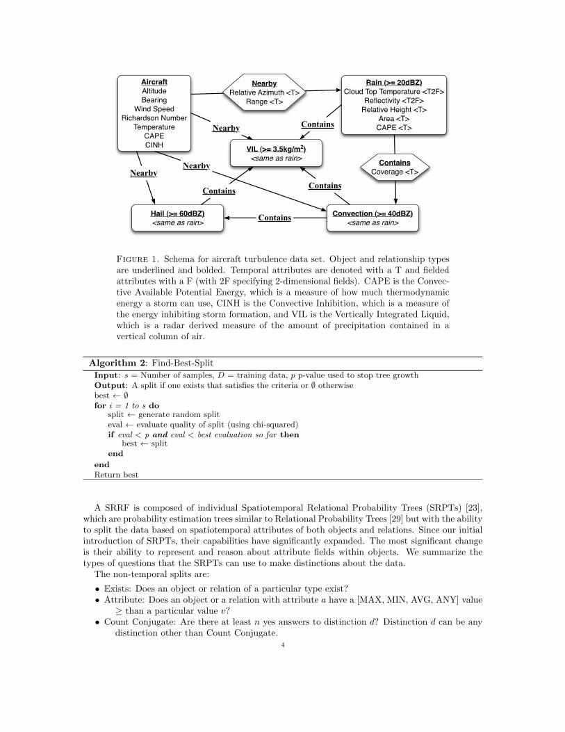
To illustrate the data representation, Figure 1 shows the schema for the turbulence data. Allobjects and relations are required to be assigned a type. In this case, the attributes on the rain, hail,convection, and vertically integrated liquid objects are all temporal or 2-dimensional spatiotemporalscalar fields. The attributes on the aircraft object are all static as they are measured at a singlemoment in time. Note that the schema shows the types of objects and relationships possible butany specific graph can vary in the number of such objects present. For example, all graphs in theturbulence data will have an aircraft object but they may have any number (including 0) of rain,hail, and convective regions as defined by the weather nearby the aircraft.
Algorithm 1: Grow-SRPT
Input: s = Number of distinctions to sample, D = training data, m = Maximum depth of tree, d =current tree depth, p p-value used to stop tree growth
Output: An SRPTif d ≤ m then
tree ← Find-Best-Split(D,s,p)if tree 6= ∅ then
for all possible values v in split dotree.addChild(Grow-SRPT(D where split = v))
endReturn tree
end
endReturn leaf node
3
AircraftAltitudeBearing
Wind SpeedRichardson Number
TemperatureCAPECINH
Hail (>= 60dBZ)<same as rain>
Convection (>= 40dBZ)<same as rain>
Rain (>= 20dBZ)Cloud Top Temperature <T2F>
Reflectivity <T2F>Relative Height <T>
Area <T>CAPE <T>
VIL (>= 3.5kg/m2)<same as rain> Contains
Coverage <T>
Contains
Contains
Contains
Contains
NearbyRelative Azimuth <T>
Range <T>
Nearby
Nearby
Nearby
Figure 1. Schema for aircraft turbulence data set. Object and relationship typesare underlined and bolded. Temporal attributes are denoted with a T and fieldedattributes with a F (with 2F specifying 2-dimensional fields). CAPE is the Convec-tive Available Potential Energy, which is a measure of how much thermodynamicenergy a storm can use, CINH is the Convective Inhibition, which is a measure ofthe energy inhibiting storm formation, and VIL is the Vertically Integrated Liquid,which is a radar derived measure of the amount of precipitation contained in avertical column of air.
Algorithm 2: Find-Best-Split
Input: s = Number of samples, D = training data, p p-value used to stop tree growthOutput: A split if one exists that satisfies the criteria or ∅ otherwisebest ← ∅for i = 1 to s do
split ← generate random spliteval ← evaluate quality of split (using chi-squared)if eval < p and eval < best evaluation so far then
best ← splitend
endReturn best
A SRRF is composed of individual Spatiotemporal Relational Probability Trees (SRPTs) [23],which are probability estimation trees similar to Relational Probability Trees [29] but with the abilityto split the data based on spatiotemporal attributes of both objects and relations. Since our initialintroduction of SRPTs, their capabilities have significantly expanded. The most significant changeis their ability to represent and reason about attribute fields within objects. We summarize thetypes of questions that the SRPTs can use to make distinctions about the data.
The non-temporal splits are:
• Exists: Does an object or relation of a particular type exist?• Attribute: Does an object or a relation with attribute a have a [MAX, MIN, AVG, ANY] value
≥ than a particular value v?• Count Conjugate: Are there at least n yes answers to distinction d? Distinction d can be any
distinction other than Count Conjugate.4
• Structural Conjugate: Is the answer to distinction d related to an object of type t through arelation of type r? Distinction d can be any distinction other than Structural Conjugate.
The temporal splits are:
• Temporal Exists: Does an object or a relation of a particular type exist for time period t?• Temporal Ordering: Do the matching items from basic distinction a occur in a temporal
relationship with the matching items from basic distinction b? The seven types of temporalordering are: before, meets, overlaps, equals, starts, finishes, and during [2].
• Temporal Partial Derivative: Is the partial derivative with respect to time on attribute a onan object or relation of type t ≥ v?
The spatial and spatiotemporal splits are:
• Spatial Partial Derivative: Is the partial derivative with respect to space of attribute a onobject or relation of type t ≥ v?
• Spatial Curl: Is the curl of fielded attribute a ≥ v?• Spatial Gradient: Is the magnitude of the gradient of fielded attribute a ≥ v?• Shape: Is the primary 3D shape of a fielded object a cube, sphere, cylinder, or cone? This
question also works for 2D objects and uses the corresponding 2D shapes.• Shape Change: Has the shape of an object changed from one of the primary shapes over to a
new shape over the course of t steps?
Algorithm 1 describes the procedure for growing an individual tree. This procedure follows thestandard greedy decision tree algorithms with the exception of the sampling of the distinctions.Because there is a very large number of possible instantiations for the split templates listed above,we sample the specific distinctions using a user specified sampling rate. For each sample, a splittemplate is selected randomly and the pieces of the template are filled in using randomly chosenexamples in the training data. This process is described in Algorithm 2. The split with the highestchi-squared value is chosen so long as its p-value satisfies the user specified p-value threshold. Thisthreshold can be used to control tree growth, with higher values enabling the growth of deeper treesand lower values enabling potentially higher quality splits but less complicated trees.
Algorithm 3: Growing SRRFs
Input: s = Number of distinctions to sample, n = number of trees in the forest, D = training dataOutput: An SRRFfor i = 1 to n do
[in-bag-data, out-of-bag-data] ← Bootstrap-Resample(D)Ti ← Grow-SRPT(in-bag-data, s)
endReturn all trees T1...n
Algorithm 3 shows the overall learning approach for growing a SRRF. The SRRFs preserve asmuch of the RF training approach as possible. The training data for each tree in the forest is stillcreated using a bootstrap resampling of the original training data. The difference in the learningmethods arises from the nature of the spatiotemporal relational data and the SRPTs versus C4.5trees. In the RF algorithm, each node of each tree in the forest is trained on a random subsetof the available attributes. Since the individual trees are standard C4.5 decision trees, this limitsthe number of possible splits each tree can make. Because each tree is also trained on a differentbootstrap resampled set of the original data, the trees are sufficiently different from one another tomake a powerful ensemble. Because there are a very large number of possible splits that the SRPTscan choose from, a SRPT finds the best split through sampling, as described above. Like the originalRF trees, SRPTs are still built using the best split identified at each level. With fewer samples,these splits may not be the overall best for a single tree, but they will be sufficiently different acrossthe sets of trees that the power of the ensemble approach will be preserved. However, if the number
5
of samples is too small, the number of trees needed in the ensemble to obtain good results may beprohibitively large. We examine these hypotheses empirically in the experimental results.
Once a SRRF is learned, it can be used for classification on new data by having each tree in theforest vote on the class label. The standard approach is to have each tree’s vote be the class labelwith the highest probability (e.g. if p(turbulence = yes) > p(turbulence = no), then that tree votesfor turbulence). This is the approach that we follow in the results reported here. However, we havealso investigated the use of a user-supplied threshold for a tree voting yes. In this case, instead oftaking the class with the maximum probability, the tree can be said to vote for the rare class if theprobability of that class is greater than the user supplied threshold. We have seen success with thisapproach in the past and will investigate its use in future work.
For a particular attribute a, RFs measure variable importance by querying each tree in the forestfor its vote on the out-of-bag data. Then, the attribute values for attribute a are permuted withinthe out-of-bag instances, and the tree is re-queried for its vote on the permuted out-of-bag data. Theaverage difference between the votes on the unpermuted data for the correct class and the votes forthe correct class on the permuted data is the raw variable importance score. This score can then becomputed for each SRRF and tested using a z-test. We have directly converted this approach to theSRRFs and can measure variable importance on any attribute of an object or relation. Spatially andtemporally varying attributes are treated as a single entity and permuted across the objects/relationsbut their spatial and/or temporal ordering is preserved. We examine the variable importance in eachof our data sets.
In this paper, we also present viable ranges for questions based on attributes on both objectsand relations. For an attribute a that appears in an attribute-based split, the range is identifiedby testing for a drop in performance in the training set. Given a specific value in the split v, thepossible range examined is v − 10 to v + 10 in increments of 0.1. This range can be expanded infuture work but our current results demonstrate that this is a good starting point.
3. Parameter Exploration
While our primary goal is to enable the domain scientists to gain a better understanding for theirprediction problems, this information is not likely to be used unless the SRRF is skillfully predictingin the domain. To better understand the effects of each of the parameters on the performance ofthe SRRF, we performed a combinatorial experiment across all parameters on a synthetic dataset.The primary parameters that affect the performance of the SRRF are the number of distinctionssampled at each node of SRPT training (this is analogous to the number of randomly-selectedattributes examined for splitting in a C4.5 tree in constructing a RF), the maximum depth the treeis allowed to reach, the number of trees in the forest, the p-value used to control tree growth (usingthe chi-squared statistical test), and the types of distinctions the tree can use. Sampling severalvalues from each of these parameters as shown below yields a total of 60 parameter sets, each ofwhich is run 30 times for statistical testing.
• Number of samples (NS): [10, 100, 500, 1000].• Maximum depth of the tree (MD): [1, 3, 5].• Number of trees in the forest (NT): [1, 10, 50, 100].• We fixed the p-value to 0.01
The goal of this section is to understand the impact of the parameters on performance. Fornon-binary problems, we measured performance using the Gerrity Skill Score (GSS) [15]. We choseGSS because it was designed for measuring performance on imbalanced multi-class classificationproblems. GSS is Gandin and Murphy’s equitable skill score with a scoring matrix derived to satisfythe constraints of symmetry and equitability as stated by Gandin and Murphy. To calculate GSS, letS be an equitable scoring matrix whose calculation is given below and E be a matrix (contingencytable) such that e(i, j) is the relative frequency of instances with the true class i being classified asclass j. From S and E, GSS = trace(STE). To calculate S, following [16], let P (r) be the relative
6
ShapeColor
Points <T3F>Nearby
Distance <T>
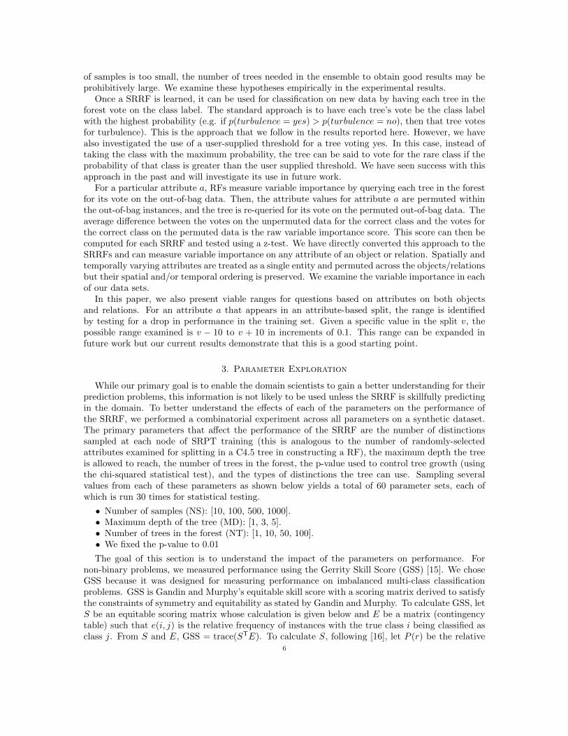
Figure 2. Schema for Points dataset: Attributes tagged <T> are temporal,<T3F> are temporal 3D fields, and untagged attributes are discrete.
frequency of class r. Using P (r) define the following:
D(n) =
1−n∑
r=1P (r)
n∑r=1
P (r), and
R(n) =1
D(n).
Let K be the number of classes and κ = 1K−1 .The elements of S are calculated as:
sn,n =κ
[n−1∑r=1
R(r) +
K−1∑r=n
D(r)
]n = (1, 2, · · · ,K)
sm,n =κ
[m−1∑r=1
R(r) +
n−1∑r=m
(−1) +
K−1∑r=n
D(r)
]1 ≤ m < K,m < n ≤ K
sn,m =sm,n 2 ≤ n ≤ K, 1 ≤ m < n
GSS varies from -1 to 1 [16]. A value of -1 indicates “intentionally” classifying incorrectly; a valueof 0 is equivalent to the performance of a random classifier; and a value of 1 indicates perfectclassification.
For the binary classification tasks, we also measure Area under the Receiver Operator Charac-teristic Curve (AUC). AUC has a long, respected history in evaluating machine learning algorithms[5, 12]. AUC measures the robustness of the classifier across the various probability thresholds [30].AUC varies from 0 to 1, with 1 indicating a perfect classifier and 0.5 indicating a random classifier.
The Points data set is a synthetic spatiotemporal relational data set that we designed to highlightthe ability of the SRRF to handle spatiotemporally varying fielded attributes. The schema for Pointsis shown in Figure 2. We generate each graph randomly according to the rules of the classes thatwe created for this data. Each graph has between 3 and a parameterized maximum number ofobjects. We varied the maximum number of objects between 5, 10 and 20, with the larger numberrepresenting more difficult problems (each graph contains more noise). Each object in the graphhas two attributes associated with it: a discrete color and a 3D-field of integers from {0, 1}. The3D-field attribute field is used to represent a point cloud with a 1 indicating a point at that locationand 0 indicating empty space. This cloud is used to represent the shape of the object. There arethree classes in the Points dataset: change, grow, and flip. Change has a box turn into a sphereand a cone turn into a cylinder. Grow has three blue spheres that grow to have a volume greaterthan ≈ 167 cubic units (radius of 40 units). Flip has a cone that flips 180 degrees along its axis. Togenerate the data, we randomly created a uniform distribution of class labels. Using the class labels,we filled in the required number of objects with the correct attributes to meet the definition of each
7
10 100 500 1000Num Samples
0.0
0.1
0.2
0.3
0.4
0.5
0.6
0.7
0.8
0.9
1.0
GSS
Points: 5 Objects: Max Depth=5.0, α=0.01
Num Treesn = 1.0 n = 10.0 n = 50.0 n = 100.0
(a) GSS by forest size
10 100 500 1000Num Samples
0.0
0.1
0.2
0.3
0.4
0.5
0.6
0.7
0.8
0.9
1.0
GSS
Points: 5 Objects: α=0.01, Num Trees=100.0
Max Depthm = 1.0 m = 3.0 m = 5.0
(b) GSS by maximum tree depth
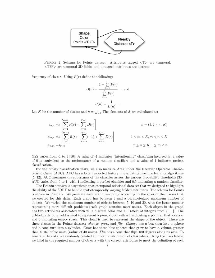
Figure 3. GSS on the synthetic points dataset with a maximum of 5 objects pergraph as a) a function of the number of trees and samples and b) a function of themaximum depth of the trees and samples.
10 100 500 1000Num Samples
0.0
0.1
0.2
0.3
0.4
0.5
0.6
0.7
0.8
0.9
1.0
GSS
Points: 10 Objects: Max Depth=5.0, α=0.01
Num Treesn = 1.0 n = 10.0 n = 50.0 n = 100.0
(a) GSS by forest size
10 100 500 1000Num Samples
0.0
0.1
0.2
0.3
0.4
0.5
0.6
0.7
0.8
0.9
1.0
GSS
Points: 10 Objects: α=0.01, Num Trees=100.0
Max Depthm = 1.0 m = 3.0 m = 5.0
(b) GSS by maximum tree depth
Figure 4. GSS on the synthetic points dataset with a maximum of 10 objects pergraph as a) a function of the number of trees and samples and b) a function of themaximum depth of the trees and samples.
class label. Additional randomly generated objects were added to the graph along with relationsthat randomly related objects within the graph. These extra objects and relations served to addnoise.
Figures 3, 4, and 5 show the performance of the SRRF on the points domain for the case of5 objects, 10 objects, and 20 objects per graph respectively. Panel a of each figure shows theperformance of the SRRF as a function of the number of trees in the forest and the number ofsamples at each level of tree growth. For panel a, the maximum depth of the tree is fixed to 5.Panel b of each figure shows the performance as a function of the maximum depth and the numberof samples. In these graphs, we fixed the number of trees at 100.
8
10 100 500 1000Num Samples
0.0
0.1
0.2
0.3
0.4
0.5
0.6
0.7
0.8
0.9
1.0
GSS
Points: 20 Objects: Max Depth=5.0, α=0.01
Num Treesn = 1.0 n = 10.0 n = 50.0 n = 100.0
(a) GSS by forest size
10 100 500 1000Num Samples
0.0
0.1
0.2
0.3
0.4
0.5
0.6
0.7
0.8
0.9
1.0
GSS
Points: 20 Objects: α=0.01, Num Trees=100.0
Max Depthm = 1.0 m = 3.0 m = 5.0
(b) GSS by maximum tree depth
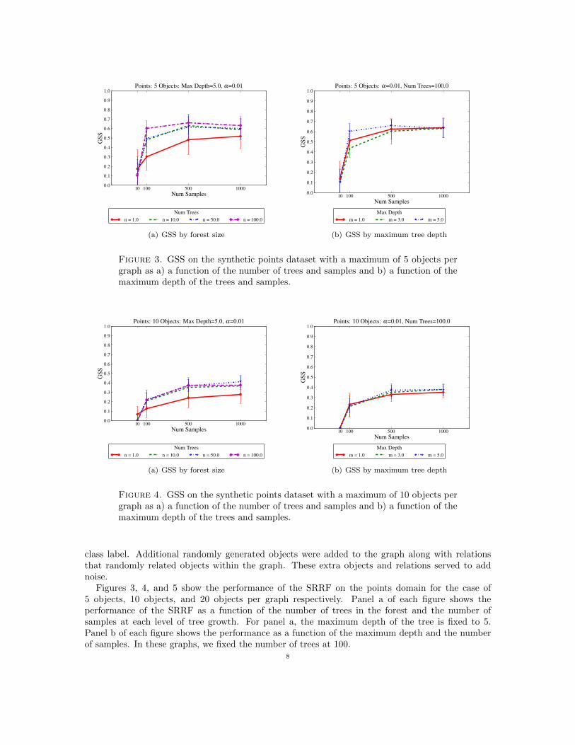
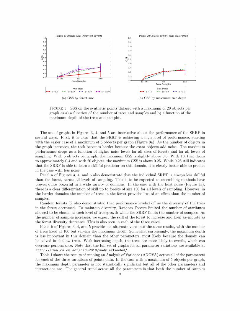
Figure 5. GSS on the synthetic points dataset with a maximum of 20 objects pergraph as a) a function of the number of trees and samples and b) a function of themaximum depth of the trees and samples.
The set of graphs in Figures 3, 4, and 5 are instructive about the performance of the SRRF inseveral ways. First, it is clear that the SRRF is achieving a high level of performance, startingwith the easier case of a maximum of 5 objects per graph (Figure 3a). As the number of objects inthe graph increases, the task becomes harder because the extra objects add noise. The maximumperformance drops as a function of higher noise levels for all sizes of forests and for all levels ofsampling. With 5 objects per graph, the maximum GSS is slightly above 0.6. With 10, that dropsto approximately 0.4 and with 20 objects, the maximum GSS is about 0.25. While 0.25 still indicatesthat the SRRF is able to learn a skillful predictor on this domain, it is clearly better able to predictin the case with less noise.
Panel a of Figures 3, 4, and 5 also demonstrate that the individual SRPT is always less skillfulthan the forest, across all levels of sampling. This is to be expected as ensembling methods haveproven quite powerful in a wide variety of domains. In the case with the least noise (Figure 3a),there is a clear differentiation of skill up to forests of size 100 for all levels of sampling. However, inthe harder domains the number of trees in the forest provides less of an effect than the number ofsamples.
Random forests [6] also demonstrated that performance leveled off as the diversity of the treesin the forest decreased. To maintain diversity, Random Forests limited the number of attributesallowed to be chosen at each level of tree growth while the SRRF limits the number of samples. Asthe number of samples increases, we expect the skill of the forest to increase and then asymptote asthe forest diversity decreases. This is also seen in each of the three cases.
Panel b of Figures 3, 4, and 5 provides an alternate view into the same results, with the numberof trees fixed at 100 but varying the maximum depth. Somewhat surprisingly, the maximum depthis less important in this domain than the other parameters, most likely because the domain canbe solved in shallow trees. With increasing depth, the trees are more likely to overfit, which candecrease performance. Note that the full set of graphs for all parameter variations are available athttp://idea.cs.ou.edu/cidu2010/sadm extended/.
Table 1 shows the results of running an Analysis of Variance (ANOVA) across all of the parametersfor each of the three variations of points data. In the case with a maximum of 5 objects per graph,the maximum depth parameter is not statistically significant but all of the other parameters andinteractions are. The general trend across all the parameters is that both the number of samples
9
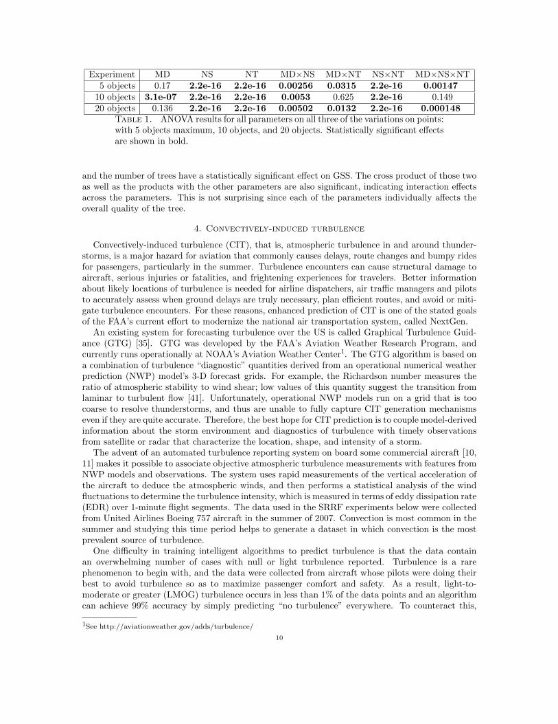
Experiment MD NS NT MD×NS MD×NT NS×NT MD×NS×NT5 objects 0.17 2.2e-16 2.2e-16 0.00256 0.0315 2.2e-16 0.00147
10 objects 3.1e-07 2.2e-16 2.2e-16 0.0053 0.625 2.2e-16 0.14920 objects 0.136 2.2e-16 2.2e-16 0.00502 0.0132 2.2e-16 0.000148
Table 1. ANOVA results for all parameters on all three of the variations on points:with 5 objects maximum, 10 objects, and 20 objects. Statistically significant effectsare shown in bold.
and the number of trees have a statistically significant effect on GSS. The cross product of those twoas well as the products with the other parameters are also significant, indicating interaction effectsacross the parameters. This is not surprising since each of the parameters individually affects theoverall quality of the tree.
4. Convectively-induced turbulence
Convectively-induced turbulence (CIT), that is, atmospheric turbulence in and around thunder-storms, is a major hazard for aviation that commonly causes delays, route changes and bumpy ridesfor passengers, particularly in the summer. Turbulence encounters can cause structural damage toaircraft, serious injuries or fatalities, and frightening experiences for travelers. Better informationabout likely locations of turbulence is needed for airline dispatchers, air traffic managers and pilotsto accurately assess when ground delays are truly necessary, plan efficient routes, and avoid or miti-gate turbulence encounters. For these reasons, enhanced prediction of CIT is one of the stated goalsof the FAA’s current effort to modernize the national air transportation system, called NextGen.
An existing system for forecasting turbulence over the US is called Graphical Turbulence Guid-ance (GTG) [35]. GTG was developed by the FAA’s Aviation Weather Research Program, andcurrently runs operationally at NOAA’s Aviation Weather Center1. The GTG algorithm is based ona combination of turbulence “diagnostic” quantities derived from an operational numerical weatherprediction (NWP) model’s 3-D forecast grids. For example, the Richardson number measures theratio of atmospheric stability to wind shear; low values of this quantity suggest the transition fromlaminar to turbulent flow [41]. Unfortunately, operational NWP models run on a grid that is toocoarse to resolve thunderstorms, and thus are unable to fully capture CIT generation mechanismseven if they are quite accurate. Therefore, the best hope for CIT prediction is to couple model-derivedinformation about the storm environment and diagnostics of turbulence with timely observationsfrom satellite or radar that characterize the location, shape, and intensity of a storm.
The advent of an automated turbulence reporting system on board some commercial aircraft [10,11] makes it possible to associate objective atmospheric turbulence measurements with features fromNWP models and observations. The system uses rapid measurements of the vertical acceleration ofthe aircraft to deduce the atmospheric winds, and then performs a statistical analysis of the windfluctuations to determine the turbulence intensity, which is measured in terms of eddy dissipation rate(EDR) over 1-minute flight segments. The data used in the SRRF experiments below were collectedfrom United Airlines Boeing 757 aircraft in the summer of 2007. Convection is most common in thesummer and studying this time period helps to generate a dataset in which convection is the mostprevalent source of turbulence.
One difficulty in training intelligent algorithms to predict turbulence is that the data containan overwhelming number of cases with null or light turbulence reported. Turbulence is a rarephenomenon to begin with, and the data were collected from aircraft whose pilots were doing theirbest to avoid turbulence so as to maximize passenger comfort and safety. As a result, light-to-moderate or greater (LMOG) turbulence occurs in less than 1% of the data points and an algorithmcan achieve 99% accuracy by simply predicting “no turbulence” everywhere. To counteract this,
1See http://aviationweather.gov/adds/turbulence/
10
10 100 500 1000Num Samples
0.0
0.1
0.2
0.3
0.4
0.5
0.6
0.7
0.8
0.9
1.0
GSS
Turbulence: α=0.01, Max Depth=5.0, Undersampled=0.0
Num Treesn = 1.0 n = 10.0 n = 50.0 n = 100.0
(a) No undersampling
10 100 500 1000Num Samples
0.0
0.1
0.2
0.3
0.4
0.5
0.6
0.7
0.8
0.9
1.0
GSS
Turbulence: α=0.01, Max Depth=5.0, Undersampled=0.7
Num Treesn = 1.0 n = 10.0 n = 50.0 n = 100.0
(b) 0.7 undersampling
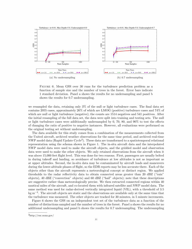
Figure 6. Mean GSS over 30 runs for the turbulence prediction problem as afunction of sample size and the number of trees in the forest. Error bars indicate1 standard deviation. Panel a shows the results for no undersampling and panel bshows the results for 0.7 undersampling.
we resampled the data, retaining only 3% of the null or light turbulence cases. The final data setcontains 2055 cases, approximately 26% of which are LMOG (positive) turbulence cases and 74% ofwhich are null or light turbulence (negative); the counts are 1514 negatives and 541 positives. Afterthe initial resampling of the full data set, the data were split into training and testing sets. The nullor light turbulence cases were additionally undersampled by 0, 70, 80, and 90% to test the effectsof changing the ratio of positive to negative instances. However, all evaluations were performed onthe original testing set without undersampling.
The data available for this study comes from a combination of the measurements collected fromthe United aircraft, archived weather observations for the same time period, and archived real-timeNWP model data (Rapid Update Cycle2). These data are transformed to a spatiotemporal relationalrepresentation using the schema shown in Figure 1. The in-situ aircraft data and the interpolatedNWP model data were used to make the aircraft objects, and the gridded model and observationdata were used to make the other objects. We only retained observations from the aircraft when itwas above 15,000 feet flight level. This was done for two reasons. First, passengers are usually beltedin during takeoff and landing, so avoidance of turbulence at low altitudes is not as important asat upper altitudes. Second, the in-situ data may be contaminated by aircraft loads and maneuversduring the lower-altitude phases of flight, so the EDR reports may be less accurate there. Each of theobjects other than the aircraft represents a meteorological concept or distinct region. We appliedthresholds to the radar reflectivity data to obtain connected areas greater than 20 dBZ (“rain”objects), 40 dBZ (“convection” objects) and 60 dBZ (“hail” objects); note that these descriptionsare suggestive rather than meteorologically precise. We then extracted connected regions within 40nautical miles of the aircraft, and co-located them with infrared satellite and NWP model data. Thesame method was used for radar-derived vertically integrated liquid (VIL), with a threshold of 3.5kg m−2. The aircraft objects are static and the observations are available only at the same time thatthe turbulence was measured. The other objects are tracked for 30 minutes, in 5 minute increments.
Figure 6 shows the GSS on an independent test set of the turbulence data as a function of thenumber of distinctions sampled and the number of trees in the forest. Panel a shows the results for noadditional undersampling and panel b shows the results for 0.7 undersampling. The undersampling
2http://ruc.noaa.gov/
11
10 100 500 1000Num Samples
0.50
0.55
0.60
0.65
0.70
0.75
0.80
0.85
0.90
0.95
1.00
AU
C
Turbulence: α=0.01, Max Depth=5.0, Undersampled=0.0
Num Treesn = 1.0 n = 10.0 n = 50.0 n = 100.0
(a) No undersampling
10 100 500 1000Num Samples
0.50
0.55
0.60
0.65
0.70
0.75
0.80
0.85
0.90
0.95
1.00
AU
C
Turbulence: α=0.01, Max Depth=5.0, Undersampled=0.7
Num Treesn = 1.0 n = 10.0 n = 50.0 n = 100.0
(b) 0.7 undersampling
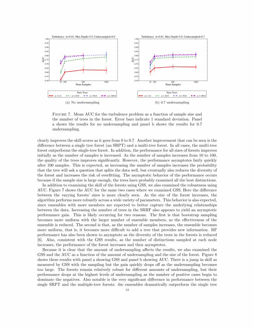
Figure 7. Mean AUC for the turbulence problem as a function of sample size andthe number of trees in the forest. Error bars indicate 1 standard deviation. Panela shows the results for no undersampling and panel b shows the results for 0.7undersampling.
clearly improves the skill scores as it goes from 0 to 0.7. Another improvement that can be seen is thedifference between a single tree forest (an SRPT) and a multi-tree forest. In all cases, the multi-treeforest outperforms the single-tree forest. In addition, the performance for all sizes of forests improvesinitially as the number of samples is increased. As the number of samples increases from 10 to 100,the quality of the trees improves significantly. However, the performance asymptotes fairly quicklyafter 100 samples. This is expected, as increasing the number of samples increases the probabilitythat the tree will ask a question that splits the data well, but eventually also reduces the diversity ofthe forest and increases the risk of overfitting. The asymptotic behavior of the performance occursbecause if the sample size is large enough, the trees have probably examined all the best distinctions.
In addition to examining the skill of the forests using GSS, we also examined the robustness usingAUC. Figure 7 shows the AUC for the same two cases where we examined GSS. Here the differencebetween the varying forests’ sizes is more clearly seen. As the size of the forest increases, thealgorithm performs more robustly across a wide variety of parameters. This behavior is also expected,since ensembles with more members are expected to better capture the underlying relationshipsbetween the data. Increasing the number of trees in the SRRF also appears to yield an asymptoticperformance gain. This is likely occurring for two reasons. The first is that bootstrap samplingbecomes more uniform with the larger number of ensemble members, so the effectiveness of theensemble is reduced. The second is that, as the number of samples increases, the ensemble becomesmore uniform, that is, it becomes more difficult to add a tree that provides new information. RFperformance has also been shown to asymptote as the diversity of the trees in the forests is reduced[6]. Also, consistent with the GSS results, as the number of distinctions sampled at each nodeincreases, the performance of the forest increases and then asymptotes.
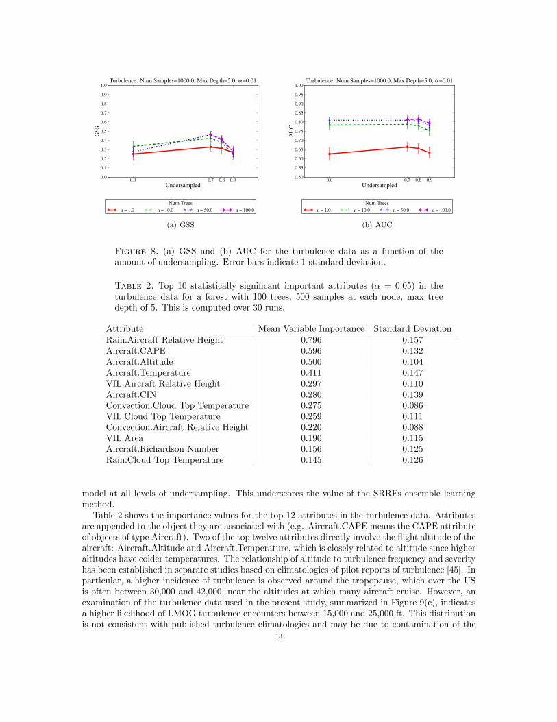
Because it is clear that the amount of undersampling affects the results, we also examined theGSS and the AUC as a function of the amount of undersampling and the size of the forest. Figure 8shows these results with panel a showing GSS and panel b showing AUC. There is a jump in skill asmeasured by GSS with the sampling but the gain quickly drops off as the undersampling becomestoo large. The forests remain relatively robust for different amounts of undersampling, but theirperformance drops at the highest levels of undersampling as the number of positive cases begin todominate the negatives. Also notable is the very significant difference in performance between thesingle SRPT and the multiple-tree forests: the ensembles dramatically outperform the single tree
12
0.0 0.7 0.8 0.9Undersampled
0.0
0.1
0.2
0.3
0.4
0.5
0.6
0.7
0.8
0.9
1.0
GSS
Turbulence: Num Samples=1000.0, Max Depth=5.0, α=0.01
Num Treesn = 1.0 n = 10.0 n = 50.0 n = 100.0
(a) GSS
0.0 0.7 0.8 0.9Undersampled
0.50
0.55
0.60
0.65
0.70
0.75
0.80
0.85
0.90
0.95
1.00
AU
C
Turbulence: Num Samples=1000.0, Max Depth=5.0, α=0.01
Num Treesn = 1.0 n = 10.0 n = 50.0 n = 100.0
(b) AUC
Figure 8. (a) GSS and (b) AUC for the turbulence data as a function of theamount of undersampling. Error bars indicate 1 standard deviation.
Table 2. Top 10 statistically significant important attributes (α = 0.05) in theturbulence data for a forest with 100 trees, 500 samples at each node, max treedepth of 5. This is computed over 30 runs.
Attribute Mean Variable Importance Standard DeviationRain.Aircraft Relative Height 0.796 0.157Aircraft.CAPE 0.596 0.132Aircraft.Altitude 0.500 0.104Aircraft.Temperature 0.411 0.147VIL.Aircraft Relative Height 0.297 0.110Aircraft.CIN 0.280 0.139Convection.Cloud Top Temperature 0.275 0.086VIL.Cloud Top Temperature 0.259 0.111Convection.Aircraft Relative Height 0.220 0.088VIL.Area 0.190 0.115Aircraft.Richardson Number 0.156 0.125Rain.Cloud Top Temperature 0.145 0.126
model at all levels of undersampling. This underscores the value of the SRRFs ensemble learningmethod.
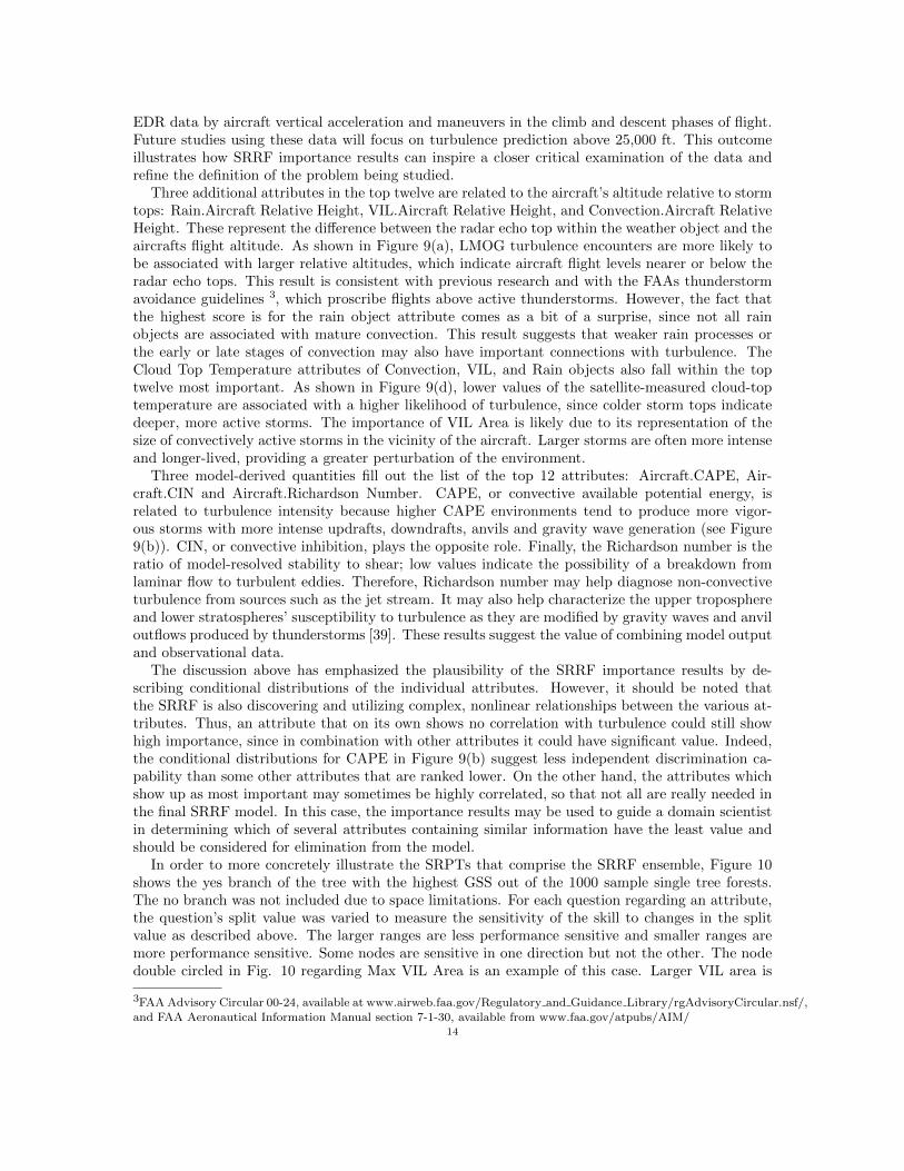
Table 2 shows the importance values for the top 12 attributes in the turbulence data. Attributesare appended to the object they are associated with (e.g. Aircraft.CAPE means the CAPE attributeof objects of type Aircraft). Two of the top twelve attributes directly involve the flight altitude of theaircraft: Aircraft.Altitude and Aircraft.Temperature, which is closely related to altitude since higheraltitudes have colder temperatures. The relationship of altitude to turbulence frequency and severityhas been established in separate studies based on climatologies of pilot reports of turbulence [45]. Inparticular, a higher incidence of turbulence is observed around the tropopause, which over the USis often between 30,000 and 42,000, near the altitudes at which many aircraft cruise. However, anexamination of the turbulence data used in the present study, summarized in Figure 9(c), indicatesa higher likelihood of LMOG turbulence encounters between 15,000 and 25,000 ft. This distributionis not consistent with published turbulence climatologies and may be due to contamination of the
13
EDR data by aircraft vertical acceleration and maneuvers in the climb and descent phases of flight.Future studies using these data will focus on turbulence prediction above 25,000 ft. This outcomeillustrates how SRRF importance results can inspire a closer critical examination of the data andrefine the definition of the problem being studied.
Three additional attributes in the top twelve are related to the aircraft’s altitude relative to stormtops: Rain.Aircraft Relative Height, VIL.Aircraft Relative Height, and Convection.Aircraft RelativeHeight. These represent the difference between the radar echo top within the weather object and theaircrafts flight altitude. As shown in Figure 9(a), LMOG turbulence encounters are more likely tobe associated with larger relative altitudes, which indicate aircraft flight levels nearer or below theradar echo tops. This result is consistent with previous research and with the FAAs thunderstormavoidance guidelines 3, which proscribe flights above active thunderstorms. However, the fact thatthe highest score is for the rain object attribute comes as a bit of a surprise, since not all rainobjects are associated with mature convection. This result suggests that weaker rain processes orthe early or late stages of convection may also have important connections with turbulence. TheCloud Top Temperature attributes of Convection, VIL, and Rain objects also fall within the toptwelve most important. As shown in Figure 9(d), lower values of the satellite-measured cloud-toptemperature are associated with a higher likelihood of turbulence, since colder storm tops indicatedeeper, more active storms. The importance of VIL Area is likely due to its representation of thesize of convectively active storms in the vicinity of the aircraft. Larger storms are often more intenseand longer-lived, providing a greater perturbation of the environment.
Three model-derived quantities fill out the list of the top 12 attributes: Aircraft.CAPE, Air-craft.CIN and Aircraft.Richardson Number. CAPE, or convective available potential energy, isrelated to turbulence intensity because higher CAPE environments tend to produce more vigor-ous storms with more intense updrafts, downdrafts, anvils and gravity wave generation (see Figure9(b)). CIN, or convective inhibition, plays the opposite role. Finally, the Richardson number is theratio of model-resolved stability to shear; low values indicate the possibility of a breakdown fromlaminar flow to turbulent eddies. Therefore, Richardson number may help diagnose non-convectiveturbulence from sources such as the jet stream. It may also help characterize the upper troposphereand lower stratospheres’ susceptibility to turbulence as they are modified by gravity waves and anviloutflows produced by thunderstorms [39]. These results suggest the value of combining model outputand observational data.
The discussion above has emphasized the plausibility of the SRRF importance results by de-scribing conditional distributions of the individual attributes. However, it should be noted thatthe SRRF is also discovering and utilizing complex, nonlinear relationships between the various at-tributes. Thus, an attribute that on its own shows no correlation with turbulence could still showhigh importance, since in combination with other attributes it could have significant value. Indeed,the conditional distributions for CAPE in Figure 9(b) suggest less independent discrimination ca-pability than some other attributes that are ranked lower. On the other hand, the attributes whichshow up as most important may sometimes be highly correlated, so that not all are really needed inthe final SRRF model. In this case, the importance results may be used to guide a domain scientistin determining which of several attributes containing similar information have the least value andshould be considered for elimination from the model.
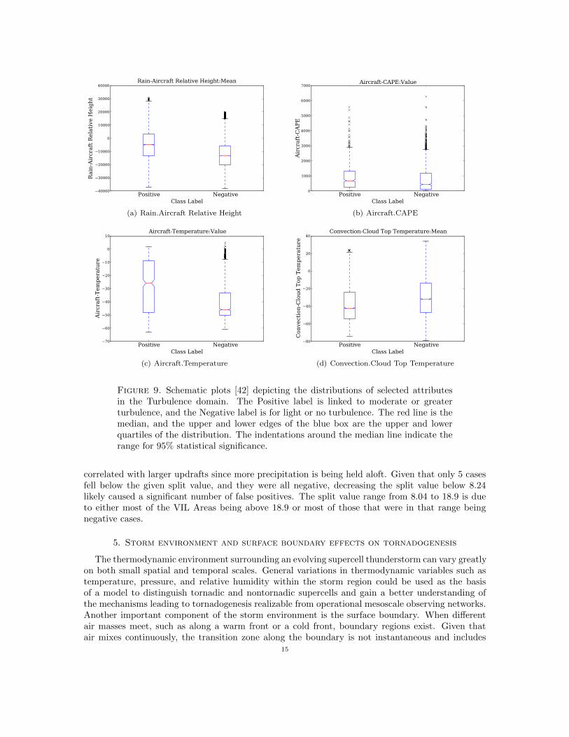
In order to more concretely illustrate the SRPTs that comprise the SRRF ensemble, Figure 10shows the yes branch of the tree with the highest GSS out of the 1000 sample single tree forests.The no branch was not included due to space limitations. For each question regarding an attribute,the question’s split value was varied to measure the sensitivity of the skill to changes in the splitvalue as described above. The larger ranges are less performance sensitive and smaller ranges aremore performance sensitive. Some nodes are sensitive in one direction but not the other. The nodedouble circled in Fig. 10 regarding Max VIL Area is an example of this case. Larger VIL area is
3FAA Advisory Circular 00-24, available at www.airweb.faa.gov/Regulatory and Guidance Library/rgAdvisoryCircular.nsf/,
and FAA Aeronautical Information Manual section 7-1-30, available from www.faa.gov/atpubs/AIM/14
Positive NegativeClass Label
40000
30000
20000
10000
0
10000
20000
30000
40000R
ain
-Air
craft
Rela
tive
Heig
ht
Rain-Aircraft Relative Height:Mean
(a) Rain.Aircraft Relative Height
Positive NegativeClass Label
0
1000
2000
3000
4000
5000
6000
7000
Air
craft
-CA
PE
Aircraft-CAPE:Value
(b) Aircraft.CAPE
Positive NegativeClass Label
70
60
50
40
30
20
10
0
10
Air
craft
-Tem
pera
ture
Aircraft-Temperature:Value
(c) Aircraft.Temperature
Positive NegativeClass Label
80
60
40
20
0
20
40
Con
vect
ion
-Clo
ud
Top
Tem
pera
ture
Convection-Cloud Top Temperature:Mean
(d) Convection.Cloud Top Temperature
Figure 9. Schematic plots [42] depicting the distributions of selected attributesin the Turbulence domain. The Positive label is linked to moderate or greaterturbulence, and the Negative label is for light or no turbulence. The red line is themedian, and the upper and lower edges of the blue box are the upper and lowerquartiles of the distribution. The indentations around the median line indicate therange for 95% statistical significance.
correlated with larger updrafts since more precipitation is being held aloft. Given that only 5 casesfell below the given split value, and they were all negative, decreasing the split value below 8.24likely caused a significant number of false positives. The split value range from 8.04 to 18.9 is dueto either most of the VIL Areas being above 18.9 or most of those that were in that range beingnegative cases.
5. Storm environment and surface boundary effects on tornadogenesis
The thermodynamic environment surrounding an evolving supercell thunderstorm can vary greatlyon both small spatial and temporal scales. General variations in thermodynamic variables such astemperature, pressure, and relative humidity within the storm region could be used as the basisof a model to distinguish tornadic and nontornadic supercells and gain a better understanding ofthe mechanisms leading to tornadogenesis realizable from operational mesoscale observing networks.Another important component of the storm environment is the surface boundary. When differentair masses meet, such as along a warm front or a cold front, boundary regions exist. Given thatair mixes continuously, the transition zone along the boundary is not instantaneous and includes
15
Is the median aircraft relative height with respect to a rain object >= 1299 ft?
Range=(-1309, -1289)
Is the median coverage attribute on the relation between rain and VIL
objects >= 0.1? Range = (0.1, 0.1)
Is the Richardson Number on the aircraft object <= -4.75?
Range=(-7.05, -2.55)
Are there >=13 rain objects?
Is the aircraft temperature < -20
degrees C? Range=(-30.0,-16.1)
Is the aircraft altitude < 36,708 ft? Range=(36698,36708)
P(T) = 0.06 P(T) =0.55
P(T) = 0.82
P(T) = 0.0
Is the Max VIL Area > 9.04? Range=
(8.24,18.9)
P(T) = 0.70 P(T) = 0.0
Is the mean relative height between a rain object and aircraft > 4919 ft? Range=(4909, 4929)
Is the mean reflectivity of the hail object > 62.3 dBZ?Range=(52.3,72.3)
P(T)=0.33Is the standard
deviation of the rain reflectivity > 0.3?Range=(0,2.3)?
Are there at least 10 instances of convection objects containing VIL?
P(T) = 0.96 P(T) = 0.77
P(T) = 0.47
Are there at least 2 nearby relations between aircraft
and VIL with a max azimuth > 106.0?
P(T) = 0.83Is the aircraft's
Richardson number < -17.54? Range=
(-27.54,-7.64)
P(T) = 0.78Is the aircraft CAPE <
1798 J/kg?Range=(1788,1798)
P(T) = 0.13 P(T) = 0.75
Subtree removed for space
Y (16) N (11)
Y (27)N (17)
Y (44)N (15)
Y (59)
Y (50) N (5)
N (55)
Y (114)
Y (9)
Y (52) N (100)
Y (152)N (15)
N (167)
Y (176)
Y (18)
Y (9)
Y (23) N (4)
N (27)
N (36)
N (54)
N (230)
Y (344) N (156)
Figure 10. Left most subtree of the most highly ranked SRPT from the turbulencedomain for 1000 samples. The tree shows the ranges on the attribute questions. Dueto space limitations, we focused on the left-most subtree. The node that is doublecircled is discussed in the text. P(T) denotes the probability of a LMOG turbulenceevent.
regions of strong temperature and moisture gradients. In addition to fronts, boundaries also occuralong drylines or due to outflow from thunderstorms. While boundaries are commonly associatedwith the generation of storms through the lifting of warm, moist air over cool, dry air, their overallimpact on the generation of tornadoes is not well understood. Markowski et al. [22] describe howboundaries can yield a zone of enhanced horizontal rotation. A supercell thunderstorm with a strongupdraft moving through the zone can vertically tilt and stretch the enhanced horizontal rotationwhich assists with the process of producing a tornado. That study analyzed strong tornadic super-cell thunderstorms over a one-year period and found that 70% occurred near frontal boundaries.However, due to the limited sample size and time period, further study was needed to quantify therelationship between boundaries and tornadoes over longer periods.
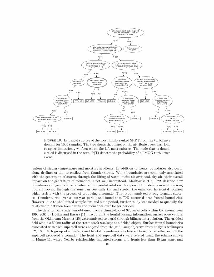
The data for our study was obtained from a climatology of 926 supercells within Oklahoma from1994-2003 by Hocker and Basara [17]. To obtain the frontal passage information, surface observationsfrom the Oklahoma Mesonet [25] were analyzed to a grid through bilinear interpolation. The griddedfield within a 50 km radius of the storm track was kept as a fielded object. Surface frontal boundariesassociated with each supercell were analyzed from the grid using objective front analysis techniques[32, 18]. Each group of supercells and frontal boundaries was labeled based on whether or not thesupercell produced a tornado. The front and supercell data were related using the schema shownin Figure 11, where Nearby relationships indicated storms and fronts less than 40 km apart and
16
StormRain <T>
Wind Direction <T>Wind DSD* <T>Wind SSD* <T>
Dew Point Temperature <T2F>Air Temperature <T2F>
Relative Humidity <T2F>Pressure <T2F>LCLH* <T2F>
ThetaE* <T2F>Wind <T2VF>
Bearing <T>Azimuth <T>Range <T>Height <T>
Reflectivity <T>Latitude <T>
Longitude <T>Total Displacement <T>
Step Distance Traveled <T>Turn Angle <T>
Previous Bearing <T>
NearbyDistance <T>
*Abbreviations Wind DSD: Wind Direction Standard Deviation Wind SSD: Wind Speed Standard Deviation LCLH: Height of the Lifted Condensation Level TFP: Thermal Front Parameter ThetaE*: Equivalent Potential Temperature
FrontCenter X <T>Center Y <T>
Area <T>Eccentricity <T>
Major Axis Length <T>Minor Axis Length <T>
Oriented <T>ThetaE* <T2F>
Air Temperature <T2F>TFP* <T2F>
Dew Point Temperature <T2F>LCLH* <T2F>
Pressure <T2F>Wind <T2VF>
On Top OfDistance <T>
Figure 11. Schema for tornadogenesis data. Temporal data is denoted with a<T> and 2-dimensional fielded data with a <T2F>.
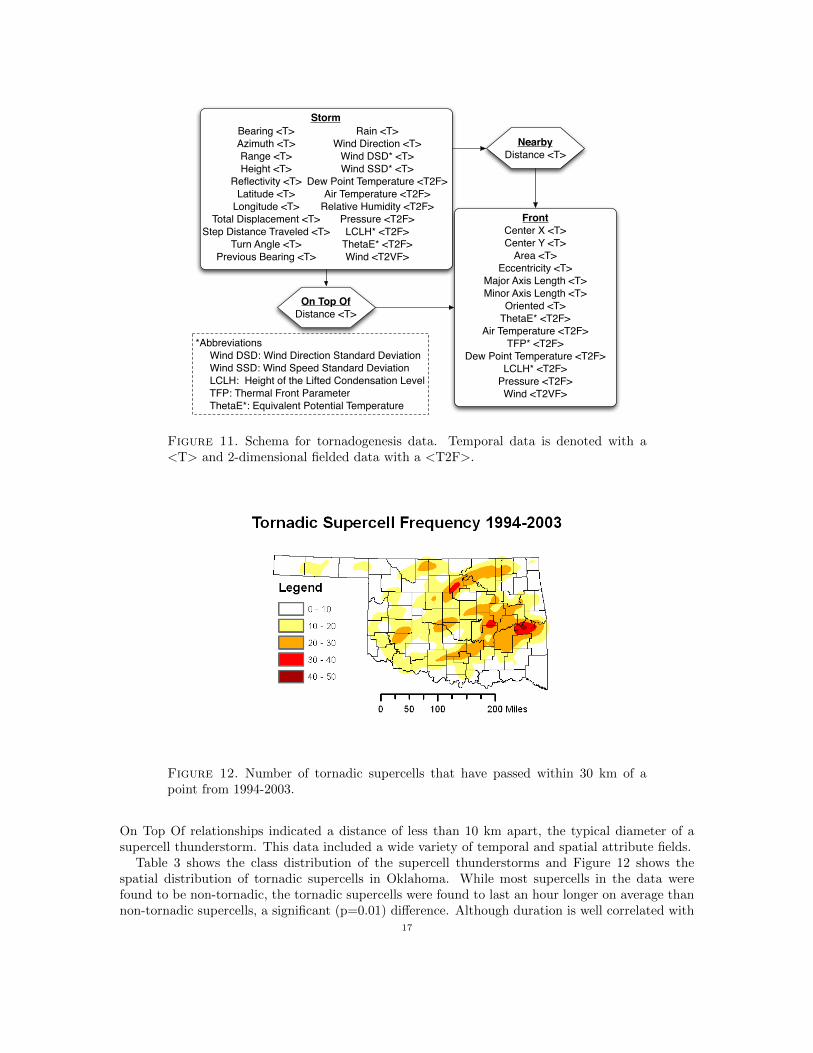
Figure 12. Number of tornadic supercells that have passed within 30 km of apoint from 1994-2003.
On Top Of relationships indicated a distance of less than 10 km apart, the typical diameter of asupercell thunderstorm. This data included a wide variety of temporal and spatial attribute fields.
Table 3 shows the class distribution of the supercell thunderstorms and Figure 12 shows thespatial distribution of tornadic supercells in Oklahoma. While most supercells in the data werefound to be non-tornadic, the tornadic supercells were found to last an hour longer on average thannon-tornadic supercells, a significant (p=0.01) difference. Although duration is well correlated with
17
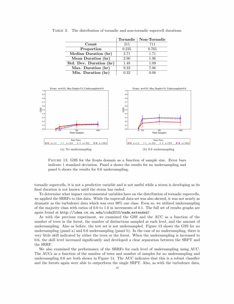
Table 3. The distribution of tornadic and non-tornadic supercell durations.
Tornadic Non-TornadicCount 215 711
Proportion 0.235 0.765Median Duration (hr) 2.71 1.71Mean Duration (hr) 2.90 1.96
Std. Dev. Duration (hr) 1.48 1.09Max. Duration (hr) 9.33 7.06Min. Duration (hr) 0.32 0.08
10 100 500 1000Num Samples
0.0
0.1
0.2
0.3
0.4
0.5
0.6
0.7
0.8
0.9
1.0
GSS
Fronts: α=0.01, Max Depth=5.0, Undersampled=0.0
Num Treesn = 1.0 n = 10.0 n = 50.0 n = 100.0
(a) No undersampling
10 100 500 1000Num Samples
0.0
0.1
0.2
0.3
0.4
0.5
0.6
0.7
0.8
0.9
1.0
GSS
Fronts: α=0.01, Max Depth=5.0, Undersampled=0.6
Num Treesn = 1.0 n = 10.0 n = 50.0 n = 100.0
(b) 0.6 undersampling
Figure 13. GSS for the fronts domain as a function of sample size. Error barsindicate 1 standard deviation. Panel a shows the results for no undersampling andpanel b shows the results for 0.6 undersampling.
tornadic supercells, it is not a predictive variable and is not useful while a storm is developing as itsfinal duration is not known until the storm has ended.
To determine what impact environmental variables have on the distribution of tornadic supercells,we applied the SRRFs to this data. While the supercall data set was also skewed, it was not nearly asdramatic as the turbulence data which was over 99% one class. Even so, we utilized undersamplingof the majority class with ratios of 0.0 to 1.0 in increments of 0.1. The full set of results graphs areagain found at http://idea.cs.ou.edu/cidu2010/sadm extended/.
As with the previous experiment, we examined the GSS and the AUC as a function of thenumber of trees in the forest, the number of distinctions sampled at each level, and the amount ofundersampling. Also as before, the test set is not undersampled. Figure 13 shows the GSS for noundersampling (panel a) and 0.6 undersampling (panel b). In the case of no undersampling, there isvery little skill indicated by either the trees or the forest. When the undersampling is increased to0.6, the skill level increased significantly and developed a clear separation between the SRPT andthe SRRF.
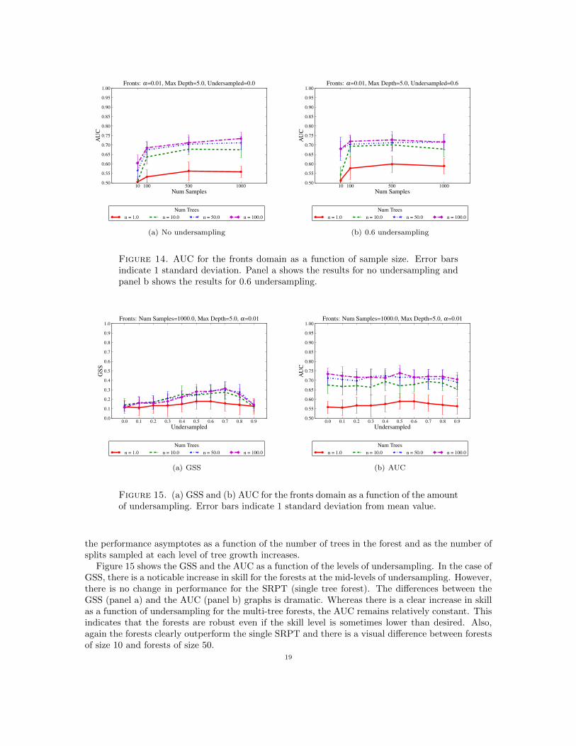
We also examined the performance of the SRRFs for each level of undersampling using AUC.The AUCs as a function of the number of trees and number of samples for no undersampling andundersampling 0.6 are both shown in Figure 14. The AUC indicates that this is a robust classifierand the forests again were able to outperform the single SRPT. Also, as with the turbulence data,
18
10 100 500 1000Num Samples
0.50
0.55
0.60
0.65
0.70
0.75
0.80
0.85
0.90
0.95
1.00
AU
C
Fronts: α=0.01, Max Depth=5.0, Undersampled=0.0
Num Treesn = 1.0 n = 10.0 n = 50.0 n = 100.0
(a) No undersampling
10 100 500 1000Num Samples
0.50
0.55
0.60
0.65
0.70
0.75
0.80
0.85
0.90
0.95
1.00
AU
C
Fronts: α=0.01, Max Depth=5.0, Undersampled=0.6
Num Treesn = 1.0 n = 10.0 n = 50.0 n = 100.0
(b) 0.6 undersampling
Figure 14. AUC for the fronts domain as a function of sample size. Error barsindicate 1 standard deviation. Panel a shows the results for no undersampling andpanel b shows the results for 0.6 undersampling.
0.0 0.1 0.2 0.3 0.4 0.5 0.6 0.7 0.8 0.9Undersampled
0.0
0.1
0.2
0.3
0.4
0.5
0.6
0.7
0.8
0.9
1.0
GSS
Fronts: Num Samples=1000.0, Max Depth=5.0, α=0.01
Num Treesn = 1.0 n = 10.0 n = 50.0 n = 100.0
(a) GSS
0.0 0.1 0.2 0.3 0.4 0.5 0.6 0.7 0.8 0.9Undersampled
0.50
0.55
0.60
0.65
0.70
0.75
0.80
0.85
0.90
0.95
1.00
AU
C
Fronts: Num Samples=1000.0, Max Depth=5.0, α=0.01
Num Treesn = 1.0 n = 10.0 n = 50.0 n = 100.0
(b) AUC
Figure 15. (a) GSS and (b) AUC for the fronts domain as a function of the amountof undersampling. Error bars indicate 1 standard deviation from mean value.
the performance asymptotes as a function of the number of trees in the forest and as the number ofsplits sampled at each level of tree growth increases.
Figure 15 shows the GSS and the AUC as a function of the levels of undersampling. In the case ofGSS, there is a noticable increase in skill for the forests at the mid-levels of undersampling. However,there is no change in performance for the SRPT (single tree forest). The differences between theGSS (panel a) and the AUC (panel b) graphs is dramatic. Whereas there is a clear increase in skillas a function of undersampling for the multi-tree forests, the AUC remains relatively constant. Thisindicates that the forests are robust even if the skill level is sometimes lower than desired. Also,again the forests clearly outperform the single SRPT and there is a visual difference between forestsof size 10 and forests of size 50.
19
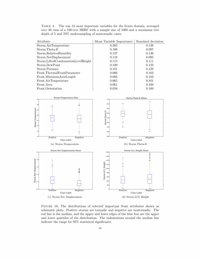
Table 4. The top 12 most important variables for the fronts domain, averagedover 30 runs of a 100-tree SRRF with a sample size of 1000 and a maximum treedepth of 5 and 70% undersampling of nontornadic cases.
Attribute Mean Variable Importance Standard deviationStorm.AirTemperature 0.283 0.138Storm.Theta-E 0.198 0.097Storm.RelativeHumidity 0.137 0.146Storm.NetDisplacement 0.118 0.095Storm.LiftedCondensationLevelHeight 0.115 0.111Storm.DewPoint 0.109 0.123Storm.Pressure 0.101 0.128Front.ThermalFrontParameter 0.066 0.103Front.MinimumAxisLength 0.066 0.103Front.AirTemperature 0.065 0.101Front.Area 0.061 0.100Front.Orientation 0.058 0.100
Positive NegativeClass Label
10
15
20
25
30
35
40
45
Sto
rm-T
em
pera
ture
Storm-Temperature:Max
(a) Storm.Temperature
Positive NegativeClass Label
290
300
310
320
330
340
350
360
370
Sto
rm-T
heta
-E
Storm-Theta-E:Mean
(b) Storm.Theta-E
Positive NegativeClass Label
0.0
0.5
1.0
1.5
2.0
2.5
Sto
rm-N
et
Dis
pla
cem
en
t
Storm-Net Displacement:Mean
(c) Storm.Net Displacement
Positive NegativeClass Label
0
200
400
600
800
1000
1200
1400
1600
1800
Sto
rm-L
CL
Heig
ht
Storm-LCL Height:Mean
(d) Storm.LCL Height
Figure 16. The distributions of selected important front attributes shown asschematic plots. Positive storms are tornadic and negative are nontornadic. Thered line is the median, and the upper and lower edges of the blue box are the upperand lower quartiles of the distribution. The indentations around the median lineindicate the range for 95% statistical significance.
20
To understand which variables are the most important in determining whether a supercell istornadic, we calculated the variable importance for the resampled data, as shown in Table 4. Sevenof the top twelve variables were associated with the storm only, indicating that characteristics ofthe storm environment are generally more influential than conditions along surrounding boundaries.Air temperature, equivalent potential temperature (theta-e), and relative humidity were the mostimportant variables. For a greater understanding of why some of these variables are important, weproduced schematic plots [42] that visually compare the medians, upper and lower quartiles, and fullrange of the distributions for both types of storms (Fig. 16). Although the distributions for the meanand maximum values of temperature, theta-e, and relative humidity were similar for tornadic andnontornadic storms, the medians of those quantities were significantly higher for tornadic storms(Fig. 16). In general, warmer and more moist environments tend to be more unstable therebyenhancing the potential for tornadic storms. Net displacement is significantly higher for tornadicstorms (Fig. 16(c)) and is tied to the duration of the storm, which is consistent with the findingsof [8] that long duration supercells are more likely to be tornadic. Storm pressure is related to theintensity of the storm. Lifted Condensation Level (LCL) Height estimates the distance from thecloud base to the ground and is proportional to the dew point depression. Bunkers [8] and othershave shown that lower LCL heights are associated with weaker downdrafts and cold pools, leadingto longer-lasting supercell storms and more favorable environments for tornadoes. In the dataset,the mean LCL heights distribution was more concentrated in the lower values for tornadic supercells(Fig. 16(d)) although the medians were not significantly different. As shown by the selection ofimportant variables, the SRRF confirms trends discussed in the literature.
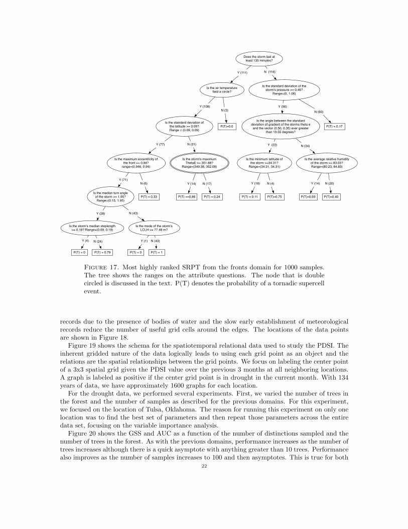
Figure 17 shows the tree with the highest GSS on the training set in the 1000 sample single-tree forests. Because it is difficult to fit even a single tree on the page, we focused only on thesingle-tree forests for this figure. Each of the attribute questions show the viable range for thatsplit. For example, the double circled node splits the data by asking “Is the storm’s maximumThetaE ≥ 351.88?” The range for this split [349.38, 352.08], which means that ThetaE can varyby about ±2 and the performance of the tree will remain the same. In a physical context, thetree is capturing the potential breakpoint for a critical thermodynamic variable associated withintense convective thunderstorms. ThetaE is a conserved thermodynamic quantity that takes intoaccount the combined temperature and moisture properties of the atmosphere. As ThetaE increases,the potential instability of the atmosphere increases and the likelihood of intense convection alsoincreases. For this study, the value of 351.88 yields a node that identifies significantly greateroccurrences of tornadic supercells given the observed values of ThetaE which further reinforcesthe notion that surface-based observations can yield predictive skill in identifying environmentalconditions that can differentiate between tornadic an non-tornadic storms.
6. Drought
Drought, loosely defined as insufficient water for normal purposes, has one of the highest costs ofany natural event in terms of socioeconomic loss. In the United States alone, drought has cost theeconomy over $5B annually on average since 1980 and extreme drought events rival hurricanes intheir destructive potential [21]. Although drought differs significantly from the previous applicationdomains, the impact demonstrates that there is a need for an improved understanding of drought.One of the interesting differences for SRRFs is that drought acts on a much slower temporal andmuch wider spatial scale.
The geographical extent of our drought analysis roughly corresponds to the Southern Great Plainsof the United States. Because we have previously demonstrated [9] that the Palmer Drought SeverityIndex (PDSI) exhibits strong spatial and temporal structure in terms of its predictability, we continueto focus on the PDSI data. The PDSI drought data is provided on a 2.5 degree geographic coordinategrid and each coordinate has 134 years of data recorded in one month intervals4. Incomplete data
4http://iridl.ldeo.columbia.edu/
21
Does the storm last at least 135 minutes?
Is the air temperature field a circle?
Is the standard deviation of the latitude >= 0.09?Range = (0.09, 0.09)
Is the maximum eccentricity of the front >= 0.94?
range=(0.946, 0.94)
Is the median turn angle of the storm >= 1.95?Range=(0.15, 1.95)
Is the storm's median steplength >= 0.19? Range=(0.09, 0.19)
P(T) = 0 P(T) = 0.79
Is the mode of the storm's LCLH >= 77.48 m?
P(T) = 0 P(T) = 1
P(T) = 0.33
Is the storm's maximum ThetaE >= 351.88?
Range=(349.38, 352.08)
P(T) ==0.86 P(T) = 0.24
P(T)=0.0
Is the standard deviation of the storm's pressure >= 0.46?
Range=(0, 1.06)
Is the angle between the standard deviation of gradient of the storms theta e and the vector (0.50, 0.35) ever greater
than 19.55 degrees?
Is the minimum latitude of the storm >=34.31?
Range=(34.31, 34.31)
P(T) = 0.11 P(T)=0.75
Is the average relative humidify of the storm >= 83.03?Range=(80.23, 84.83)
P(T)=0.93 P(T)=0.40
P(T) = 0.17
Y (4) N (24)
Y (28)
Y (1) N (43)
N (43)
Y (71)N (6)
Y (77)
Y (14) N (17)
N (31)
Y (108) N (3)
Y (18) N (4)
Y (22)
Y (14) N (20)
N (34)
Y (56)N (60)
N (116)Y (111)
Figure 17. Most highly ranked SRPT from the fronts domain for 1000 samples.The tree shows the ranges on the attribute questions. The node that is doublecircled is discussed in the text. P(T) denotes the probability of a tornadic supercellevent.
records due to the presence of bodies of water and the slow early establishment of meteorologicalrecords reduce the number of useful grid cells around the edges. The locations of the data pointsare shown in Figure 18.
Figure 19 shows the schema for the spatiotemporal relational data used to study the PDSI. Theinherent gridded nature of the data logically leads to using each grid point as an object and therelations are the spatial relationships between the grid points. We focus on labeling the center pointof a 3x3 spatial grid given the PDSI value over the previous 3 months at all neighboring locations.A graph is labeled as positive if the center grid point is in drought in the current month. With 134years of data, we have approximately 1600 graphs for each location.
For the drought data, we performed several experiments. First, we varied the number of trees inthe forest and the number of samples as described for the previous domains. For this experiment,we focused on the location of Tulsa, Oklahoma. The reason for running this experiment on only onelocation was to find the best set of parameters and then repeat those parameters across the entiredata set, focusing on the variable importance analysis.
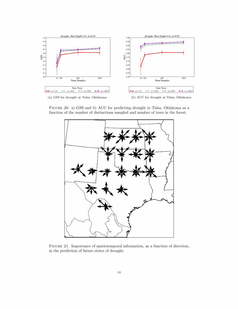
Figure 20 shows the GSS and AUC as a function of the number of distinctions sampled and thenumber of trees in the forest. As with the previous domains, performance increases as the number oftrees increases although there is a quick asymptote with anything greater than 10 trees. Performancealso improves as the number of samples increases to 100 and then asymptotes. This is true for both
22
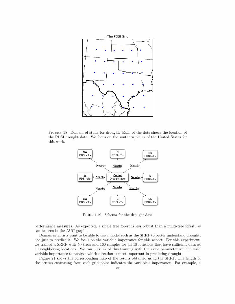
Figure 18. Domain of study for drought. Each of the dots shows the location ofthe PDSI drought data. We focus on the southern plains of the United States forthis work.
NWPDSI <T>
SWPDSI <T>
WPDSI <T>
NEPDSI <T>
NPDSI <T>
SPDSI <T>
SEPDSI <T>
EPDSI <T>
CenterDrought label
Nearby
Nearby Nearby Nearby
Nearby Nearby
NearbyNearby
Figure 19. Schema for the drought data
performance measures. As expected, a single tree forest is less robust than a multi-tree forest, ascan be seen in the AUC graph.
Domain scientists want to be able to use a model such as the SRRF to better understand drought,not just to predict it. We focus on the variable importance for this aspect. For this experiment,we trained a SRRF with 50 trees and 100 samples for all 18 locations that have sufficient data atall neighboring locations. We ran 30 runs of this training with the same parameter set and usedvariable importance to analyze which direction is most important in predicting drought.
Figure 21 shows the corresponding map of the results obtained using the SRRF. The length ofthe arrows emanating from each grid point indicates the variable’s importance. For example, a
23
10 100 500 1000Num Samples
0.0
0.1
0.2
0.3
0.4
0.5
0.6
0.7
0.8
0.9
1.0
GSS
drought: Max Depth=5.0, α=0.01
Num Treesn = 1.0 n = 10.0 n = 50.0 n = 100.0
(a) GSS for drought at Tulsa, Oklahoma
10 100 500 1000Num Samples
0.50
0.55
0.60
0.65
0.70
0.75
0.80
0.85
0.90
0.95
1.00
AU
C
drought: Max Depth=5.0, α=0.01
Num Treesn = 1.0 n = 10.0 n = 50.0 n = 100.0
(b) AUC for drought at Tulsa, Oklahoma
Figure 20. a) GSS and b) AUC for predicting drought in Tulsa, Oklahoma as afunction of the number of distinctions sampled and number of trees in the forest.
Figure 21. Importance of spatiotemporal information, as a function of direction,in the prediction of future states of drought.
24
long arrow pointing towards the southeast would indicate that spatiotemporal information to thesoutheast of the center grid point is more useful in predicting the future occurrence of drought inthe center than a direction that exhibited a lower variable importance (shorter arrow).
It is immediately seen that spatiotemporal structure exists in the abilities of the various cardinaland inter-cardinal directions to predict the presence of drought at the center grid points. Thishighlights the potential ability of the SRRF algorithm to aid in drought response planning andmitigation over short time spans. However, not only does Figure 21 demonstrate the ability topredict, it also begins to hint at geographic structure with regards to how drought responds toits spatiotemporal informational surroundings. This is most clearly seen from the similarity ofthe rosettes of variable importance surrounding the sites in Eastern and Central Kansas. Theirqualitative similarity is suggestive that drought behaves similarly across this geographic region.Other potential regions may be seen in the Western Oklahoma/Northern Texas Panhandle, and inthe Southeastern New Mexico/Southern Texas Panhandle rosettes.
Our results are encouraging and warrant further investigation into the strength of the similaritybetween rosettes, the inclusion of seasonality into the study, and the variations that drought indicesdifferent from the PDSI might present. And finally, as nearly all geographic regions exhibit indi-vidualized behavior, rather than relying upon Tulsa to calibrate the experimental parameters, eachgrid cell should be examined for its own set of “best parameters.”
7. Conclusions
We have introduced and validated a significantly augmented Spatiotemporal Relational RandomForest, a new Random Forest based algorithm that learns with spatiotemporally varying relationaldata. We have focused our application of the SRRF algorithm on three real-world severe weatherdomains: turbulence, tornadoes and drought. In each domain, we demonstrated that the SRRF is astrong predictor and that the variable importance analysis significantly aids human understandingof the results. The contributions of this paper include the enhanced SRRF algorithm, the variableimportance analysis for spatiotemporally varying relational data, the enhancements of the underlyingSRPT, parameter exploration, and a thorough validation on real-world severe weather data.
The current FAA turbulence prediction algorithm, GTG [35], is based primarily on NWP modeldata, though efforts are underway to integrate observations to better diagnose convective turbulence[44]. We anticipate that the SRRF will aid in this improvement by uncovering new spatiotemporalrelationships with predictive value via the variable importance analyses. Furthermore, to evaluateits potential to become a useful component of the prediction algorithm, we are evaluating griddedpredictions made by the SRRF on case studies drawn from selected days. We hope to integrate theSRRF into the next-generation turbulence prediction product.
Our work in the tornado domain is a piece of a larger project focusing on understanding theformation of tornadoes through high resolution simulations as well as the analysis of observationaldata. Future work on this same 10-year climatological data set includes extending the time period,extending the period before each storm, and expanding the set of environmental variables. Allof our work on tornadoes will also be immediately relevant for the Warn-on-Forecast models beingdeveloped for the National Weather Service. Our study of a 10 year dataset of tornadoes in Oklahomais helping to better understand “what” atmospheric variables are critical “when.” This provides basicnew insights into the overall set of processes related to the occurrence of tornadic supercells. In thefuture, this will be integrated with the knowledge gained through field studies such as VORTEX 25.
Our drought application is also a piece of a larger project studying the predictability of drought inthe continental United States using a variety of data mining techniques. The goal of this project isto improve our understanding of how drought moves and thus to improve the predictions of drought,enabling those affected by it to mitigate the impact.
5http://www.vortex2.org/home/
25
Our long term goals include integration of the SRRF and/or the knowledge gained from the SRRFinto current prediction algorithms. As part of this, we need to demonstrate that our algorithms areskillful in whatever way that skill is measured for each domain and we need to compare to existingalgorithms. For tornadoes, skill is most often measured using probability of detection (POD) andfalse alarm ratio (FAR) but there is not an a-priori level of POD/FAR or AUC/GSS such that analgorithm can be automatically used to issue tornado warnings. Studies such as [7] indicate thatthese may not even be the best skill measures to use. Currently, tornado warnings are issued by ahuman forecaster who examines the weather using all of the available data sources. The human mayuse current tornado warning algorithms such as [37, 27] to inform their decision but the ultimatewarning is based on the human’s forecasting knowledge. One of NOAA’s long term goals is to warnon computer forecasts6 and our algorithms will integrate well into this paradigm. We also can’tcompare directly to the algorithms used by the human forecasters as we work on radically differentdata. Both of the algorithms in use by the weather service that are cited above are designed forradar-based detections. We have a significantly augmented data set (Mesonet) but this data isonly available in Oklahoma and not yet deployed across the United States. This means that anycomparison would be on very limited data (Oklahoma only) and would be unfair (comparing applesto oranges).
It is also unclear what the critical skill level for turbulence is and what the right comparisonalgorithm would be. For skill, there are draft performance requirements available at [1] but theyinclude statements like, “The NextGen NAS shall forecast CIT of EDR .375 or greater in SuperDensity Terminal Airspace to verify greater than or equal to 95% for forecasts from 0 to 45 minutes.”It is not clear what “verify greater than or equal to 95%” means. If 95% is the POD, it begs thequestion of what the FAR limit is. In a NASA Airborne Turbulence Detection Systems project thatNCAR participated in in the early 2000s, the goal was to use airborne radar data to achieve a PoDof > 80% with a false alert rate < 20% in regions where the radar was able to take measurementswith a signal to noise ratio > 15 dB. These were object-based statistics, not pointwise statistics,however, so they may not compare directly to our analysis. In addition, the AUC and GSS scoresdo not lend themselves directly to analyzing the POD/FAR tradeoffs.
On the question of comparing to existing algorithms for turbulence, Sharman [35] reports anAUC of 0.878 for upper levels and 0.818 for midlevels for GTG. These were sufficient for GTG tobe approved by the FAA for operational use. CIT is more challenging than the clear-air turbulencepredicted by GTG, so the SRRF AUCs > 0.8 show good promise for operational usefulness. However,this is not an apples-to-apples comparison, since GTG was verified over a different time period andwith pilot reports, not the automated in-situ EDR that we are using.
Research Reproducibility: All of the graphs and data from the parameter exploration studies,the full set of graphs for all domains, and the code used for all of the experiments are available at:http://idea.cs.ou.edu/cidu2010/sadm extended
8. Acknowledgments
We would like to thank Matthew Collier for his work in the drought domain and TimothySupinie for his work in the turbulence domain. This material is based upon work supported bythe National Science Foundation under Grant No. NSF/IIS/0746816 and related REU supplementsNSF/IIS/0840956 and NSF /IIS/0938138. This research was supported in part by NASA underGrants No. NNS06AA61A and NNX08AL89G. The Oklahoma Mesonet is funded by the taxpay-ers of Oklahoma through the Oklahoma State Regents for Higher Education and the OklahomaDepartment of Public Safety.
References
[1] Nextgen wx performance requirement - forecast. http://www.jpdo.gov/library/Appendix
6http://www.nssl.noaa.gov/projects/wof/
26

[2] J. F. Allen. Time and time again: The many ways to represent time. International Journal of IntelligentSystems, 6(4):341–355, 1991.
[3] M. Bodenhamer, S. Bleckley, D. Fennelly, A. H. Fagg, and A. McGovern. Spatio-temporal multi-dimensional relational framework trees. In Proceedings of the International Workshop on Spatial andSpatiotemporal Data Mining, IEEE Conference on Data Mining, 2009. electronically published.
[4] A. Bosch, A. Zisserman, and X. Munoz. Image classification using random forests and ferns. In Proceed-ings of the International Conference on Computer Vision, 2007.
[5] A. P. Bradley. The use of the area under the ROC curve in the evaluation of machine learning algorithms.Pattern Recognition, 30(7):1145–1159, 1997.
[6] L. Breiman. Random forests. Machine Learning, 45(1):5–32, 2001.[7] H. E. Brooks. Tornado-warning performance in the past and future. Bulletin of the American Meteoro-
logical Society, pages 837–843, 2004.[8] M. J. Bunkers, J. S. Johnson, L. J. Czepyha, J. M. Grzywacz, B. A. Klimowski, and M. R. Hjelmfelt. An
observational examination of long-lived supercells. part II: Environmental conditions and forecasting.Weather and Forecasting, 21:689–714, 2006.
[9] M. Collier and A. McGovern. Mining spatiotemporal data to map drought transitions. InternationalJournal of Geographical Information Science, in preparation.
[10] L. B. Cornman, G. Meymaris, and M. Limber. An update on the faa aviation weather research program’sin situ turbulence measurement and reporting system. In AMS 11th Conf. Aviat. Range AerospaceMeteorol., volume 11, page 4.3, 2004.
[11] L. B. Cornman, C. S. Morse, and G. Cunning. Real-time estimation of atmospheric turbulence severityfrom in-situ aircraft measurements. Journal of Aircraft, 32:171–177, 1995.
[12] J. P. Egan. Signal Detection Theory and ROC Analysis. Series in Cognition and Perception. AcademicPress, New York, 1975.
[13] A. Fern. A simple-transition model for relational sequences. In Proc. of the Intl. Joint Conference onArtificial Intelligence, pages 696–701, 2005.
[14] P. O. Fislason, J. A. Benediktsson, and J. Sveinsson. Random forests for land cover classification.Pattern Recognition Letters, 27(4):294–300, 2006.
[15] L. S. Gandin and A. H. Murphy. Equitable skill scores for categorical forecasts. Monthly Weather Review,120(2):361–370, 1992.
[16] J. P. Gerrity. A note on Gandin and Murphy’s equitable skill score. Monthy Weather Review,120(11):2709–2712, 1992.
[17] J. Hocker and J. Basara. A geographic information systems-based analysis of supercells across Oklahomafrom 1994-2003. J. Appl. Meteor. Climatol., 47:1518–1538, 2008.
[18] J. Jenkner, M. Sprenger, I. Schwenk, C. Schwierz, S. Dierer, and D. Leuenberger. Detection and cli-matology of fronts in a high-resolution model reanalysis over the Alps. Meteorological Applications,2010.
[19] D. Jensen. Proximity knowledge discovery system. kdl.cs.umass.edu/proximity, 2005.[20] K. Kersting, L. De Raedt, and T. Raiko. Logical hidden Markov models. Journal of Artificial Intelligence
Research (JAIR), 25(425-456), 2006.[21] N. Lott and T. Ross. Tracking and evaluating U.S. billion dollar weather disasters. In Preprints of the
86th Annual Meeting of the American Meteorological Society, Atlanta, GA, 2006.[22] P. Markowski, E. Rasmussen, and J. Straka. The occurrence of tornadoes in supercells interacting with
boundaries during vortex-95. Wea. Forecasting, 13:852–859, September 1998.[23] A. McGovern, N. Hiers, M. Collier, D. J. Gagne II, and R. A. Brown. Spatiotemporal relational proba-
bility trees. In Proceedings of the 2008 IEEE International Conference on Data Mining, pages 935–940,Pisa, Italy, 2008.
[24] A. McGovern, T. Supinie, D. J. Gagne II, N. Troutman, M. Collier, R. A. Brown, J. Basara, andJ. Williams. Understanding severe weather processes through spatiotemporal relational random forests.In Proceedings of the 2010 NASA Conference on Intelligent Data Understanding, pages 213–227, 2010.
[25] R. A. McPherson, C. A. Fiebrich, K. C. Crawford, R. L. Elliott, J. R. Kilby, D. L. Grimsley, J. E.Martinez, J. B. Basara, B. G. Illston, D. A. Morris, K. A. Kloesel, S. J. Stadler, A. D. Melvin, A. J.Sutherland, H. Shrivastava, J. D. Carlson, J. M. Wolfinbarger, J. P. Bostic, and D. B. Demko. Statewidemonitoring of the mesoscale environment: A technical update on the Oklahoma Mesonet. J. of Atmos.and Oceanic Technology, 24:301–321, 2007.
27
[26] N. Meinshausen. Quantile regression forests. Journal of Machine Learning Research, 7:983–999, 2006.[27] E. D. Mitchell, S. V. Vasiloff, G. J. Stumpf, A. Witt, M. D. Eilts, J. Johnson, and K. W. Thomas. The
National Severe Storms Laboratory tornado detection algorithm. Weather and Forecasting, 13(2):352–366, 1998.
[28] J. Neville and D. Jensen. Dependency networks for relational data. In Proceedings of the Fourth IEEEInternational Conference on Data Mining, pages 170–177, 2004.
[29] J. Neville, D. Jensen, L. Friedland, and M. Hay. Learning relational probability trees. In Proceedingsof the Ninth ACM SIGKDD International Conference on Knowledge Discovery and Data Mining, pages625–630, 2003.
[30] F. Provost and T. Fawcett. Robust classification for imprecise environments. Machine Learning,42(3):203–231, 2001.
[31] J. R. Quinlan. C4.5: Programs for Machine Learning. Morgan Kaufmann, 1993.[32] R. Renard and L. Clarke. Experiments in numerical objective frontal analysis. Mon. Wea. Rev., 93:547–
556, 1965.[33] M. R. Segal. Machine learning benchmarks and random forest regression. Technical report, Center for
Bioinformatics and Molecular Biostatistics, April 14 2004.[34] U. Sharan and J. Neville. Temporal-relational classifiers for prediction in evolving domains. In Proceed-
ings of the IEEE International Conference on Data Mining, 2008.[35] R. Sharman, C. Tebaldi, G. Wiener, and J. Wolff. An integrated approach to mid- and upper-level
turbulence forecasting. Weather and Forecasting, 21:268–287, 2006.[36] D. J. Stensrud, M. Xue, L. J. Wicker, K. E. Kelleher, M. P. Foster, J. T. Schaefer, R. S. Schneider,
S. G. Benjamin, S. S. Weygandt, J. T. Ferree, and J. P. Tuell. Convective-scale warn on forecast system:A vision for 2020. Bulletin of the American Meteorological Society, 90:1487–1499, 2009.
[37] G. J. Stumpf, A. Witt, E. D. Mitchell, P. L. Spencer, J. Johnson, M. D. Eilts, K. W. Thomas, and D. W.Burgess. The National Severe Storms Laboratory mesocyclone detection algorithm for the WSR-88D.Weather and Forecasting, 13(2):304–326, 1998.
[38] T. Supinie, A. McGovern, J. Williams, and J. Abernethy. Spatiotemporal relational random forests. InProceedings of the IEEE International Conference on Data Mining (ICDM) workshop on SpatiotemporalData Mining, page electronically published, 2009.
[39] S. B. Trier and R. Sharman. Convection-permitting simulations of the environment supporting wide-spread turbulence within the upper-level outflow of a mesoscale convective system. Mon. Wea. Rev.,137:1972–1990, 2009.
[40] J. Trueblood, T. Sliwinski, D. J. Gagne II, A. McGovern, J. K. Williams, and J. Abernethy. Spatiotem-poral relational random forest (srrf) prediction of convectively-induced turbulence: a severe encountercase study. In Presented at the Ninth Conference on Artificial Intelligence and its Applications to theEnvironmental Sciences, 2011.
[41] J. M. Wallace and P. V. Hobbs. Atmospheric Science: An Introductory Survey. Elsevier, New York,second edition, 2006.
[42] D. S. Wilks. Statistical Methods in the Atmospheric Sciences. Academic Press, 2nd edition, 2006.[43] J. Williams, D. Ahijevych, S. Dettling, and M. Steiner. Combining observations and model data for
short-term storm forecasting. W. Feltz and J. Murray, Eds., Remote Sensing Applications for AviationWeather Hazard Detection and Decision Support. Proceedings of SPIE, 7088:paper 708805, August 2008.
[44] J. K. Williams, R. Sharman, J. Craig, and G. Blackburn. Remote detection and diagnosis of thun-derstorm turbulence. In Proceedings of SPIE, volume 7088. Remote Sensing Applications for AviationWeather Hazard Detection and Decision Support, 2008.
[45] J. Wolff and R. Sharman. Climatology of upper-level turbulence over the continental united states. J.Appl. Meteor. Climatol., 47:2198–2214, 2008.
28