1

Using Sensor Information to Reduce the Carbon Footprint of

Perishable Goods

Alexander Ilic1, Thorsten Staake1, Elgar Fleisch1,2

{ailic,tstaake,efleisch}@ethz.ch

1ETH Zurich, CH-8092 Zurich, Switzerland

2University of St.Gallen, CH-9000 St.Gallen, Switzerland

Abstract

Sensor technology can significantly improve the management of perishable goods. Studies show that

even though sensors introduce additional costs, they help to increase supply chain efficiency and thus

profits. However, the application of the technology also leads to additional greenhouse gas emissions. In

this paper, we conduct a case study that investigates the value of sensor based replenishment

configurations with respect to profit and emission levels. Our results show that profit-optimal solutions can

also lead to significant reductions in emission levels. With an abatement cost analysis, we explain how to

balance the trade-off between profit maximization and emission minimization.

Keywords: perishable goods; carbon footprint; value of information; supply chain management; sensor

technology

2

1 Introduction

Perishable goods such as fruits, fresh cut produce, meat, and dairy products are vital parts of our nutrition

and as such of utmost importance for the retail grocery business. They account for over 50 percent of the

$400 billion annual turnover of the US retail grocery industry [1], and their availability, presentation, and

perceived quality appear to be more relevant to consumers’ store choice than the availability of branded

products [2-4]. In fact, the importance of perishable goods for the society has been widely accepted. Their

management, however, still constitutes a severe challenge for retailers and their supply chain partners

alike. Improper storage, transport, and handling conditions often result in unsellable goods that have been

produced, shipped – and are thrown away. Approximately ten percent of the total industrial and

commercial waste in the UK is caused by perishable food products [5], and, according to the University of

Arizona, 50 percent of perishables in the US never get eaten.

Direct profit and loss considerations are only one part of the equation. The food supply’s

environmental footprint is of major concern as well. In Europe, between 20 and 30 percent of the

greenhouse gas (GHG) emissions result from producing, transporting, preparing, and storing perishable

food products [6]. The growing demand for refined food in Asia will further aggravate the development.

Pervasive computing and sensor technologies offer a great potential to improve the efficiency of

the food supply chain – and perishable food products are an almost ideal starting point for realizing major

improvements.

2 Background

2.1 Perishable Goods in Supply Chains

Perishable goods are susceptible to fluctuations in environmental parameters such as relative humidity,

temperature, or shock. As temperature is one of the key parameters for product spoilage, the current

practice is to track the temperature within a container through a temperature logger. Frequently, analog

Partlow recorders are used to measure the return air flow and thereby provide an indication for the

condition state of the cargo. The display of the recorder is located at the outside of a container. Today,

decisions whether to accept or reject shipments are often made on the basis of a Partlow chart.

3

However, the goods within a container are not exposed to a uniform temperature level. The

example of Chiquita Brands International [7] shows that the temperature distribution within a single

container can vary up to 35 percent from pallet to pallet. These variations, which are often referred to as

micro-climates, sometimes lead to whole loads of incoming shipments to be rejected. The spread in

temperature depends on the ambient temperature, the total air circulation rate and distribution, the

temperature level of the air delivered to the container, exposure to the sun, and the respiration heat of the

goods. In conclusion, information provided by ambient temperature measurement is not sufficient to

assess the temperature conditions of goods during transport and storage, and a more fine grained

temperature tracking method is required to assess the impact on individual cases.

2.2 Quality Predictions Based on Monitoring of Environmental Parameters

Due to high variability of temperature levels even inside a single container, recent developments show a

trend towards more fine grained temperature measurement through logging devices that are co-located

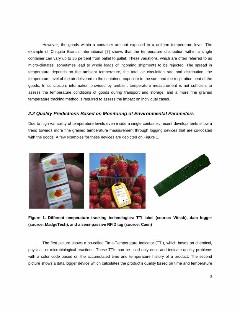
with the goods. A few examples for these devices are depicted on Figure 1.

Figure 1. Different temperature tracking technologies: TTI label (source: Vitsab), data logger

(source: MadgeTech), and a semi-passive RFID tag (source: Caen)

The first picture shows a so-called Time-Temperature Indicator (TTI), which bases on chemical,

physical, or microbiological reactions. These TTIs can be used only once and indicate quality problems

with a color code based on the accumulated time and temperature history of a product. The second

picture shows a data logger device which calculates the product’s quality based on time and temperature

4

and visualizes the result with an LED. In contrast to the TTI, it can be used multiple times, has a battery

life of 90 days and allows the temperature history to be read out through a serial interface. The last

picture shows a semi-passive RFID tag equipped with a temperature sensor. The sensor tag has a

battery life of five years and allows the temperature history to be read out through a radio frequency (RF)

interface. In comparison to the other two technologies, the sensor tag allows for uses with multiple

different products and for real-time data integration in supply chains. Due to the longer battery life, the

costs can be amortized over time and thus make supply chain monitoring of products economically

feasible. Recent advances aim for even smaller RFID tags with multiple integrated sensors for gas,

humidity, temperature, light, and vibration measurements.

2.3 Carbon Footprint

Depending on the product category and targeted consumer group, companies are used to optimize their

supply chain processes for cost, speed, quality, safety, and other key performance indicators. GHG

emissions only recently appeared on the list of important target figures. However, alongside the ongoing

debate on climate change, a growing number of companies start to collect the emission data that results

from their production and service provision.

GHG or carbon accounting methods may not only be applied to countries or organizations but

also to individual products. On a product level, life cycle assessments (LCA) help to determine what is

often referred to as the carbon footprint of goods. The carbon footprint ideally includes emissions related

to production, transportation, storage, use, recycling/disposal, and loss rates and may also capture other

climate gases such as methane that are accounted for after are multiplication with an impact factor and

expressed as CO2-equivalents.

Another measure that is important in the context of emission reductions are the CO2 abatement

costs. They express how much a stakeholder has to invest in order to lower the emission by a certain

amount. For some investments, the abatement cost can be negative. Energy-saving lamps, for example,

may not only reduce GHG emissions but also save money due to lower electricity bills that make up for

higher one-time costs. We will use the concept of abatement costs to evaluate the implications of the

sensor-based supply chain application.

5

3 Case Study

Our study is based on a research project with a major Swiss retailer. We use the example of strawberries

in Switzerland to investigate the value of sensor information for profit increase and carbon footprint

reduction in retail supply chains. The simulation parameters have been elicited in several discussions and

were validated with industry experts.

The Swiss consume approximately 16,500t of strawberries per year. As the domestic crop yield is

only able to satisfy a demand of 5,500t and due to seasonality of the product, the resulting gap of 66

percent needs to be filled by imports from neighbor and other countries. Suppliers and distribution routes

change frequently and therefore quality drops are likely to occur between the supplier to retailer link.

While strawberries are famous to consumers for their delicious taste, retailers perceive them as a difficult

product class with high loss rates. Sensors can be used to reduce these high loss rates by tracking the

fluctuations in environmental parameters on a case level. In this context, the order of which items are

depleted from stock or shelf, defined by the so-called issuing policy, is important to minimize the number

of perished items. Studies show that the use of a sensor based First-Expire-First-Out (FEFO) issuing

policy can increase a retailer’s profit tremendously [8, 9]. However, the use of sensors in a supply chain

introduces not only additional costs, but also additional emissions required for manufacturing,

transporting, and disposing sensors. While the impact on profit is often positive, the impact of sensor-

based management approaches on emission levels is yet to be explored.

With this background, we simulate the supply chain of a particular retailer, which wants to

evaluate sensor technologies with regard to its impact on profits and emission levels. In particular, we

investigate the carbon footprint of products, expressed as Global Warming Potential (GWP) in kg CO2

equivalents as defined in the CML 2001 method [10]. We compare a conventional scenario based on the

widely established First-In-First-Out (FIFO) issuing policy against a sensor based scenario with FEFO

issuing. In the sensor based scenario, Reusable Plastic Containers (RPC), which are used to transport

items throughout the supply chain, are equipped with temperature sensors. The FEFO issuing policy is

enabled through the knowledge of the temperature history, which allows calculating the remaining

keeping quality of products in a RPC.

3.1 Supply Chain Simulation Model

The basis for our analysis is a typical setting in the retail industry. A retailer sells a perishable product at

price to consumers and receives replenishments from a supplier. As Figure 2 illustrates, the supplier

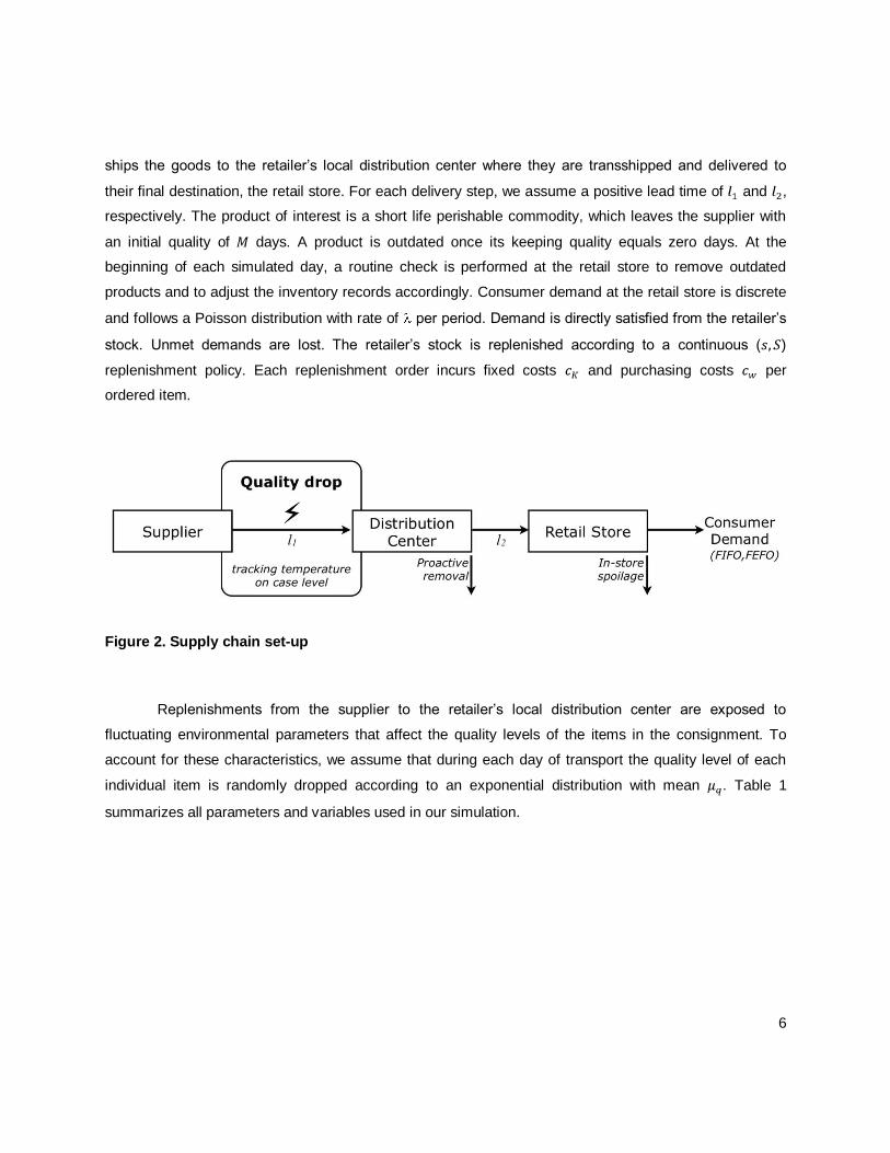
6

ships the goods to the retailer’s local distribution center where they are transshipped and delivered to

their final destination, the retail store. For each delivery step, we assume a positive lead time of and ,

respectively. The product of interest is a short life perishable commodity, which leaves the supplier with

an initial quality of days. A product is outdated once its keeping quality equals zero days. At the

beginning of each simulated day, a routine check is performed at the retail store to remove outdated

products and to adjust the inventory records accordingly. Consumer demand at the retail store is discrete

and follows a Poisson distribution with rate of per period. Demand is directly satisfied from the retailer’s

stock. Unmet demands are lost. The retailer’s stock is replenished according to a continuous ( )

replenishment policy. Each replenishment order incurs fixed costs and purchasing costs per

ordered item.

Figure 2. Supply chain set-up

Replenishments from the supplier to the retailer’s local distribution center are exposed to

fluctuating environmental parameters that affect the quality levels of the items in the consignment. To

account for these characteristics, we assume that during each day of transport the quality level of each

individual item is randomly dropped according to an exponential distribution with mean . Table 1

summarizes all parameters and variables used in our simulation.

7

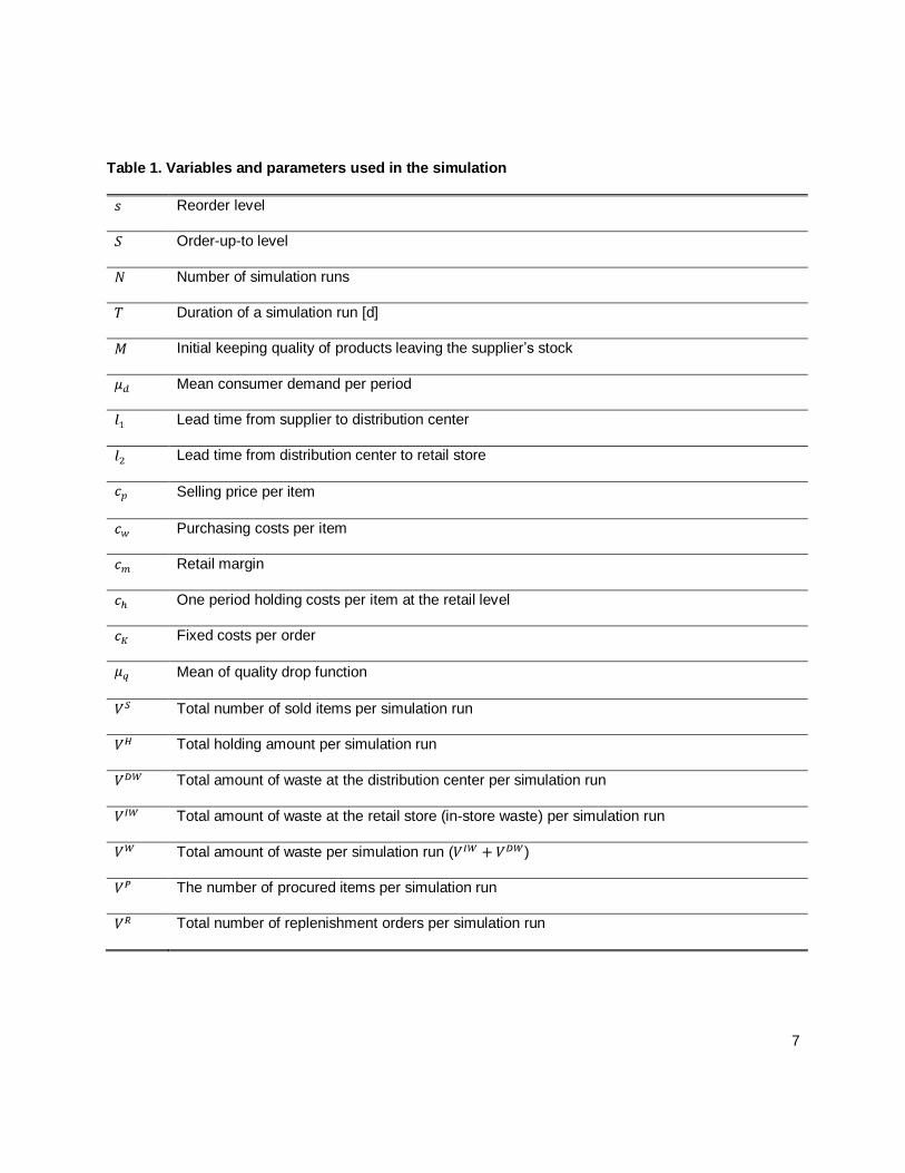
Table 1. Variables and parameters used in the simulation

Reorder level

Order-up-to level

Number of simulation runs

Duration of a simulation run [d]

Initial keeping quality of products leaving the supplier’s stock

Mean consumer demand per period

Lead time from supplier to distribution center

Lead time from distribution center to retail store

Selling price per item

Purchasing costs per item

Retail margin

One period holding costs per item at the retail level

Fixed costs per order

Mean of quality drop function

Total number of sold items per simulation run

Total holding amount per simulation run

Total amount of waste at the distribution center per simulation run

Total amount of waste at the retail store (in-store waste) per simulation run

Total amount of waste per simulation run ( )

The number of procured items per simulation run

Total number of replenishment orders per simulation run

8

For our experiments, we compare two different scenarios. In the first one, temperature data

about the products is not gathered and therefore employees must base their decisions on discernible

visual changes of the individual items. We refer to this scenario as the “classical approach”. In the second

scenario, sensors attached to transport cases (i.e. reusable plastic crates) record temperature deviations

and therefore allow decisions based on effective quality levels of products to be made. Employees can

use this information to make informed decisions beyond their visual capabilities. Due to sensor

information, employees are able to presort items according to a FEFO issuing policy already at the

distribution level. In practice, no additional personnel are required because presorting could simply be

achieved during the picking operation by means of an additional sort parameter on the picking list. In

addition, items with an overly low quality are directly discarded if their keeping quality is less or equal the

transport lead time . We refer to this scenario as the “sensor-enhanced approach”.

3.2 Objective Functions

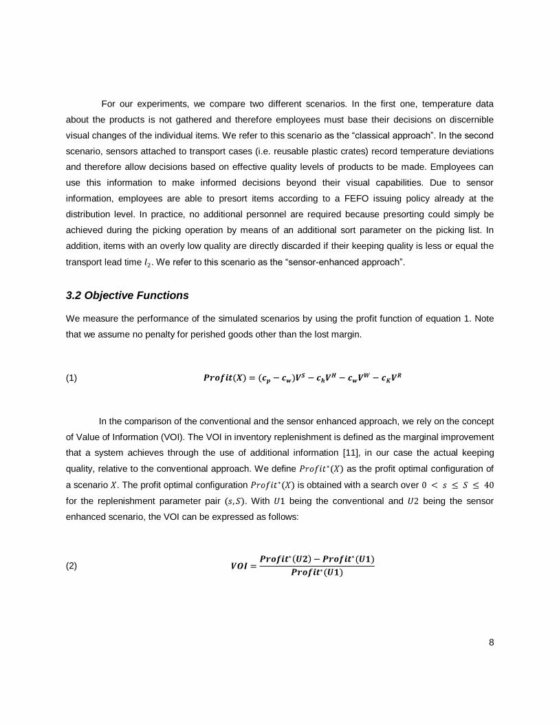
We measure the performance of the simulated scenarios by using the profit function of equation 1. Note

that we assume no penalty for perished goods other than the lost margin.

(1)

In the comparison of the conventional and the sensor enhanced approach, we rely on the concept

of Value of Information (VOI). The VOI in inventory replenishment is defined as the marginal improvement

that a system achieves through the use of additional information [11], in our case the actual keeping

quality, relative to the conventional approach. We define as the profit optimal configuration of

a scenario . The profit optimal configuration is obtained with a search over

for the replenishment parameter pair . With being the conventional and being the sensor

enhanced scenario, the VOI can be expressed as follows:

(2)

9

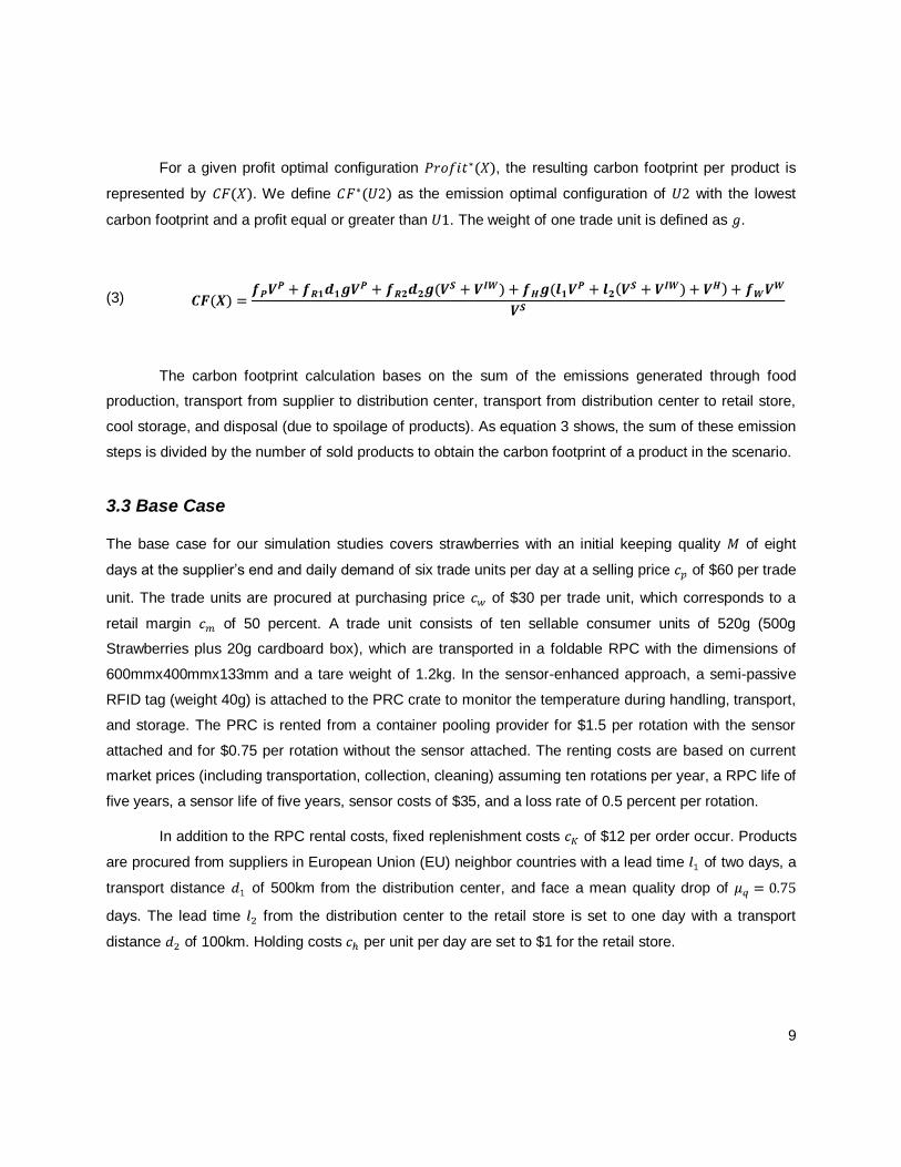
For a given profit optimal configuration , the resulting carbon footprint per product is

represented by . We define as the emission optimal configuration of with the lowest

carbon footprint and a profit equal or greater than . The weight of one trade unit is defined as .

(3)

The carbon footprint calculation bases on the sum of the emissions generated through food

production, transport from supplier to distribution center, transport from distribution center to retail store,

cool storage, and disposal (due to spoilage of products). As equation 3 shows, the sum of these emission

steps is divided by the number of sold products to obtain the carbon footprint of a product in the scenario.

3.3 Base Case

The base case for our simulation studies covers strawberries with an initial keeping quality of eight

days at the supplier’s end and daily demand of six trade units per day at a selling price of $60 per trade

unit. The trade units are procured at purchasing price of $30 per trade unit, which corresponds to a

retail margin of 50 percent. A trade unit consists of ten sellable consumer units of 520g (500g

Strawberries plus 20g cardboard box), which are transported in a foldable RPC with the dimensions of

600mmx400mmx133mm and a tare weight of 1.2kg. In the sensor-enhanced approach, a semi-passive

RFID tag (weight 40g) is attached to the PRC crate to monitor the temperature during handling, transport,

and storage. The PRC is rented from a container pooling provider for $1.5 per rotation with the sensor

attached and for $0.75 per rotation without the sensor attached. The renting costs are based on current

market prices (including transportation, collection, cleaning) assuming ten rotations per year, a RPC life of

five years, a sensor life of five years, sensor costs of $35, and a loss rate of 0.5 percent per rotation.

In addition to the RPC rental costs, fixed replenishment costs of $12 per order occur. Products

are procured from suppliers in European Union (EU) neighbor countries with a lead time of two days, a

transport distance of 500km from the distribution center, and face a mean quality drop of

days. The lead time from the distribution center to the retail store is set to one day with a transport

distance of 100km. Holding costs per unit per day are set to $1 for the retail store.

10

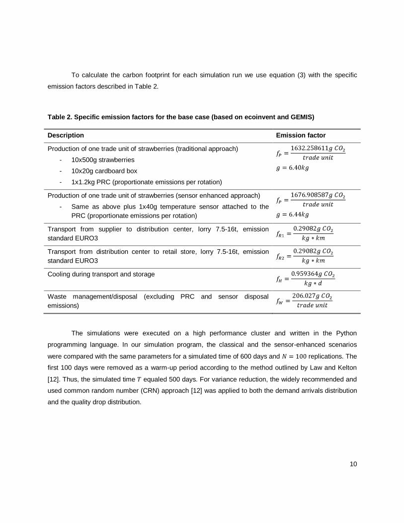
To calculate the carbon footprint for each simulation run we use equation (3) with the specific

emission factors described in Table 2.

Table 2. Specific emission factors for the base case (based on ecoinvent and GEMIS)

Description Emission factor

Production of one trade unit of strawberries (traditional approach)

- 10x500g strawberries

- 10x20g cardboard box

- 1x1.2kg PRC (proportionate emissions per rotation)

Production of one trade unit of strawberries (sensor enhanced approach)

- Same as above plus 1x40g temperature sensor attached to the

PRC (proportionate emissions per rotation)

Transport from supplier to distribution center, lorry 7.5-16t, emission

standard EURO3

Transport from distribution center to retail store, lorry 7.5-16t, emission

standard EURO3

Cooling during transport and storage

Waste management/disposal (excluding PRC and sensor disposal

emissions)

The simulations were executed on a high performance cluster and written in the Python

programming language. In our simulation program, the classical and the sensor-enhanced scenarios

were compared with the same parameters for a simulated time of 600 days and replications. The

first 100 days were removed as a warm-up period according to the method outlined by Law and Kelton

[12]. Thus, the simulated time equaled 500 days. For variance reduction, the widely recommended and

used common random number (CRN) approach [12] was applied to both the demand arrivals distribution

and the quality drop distribution.

11

3.4 Base Case Results

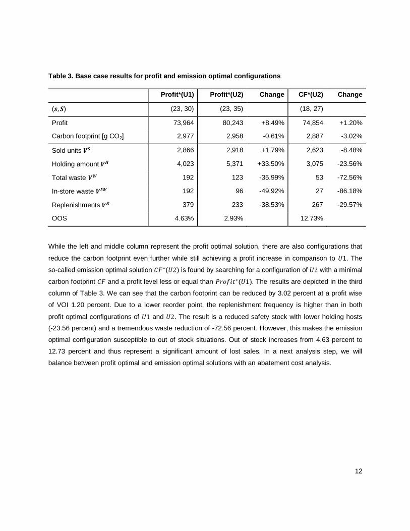
Table 3 shows the results and averaged performance metrics for the simulation runs with respect to profit

optimal and emission optimal configurations. The left and middle column represent the profit optimal

configurations for , the classical approach and , the sensor enhanced approach. The profit increase

of over , namely the VOI, amounts to 8.49 percent. The 99 percent confidence interval for the mean

profit increase is 0.2 percent. As Table 3 shows, the profit increase is based mainly on the decreased

number of unsellable goods (-35.99 percent) and the decreased number of out-of-stocks (-36.83 percent).

This confirms that the sensor-based approach is more resource efficient than the traditional approach.

Since fewer products are thrown away, the holding costs rise as the retail shelf space is better utilized

(+33.50 percent). By sensor enhanced sorting due to the FEFO policy, the amount of in-store waste

decreases by 49.92 percent. Interestingly, this has also positive impact on the emission levels. Due to

sensor information, the total emissions (which are driven by the number of sold units) are be reduced by

0.66 percent. However, the real impact on emission levels is even greater. The carbon footprint per sold

trade unit is reduced by 0.61 percent as resource efficiency increases. In conclusion, while having

optimized for profit, the sensor enhanced approach was also superior to the classical approach with

respect to the carbon footprint. In the base case, the costs and emissions associated with the introduction

of the sensor technology into the supply chain are therefore negligible in comparison to the benefits

achieved.

12

Table 3. Base case results for profit and emission optimal configurations

Profit*(U1) Profit*(U2) Change CF*(U2) Change

( ) (23, 30) (23, 35) (18, 27)

Profit 73,964 80,243 +8.49% 74,854 +1.20%

Carbon footprint [g CO2] 2,977 2,958 -0.61% 2,887 -3.02%

Sold units 2,866 2,918 +1.79% 2,623 -8.48%

Holding amount 4,023 5,371 +33.50% 3,075 -23.56%

Total waste 192 123 -35.99% 53 -72.56%

In-store waste 192 96 -49.92% 27 -86.18%

Replenishments 379 233 -38.53% 267 -29.57%

OOS 4.63% 2.93% 12.73%

While the left and middle column represent the profit optimal solution, there are also configurations that

reduce the carbon footprint even further while still achieving a profit increase in comparison to . The

so-called emission optimal solution is found by searching for a configuration of with a minimal

carbon footprint and a profit level less or equal than . The results are depicted in the third

column of Table 3. We can see that the carbon footprint can be reduced by 3.02 percent at a profit wise

of VOI 1.20 percent. Due to a lower reorder point, the replenishment frequency is higher than in both

profit optimal configurations of and . The result is a reduced safety stock with lower holding hosts

(-23.56 percent) and a tremendous waste reduction of -72.56 percent. However, this makes the emission

optimal configuration susceptible to out of stock situations. Out of stock increases from 4.63 percent to

12.73 percent and thus represent a significant amount of lost sales. In a next analysis step, we will

balance between profit optimal and emission optimal solutions with an abatement cost analysis.

13

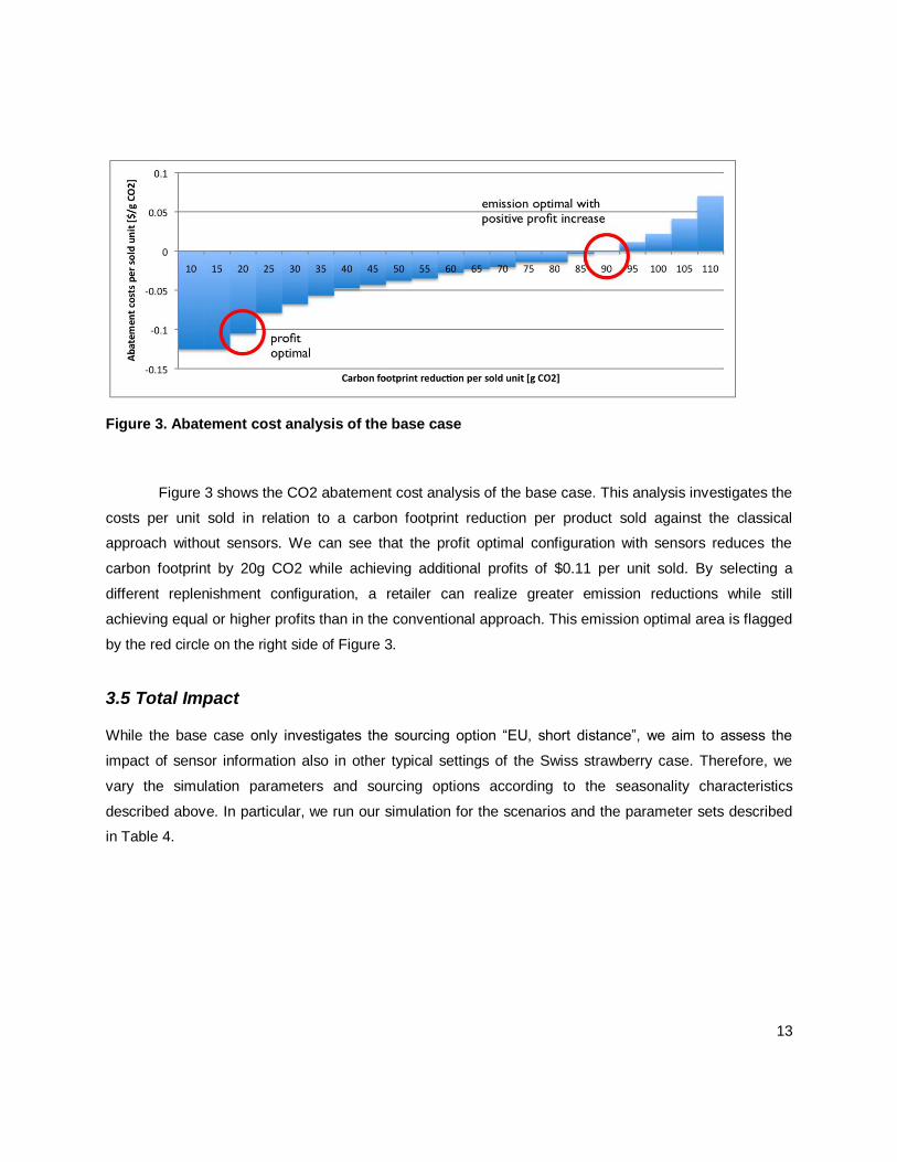
Figure 3. Abatement cost analysis of the base case

Figure 3 shows the CO2 abatement cost analysis of the base case. This analysis investigates the

costs per unit sold in relation to a carbon footprint reduction per product sold against the classical

approach without sensors. We can see that the profit optimal configuration with sensors reduces the

carbon footprint by 20g CO2 while achieving additional profits of $0.11 per unit sold. By selecting a

different replenishment configuration, a retailer can realize greater emission reductions while still

achieving equal or higher profits than in the conventional approach. This emission optimal area is flagged

by the red circle on the right side of Figure 3.

3.5 Total Impact

While the base case only investigates the sourcing option “EU, short distance”, we aim to assess the

impact of sensor information also in other typical settings of the Swiss strawberry case. Therefore, we

vary the simulation parameters and sourcing options according to the seasonality characteristics

described above. In particular, we run our simulation for the scenarios and the parameter sets described

in Table 4.

14

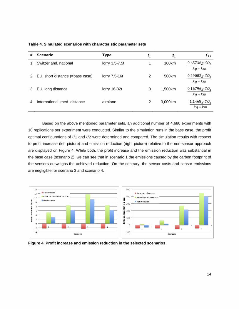
Table 4. Simulated scenarios with characteristic parameter sets

# Scenario Type

1 Switzerland, national lorry 3.5-7.5t 1 100km

2 EU, short distance (=base case) lorry 7.5-16t 2 500km

3 EU, long distance lorry 16-32t 3 1,500km

4 International, med. distance airplane 2 3,000km

Based on the above mentioned parameter sets, an additional number of 4,680 experiments with

10 replications per experiment were conducted. Similar to the simulation runs in the base case, the profit

optimal configurations of and were determined and compared. The simulation results with respect

to profit increase (left picture) and emission reduction (right picture) relative to the non-sensor approach

are displayed on Figure 4. While both, the profit increase and the emission reduction was substantial in

the base case (scenario 2), we can see that in scenario 1 the emissions caused by the carbon footprint of

the sensors outweighs the achieved reduction. On the contrary, the sensor costs and sensor emissions

are negligible for scenario 3 and scenario 4.

Figure 4. Profit increase and emission reduction in the selected scenarios

15

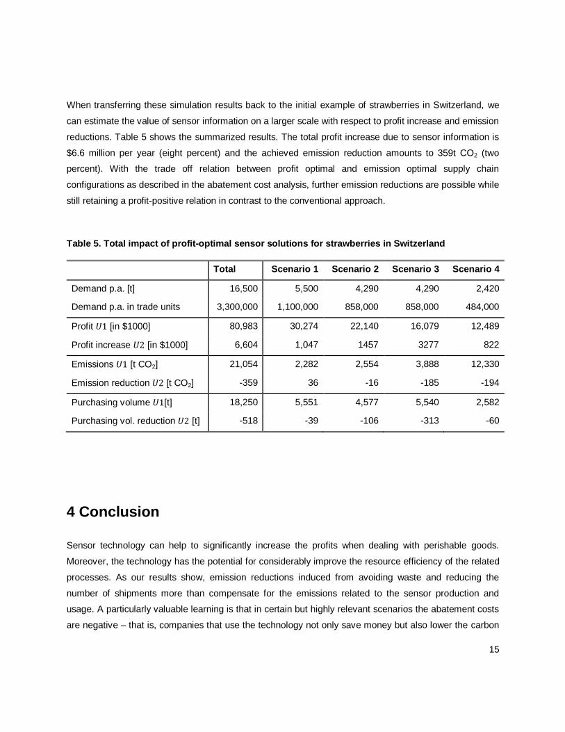
When transferring these simulation results back to the initial example of strawberries in Switzerland, we

can estimate the value of sensor information on a larger scale with respect to profit increase and emission

reductions. Table 5 shows the summarized results. The total profit increase due to sensor information is

$6.6 million per year (eight percent) and the achieved emission reduction amounts to 359t CO2 (two

percent). With the trade off relation between profit optimal and emission optimal supply chain

configurations as described in the abatement cost analysis, further emission reductions are possible while

still retaining a profit-positive relation in contrast to the conventional approach.

Table 5. Total impact of profit-optimal sensor solutions for strawberries in Switzerland

Total Scenario 1 Scenario 2 Scenario 3 Scenario 4

Demand p.a. [t] 16,500 5,500 4,290 4,290 2,420

Demand p.a. in trade units 3,300,000 1,100,000 858,000 858,000 484,000

Profit [in $1000] 80,983 30,274 22,140 16,079 12,489

Profit increase [in $1000] 6,604 1,047 1457 3277 822

Emissions [t CO2] 21,054 2,282 2,554 3,888 12,330

Emission reduction [t CO2] -359 36 -16 -185 -194

Purchasing volume [t] 18,250 5,551 4,577 5,540 2,582

Purchasing vol. reduction [t] -518 -39 -106 -313 -60

4 Conclusion

Sensor technology can help to significantly increase the profits when dealing with perishable goods.

Moreover, the technology has the potential for considerably improve the resource efficiency of the related

processes. As our results show, emission reductions induced from avoiding waste and reducing the

number of shipments more than compensate for the emissions related to the sensor production and

usage. A particularly valuable learning is that in certain but highly relevant scenarios the abatement costs

are negative – that is, companies that use the technology not only save money but also lower the carbon

16

footprint of their products. Other beneficial environmental effects (such as less land use) and monetary

effects (such as better image of the company and price premium for suitably handled products) are not

even included in this consideration. Based on these results, we can recommend with confidence

exploring and putting into practice similar supply chain applications.

Future research should include the development of novel issuing policies that make use of the

enhanced insights into the history of products, the consideration of other environmental parameters such

as vibration and shock, the design of low-cost monitoring devices, and the development of solutions

where products actively control their environmental conditions.

5 References

1. First Research, Grocery Stores and Supermarkets Industry Profile, NAICS Code: 44511, First Research, 2005.

2. A. Goldman, et al., “Barriers to the advancement of modern food retail formats: theory and measurement,”

Journal of Retailing, vol. 78, no. 4, 2002, pp. 281-295.

3. Tsiros and Heilman, “The Effect of Expiration Dates and Perceived Risk on Purchasing Behavior in Grocery

Store Perishable Categories,” Journal of Marketing, vol. 69, no. 2, 2005, pp. 114-129.

4. R.E. Krider and C.B. Weinberg, “Product perishability and multistore grocery shopping,” Journal of Retailing and

Consumer Services, vol. 7, no. 1, 2000, pp. 1-18.

5. DEFRA, Report of the Food Industry Sustainability Strategy Champions' Group on Food Transport, Department

for Environment, Food and Rural Affairs, 2007.

6. European Commission, Environmental Impact of Products (EIPRO): Analysis of the life cycle environmental

impacts related to the final consumption of the EU-25, Technical Report EUR 22284 EN, European Comission,

2006.

7. M.C. O'Connor, “Cold-Chain Project Reveals Temperature Inconsistencies,” RFID Journal, 2006;

http://www.rfidjournal.com/article/articleview/2860/2/1/.

8. M.C. Giannakourou and P.S. Taoukis, “Application of a TTI-based Distribution Management System for Quality

Optimization of Frozen Vegetables at the Consumer End,” Journal of Food Science, vol. 68, no. 1, 2003, pp.

201-209; DOI doi:10.1111/j.1365-2621.2003.tb14140.x.

9. A. Dada and F. Thiesse, “Sensor Applications in the Supply Chain: The Example of Quality-Based Issuing of

Perishables,” The Internet of Things, 2008, pp. 140-154.

10. J.B. Guinée, Handbook on Life Cycle Assessment. Operational Guide to ISO Standards., Kluwer Academic

Publishers, 2002.

17

11. M.E. Ketzenberg, et al., “A framework for the value of information in inventory replenishment,” European Journal

of Operational Research, vol. 182, no. 3, 2007, pp. 1230-1250.

12. A.M. Law and D.M. Kelton, Simulation Modeling and Analysis, McGraw-Hill Higher Education, 2001.