....

.. ;~

•

-.:

USING RECURSIVE RESIDUALS, CALCULATED ON ADAPTIVELY-ORDERED

OBSERVATIONS, TO IDENTIFY OUTLIERS IN LINEAR REGRESSION

Farid Kianifard and William H. Swallow

Institute of Statistics Mimeo Series No. 19051{

September 1987

Department of St~tistics library

USING RECURSIVE RESIDUALS, CALCULATED ON ADAPTIVELy-oRDERBD

OBSERVATIONS, TO IDENTIFY OUTLIBRS IN LINEAR REGRBSSION

Farid Kianifard and William H. Swallow

Department of StatisticsNorth Carolina State University

Raleigh, NC 27695-8203

SUMMARY

A new procedure for identifying outliers or influential

observations is proposed. The procedure uses recursive residuals,

calculated on observations which have been ordered according to

their studentized residuals, values of Cook's D, or another regression

diagnostic of the user's choice. These recursive residuals,

appropriately standardized, have approximate Student's t

distributions. Thus, convenient critical values are available for

deciding which observations merit scrutiny and, perhaps, special

treatment. The power of the test procedure to identify one or more

outliers is investigated through simulation. Power is generally high,

but depends on the number and configuration of the outliers, that is,

their placement with respect to the main body of the data. The use

of adaptive ordering increases power and helps to combat the

masking of one outlier by another when multiple ouiliers are present.

Key Words: Cook's D; Influential observations; Regression diagnostics;

Studentized residual

-

L Introduction

Data from many fields are commonly analyzed using linear

regression. These data sets often contain outliers or influential

observations, and it is important that such observations be identified

in the course of a thorough statistical analysis. In some cases,

observations which fall outside the pattern seen in the bulk of the

data, and which are thus known as outliers, are important and of

interest in their own right. Indeed, they may be the most

interesting and important observations in the entire data set, and

their identification a matter of high priority. Identification of such

an outlier may direct future research effort to collecting additional

data in the region (treatment combination) where the interesting

outlier was observed.

Furthermore, it is always important to identify aberrant

observations, either valid outliers or erroneous data points, with an

eye to removing them from the data set or at least down-weighting

them in the analysis of the rest of the data. Clearly, erroneous data

should be corrected, if possible, or deleted. But even valid outliers

often should be set aside lest they have undue impact or influence

on the analysis, seriously distorting conclusions about relationships

between variables in the main body of the data. Such data points

are often called influential observations. Of course, removing

observations from data sets should not be undertaken lightly;

objective methods are required for identifying candidates for deletion

or other special treatment.

1

-

The study of outliers and influential observations in linear models

has attracted considerable interest in the past decade. A number of

books have been published devoted largely or exclusively to this

subject: Belsley, Kuh, and Welsch (1980), Hawkins (1980), Cook and

Weisberg (1982), Barnett and Lewis (1984), Atkinson (1985), Rousseeuw

and Leroy (1987), and Chatterjee and Hadi (1988). A recent review

article by Chatterjee and Hadi (1986) summarizes many of the

well-known outlier-identification statistics and their interrelationships.

We consider here the usual linear regression model:

-

Y = XR + e ,,.", ,.",~ ,..., (1.1)

where ! = (y " ...,yn)' is an n x 1 vector of values of the response

variable, ~ = (~""',~p)' is a p x 1 vector of unknown parameters,

X =(x;,...,x~)' is an n x p matrix of explanatory variables with,.. ,.. ,..

rank(X) = p, and e = (eu... ,8 n)' is an n x 1 vector of independent,.. ,..

normal random variables with mean 0 and (unknown) variance er2 •

For ~ =qr~)-l:r!, the ordinary least squares (OLS) estimator of ~,

the vector of OLS residuals is given by

..~ =! - !t!.

= (! - !D!

where H =(hi j)

er 2 is then

=X(X'X)-lX'.Ill' ,.,., ,.,

The residual mean square estimate of

2

The OLS residuals e t are correlated and their variances differ as

is evident from their variance-covariance matrix:

2Yar(e) = a (I - H) •... ... ... (1.2)

As equation (1.2) implies, the distribution of the OLS residuals even

depends, through ~, on the particular design matrix! being

considered.

A scaled version of the e t can be defined as -%e . =e./s(l - h .. ) ,

S1 1 11i = l, •.• ,n • (1.3)

The e.t are usually called the studentized residuals (STUDENT in

SAS), the name we will use. Other authors have called them the

standardized residuals or internally studentized residuals. Another·

scaled version of the et, advocated by Belsley et ale (1980) and

others, is often called the jackknifed or externally studentized

residual (RSTUDENT in SAS), and is defined as

%t. = e./s(.)(l - h .. ) ,1 1 1 11

i = l, ••• ,n , (1.4)

where S2 ( t) is the residual mean square estimate of a 2 obtained with

the i th observation omitted. Atkinson (1981) called tt the

"cross-validatory" residual and, noting that

tt = e.d(n-p-l)/(n-p-e~t)}, pointed out that the tt are a monotone

transformation of the e. t. While the above scaled versions of the

residuals e t have approximately unit variance, they are still

correlated.

A common practice is to plot the least squares residuals or e.t

or tt against variables such as t t or one or more of the explanatory

3

variables, or in serial order, to detect outliers. These plots sutfer

from the fact that the impact of an outlier is not confined to inflating

only its own e1' e.1 or t 1; it may inflate or deflate the e1' e s 1' or t 1

of other observations too, perhaps making itself more or less

conspicuous in the process. In simple linear regression, for example,

an outlier that is influential in determining the slope of the fitted

line draws the line toward itself, tending to inflate residuals

associated with other observations, while giving itself a smaller

residual than one might expect. Outliers also inflate the s( 1) or s

used to scale the t 1 or e s 1' respectively. When a single outlier is

present, s( 1) will be unaffected for the outlier, but inflated for all

other observations; the t 1 for nonoutliers will then shrink, leaving

the outlier more exposed. When multiple outliers are present, concern

about masking (outliers hiding each other) and swamping (making

nonoutliers appear to be outliers) is much greater. Multiple outliers

can reinforce or cancel each others' influence, presenting the data

analyst with a difficult and potentially confusing outlier-identification

problem. Concerns about masking and swamping are. by no means

specific to simple graphical procedures; attempts to use the e1' e.1'

or t 1 nongraphically are affected too.

Detecting outliers which are influential is of particular interest.

Of course, different observations may be influential in different

calculations; the estimation of the parameter vector fJ is generally aN

calculation of prime interest. Cook's (1977) D is a well-known measure

of influence of the i1:h observation on e. It is defined as

4

-

(1.5)

where ~ ( ,) is the ordinary least squares estimate of ~ obtained after

deleting the ii:h observation. Chatterjee and Hadi (1986) give some

alternative measures of influence, preferred by some data analysts,

but closely akin to Cook's D..-

Measures of the influence of the ii:h observation on ethrough

Var(~) can be based on the change in the volume of confidence

ellipsoids when the i'th observation is removed. One such measure,

introduced by Belsley et al. (1980), is

-

(1.6)

COVRATIO t is a ratio of the estimated generalized variances (see, e.g.,

Theil, 1971, p. 124) of the regression coefficients with and without the

ii:h observation deleted from the data, and, therefore, it can be

interpreted as a measure of the effect of the i th observation on the

efficiency of estimating fJ. A value of COVRATIO, greater than one...indicates that deleting the ii:h observation impairs efficiency, whereas

a value less than one indicates increased efficiency of estimation.

Atkinson (1981) has suggested using half-normal plots of t t or of

a modified version of Cook's D with simulated envelopes. This

approach seems quite effective in identifying outliers and influential

observations, but poses a substantial computational burden.

Obtaining the envelopes (bounds) requires simulating and analyzing

some 20 or more samples, a serious drawback for application to large

5

samples or routine screening. For a more complete discussion of this

approach, see Atkinson (1985).

Packaged programs [e.g., BMDP(09R), Minitab, SAS(PROC REG),

SPSS(New Regression)] nowadays provide a selection of the above

and/or other regression diagnostics and measures of influence.

Multiple-case diagnostics to identify groups (subsets) of outlying

and/or influential observations also exist, including

algebraically-straightforward generalizations of single-case diagnostics

like Cook's D of (L5). These too are likely to require a formidable

computational effort for even moderate-sized data sets and have not

sparked much interest among practitioners; they have not been

implemented in packaged programs. In practice, data analysts

generally rely on single-case diagnostics, despite their vulnerability

to masking and swamping when multiple outliers are present.

In this article, we develop a procedure based on recursive

residuals (Brown, Durbin, and Evans, 1975) for identifying (one or

more) outliers or influential observations in a linear regression

analysis. The procedure is described in Section 3, and its properties

investigated in a simulation study described in Section 4. An example

of application to a well-known data set is given in Section 5.

Although by no means do we advocate automatic deletion of

observations by a packaged program using this or any other

diagnostic or procedure, this procedure is suitable for routine

screening to identify points that deserve scrutiny and perhaps

special treatment.

6

-

2. Recursive Residuals

Consider the regression model (1.1) with independent

identically-distributed (iid) normal errors~. Let !J-l denote the

(j-l) x p matrix consisting of the first j-l rows (observations) of X.N

Provided (j-l) L p and assuming (!j-l!J-l) to be nonsingular, ecan

be estimated by

(2.1)

-where !J-l denotes the subvector consisting of the first j-l elements

of 'Y. Using eJ-u one can "forecast" YJ to be ~jeJ-1" The forecast

error is the difference (y J - !j~J-t>, and the variance of this

forecast error is cr2[l + ~j(!J-l!J-d-l~J]. The recursive residuals

are defined as

j =p+1, ••• ,D • (2.2)

Brown et al. (1975, Lemma 1) show that, under the model, and

assuming the inverses (!j-l !J-l )-1 exist for all j-l L p, Wp+l,...,Wn

are independent N(O,cr 2 ). This will be true for recursive residuals

calculated on randomly-ordered observations, or on observations

which have been ordered by any variable which is statistically

independent of the wJ [e.g., values of an x variable or of

!J = !~J-l for any of the ~J-l of (2.1)]; the values of the recursive

residuals will depend on the order in which they are calculated, but

their distribution will not. Recursive residuals cannot be calculated

for the first p observations. Hedayat and Robson (1970) defined the

7

recursive residuals in an alternative form and called them "stepwise

residuals"•

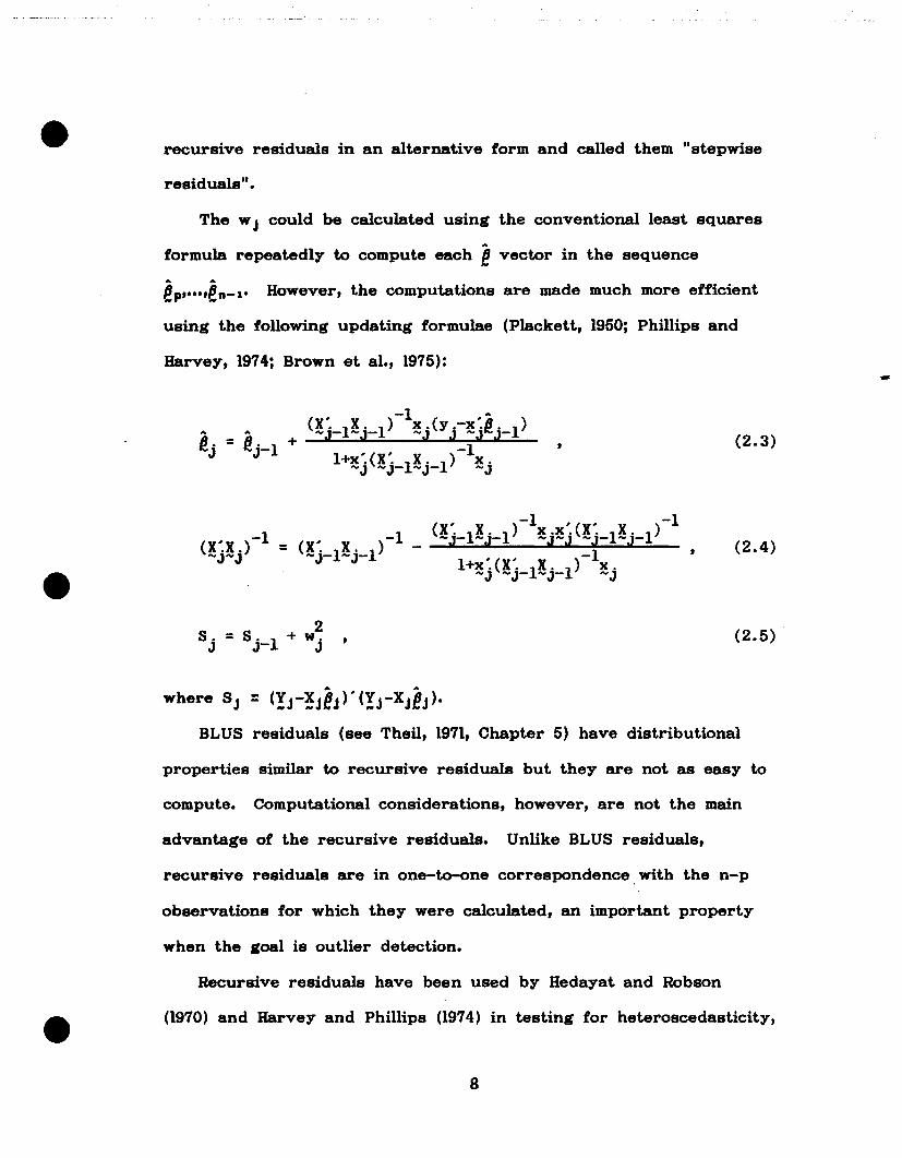
The w j could be calculated using the conventional least squares

formula repeatedly to compute each evector in the sequence

~p,.",~n-l. However, the computations are made much more efficient

using the following updating formulae (Plackett, 1950; Phillips and

Harvey, 1974; Brown et al., 1975): -(2.3)

2S.=S·l+ w .

J J- J

(2.4)

(2.5) .

where 5 J = (!j-!jej)'(!j-Xjej).

BLU5 residuals (see Theil, 1971, Chapter 5) have distributional

properties similar to recursive residuals but they are not as easy to

compute. Computational considerations, however, are not the main

advantage of the recursive residuals. Unlike BLU5 residuals,

recursive residuals are in one-to-one correspondence. with the n-p

observations for which they were calculated, an important property

when the goal is outlier detection.

Recursive residuals have been used by Hedayat and Robson

(1970) and Harvey and Phillips (1974) in testing for heteroscedasticity,

8

by Phillips and Harvey (1974) in constructing an exact test for first

order autocorrelation using the von Neumann ratio, by Brown et ale

(1975) in testing for structural change over time, and by Harvey and

Collier (1977) in testing for possible model misspecifications. Galpin

and Hawkins (1984) proposed the use of recursive residuals in

graphical procedures to check the model assumptions. Du Toit,

Steyn, and Stumpf (1986) provided a program for calculating

recursive residuals and using them in normal probability and

cumulative sum plotting; their program uses PROC MATRIX in SASe

3. The Test Procedure

To motivate our approach, we quote some remarks about recursive

residuals from Barnett and Lewis (1984, p. 294):

"These would seem to have potential for the study of

outliers, although no progress on this front is evident.

There is a major difficulty in that the labelling of the

observations is usually done at random, or in relation to

some concomitant variable, rather than •adaptively' in

response to the observed sample values (which might be a

desirable prospect from the outlier standpoint)."

Accordingly, we propose the following strategy for labelling or

ordering the observations, and calculating recursive residuals and

test statistics:

1) Fit the regression model to the data.

9

-

2) Compute values of an appropriate regression diagnostic

(e.g., the studentized residual or Cook's D) for each of the

n observations.

3) Order the observations according to the chosen diagnostic

measure.

4) Use the first p observations in the ordered data set to form

the "basis" for computing recursive residuals.

5) Compute recursive residuals, w j' for the remaining (n-p)

ordered observations.

6) Calculate the statistics w j/S( t), j =p+l,... ,n, comparing

the computed values against values of Student's t with

n-p-l df.

Under (1.1) with normality, the (unordered) recursive residuals w j

are iid N(0,0'2) random variables. Hence, if we were to estimate 0'2 by

a.J, an estimate of 0'2 which was independent of w j' then w j/a. j would

have an exact t distribution with the degrees of freedom (df) of a.J.

To test the null hypothesis that the jt:h observation is not an outlier,

we could then compare each w j fa. j to percentiles of the appropriate t

distribution and reject the null hypothesis whenever Iw j fa. j I

exceeded the critical value of t. The same would be true when

recursive residuals w j were calculated on observations which had

been ordered by any variable which was statistically independent of

those w j • Such ordering variables include the hi i' the diagonal

entries of the hat matrix ~ =~(~'~)-I~', which are sometimes used

as a measure of leverage. However, in general, when the

10

-

observations are adaptively ordered, the ordering variable will not be

independent of the recursive residuals, and the exact N(O,O' 2 )

property of the recursive residuals will be voided. Furthermore,

there are compelling reasons to use estimates of 0'2 that may not be

independent of the Wj (see Section 4); the estimate of 0'2 we adopt

and advocate is s 2 ( i) used for t i of (1.4). The test statistics W l s ( i )

have approximate t distributions under the null hypotheses.

When an appropriate diagnostic measure is used to order the

observations, outliers and/or influential observations can be expected

to appear late in the sequence of recursive residuals. The W j for

data points which precede them in the ordered set then, by

construction, will be unaffected by these outliers, reducing the

potential for masking and swamping. The adaptive ordering also

makes it highly unlikely that outliers will appear among the first p

ordered observations for which no recursive residuals are calculated

and no tests are possible; that is, the ordering Yields a "clean" basis

set for calculating recursive residuals.

We consider here three diagnostic measures according to which

the observations could be ordered,c arranging them in ascending

order of Ie 8 i I or D i or in descending order of COVRATIO i. These

measures represent different classes of regression diagnostics.

The studentized residual, e. i' of (1.3), was chosen over t i of (1.4)

because it is better known and more widely available through

packaged statistical programs. Because t i is a monotone function of

es 1' both give the same ordering. Similarly, Cook's D was chosen

11

because it is more widely known and available than other

closely-related measures: DFFITS and the Modified Cook's D

(Chatterjee and Hadi, 1986). The COVRATIO is less widely available

through standard packages, but represents a different class of

diagnostics. We did not use the htt, because they identify only

outliers with respect the x range, but take no account of

observations outlying in the response variable y.

4. Properties of the Test Procedure

We now present simulation results, first to justify our choice of

S( t) as the most suitable estimate of a, and then to evaluate the

performance of the test procedure suggested in Section 3 (referred

to hereafter as the "recursive method"). We used a simple linear

regression model Yt =flo + fllxt + B t with n =25 in all simulations

discussed here. The residuals are unaffected by the particular

values of flo and fll used; we set flo = 0, fll = 1. The x's were

generated as uniform (0,1) variables multiplied by 15. The error

terms B t were generated as N(O,I) random variables. Necessary

modifications were made to introduce outliers as described below. All

results are based on 1000 simulated samples of n = 25 each, with the

x's regenerated after every 100 samples. The same 10 sets of x's

were used in all simulations. The nominal level of the test was

ex = .05 throughout.

Table 1 shows the ex-levels of the test observed in our simulations

using different estimates of a with and without ordering by the

12

-

studentized residual. The estimates sand s ( i) are as defined in

Section 1 and

j-1 %80_1 ={I W~/(j-3)} ,

J i=3 1j=4, ... ,25. (4.1)

...The estimates Sj-l are paired with the ej-l of (2.1) used to obtain

the recursive residuals in (2.2); for a fixed value of j-l, SJ-l is

nothing more than the usual error mean square estimate of 0'2

obtained by fitting a line to the first j-l observations only. We

calculate Sj-l in (4.1) using the relation that, for a given fitted line,

the sum of squares of ordinary residuals equals the sum of squares

of recursive residuals (the first p being identically zero). The

column headings in Table 1 correspond to the cases where the

observations were arranged according' to increasing values of Ie s i I

and when there was no ordering. For the unordered case, Sj-l is

clearly independent of Wj' and Wj/Sj_l will have an exact t

distribution.

Because recursive residuals, w j' are only calculated for j =

3,... ,25, only 23 are available for testing in each unordered sample.

When Sj-l is used, only 22 can be tested. When the sample is

ordered, we assume that outliers and influential observations will

appear late in the sequence and be tested, i.e., we assume that all 25

observations in each sample are effectively tested. The divisors used

in calculating the entries in Tables 1-3 were adjusted accordingly

(see footnotes to Tables 1, 2). The fact that an outlier could be

untested in the unordered case itself argues for preordering if

13

...

recursive residuals are to be used as the basis for an outlier

detection statistic.

Table I confirms that, for the unordered sample, using SJ-l yields

test statistics having exact t distributions. That notwithstanding, for

our purposes, Sj-l is unworkable. First, for unordered samples, an

outlier would be equally likely to appear anywhere in the sequence;

one could not test the first p+l observations at all, and other

observations which appeared early in the unordered sequence would

be tested with few degrees of freedom. Second, for the ordered

sample, the variance is underestimated badly for many of the test

statistics wJ/sJ-u leading to far too many rejections (Table 1).

----Insert Table I Here --

The variance estimates s 2 and s 2 ( 1) can be used with good

results, although we prefer s 2 ( 1). For either one, the size of the

test is essentially the same with and without ordering. When S2 is

used, the test is somewhat conservative. When S2 (1) is used, the

observed size of the test (.048) is seen to be very close to the

nominal ex = .05. When S2 ( t) was used and the observations ordered

by Cook's D or by the COVRATIO, the observed size was also .048

(results not shown). S2( t) has the further advantage that it is more

robust; if an observation is indeed an outlier, that will inflate the

numerator, but not the denominator, ~f wJ / S( t ). The results which

follow all use S( t ) •

14

Table 2 summarizes the performance of the recursive method

according to whether the observations are ordered by a diagnostic

measure or not. When the sample was to be "not ordered", a single

outlier was created as follows: A random observation number was

selected from numbers 3-25. This ensured that the outlier would be

tested, not be part of the basis set. An amount 6 was then added to

the generated x value for that observation in place of a simulated

error term; recall flo =0, fll =1, and a =1, SO using 6 =3, for

example, is equivalent to placing the outlier 3 standard deviations

above the (true) line. In cases where the data would be ordered by

a diagnostic measure, the outlier was created by adding 6 to the 25i:h

generated x value (without loss of generality as the observations are

reordered) in place of a simulated error. Obvious generalizations

were used in creating as many as 3 outliers in each sample. When

multiple outliers were introduced in a simulated sample, each

Iw j/S( t ) I, i = 3,... ,25, was compared against the .975 percentile of

Student's t with 22 df. Of course, in practice, one would not know

in advance how many outliers were present in the data set. The

entries in Table 2 are the proportions of correctly identified outliers

(NOCORR) and of "good" observations incorrectly identified as outliers

(NOINC). The results show that when ordering is used, the power to

detect outliers (NOCORR) increases by an average of. about 6.7

percent. Of course, had we not prevented outliers in unordered

samples from falling into the basis set where they would have been

untested and thus undetected, the increase in NOCORR with ordering

15

-

would have been far larger. The 6.7 percent gain estimates the

increase in probability of detecting an outlier given that it is tested,

which it might not be in an unordered sample. NOINC is unaffected

by ordering, but is less than 5% in every case. This reflects

inflation by the outlier(s) of variance estimates S2 (i) used to scale

the "good" observations. The more outliers the sample contained, the

greater was this effect. When multiple outliers were present,

inflation of the S( i) also contributed to the masking of one outlier by

another, reducing the procedure's power (NOCORR) to detect all

outliers. This masking phenomenon is seen in more detail in Table 3.

----Insert Table 2 Here----

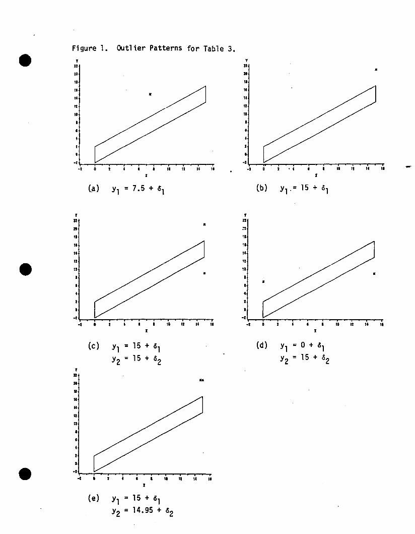
Figure I shows var.ious outlier patterns that might be of

interest. The "good" observations, simulated as above, are assumed

to lie in a pattern suggested by the parallelogram, and the symbol x

represents an outlier. Table 3 summarizes the results of the

simulations for each configuration of data in Fig. 1 in turn. Each

outlier is created by adding a quantity 6 to the x value(s) specified

in Fig. 1. The performance of the recursive method is then evaluated

in Table 3 for increasing 6. The entries in the table are as defined

before, using divisors chosen as in Table 2.

----Insert Figure 1 Here----

In Fig. l(a), the outlier occurs near the mean of the explanatory

variable. It can be seen that the power of the test gets very close

16

-

to 1 for 6 as small as 3. The outlier in Fig. l(b) is at the extreme of

the range of x. The power to detect this sort of outlier is less than

for .the first type, reflecting the greater impact of uncertainty in

estimation of the slope at x values farther from the mean X. In Fig.

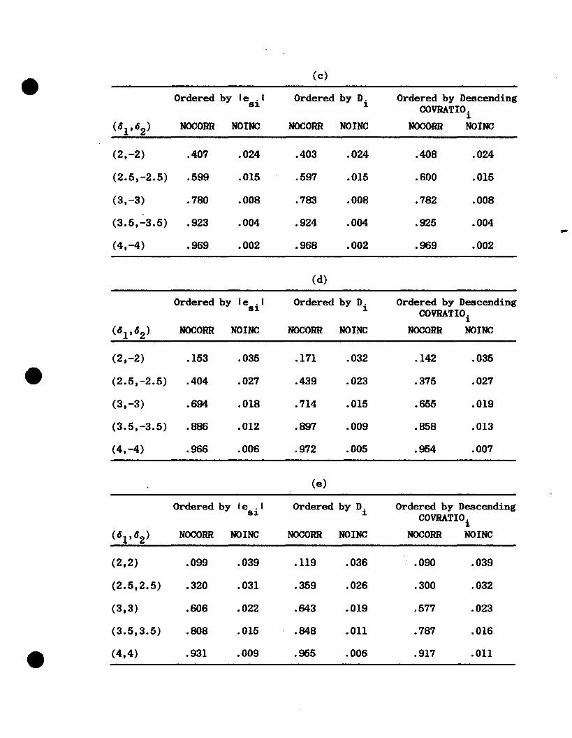
l(c), both outliers are at one extreme of the range of the x values,

with 6's of opposite signs. Power in this case suffers as the outliers

become more exaggera~d (larger 6's). This reflects the type of

masking discussed earlier wherein each outlier inflates the estimate of

variance, S2 (t), used in the denominator of the test statistic for the

other. In all the cases considered above [Figs. 1(a-c)], the choice of

the ordering variable does not make an appreciable difference in the

power of the recursive method. Ordering by D t appears to be

somewhat less effective in the first case, but this is the least

important case because (i) power is high and (ii) an undetected

outlier will have little influence on the estimate of the slope.

----Insert Table 3 Here---

Figure l(d) displays two outliers, one at each end of the range of

the explanatory variable and having «S's with opposite signs. Figure

l(e) has both outliers at the same end of the range and with 6's of

the same sign. Figures l(d) and 1(e) serve as examples where more

serious masking is found, that is, in which the presence of one

outlier is more likely to obscure the presence of another. Now, not

only does each outlier inflate the estimate of error used to test the

other, but also the first outlier in the ordered sample reduces the

17

-

size of the recursive residual for the second outlier through its

effect on ~j-l of (2.1). In the case in Fig. l(c), the first outlier

torqued the fitted line away from the second outlier, increasing its

recursive residual and thus "unmasking" it. In the cases in Figs.

l(d) and I(e), the line will be torqued toward the second outlier,

reducing its recursive residual and thereby the likelihood that it

will be identified as an outlier. For these two cases, Dt seems to be

superior to le.t I, which in turn is preferable to COVRATIOt for

ordering.

These simulation results suggest that the recursive method is

very effective in detecting outliers, although not equally so in all

cases. In practice, anyone of lest I or Dt or COVRATIO t that is

readily available can be used to rearrange the data before computing

the recursive residuals. The studentized. residual, e.t, is most widely

available and best-known; COVRATIO is least available and least

well-known. What differences we did observe, favor using Cook's D

as the ordering variable.

The above simulations explore the properties of the recursive

method per se. Kianifard and Swallow (North Carolina State

University, Institute of Statistics Mimeo Series No. 1906, 1988) compare

the recursive method with some competing outlier-detection

procedures. Two of these, testing the max Iest I of (1.3) or the

maxlt.1 of (1.4), are commonly seen in applications where there is no

a priori reason to suspect which observations, if any, might be

outliers. In each procedure, whenever the tested observation is

18

declared to be an outlier, that observation is deleted from the sample,

new e s t or tt are computed, the maximum tested, and so on. Both

procedures are known to be vulnerable to masking and swamping, but

the required computations are very manageable. A third competitor

in the comparison is Marasinghe's (1985) multistage procedure,

particularly designed for multiple-outlier applications.

Head-to-head comparisons of diagnostics or tests for identifying

outliers or influential observations are generally problematic, since

the competitors are often designed for somewhat different purposes,

and may test (somewhat) different hypotheses. That notwithstanding,

our principal conclusion is that the recursive method is generally

superior to these competitors for detecting moderate outliers

(c5's =3 or 4, or even 5 for some outlier configurations). If one

wants a procedure that has high probability of identifying these

moderate outliers for scrutiny and perhaps special treatment, the

recursive method seems a good choice. For a more detailed reporting

of this comparison, see Kianifard and Swallow.

5. An Example

We illustrate the use of recursive residuals in detecting outliers

on· a set of data from Brownlee (1965) that has been used extensively

in the literature. The data appear in Table 4. The observations

were ordered according to Ies t I obtained by fitting the regression

model to the data. Recursive residuals wJ were then computed and

scaled by S( t). The resulting IwJ/S( t) I shown in Table 4 are

compared to the percentiles of a t distribution with n-p-l = 16 df.

19

-

The appropriate critical value for testing at the 5% level is 2.120. It

can readily be seen from Table 4 that observations 21 and 4 are

identified as data points deserving further scrutiny and, perhaps,

special treatment. Experienced data analysts have applied a variety

of tools to identify outliers in this data set; their conclusions have

generally been that observations 21 and 4, and perhaps 1 and 3,

should be viewed as outliers.

----Insert Table 4 Here----

ACKNOWLEDGEMENTS

The programming assistance of Sandra B. Donaghy is greatly

appreciated by the authors. This research was partially supported

by the North Carolina Agricultural Foundation.

20

-

REFERENCES

Atkinson, A. C. (1981). Two Graphical Displays for Outlying and

Influential Observations in Regression. Biometrika 68, 13-20.

(1985). Plots, Transformations, and Regression. Oxford:

University Press.

Barnett, V., and Lewis, T. (1984) Outliers in Statistical Data,

Second Edition. New York: Wiley.

Belsley, D. A., Kuh, E., and Welsch, R. E. (1980). Regression

Diagnostics: IdentifTing Influential Data and Sources of

Collinearity. New York: Wiley.

Brown, R. L., Durbin, J., and Evans, J. M. (1975). Techniques for

Testing the Constancy of Regression Relationships over Time.

Journal of the Royal Statistical Society, Series B, 37, 149-192.

Brownlee, K. A. (1965). Statistical Theory and Methodology in

Science and Engineering, Second Edition. New York: Wiley.

Chatterjee, S., and Radi, A. S. (1986). Influential Observations,

High Leverage Points, and Outliers in Linear Regression.

Statistical Science 1, 379-416.

Chatterjee, S., and Radi, A. S. (1988). Sensitivity Analysis in Linear

Regression. New York: Wiley.

Cook, R. D. (1977). Detection of Influential Observations in Linear

Regression. Technometrics 19, 15-18.

Cook, R. D., and Weisberg, S. (1982). Residuals and Influence in

Regression. New York: Chapman and Hall.

21

-

Du Toit, S. H. c., St.eyn, A. G. W., and Stumpf, R. H. (1986). Graphical

Exploratory Data Analysis. New York: Springer-Verlag.

Galpin, J. S., and Hawkins, D. M. (1984). The Use of Recursive

Residuals in Checking Model Fit in Linear Regression. The

American Statistician 38, 94-105.

Harvey, A. C., and Collier, P. (1977). Testing for Functional

Misspecification in Regression Analysis. Journal of Econometrics

6, 103-109.

Harvey, A. C., and Phillips, G. D. A. (1974). A Comparison of the

Power ot Some Tests tor Heteroskedasticity in the General Linear

Model. Journal of Econometrics 2, 307-316.

Hawkins, D. M. (1980). Identification of Outliers. New York:

Chapman and Hall.

Hedayat, A., and Robson, D. S. (1970). Independent Stepwise Residuals

tor Testing Homoscedasticity. Journal of the American Statistical

Association 65, 1573-1581.

Marasinghe, M. G. (1985). A Multistage Procedure tor Detecting

Several Outliers in Linear Regression. Technometrics 27, 395-399.

Phillips, G. D. A., and Harvey, A. C. (1974). A Simple Test tor Serial

Correlation in Regression Analysis. Journal of the American

Statistical Association 69, 935-939.

Rousseeuw, P. J., and Leroy, A. M. (1987). Robust Regression and

Outlier Detection. New York: Wiley.

Plackett, R. L. (1950). Some Theorems in Least Squares. Biometrika

37, 149-157.

Theil, H. (1971). Principles of Econometrics, New York: Wiley.

22

-

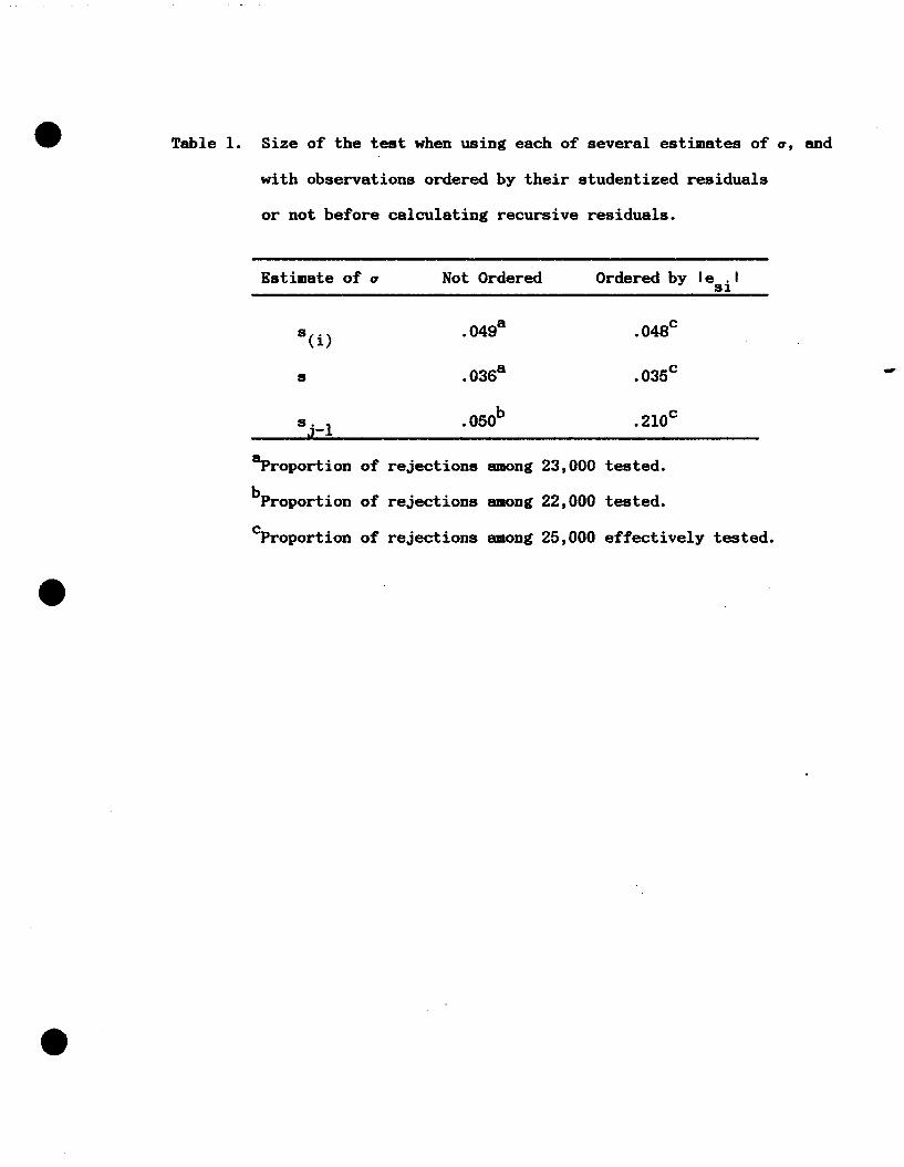
Table 1. Size of the test when using each of several estimates of a, and

with observations ordered by their studentized residuals

or not before calculating recursive residuals.

Estimate of a Not Ordered Ordered by Ie . IS1

s(i) .049a .048c

s .036a .035c

s. 1 .050b .2l0cJ-

Bproportion of rejections 8JDong 23,000 tested.

bproportion of rejections 8JDong 22,000 tested.

cProportion of rejections 8JDong 25,000 effectively tested.

Table 2. Proportions of outliers correctly identified (NOCORR) and nonoutliers

incorrectly declared to be outliers (NOINC) when up to three outliers

per sample were planted at randomly chosen x at (vertical) distances

6. from the true regression line, and the observations were not1

ordered, or ordered by their studentized residuals, or values of Cook's D

or the covariance ratio, before calculating recursive residuals.

OutlierPattern

NotOrdered

Orderedby Ie .1

S1

Orderedby D.

1

Ordered byDescending COVRATIO.

1

(2.5,0,0)

(3,0,0)

(4,0,0)

(3,3,0)

(3,3,-3)

NOCORR

.662

.848

.935

.703

.552

NOINC NOCORR

.03la .725

.025a .934

.015a .999

.015b .767

.007c .610

NOINC NOCORR

.029d .737

.022d .940

.ond .999

.015e .747

.008f .625

NOINC

.029d

.022d

.012d

.014e

.007f

NOCORR

.722

.929

.999

.757

.609

NOINC

.030d

.022d

.Olld

.016e

.008f

8proportion of rejections among 22,000 tested.

bproportion of rejections among 21,000 tested.

cProportion of rejections among 20,000 tested.

dproportion of rejections among 24,000 effectively tested.

~roportion of rejections among 23,000 effectively tested.

fproportion of rejections among 22,000 effectively tested.

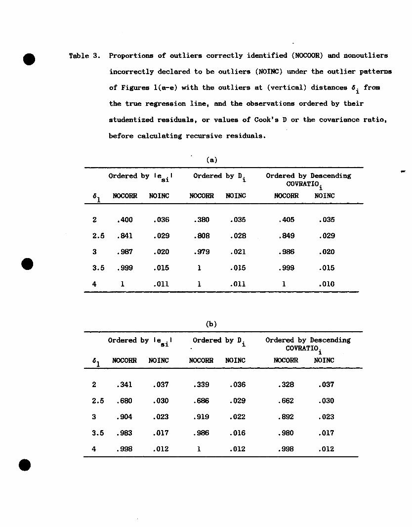
Table 3. Proportions of outliers correctly identified (NOCOOR) and nonoutliers

incorrectly declared to be outliers (NOINC) under the outlier patterns

of Figures l(a-e) with the outliers at (vertical) distances 6. from1

the true regression line, and the observations ordered by their

studentized residuals, or values of Cook's D or the covariance ratio,

before calculating recursive residuals.

(a)

-Ordered by Ie. I Ordered by D. Ordered by DescendingS1 1 COVRATIO.

1

61 NOCORR NOINC NOCORR NOINC NOCORR NOINC

2 .400 .036 .380 .035 .405 .035

2.5 .841 .029 .808 .028 .849 .029

3 .987 .020 .979 .021 .986 .020

3.5 .999 .015 1 .015 .999 .015

4 1 .011 1 .011 1 .010

(b)

Ordered by Ie. I Ordered by D. Ordered by DescendingS1 1 COVRATIO.

1

61 NOCORR NOINC NOCORR NOINC NOCORR NOINC

2 .341 .037 .339 .036 .328 .037

2.5 .680 .030 .686 .029 .662 .030

3 .904 .023 .919 .022 .892 .023

3.5 .983 .017 .986 .016 .980 .017

4 .998 .012 1 .012 .998 .012

(c)

Ordered by Ie. I Ordered by D. Ordered by DescendingSl. l. COVRATIO.

l.

( c5I' c52) NOCORR NOINe NOCORR NOINC NOCORR NOINe

(2,-2) .407 .024 .403 .024 .408 .024

(2.5,-2.5) .599 .015 .597 .015 .600 .015

(3,-3) .780 .008 .783 .008 .782 .008

(3.5,-3.5) .923 .004 .924 .004 .925 .004 -(4,-4) .969 .002 .968 .002 .969 .002

(d)

Ordered by Ie. I Ordered by D. Ordered by DescendingS1 1 COVRATIO.

1

( c5I' c52) NOCORR NOINC NOCORR NOINC NOCORR NOINe

(2,-2) .153 .035 .171 .032 .142 .035

(2.5,-2.5) .404 .027 .439 .023 .375 .027

(3,-3) .694 .018 .714 .015 .655 .019

(3.5,-3.5) .886 .012 .897 .009 .858 .013

(4,-4) .966 .006 .972 .005 .954 .007

(e)

Ordered by Ie. I Ordered by D. Ordered by DescendingS1 1 COVRATIO.

1

( c5I' c52) NOCORR NOINe NOCORR NOINC NOCORR NOINC

(2,2) .099 .039 .119 .036 .090 .039

(2.5,2.5) .320 .031 .359 .026 .300 .032

(3,3) .606 .022 .643 .019 .577 .023

(3.5,3.5) .808 .015 .848 .Oll .787 .016

(4,4) .931 .009 .955 .006 .917 .Oll

Table 4. Application of the recursive method to Brownlee's (1965) data

Data Ordered by Ie. IS1.

Observation Xl X2 X3 Y wj/s(i) ObservationNumber Number

1 .80 27 89 42 0 14

2 80 27 88 37 0 18

3 75 25 90 37 0 19

-4 62 24 87 28 0 16

5 62 22 87 18 .1753 10

6 62 23 87 18 .4278 20

7 62 24 93 19 -.6332 13

8 62 24 93 20 -.2210 8

9 58 23 87 15 -.2533 5

10 58 18 80 14 -.3511 17

11 58 18 89 14 .1802 2

12 58 17 88 13 .5093 15

13 58 18 82 11 -.3775 7

14 58 19 93 12 .4507 11

15 50 18 89 8 -.4720 6

16 50 18 86 7 .2152 12

17 50 19 72 8 -.3596 9

18 50 19 79 8 1.5019 1

19 50 20 80 9 1.3020 3

20 56 20 82 15 2.2758 4

21 70 20 91 15 -3.3305 21

Y = stack loss Xl = air flow

X2 = cooling water inlet temperature X3 = acid concentration

..

t.

2

•-2

10 It 14 11 -t • • • II 12 It 11I

(d) Y1 = o + 151Y2 = 15 + 152

-I -.-2 0 10 12 11 11 -t • I 10 IZ It 11 -

I I

Ca) Y1 = 7.5 + 51 (b) Y1.= 15 + 151

, ,II J2•ZI :1

"~.

II ~.

It tt

11 lZ

" 11

-I

-t •

(c) Y1 = 15 + 151Y2 = 15 + 15 2,

II

21

II

"It

12

10

•-t

-t • • • "12 14 11

I

(e) Y1 = 15 + 151Y2 = 14.95 + 152

Figure 1- Outlier Patterns for Table 3., ,

12 12•Z, ZI

",.

11 11 :J11 11

12,.

10 11