Using Phylogenetic Trees for Disease Diagnosis

Dissertation

submitted in partial fulfillment of the requirements

for the degree of

Master of Technology, Computer Engineering

by

Shamsudduha Tabish M Sabir Danish

Roll No:121122018

under the guidance of

Mr. Satish S Kumbhar

College of Engineering, Pune

DEPARTMENT OF COMPUTER ENGINEERING AND

INFORMATION TECHNOLOGY,

COLLEGE OF ENGINEERING, PUNE-411005

June, 2013

DEPARTMENT OF COMPUTER ENGINEERING AND

INFORMATION TECHNOLOGY,

COLLEGE OF ENGINEERING, PUNE

CERTIFICATE

This is to certify that the dissertation titled

Using Phylogenetic Trees for Disease Diagnosis

has been successfully completed

By

Shamsudduha Tabish M Sabir Danish

(121122018)

and is approved for the degree of

Master of Technology in Computer Engineering.

Date: June 2013. Prof. Satish S. Kumbhar

Place:Pune Department of Computer Engg.

and Information Technology,

College of Engineering Pune,

Shivajinagar, Pune - 411005.

Dedicated to

my Mother

Smt.Mudassir Danish

and

my father

Shri. M. Sabir Danish

Abstract

The Phylogenetic Tree is a tool for tracking the evolution process by looking into the changes in the

genome sequences under study. This tree is a graphical representation of the evolutionary relationships

among multiple genes or organisms. In this work we apply the this principle of phylogeny to diagnose

what disease an individual is suffering from. In our method the multiple sequence alignment is applied to

a set of omic (Genomic or Proteomic) sequences of the patient, a few family members of the patient and

the diseased sequences or reference sequences. Once we get the result of Multiple Sequence Alignment,

the similarity in the omic sequences of patients family members is found along with the loci of each com-

mon nucleotide/amino acid, and the dissimilar nucleotides or amino acid at respective loci are discarded

also from the patients and diseased sequences. Finally we create a phylogenetic tree from these sequences

which can now be used to visualize the distance among the patients genome sequence and the diseased

genome sequences. After applying this algorithm on the data available at the 1000 genome project and

dbSNP we got the expected ressults and hence the algorithms is proved for the accuracy.

Keywords: Disease diagnosis, evolution, medical diagnosis, Phylograms, cladograms, Phylogenetic

trees, Multiple Sequence Alignment.

Acknowledgments

I would like to take this opportunity to express my gratitude towards my guide Prof. Satish S Kumb-

har for his constant help and suppoert, encouragement and inspiration for the project work. Without

his invaluable guidance, this work would never have been a reached to this level. I would also like to

thank all the faculty members and staff of Computer and IT department for providing us ample facility

and flexibility and for making my journey of post-graduation successful.

Last, but not the least, I would like to thank my classmates for their valuable suggestions and helpful

discussions. I am thankful to them for their unconditional support and help throughout the year.

Shamsudduha Tabish

College of Engineering, Pune.

ii

Contents

Abstract ii

Acknowledgements i

List of Figures v

1 Introduction 1

1.1 DNA ( Deoxyribo Nucleic Acid ) . . . . . . . . . . . . . . . . . . . . . . . . . . . . . . . . 2

1.2 SNP (Single Nucleotide Polymorphism) . . . . . . . . . . . . . . . . . . . . . . . . . . . . 2

1.3 Mutation . . . . . . . . . . . . . . . . . . . . . . . . . . . . . . . . . . . . . . . . . . . . . 5

1.3.1 Mutagens . . . . . . . . . . . . . . . . . . . . . . . . . . . . . . . . . . . . . . . . . 5

1.3.2 Chemical Mutagens . . . . . . . . . . . . . . . . . . . . . . . . . . . . . . . . . . . 5

1.3.3 Radiation . . . . . . . . . . . . . . . . . . . . . . . . . . . . . . . . . . . . . . . . . 6

1.3.4 Sunlight . . . . . . . . . . . . . . . . . . . . . . . . . . . . . . . . . . . . . . . . . . 6

1.3.5 Spontaneous mutations . . . . . . . . . . . . . . . . . . . . . . . . . . . . . . . . . 6

2 Literature Survey 7

2.1 Problem statement . . . . . . . . . . . . . . . . . . . . . . . . . . . . . . . . . . . . . . . . 7

2.2 Multiple Sequence Alignment (MSA) . . . . . . . . . . . . . . . . . . . . . . . . . . . . . . 8

2.3 Phylogenetic Trees . . . . . . . . . . . . . . . . . . . . . . . . . . . . . . . . . . . . . . . . 8

2.4 Constructing Phylogenetic Trees . . . . . . . . . . . . . . . . . . . . . . . . . . . . . . . . 11

2.4.1 Distance Methods . . . . . . . . . . . . . . . . . . . . . . . . . . . . . . . . . . . . 11

2.4.2 Character Based Methods . . . . . . . . . . . . . . . . . . . . . . . . . . . . . . . . 14

2.4.3 Maximum Likelihood . . . . . . . . . . . . . . . . . . . . . . . . . . . . . . . . . . . 17

3 Data Sets 18

3.1 The HapMap Project . . . . . . . . . . . . . . . . . . . . . . . . . . . . . . . . . . . . . . . 18

3.2 dbSNP . . . . . . . . . . . . . . . . . . . . . . . . . . . . . . . . . . . . . . . . . . . . . . . 19

3.3 The 1000 Genomes Project . . . . . . . . . . . . . . . . . . . . . . . . . . . . . . . . . . . 19

4 Technologies 20

4.1 Tomcat Server . . . . . . . . . . . . . . . . . . . . . . . . . . . . . . . . . . . . . . . . . . 20

4.2 Web Services . . . . . . . . . . . . . . . . . . . . . . . . . . . . . . . . . . . . . . . . . . . 20

iii

4.3 JSP (Java Server Pages) . . . . . . . . . . . . . . . . . . . . . . . . . . . . . . . . . . . . . 21

4.4 HTML 5 . . . . . . . . . . . . . . . . . . . . . . . . . . . . . . . . . . . . . . . . . . . . . . 21

4.5 Java Script . . . . . . . . . . . . . . . . . . . . . . . . . . . . . . . . . . . . . . . . . . . . 21

4.6 Eclipse . . . . . . . . . . . . . . . . . . . . . . . . . . . . . . . . . . . . . . . . . . . . . . . 22

5 DiagnosTree -The Tool 23

5.1 The Algorithm . . . . . . . . . . . . . . . . . . . . . . . . . . . . . . . . . . . . . . . . . . 23

5.1.1 Required Inputs . . . . . . . . . . . . . . . . . . . . . . . . . . . . . . . . . . . . . 23

5.1.2 Example . . . . . . . . . . . . . . . . . . . . . . . . . . . . . . . . . . . . . . . . . . 24

6 System Architecture 27

7 Results 30

8 Conclusion 31

9 Future Work 32

List of Figures

1.1 The Eukaryotic Cell Structure . . . . . . . . . . . . . . . . . . . . . . . . . . . . . . . . . . 1

1.2 The DNA Composition and Structure . . . . . . . . . . . . . . . . . . . . . . . . . . . . . 3

1.3 The Chemical Structures of Cytosine, Thymine, Adenine and Guanine . . . . . . . . . . . 4

2.1 A Phylogeny of Six Species . . . . . . . . . . . . . . . . . . . . . . . . . . . . . . . . . . . 9

2.2 Rooted and Unrooted Trees . . . . . . . . . . . . . . . . . . . . . . . . . . . . . . . . . . . 10

2.3 Example: A distance Matrix M . . . . . . . . . . . . . . . . . . . . . . . . . . . . . . . . . 11

2.4 Unrooted tree from the given matrix of M nodes . . . . . . . . . . . . . . . . . . . . . . . 12

2.5 Comparison of two sequences with their ancestor shows several types of substitutions . . . 13

2.6 Set of Input sequences for Maximumparsimony Algorithm . . . . . . . . . . . . . . . . . . 14

2.7 Trees for first two sites of sequences A through E . . . . . . . . . . . . . . . . . . . . . . . 15

2.8 Pictorial Example Employing Fitch’s Algorithm for given site . . . . . . . . . . . . . . . . 16

2.9 Choosing the right algorithm that suits your needs . . . . . . . . . . . . . . . . . . . . . . 17

5.1 Set of Input Sequences . . . . . . . . . . . . . . . . . . . . . . . . . . . . . . . . . . . . . . 24

5.2 Aligned Sequences (Output of MSA) . . . . . . . . . . . . . . . . . . . . . . . . . . . . . . 25

5.3 Uncommon Nucleotieds to be omitted out of the sequences . . . . . . . . . . . . . . . . . 25

5.4 Set of Family Members Sequences to be removed from The Sequences . . . . . . . . . . . 26

5.5 Final set of Sequences to be used for creating The Phylogenetic Tree . . . . . . . . . . . . 26

5.6 The resultant Tree depicting relationship among the patients gene sequence and different

diseased sequences . . . . . . . . . . . . . . . . . . . . . . . . . . . . . . . . . . . . . . . . 26

6.1 Layered System Architecture . . . . . . . . . . . . . . . . . . . . . . . . . . . . . . . . . . 27

6.2 Component Based System Architecture . . . . . . . . . . . . . . . . . . . . . . . . . . . . 28

6.3 Flowchart for the Algorithm . . . . . . . . . . . . . . . . . . . . . . . . . . . . . . . . . . . 29

v

Chapter 1

Introduction

Our work is completely based on the DNA/RNA/Protein found in the cell of almost all the living

organisms. To understand these elements lets get into the cell and find out where they are created and

what role do they play. The basic b building block of every living being on this planet is biologic al cell.

The Cell is composed of Nucleus, Mitochondria, cytoplasm, etc. There are two types of cells, prokaryotic

and eukaryotic cells. Most of single cellular organisms are made up of prokaryotic cells (eg. Bacteria),

where as the all the multi-cellular organisms are made up of eukaryotic cells. In this work we focus on

eukaryotic cellular organisms.

Figure 1.1: The Eukaryotic Cell Structure

The above figure 1.1 shows the structure of a cell in eukaryotic organism. The DNA is found in

1

almost every living organism. The chromosomes are composed of DNA and are found in the cell. The

Nucleus in the above figure 1.1 is the main part of the cell containing large amount of DNA, only a small

portion of the DNA is found in the Mitochondrion as shown in the figure. This DNA is called as mtDNA

or Mitochondrion DNA. The DNA is the code which encodes everything about the organism including

the behavior, appearance, diseases, resistance to diseases and every character an organism posses.

1.1 DNA ( Deoxyribo Nucleic Acid )

DeoxyriboNucleic Acid (DNA) is the hereditary material found in almost all living organisms. Nearly

every cell in the human body has exactly the same replica of DNA. Most of the DNA is located in the

nucleus of the call (called nuclear DNA), but a small amount of DNA is also be found in mitochondria

(mitochondrial DNA or mtDNA).

The DNA is composed of two strands having backbone madeup of phosphorous group and pentose

sugar. These strands are connected to each other by adenine (A), guanine (G), cytosine (C), and thymine

(T) as shown in the figure. The Human DNA has about 3 billion base pairs, and more than 99% of

those bases are the same in all human beings. The sequence of these bases determine the information

for building and maintaining an organism, in a similar way in which letters of the alphabet are arranged

in a certain order to form words and sentences.

The DNA bases, pair up with each other, A pairs with T and C pairs with G, to form units which

are called base pairs. Each base is also attached to a sugar molecule and a phosphate molecule which are

together the backbone for DNA. A base, sugar, and phosphate together are called a nucleotide. These

nucleotides are arranged in two long sequences called strands that together form a spiral called a double

helix. The structure of the double helix looks like a ladder, where the base pairs form the ladders rungs

and the sugar and phosphate molecules form the vertical sidepieces of the ladder but in a spiral form.

The figure 1.2 shows the chemical structure of DNA as explaind in the forth coming description and

figure 1.3 shows the chemical structure of the different nucleotides playing a vital role in the structure

and composition of DNA. Only because of these chemical compounds the DNA has the two strands

connected and a spiral shape.

1.2 SNP (Single Nucleotide Polymorphism)

Single Nucleotide Polymorphism also known as SNP (Snip) is a change of single nucleotide in the genome

a particular locus. If such a variation at a single locus is found common in more than 1% of the population,

only then it is considered as SNP. Around 90% of the variation in the genome is because of SNPs. SNPs

are scattered across the human genome by an approximate average of one SNP per thousand base pairs,

these SNPs directly affect the gene product that is the protein. Sequence variations in the genomes exist

at defined positions and are responsible for phenotypic characteristics, including a person’s tendency

towards complex diseases like heart disease and cancer.

Single nucleotide polymorphisms, frequently called SNPs (pronounced snips), are the most common

2

Figure 1.2: The DNA Composition and Structure

type of genetic variation among people. Each SNP represents a difference in a single DNA building block,

called a nucleotide. For example, a SNP may replace the nucleotide cytosine (C) with the nucleotide

thymine (T) in a certain stretch of DNA.

SNPs occur normally throughout a persons DNA. More precisely, they occur once in every 300

nucleotides on average, which means there are roughly 10 million SNPs in the human genome. Most

commonly, these variations are found in the DNA between genes. They can act as biological markers,

helping scientists locate genes that are associated with disease. When SNPs occur within a gene or in a

regulatory region near a gene, they may play a more direct role in disease by affecting the genes function.

Most SNPs have no effect on health or development. Some of these genetic differences, however, have

proven to be very important in the study of human health. Researchers have found SNPs that may help

predict an individuals response to certain drugs, susceptibility to environmental factors such as toxins,

and risk of developing particular diseases. SNPs can also be used to track the inheritance of disease

genes within families. There is a scope for future studies for identifying SNPs associated with complex

diseases such as heart disease, diabetes, and cancer.

At present there are a number of SNP analysis techniques available, some of these methods are

inefficient and others require manual intervention. Using a 5’ nuclease assay chemistry protocol is a fast

and simple way to get data results. The experiment protocol involves combining purified genomic DNA,

3

Figure 1.3: The Chemical Structures of Cytosine, Thymine, Adenine and Guanine

master mix, and a 5’ nuclease assay, then thermal cycling, reading, and analyzing the results.

For example a SNP might change the DNA sequence AAGGCTAA to ATGGCTAA. For a variation

to be considered a SNP, it must occur in at least 1% of the population. SNPs, which make up about

90% of all human genetic variation, occur every 100 to 300 bases along the 3-billion-base human genome.

Two of every three SNPs involve the replacement of cytosine (C) with thymine (T). SNPs can occur in

coding (gene) and non-coding regions of the genome. Many SNPs have no effect on cell function, but

scientists believe others could predispose people to disease or influence their response to a drug.

Although more than 99% of human DNA sequences are the same, variations in DNA sequence can

have a major impact on how humans respond to disease, environmental factors such as bacteria, viruses,

toxins, and chemicals and drugs and other therapies. This makes SNPs valuable for biomedical research

and for developing pharmaceutical products or medical diagnostics. SNPs are also evolutionarily stable

that is not changing much from generation to generation which make them easier to follow in population

studies. Scientists believe SNP maps will help them identify the multiple genes associated with complex

ailments such as cancer, diabetes, vascular disease, and some forms of mental illness. These associations

are difficult to establish with conventional gene-hunting methods because a single altered gene may make

only a small contribution to the disease.

Several previous contributions to find SNPs and ultimately create SNP maps of the human genome.

Among these were the U.S. Human Genome Project (HGP) and a large group of pharmaceutical compa-

nies called the SNP Consortium or TSC project. The likelihood of duplication among the groups is small

because of the estimated 3 million SNPs, and the potential payoff of a SNP map was high. In addition

to pharmacogenomic, diagnostic and biomedical research implications, SNP maps are being utilized to

identify thousands of additional markers in the genome, thus simplifying navigation of the much larger

genome map generated by HGP researchers. SNPs as risk factors in disease development SNPs do not

cause disease, but they can help determine the likelihood that someone will develop a particular illness.

One of the genes associated with Alzheimer’s disease, apolipoprotein E or ApoE, is a good example of

how SNPs affect disease development. ApoE contains two SNPs that result in three possible alleles for

this gene: E2, E3, and E4. Each allele differs by one DNA base, and the protein product of each gene

differs by one amino acid.

Each individual inherits one maternal copy of ApoE and one paternal copy of ApoE. Research has

4

shown that a person who inherits at least one E4 allele will have a greater chance of developing Alzheimer’s

disease. Apparently, the change of one amino acid in the E4 protein alters its structure and function

enough to make disease development more likely. Inheriting the E2 allele, on the other hand, seems to

indicate that a person is less likely to develop Alzheimer’s. Of course, SNPs are not absolute indicators of

disease development. Someone who has inherited two E4 alleles may never develop Alzheimer’s disease,

while another who has inherited two E2 alleles may. ApoE is just one gene that has been linked to

Alzheimer’s. Like most common chronic disorders such as heart disease, diabetes, or cancer, Alzheimer’s

is a disease that can be caused by variations in several genes. The polygenic nature of these disorders is

what makes genetic testing for them so complicated.

1.3 Mutation

A Mutation occurs when a DNA gene is damaged or changed in such a way as to alter the genetic

message carried by that gene.

A Mutagen is an agent of substance that can bring about a permanent alteration to the physical

composition of a DNA gene such that the genetic message is changed.

Once the gene has been damaged or changed the mRNA transcribed from that gene will now carry

an altered message. The polypeptide made by translating the altered mRNA will now contain a different

sequence of amino acids. The function of the protein made by folding this polypeptide will probably be

changed or lost. In this example, the enzyme that is catalyzing the production of flower color pigment

has been altered in such a way it no longer catalyzes the production of the red pigment.

No product (red pigment) is produced by the altered protein. In subtle or very obvious ways, the

phenotype of the organism carrying the mutation will be changed. In this case the flower, without the

pigment is no longer red.

1.3.1 Mutagens

A Mutagen is an agent of substance that is responsible for permanent alteration to the physical compo-

sition of a DNA such that the genetic message is changed. Such a change may impact the organism on

its physical appearance or in the other way which may not be directy visible.

1.3.2 Chemical Mutagens

change the sequence of bases in a DNA gene in a number of ways;

• It mimics the correct nucleotide bases in a DNA molecule, but fail to base pair correctly during

DNA replication.

• Remove parts of the nucleotide (such as the amino group on adenine), again causing improper base

pairing during DNA replication.

• Add hydrocarbon groups to various nucleotides, also causing incorrect base pairing during DNA

replication.

5

1.3.3 Radiation

High energy radiation from a radioactive material or from X-rays is absorbed by the atoms in water

molecules surrounding the DNA. This energy is transferred to the electrons which then fly away from

the atom. Left behind is a free radical, which is a highly dangerous and highly reactive molecule that

attacks the DNA molecule and alters it in many ways. Radiation can also cause double strand breaks in

the DNA molecule, which the cell’s repair mechanisms cannot put right.

1.3.4 Sunlight

contains ultraviolet radiation (the component that causes a suntan) which, when absorbed by the DNA

causes a cross link to form between certain adjacent bases. In most normal cases the cells can repair

this damage, but unrepaired dimmers of this sort cause the replicating system to skip over the mistake

leaving a gap, which is supposed to be filled in later. Unprotected exposure to UV radiation by the

human skin can cause serious damage and may lead to skin cancer and extensive skin tumors.

1.3.5 Spontaneous mutations

occur without exposure to any obvious mutagenic agent. Sometimes DNA nucleotides shift without

warning to a different chemical form (know as an isomer) which in turn will form a different series of

hydrogen bonds with it’s partner. This leads to mistakes at the time of DNA replication.

6

Chapter 2

Literature Survey

The current diagnosis methods are mostly based on the non genetic tests, which involve blood test,

urine test, thyroid test, stool test, saliva test etc, all of these look into the chemicals and microbes

found in their respective inputs. And X-Ray, MRI, CT scan, ultra sound etc, look for the physical

appearance and functioning of the organs. Whereas Electroencephalography (EEG), Electrocardiogram

(ECG) also known as Electrocardiography (EKG), Electromyography (EMG) etc, look into the accuracy

of functioning of the organs. So these tests may or may not be successful in diagnosis of disease also a

combination of such tests is required to reach the actual cause of the disease.

Another new method that is on its way is through the analysis of human genome. For this method the

patients genome needs to be sequenced. Then it is compared using Multiple Sequence Analysis (MSA)

with the other reference genome of diseased people known to be suffering from a particular disease, if the

similarity is found then patient is diagnosed to be suffering from the disease of most similar sequence in

the set of input, but this requires a long time, in order to cut short this time we propose our method to

be used for the diagnosis.

2.1 Problem statement

Many a times doctors come across a situation where the diagnosis of a disease (a patient is suffering

from) become quite difficult and this diagnosis process may take months of time, and during this time

the patient is given treatment based on assumptions, if the assumptions go wrong then the patient has

to take drugs targeted for the disease he/she is not suffering from. Such drugs may leave heavy side

effects. Hence its the requirement of the medical system to speed up the diagnosis process and increase

its accuracy.

To this end, a modern technique which employ genome sequencing has been discovered lately for

efficient diagnosis of diseases. In this method the patients genome is sequenced first and is then compared

with the reference sequences. Although existing methods offer good accuracy but are a bit slow. This

motivates a need for a faster yet accurate method to diagnose the diseases.

7

2.2 Multiple Sequence Alignment (MSA)

Multiple Sequence Alignment (MSA) is the alignment of multiple biological sequences (of protein

or nucleic acid) of equal length. From the output of the multiple sequence alignment homology is inferred

and the evolutionary relationships between the sequences can be studied by creating Phylogenetic Trees.

Multiple Sequence Alignment (MSA) is usually the alignment of three or more nitrogen base se-

quences or Nucleic acid sequences of similar length. Homology can be inferred from the output and the

evolutionary relationships between the sequences studied. Usually protein sequences are aligned using

multiple sequence alignment to find out the relationship among them. The multiple sequence alignment

tools compare these sequences and try to correlate each other by introducing gaps in the sequences in

order to match these sequences.

A multiple sequence alignment arranges protein or nucleotide sequences into a rectangular array with

the goal that residues in a given column are homologous (that is they are derived from a single ancestral

sequence), and in a rigid local structural alignment or play a common functional role. Although these

criteria are essentially equivalent for closely related proteins (most similar sequences of amino acids),

structure and function diverge over evolutionary time sequences, and different criteria may result in

different alignments of these sequences.

Most of the existing tools do not meet the efficiency / precision expectations because the length of

these sequences is very high, and a complex algorithm is required to accurately align these sequences

and hence continuous efforts are being put in to improve the method. Such an algorithms require a

huge amount of RAM and processing power because of the nature of the input and complex algorithms

involved for getting a solution. Homology is the similarity that is the result of inheritance from a common

ancestor, and identification and analysis of homologies is central to phylogenetic systematics.

An Alignment is an hypothesis of positional homology between bases/Amino Acids.

Many tools exist for finding the MSA of given set of omic sequences, namely: Clustalw2 Clustal

Omega from EBI UK, T-COFFEE from Lausanne Switzerland, VRIJE universitys PARALINE, bioin-

formatics.orgs STRAP, MAFFT from Tokyo, Japa, MUSCLE from EBI UK, and many more. We have

chosen the popular EMBL EBIs Clustal Omega for multiple sequence alignment in our work. Almost all

these tools are based on dynamic programming.

2.3 Phylogenetic Trees

A phylogenetic tree is described as, a branching diagram that shows, for each species, with which other

species it shares its most recent common ancestor. The evolutionary tree or cladograms were traditionally

used to draw evolutionary relationship among the organism; a more modern version of the same is phylo-

genetic tree which uses gene / protein sequences to draw the evolutionary relationship. These trees dictate

the relationship among the organisms based on the similarity and dissimilarity among the nucleotide or

nucleic acid sequences.

The tree construction can be done through variety of tree-building methods which include methods

8

based on distances, likelihood and characters. After a phylogenetic tree is constructed, it is important

to test its accuracy which refers to the degree to which a tree is close to the true tree.

Phylogenetics is the study of evolutionary relationships among organisms or genes. Below, we will

refer to the objects whose phylogeny we are studying as organisms or species, but the discussion of

methods is valid for the phylogeny of genes as well. We construct phylogenetic trees to illustrate the

evolutionary relationships among a group of organisms. The purpose of phylogenetic studies are (1)

to reconstruct evolutionary ties between organisms and (2) to estimate the time of divergence between

organisms since they last shared a common ancestor.

There are several types of data that can be used to build phylogenetic trees: Traditionally, phylo-

genetic trees were built from morphological features (e.g., beak shapes, presence of feathers, number of

legs, etc). Today, we use mostly molecular data like DNA sequences and protein sequences. A phy-

logeny example showing the evolutionary history of six species: Fish, Deer, Cow, Human, Monkey and

Chimpanzee is shown in Figure 2.1.

Figure 2.1: A Phylogeny of Six Species

Each of the organism has discrete characters each character has a finite number of states. For

example, discrete characters include the number of legs of an organism, or a column in an alignment of

DNA sequences. In the latter case, the number of states for the column character is 4 (A, C, T, G).

Comparative Numerical Data These data encode the distances between objects and are usually derived

from sequence data. For example, we could hypothetically say distance (man, mouse) = 500 and distance

(man, chimp) = 100.

External nodes are things under comparison, also called operational taxonomic units (OTUs). Internal

nodes are hypothetical ancestral units. They are used to group current-day units. In rooted trees, the root

is the common ancestor of all OTUs under study. The path from root to a node defines an evolutionary

path. An unrooted tree specifies relationships among OTUs but does not specify evolutionary paths

9

Figure 2.2: Rooted and Unrooted Trees

(Figure 2.2). We can root an unrooted tree by finding an outgroup (i.e., if we have some external reason

indicating that a certain OTU branched off first). For example, in Figure 2.2, the unrooted tree can be

transformed to the rooted tree by making E the outgroup.

The topology of a tree is the branching pattern of a tree. All internal nodes of a bifurcating tree

have 2 descendants if it is rooted or 3 neighbors if it is unrooted. It is sometimes useful to allow more

than 2 descendants (or more than 3 neighbors in the unrooted case), but we will focus on bifurcating

trees. The branch length can represent the number of changes that have occurred in that branch, or can

indicate the genetic distance between nodes connected by that branch, or can indicate the amount of

evolutionary time passed along the branch.

In every phylogenetic tree, a time axis is implicit. In our example, the time at C is more recent than

the time at B which is in turn more recent than that at A. In this phylogeny, it shows that monkey and

chimpanzee had the most recent common ancestor at the time C. Then, some time before this, at time

B, the most recent common ancestor of human, monkey and chimpanzee were found. Finally, the most

recent common ancestor of all six species was found at time A.

Phylogeny inference can be used for analysis of sequences of proteins and DNA. The concept of

phylogeny is extended to haplotype sequences. The sequences of the individuals replace the species in

the phylogenetic tree. In this case, the phylogeny shows the evolutionary history of the individuals. This

concept also makes sense for sequences coming from the same individual, as in our case of using phylogeny

for reconstructing the haplotype sequences from genotypes. This is because the two sequences of the

individual actually come from his/her father and mother. The phylogeny shows the common ancestor of

both father and mother of the individuals. In our algorithm, we further extend the concept of phylogeny

and use it to represent only a column of the set of haplotype sequences. In every phylogenetic tree,

a time axis is implicit. In our example, the time at C is more recent than the time at B which is in

turn more recent than that at A. In this phylogeny, it shows that monkey and chimpanzee had the most

recent common ancestor at the time C. Then, some time before this, at time B, the most recent common

10

ancestor of human, monkey and chimpanzee were found. Finally, the most recent common ancestor of

all six species was found at time A.

2.4 Constructing Phylogenetic Trees

The three major methods for constructing phylogenetic trees are:

• Distance methods: Evolutionary distances are computed for all OTUs and these are used to

construct trees.

• Maximum Parsimony: The tree is chosen to minimize the number of changes required to explain

the data.

• Maximum Likelihood: Under a model of sequence evolution, the tree which gives the highest

likelihood of the given data is found.

2.4.1 Distance Methods

The problem can be described as follows:

Input: Given an n X n matrix M where Mij ≥ 0 and Mij is the distance between objects i and j.

Goal: Build an edge-weighted tree where each leaf corresponds to one object of M, and such that the

distances measured on the tree between leaves i and j correspond exactly to the value of Mij . When

such a tree can be constructed, we say the distances in M are additive.

Example: Suppose we are given the distances as in Table below.

Figure 2.3: Example: A distance Matrix M

Distance methods do not use the actual molecular sequence alignment during the tree inference but

calculate a symmetric n X n matrix from the input alignment in the beginning. The entries of this matrix

are the pair-wise-distances of the n sequences. The actual tree inference is then performed solely on the

basis of this matrix. n provides a measure for the genetic distance of each pair of the n sequences in the

input alignment. In the simplest case this function would only count the number of differing characters

of the two sequences. More elaborate functions, however, utilize a sophisticated model of molecular

11

Figure 2.4: Unrooted tree from the given matrix of M nodes

evolution. The most frequently used distance-based approaches are probably the LS (Least-Squares)

method and the UPGMA (Un-weighted Pair Group Method with Arithmetic Mean) and NJ (Neighbor-

Joining) heuristics.

Least-Squares

The Least-Squares method estimates the branch lengths of a tree topology by matching the distances

described by them as closely as possible to the values of the pair-wise distances matrix. This is achieved by

minimizing the sum of squared differences between the given (by the distances matrix) and the predicted

distances. The predicted distance between two sequences is calculated as the sum of the branch lengths

along the path connecting both of them. The sum of all squared differences represents a measure for

the fit of the tree to the given sequence data: the tree with the minimal sum is the optimal tree. The

complexity of LS is O(n3).

UPGMA

UPGMA is a clustering algorithm that builds a rooted tree topology by stepwise addition. A molecular

clock is assumed for the evolutionary process, which means that all species contained in the phylogenetic

tree are supposed to evolve at the same rate. This assumption leads to the fact that trees obtained by

UPGMA are ultra metric trees, that is, all end nodes (representing the species of interest) are equidistant

from the root.

The algorithm works as follows: In the beginning, each node represents a cluster. At each step,

the two clusters whose associated sequences have minimal distance according to the distance matrix

are joined. Their entries are removed from the matrix and an entry for the new cluster is added. The

distance of the new cluster to other clusters is computed as the mean distance of the sequences contained

in each cluster. The algorithm terminates when all clusters have been joined into a single cluster. The

complexity of UPGMA is O(n2).

Neighbor-Joining

Neighbor-Joining is also a clustering algorithm and is based on the minimum-evolution criterion. The

tree that explains the sequence data with the minimal amount of change, i.e., the tree which minimizes

the sum of all branch lengths (the total tree length), is the optimal tree. The algorithm starts with a

12

star-tree. At each step, two nodes are removed from the tree and reconnected via a common newly added

internal node. The distance of both nodes to any other node of the tree (i.e., the sum of the branch

lengths on the path connecting the nodes) stays constant. Yet, the total tree length is reduced as two

rather long branches are replaced by three shorter branches. The nodes to be reorganized are selected

such that the greatest reduction of the tree length is achieved. This procedure is repeated until the tree

is fully resolved. The complexity of the original NJ implementation is O(n3) which can be reduced to

O(n2) by using a more sophisticated algorithm for selecting the nodes to be joined.

Computing Distances

We have looked at a couple of distance method heuristics for reconstructing trees, given distance

data. One question we could ask at this point is: how do we obtain the distance data? One answer is

that distance data can be obtained from sequence data. Let us compare the following two sequences:

Figure 2.5: Comparison of two sequences with their ancestor shows several types of substitutions

There are only 3 observed difference between the 2 sequences; however, considering the ancestral

sequence, we see that are actually 12 total substitutions. Thus, if multiple substitutions have occurred

at any site (e:g:, the convergent substitution at site 11), then the naive way of computing distance is an

underestimate. How can we correct for multiple substitutions? For DNA sequences, we can use models

for nucleotide substitution. For protein sequences, we have already talked about models for amino acid

substitution in our discussion of PAM matrices. (We will also use these models when we talk about

maximum likelihood methods for phylogenetic reconstruction.)

13

2.4.2 Character Based Methods

Discrete characters include morphological data (such as the absence or presence of feathers), protein

data (20 possible amino acids), and DNA data (four possible nucleotides). All character based methods

assume that different characters are independent of each other. Given character data, how does one find

a tree out of the given data? What criteria are used to pick the best tree?

Maximum Parsimony

One method is to use maximum parsimony. In this instance, we want to find the tree that minimizes

the number of changes needed to explain the data. For example, given the following DNA data, which

tree is most parsimonious?

Figure 2.6: Set of Input sequences for Maximumparsimony Algorithm

Sites 1 and 2 each require one change for the given tree. It turns out that the entire data can be

explained with a minimum of 9 changes using the tree in Figure below. However, changing the tree will

alter the minimum number of changes required. This example leads us to ask two important questions

relating to parsimony:

• Given a particular tree, how do you find the minimum number of changes needed to explain the

data? (Easy)

• How do you find the most parsimonious tree? (NP-hard)

To answer the easy first question, we use Fitch’s Algorithm. The idea is to construct a set of possible

states (eg: nucleotides) for internal nodes based on the states of the children. For each site, each leaf is

labeled by a singleton set containing, for example,

the nucleotide at that position. For each internal node i, with children j and k (labels Sj and Sk):

Si = SjUnionSk, ifSjIntersectionSk = φ

Si = SjIntersectionSkotherwise

The total number of changes equals the total number of union operations. This is illustrated by the

Figure 2.7. We can see from Figure 2.7 that there are three unions in the tree; this implies that this

site requires three changes. It is easy to implement this algorithm by post-order traversal of the tree. In

14

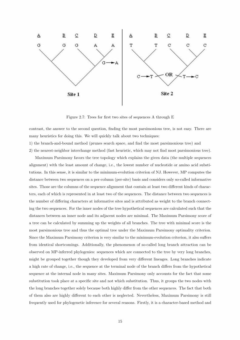
Figure 2.7: Trees for first two sites of sequences A through E

contrast, the answer to the second question, finding the most parsimonious tree, is not easy. There are

many heuristics for doing this. We will quickly talk about two techniques:

1) the branch-and-bound method (prunes search space, and find the most parsimonious tree) and

2) the nearest-neighbor interchange method (fast heuristic, which may not find most parsimonious tree).

Maximum Parsimony favors the tree topology which explains the given data (the multiple sequences

alignment) with the least amount of change, i.e., the lowest number of nucleotide or amino acid substi-

tutions. In this sense, it is similar to the minimum-evolution criterion of NJ. However, MP computes the

distance between two sequences on a per-column (per-site) basis and considers only so-called informative

sites. Those are the columns of the sequence alignment that contain at least two different kinds of charac-

ters, each of which is represented in at least two of the sequences. The distance between two sequences is

the number of differing characters at informative sites and is attributed as weight to the branch connect-

ing the two sequences. For the inner nodes of the tree hypothetical sequences are calculated such that the

distances between an inner node and its adjacent nodes are minimal. The Maximum Parsimony score of

a tree can be calculated by summing up the weights of all branches. The tree with minimal score is the

most parsimonious tree and thus the optimal tree under the Maximum Parsimony optimality criterion.

Since the Maximum Parsimony criterion is very similar to the minimum-evolution criterion, it also suffers

from identical shortcomings. Additionally, the phenomenon of so-called long branch attraction can be

observed on MP-inferred phylogenies: sequences which are connected to the tree by very long branches,

might be grouped together though they developed from very different lineages. Long branches indicate

a high rate of change, i.e., the sequence at the terminal node of the branch differs from the hypothetical

sequence at the internal node in many sites. Maximum Parsimony only accounts for the fact that some

substitution took place at a specific site and not which substitution. Thus, it groups the two nodes with

the long branches together solely because both highly differ from the other sequences. The fact that both

of them also are highly different to each other is neglected. Nevertheless, Maximum Parsimony is still

frequently used for phylogenetic inference for several reasons. Firstly, it is a character-based method and

15

as such considered to be superior to distance methods at it uses all information that is contained in the

input alignment for the tree reconstruction. Secondly, it is fast and therefore an alternative to Maximum

Likelihood for large-scale datasets if computational resources are restricted. Thirdly, the phenomenon of

long-branch attraction is only an issue for small datasets. Fourthly, many biologists appreciate the fact

that MP only makes few assumptions about the evolutionary process besides evolutionary change being

rare.

Branch and bound

The branch-and-bound method (as applied here) counts the number of changes for an initial tree

(e.g., an initial tree may be obtained using the neighbor-joining method). Then, starting from scratch,

we will search our space by building partial trees (i:e:, one branch is added at a time). That is, in the kth

level of the search, we will have nodes representing all possible phylogenetic trees with k leaves for the

first k species (the order is fixed beforehand arbitrarily). If the cost of any partial tree we are building is

greater than that of the initial tree, then search along this line is abandoned. We can improve our search

(potentially getting rid of more things) by computing an estimate of the minimum number of changes

required to add the additional species. There is no guarantee with branch and bound on how much of

the search space is eliminated.

Figure 2.8: Pictorial Example Employing Fitch’s Algorithm for given site

Nearest-neighbor interchange

The nearest-neighbor interchange method involves rearranging trees at the neighbor ” level and

choosing the neighbor” tree with the best score (ie. the least number of changes). There are many

possibilities for how you can define neighbors. Neighbors in this heuristic procedure are defined as

follows. Considering any internal edge, we break up our tree into 4 sub-trees. For example, in the tree

in Figure 4, the subtrees would consist of the leaves A, B, C and D, although in general these subtrees

consist of more than 1 leaf. This original tree (which has A and B branching separately from C and D)

has two neighbors : one with the roles of B and D switched (i.e., with A and D branching separately

from B and C) and one with the roles of B and C switched (i.e., with A and C branching separately

from B and D). Starting with one tree, we repeatedly choose the neighboring tree with the best score,

until there are no neighboring trees with better scores. This is a hill-climbing method, and there is no

guarantee that we will find the most parsimonious tree.

16

While the parsimony method makes very few assumptions, it ignores branch lengths in building trees.

If there are branches that diverge much more rapidly than others, it is easy to convince yourself that the

parsimony method can lead to incorrect topologies.

2.4.3 Maximum Likelihood

Maximum Likelihood is a method for the inference of phylogeny. It evaluates a hypothesis about evolu-

tionary history in terms of the probability that the proposed model and the hypothesized history would

give rise to the observed data set. The supposition is that a history with a higher probability of reaching

the observed state is preferred to a history with a lower probability. The method searches for the tree

with the highest probability or likelihood.

In general, Maximum Likelihood is a parametric statistical method for fitting a mathematical model

to some data. The principle of likelihood suggests that the explanation that makes the observed outcome

the most likely occurrence is the one to be preferred. Formally, given some data D and a hypothesis O,

the likelihood of that data is given by which the probability of obtaining D given v.

L(Dj|O) = f(Dj|O)

Though both terms are colloquially used synonymously, it is important to distinguish between probability

and likelihood here. Informally, probability allows one to predict unknown outcome based on known

parameters, whereas likelihood allows one to predict unknown parameters based on known outcome.

Figure 2.9: Choosing the right algorithm that suits your needs

17

Chapter 3

Data Sets

There are numerous open-source bioinformatics databanks available on internet. Every country is in a

race to develop a rich bioinformatics databank. In this work we select SCBIs DBSNP, EMBL EBIs 1000

genome as a data source from

3.1 The HapMap Project

We have identified one of the sources of data for inferring phylogenetic trees and analyzing them as the

international HapMap project. The International HapMap Project is an effort by multiple countries

to identify and catalog genetic similarities and differences in human beings. Using the information in

the HapMap, researchers will be able to find genes that affect health, disease, and individual responses

to medications and environmental factors. The Project is collaboration among scientists and funding

agencies from Japan, the United Kingdom, Canada, China, Nigeria, and the United States. All of the

information generated by the Project is publically available.

The goal of the International HapMap Project is to compare the genetic sequences of different indi-

viduals to identify chromosomal regions where genetic variants are shared. By making this information

freely available, the Project will help biomedical researchers find genes involved in disease and responses

to therapeutic drugs. In the initial phase of the Project, genetic data are being gathered from four

populations with African, Asian, and European ancestry. Ongoing interactions with members of these

populations are addressing potential ethical issues and providing valuable experience in conducting re-

search with identified populations.

Public and private organizations in six countries are participating in the International HapMap

Project. Data generated by the Project can be downloaded with minimal constraints.

This project is supposed to use the data available at the International Haplotype Map (HapMap Phase

II) for the purpose of conducting a fine-scale genome-wide scan of human genetic variations.Computationally

phased HapMap data is used for this analysis. Although what algorithms we have developed infers max-

imum parsimony phylogenies directly from un-phased data, these algorithms are not efficient enough for

use on a whole-genome scale. We restrict this project to the HapMap population of single subcontinent

because these subpopulations were genotyped for parent-child trios and can thus be expected to have

18

minimal phasing error. The other two HapMap data sets (Han Chinese in Beijing, China and Japanese

in Tokyo, Japan) were genotyped only for unrelated individuals and were omitted here due to the higher

likelihood of phasing errors. All HapMap data sets were downloaded in phased form from the HapMap

web site, where the PHASE program had been used to identify most likely phases from the trio data.

This HapMap build was based on the NCBI human genome assembly build 35. SNP location assign-

ments and genomic coordinates are therefore based on NCBI build 35. The resulting data contained 120

haplotypes from 60 unrelated individuals for each of the two populations typed at approximately 3.7

million SNPs.

Phylogeny inferences are proposed to run for window sizes of five, six, seven, eight, and nine consec-

utive SNPs at each overlapping window of the given size across the 22 autosomal human chromosomes

in each of the HapMap subcontinental populations.

3.2 dbSNP

The Single Nucleotide Polymorphism database (dbSNP) is a database which maintains the variation

(occurring in more than 1

dbSNP is a database that contains entries submitted by public laboratories and private organizations

for a large number of organisms across the globe. Each of these submissions include information about

the actual nucleotide variation and the 5 and 3 flanking sequences.

3.3 The 1000 Genomes Project

The 1000 Genomes Project is the first ever project to sequence the genomes of a large number of people,

to provide a comprehensive data set resource on human genetic variation. The goal of the 1000 Genomes

Project is to locate most genetic variants that have frequencies of at least 1% in the populations under

study. This goal is being attained by sequencing many individuals lightly. To sequence a person’s genome,

many copies of the persons DNA are broken into short pieces and each piece is sequenced individually.

The many copies of DNA indicate that the DNA pieces are more-or-less randomly distributed across the

genome. The pieces are then aligned with the reference sequence and merged together. To accurately

sequence the complete genomic sequence of one person with the existing sequencing platforms, it requires

sequencing that person’s DNA the equivalent of about 28 times. If the amount of sequence done is only

an average of once across the genome, then much of the sequence would be missed, since some genomic

locations will be covered by several pieces while others will have nothing. Deeper the sequencing coverage,

more of the genome will be covered at least once. Also, people are diploid; the deeper the sequencing

coverage, the more likely that both chromosomes at a loci will be included. In addition, deeper coverage

is mainly useful for diagnosing structural variants, and it corrects the sequencing errors.

The 1000 Genome Project offers genome sequences from various families across the geographic loca-

tions. It also maintains the relationship information about the individuals.

19

Chapter 4

Technologies

Following are the technologies we have used in our research.

4.1 Tomcat Server

We use Tomcat Server to provide web based access to our system. Also the comcat server is used to deploy

the webservice clients for the Multiple Sequence alignment through Clustal Omega and Phylogenetic

Trees through Clustal Phylogeny from EMBL EBI.

4.2 Web Services

Web services are application components providing access to certain methods and objects through in-

ternet. Web services communicate using open protocols like tcp/ip and http and make it easy to access

the components across the platforms. Web services are self contained and self describing services. All

this description is offered through an XML file with extension as wsdl (stands for web service description

language). Web services are discovered using UDDI (Universal Description Discovery and Integration)

which allows the client to connect with a specific web service running on that server. Web services can

also be used by other applications existing within the local area network of the server or through inter-

net. XML is the base for Web services as it offers interoperability across the platforms and simplifies the

communication through basic protocols.

The basic Web services platform is XML and HTTP protocol combination. XML offers a language

which can be used across different platforms and programming languages and still deliver complex mes-

sages and functions. The HTTP protocol is the core and most used Internet protocol. Web services

platform elements include:

• SOAP - (Simple Object Access Protocol)

• UDDI - (Universal Description, Discovery and Integration)

• WSDL - (Web Services Description Language)

20

Various web service are offered by the global bioinformatics community. And we have used a couple

of them offered by EMBL EBI. The web services that we have used are ClustalOmega for Multiple

Sequence Alignment And ClustalW2 Phylogeny for retrieving phylogenetic tree related data.

4.3 JSP (Java Server Pages)

Java Server Pages (JSP) is a technology for developing dynamic web pages that is to provide support

dynamic content. It helps developers insert java code in HTML pages by making use of special JSP

tags. A JSP component is a type of Java servlets that is designed to interact with the client offering

realtime contents using a Java web application. The JSP files are written as text files that combine

HTML or XHTML code, XML elements, and embedded JSP actions and commands in order to offer

dynamic contents. The User interface for JSP is offered through web browsers as JSP happens to be a

web application development language.

JavaServer Pages often offers the same applications as offered by Common Gateway Interface (CGI)

language but on the top of it has tons of benefits both functional and non functional. Performance is

significantly improved because JSP allows embedding Dynamic Elements in HTML Pages itself instead of

having a separate CGI files. JSP files are always compiled before it’s processed by the server as opposed

to CGI/Perl which requires the server to load an interpreter and the target script each time the page is

requested. JavaServer Pages are built using the base as the Java Servlets API, so like Servlets, JSP also

has access to all the powerful Enterprise Java APIs, including JDBC, EJB, JNDI, JAXP etc. JSP pages

can also be used in combination with servlets that are used to handle the business logic, the model that

is supported by Java servlet template engines. JSP is an integral part of J2EE, a complete platform for

enterprise standard applications. This implies that JSP can be used to develop simplest applications to

the most complex and demanding applications.

4.4 HTML 5

HTML5 is a co-operation between the (W3C) World Wide Web Consortium and the (WHATWG) Web

Hypertext Application Technology Working Group. HTML5 is the new standard for HTML. For HTML5

still a lot of work is in progress. However, Many browsers have incorporated support for HTML 5. It

heavily uses java script and CSS. By use of these technologies it reduces the use of external plugins like

flash, reduces use of scripting by incorporating new tags, and has improved on error handling. Also

HTML5 targets to be compatible with every device. In our research we have used the canvas tag in

combination with the java scrip language for rendering the results in the form of phylogenetic trees.

4.5 Java Script

A scripting language is a lightweight programming language used with the web applications. This is

client side scripting language mainly used for data validation, animations, and small calculations at the

21

client end. It is programming code that can be inserted into HTML pages. JavaScript when inserted

into HTML pages, is supported by all modern web browsers and hence can be executed with ease. It

can detect the browser the client is using so that respective code can be executed. The java script is an

interpreted language that is you do not need to compile it before execution, its directly interpreted by

the web browser.

4.6 Eclipse

Eclipse is an opensource IDE Integerated Development Environment. It is created by Open Source

Community and is used in several different areas, e.g. as a development environment for Java or Android

applications, python, c, c++ pearl etc. The Eclipse projects are governed by the Eclipse Foundation. The

Eclipse Foundation is a member supported, non-profit corporation that hosts the Eclipse Open Source

projects. Also helps to cultivate both an Open Source community and an Ecosystem of complementary

products and services. The Eclipse IDE can be easily extended with additional software components or

plugins. Several Open Source projects and companies have extended the Eclipse IDE and customized

according to their requirements in their working environment.

Eclipse is also used as a base for creating general purpose applications. These applications are known

as Eclipse Rich Client Platform applications (Eclipse RCP). The Eclipse Foundation uses Eclipse Public

License (EPL) and is an Open Source software license for its software. The EPL is specially designed to

be business-friendly. EPL Licence states that the EPL licensed programs can be used, modified, copied

and distributed free of cost. The consumer of EPL licensed software can go for using this software in

closed source programs. Any modifications in the original EPL code must also be released as EPL code

as stated by EPL.

We have extensively used Eclipse IDE for implementing our algorithm by implementing the web

service clients and our intermediate code and the HTML 5 with Java Script code.

22

Chapter 5

DiagnosTree -The Tool

We name our tool as DiagnosTree since it facilitates diagnosis of diseases through the use of phylogenetic

trees.

Although the diagnosis is possible with gene sequences, protein sequences, and the RNA sequences,

but for this paper we will stick to gene sequences. Our method is based on the similarity that the human

beings are having in their gene sequences and the assumption that any change in the gene sequence at

the loci where the nitrogen bases are usually common in all the human beings is responsible for the

abnormality an individual is having.

5.1 The Algorithm

5.1.1 Required Inputs

• Patients gene sequence

• A few of Patients family members gene sequences

• Diseased gene sequences (which will be downloaded from the Bioinformatics databases).

We consider patients family members sequences for analysis since their gene sequences are most close

to the patients gene sequence, with the help of these sequences we try to find out which mutation in the

sequence of the patient is responsible for the disorder. To diagnose the disease we need to compare the

sequence of the patient with the gene sequences of diseased genomes. To reduce the time required for

diagnosis (through computer processing) we suggest to find out the probable diseases the patient might

be suffering from based on the symptoms. In our method we find out the common nucleotides among

the patient and the family members gene sequences and discard the dissimilar nucleotides to retain the

common nucleotides with respect to their loci. Following are the steps that we suggest to diagnose the

disease.

Step 1: Align the gene sequences of

• The patient

23

• The family members of the patient

• And the diseased sequences.

Step 2: Find out the common nucleotides among the family members of the patient, and discard the

dissimilar nucleotides from all the sequences (of the patient, patients family members, and the diseased

sequences) from the respective loci after alignment.

Step 3: Now Discard the Patients family members gene sequences.

Step 4: Create a phlyogenetic tree (we prefer maximum parsimony based phylogenetic tree) based

on the sequences we got in the previous step (Modified gene sequences of the patient and the diseased

sequences).

Step 5: From this tree we can say that the patient is suffering from a disease which is having least

distance from the patients gene sequence.

5.1.2 Example

Lets consider the following hypothetical sequences.

Figure 5.1: Set of Input Sequences

Where P is the Patient, F1, F2, F3 and F4 are close relatives of the patient and D1, D2, D3 and D4

are People suffering from different diseases (Reference sequences).

Now we do apply multiple sequence alignment on these sequences and get the following output.

From the above result we discard the dissimilar nucleotides/characters from the family members

sequences and discard the nucleotides/characters at respective loci from the other sequences as follows.

And we get

Further we ignore the close relatives sequences and construct a phylogenetic tree based on the rest of

the sequences.

The tree shown in the above figure depicts that the patient is suffering from the disease D2.

24

Figure 5.2: Aligned Sequences (Output of MSA)

Figure 5.3: Uncommon Nucleotieds to be omitted out of the sequences

25

Figure 5.4: Set of Family Members Sequences to be removed from The Sequences

Figure 5.5: Final set of Sequences to be used for creating The Phylogenetic Tree

Figure 5.6: The resultant Tree depicting relationship among the patients gene sequence and different

diseased sequences

26

Chapter 6

System Architecture

Figure 6.1: Layered System Architecture

27

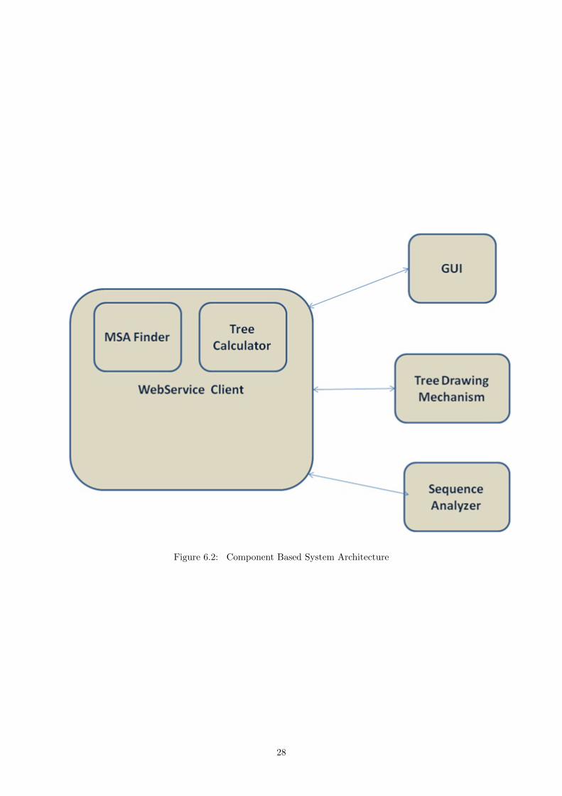
Figure 6.2: Component Based System Architecture

28

Figure 6.3: Flowchart for the Algorithm29

Chapter 7

Results

After using the sequences from 1000 genome project, dbSNP and HapMap databases we got accurate

results the algorithm . We have used the family memeber’s sequences from the 1000 genome project

and the reference disease sequences from dbSNP. After doing 30 such tests on the algorithm we found

that our algorithm gave all the results as correct. The only concern remains here is the set of Diseased

sequences. As of now there are thousands of diseases. And if the sequences are not opt properly there is

a danger of mis-diagnosis. To avoid this scenario we need to use the sequences of all the existing diseases

which incurr a lot of computational resourcers and is very time consuming, that is it may take months of

time to give the result. We have an agenda of working out on this scenario and sort out an optimmum

resultant algorithm.

Half the portion of the algorithm in our tool is executed on the other servers the portion of code

which excutes at the local system is very efiicient and has proved to take O(n2) time. The tool requires

a cluster of workstations if needed to execute the entire algorithm on the local system. Such a use and

analysis is out of the scope of this project thesis as of now.

Following are few input sequences on which we have tested the algorthm:

• Family ID:13291 Individual ID:NA06986

• Family ID:13291 Individual ID:NA06995

• Family ID:13291 Individual ID:NA06997

• Family ID:13291 Individual ID:NA07037

• Family ID:13291 Individual ID:NA07045

• Family ID:13291 Individual ID:NA07435

The result after aplication of our algorithm happens to be the individual ”NA07435” is suffering from

Alzhymers and is as provided with the database itself.

30

Chapter 8

Conclusion

The phylogenetic trees are beinng utilized to diagnose the disease after multiple sequence analysis on

the various sequences. This improves the diagnosis process and hence accelerating the process of treat-

ment. The open source bioinformatics resources should be utilized to improve the Disease Diagnosis and

Treatment process such that the current loop holes in the medical system must be closed and human

society must be benefited. To this end we present a novel algorithm which makes an effort to effectively

utilize the available bioinformatics services and databases to enhance the accuracy and performance of

diagnosis process. We believe that our work can be used to improve the current scenario in the medical

system and benefit the society to become more secure against the diseases. Since diagnosis of a disease

is half the recovery.

31

Chapter 9

Future Work

We believe that there is a scope to further improve the proposed algorithm so as to target the non-

genetic diseases which have an impact over the genome sequences. Also there is a scope to improve the

performance of this Algorithm by parallelizing it and improve the comparison methods used here. We

plan to implement our own service as an open application available in public, so that the research process

in this direction can be improved.

32