Using Multilevel Modeling to Analyze Longitudinal DataMark A. Ferro, PhDOfford Centre for Child Studies Lunch & Learn Seminar SeriesJanuary 22, 2013

Recommended Readings1. Singer JD, Willett JB. Applied longitudinal data analysis. Modeling

change and event occurrence. New York: Oxford University Press; 2003.

2. Singer JD. Fitting individual growth models using SAS PROC MIXED. In: Moskowitz DS, Hershberger SL, editors. Modeling intraindividual variability with repeated measures data. Methods and applications. Mahwah: Lawrence Erlbaum Associates; 2002.

3. Singer JD. Using SAS PROC MIXED to fit multilevel models, hierarchical models, and individual growth models. J Educ Behav Stat 1998;24: 323-55.

Objectives

1. Explore longitudinal dataa) Wrong approaches

2. Understand multilevel model for changea) Specify the level-1 and level-2 modelsb) Interpret estimated fixed effects and variance components

3. Data analysis with the multilevel modela) Adding level-2 predictorsb) Comparing models

Research Questions• Broadly speaking, we are interested in two types of questions:

1. Start by asking about systematic change over time for each individual

2. Next ask questions about variability in patterns of change over time (what factors may help us explain different patterns of growth?)

Wrong Approaches1. Estimated correlation

coefficients:• Problem: only measures

status, not change (tells whether rank order is similar at both time-points)

2. Use difference score to measure change and use this as an estimate of rate of change• Problem: assumes linear

growth over time, but change may be non-linear

25 50 75 1000

255075

100

Grade 8

Gra

de 9

6 7 8 9 10 110

25

50

75

Grade

Mat

h Sc

ore

Less-than-Ideal Approaches

1. Aggregate data• Reduced power• No intra-individual

variation

2. Repeated Measures ANOVA• Reduced power• Equal linear change• Compound symmetry

Class 1

Patient 1

Time 1

Time 2

Time 3

Patient 2

Time 1

Time 2

Time 3

Class 2

Patient 3

Time 1

Time 2

Time 3

Patient 4

Time 1

Time 2

Time 3

Level 2

Level 1

Class 2

Patient 3

Time 1

Time 2

Patient 4

Time 1

Time 2

Time 3

Level 2

Level 1

Class 1

Patient 1

Time 1

Time 2

Time 3

Patient 2

Time 1

Time 2

0

2

8

0

1

2

Advantages of MLM• Flexibility in research design• Different data collection schedules• Varying number of waves

• Identify temporal patterns in the data

• Inclusion of time-varying predictors

• Interactions with time• Effects that get smaller or larger over time

Example Dataset• Longitudinal Study of American Youth (LSAY)• N=1322 Caucasian and African-American students• Change in mathematics achievement between grades 7-11

1. At what rate does mathematics achievement increase over time?

2. Is the rate of increase related to student race, controlling for the effects of SES and gender?

How to Answer the Questions?

1. Exploratory analysis2. Fit taxonomy of progressively more complex models

a) Unconditional means model (not shown)b) Unconditional linear growth modelc) Add race as level-2 predictor of initial status and rate of change

in match achievementd) Add SES as level-2 control variable, testing impact on initial

status and rate (does effect of race change?)e) Add gender as level-2 control variable,…

3. Select final model and plot prototypical trajectories4. Residual analysis to evaluate tenability of assumptions

Multilevel Model for Change• Level-1 model:

• Level-2 model:

• Composite model:

structural stochastic

ijijiiij tY 10

iii

iii

race

race

111101

001000

)(

)(

ijijiiijiiijij ttraceracetY 1001011000

Level-1 Model• Within-individual

• Intercept of individual i’s trajectory (initial status)• Centred at a time 0• Math achievement at time 0

• Slope of individual i’s trajectory (rate of change)• Change in math achievement between each time point

• Deviations of individual i’s trajectory from linearity on occasion j (error term)

• ~N(0,σ2)

ijijiiij tY 10

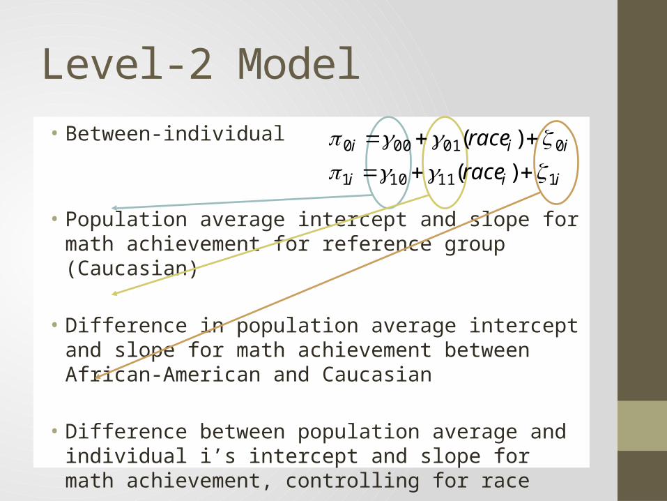
Level-2 Model• Between-individual

• Population average intercept and slope for math achievement for reference group (Caucasian)

• Difference in population average intercept and slope for math achievement between African-American and Caucasian

• Difference between population average and individual i’s intercept and slope for math achievement, controlling for race

iii

iii

race

race

111101

001000

)(

)(

Level-2 Model Residuals• Variance-covariance matrix

• Population variance in intercept, controlling for race

• Population variance in slope, controlling for race

• Population covariance between intercept and slope, controlling for race

2110

0120

1

0 ,0

0~

Ni

i

Exploratory Analysis - OLS

SAS Syntaxproc mixed data=lsay noclprint noinfo covtest method=ml;title 'Model A: Unconditional Linear Growth Model';class lsayid;model math = grade_c / solution ddfm=bw notest;random intercept grade_c /subject=lsayid type=un;run;

Unconditional Linear Growth – Fixed Effects

Solution for Fixed EffectsEffect Estimate Standard

ErrorDF t Value Pr > |t|

Intercept 52.3660 0.2541 1321 206.10 <.0001grade_c 2.8158 0.0732 5102 38.46 <.0001

00

Estimated math achievement in 7th grade

10

Estimated yearly rate of change in math achievement

t-test for null H0 of no average change in achievement in the population

Unconditional Linear Growth – Random Effects

Covariance Parameter EstimatesCov Parm Subject Estimate Standard

ErrorZ Value Pr Z

UN(1,1) LSAYID 62.4944 3.3638 18.58 <.0001UN(2,1) LSAYID 6.4550 0.7011 9.21 <.0001UN(2,2) LSAYID 3.2164 0.2906 11.07 <.0001Residual   37.1645 0.8552 43.46 <.0001

20

Estimated variance in intercept

21

Estimated variance in slope

2

Estimated variance in level-1 residuals

01Estimated covariance between intercept and slope

SAS Syntaxproc mixed data=lsay noclprint noinfo covtest method=ml;title 'Model B: Adding the Effect of Race';class lsayid;model math = grade_c aa aa*grade_c / solution ddfm=bw notest;random intercept grade_c /subject=lsayid type=un;run;

Adding the Effect of Race – Fixed Effects

Solution for Fixed EffectsEffect Estimate SE DF t Value Pr > |t|Intercept 53.0170 0.2638 1320 201.00 <.0001grade_c 2.8688 0.0775 5101 37.03 <.0001aa -5.9336 0.7969 1320 -7.45 <.0001grade_c*aa -0.4822 0.2341 5101 -2.06 0.0395

00Estimated math achievement in 7th grade for Caucasians

10 Estimated yearly rate of change in math achievement for Caucasians

11 Estimated difference in yearly rate of change in math achievement between Caucasian and AA

01Estimated difference in math achievement in 7th grade between Caucasians and AA

Adding the Effects of Race – Random Effects

Covariance Parameter EstimatesCov Parm Subject Estimate SE Z Value Pr ZUN(1,1) LSAYID 59.0450 3.2313 18.27 <.0001UN(2,1) LSAYID 6.1765 0.6868 8.99 <.0001UN(2,2) LSAYID 3.1930 0.2899 11.01 <.0001Residual   37.1671 0.8553 43.46 <.0001

20

Estimated variance in intercept, controlling for race21

Estimated variance in slope, controlling for race

2

Estimated variance in level-1 residuals

01Estimated covariance between intercept and slope, controlling for race

SAS Syntaxproc mixed data=lsay noclprint noinfo covtest method=ml;title 'Model B: Adding the Effect of Race';class lsayid;model math = grade_c aa aa*grade_c ses ses*grade_c / solution ddfm=bw notest;random intercept grade_c /subject=lsayid type=un;run;

Adding the Effects of SES – Fixed Effects

Effect Estimate SE DF t Value Pr > |t|Intercept 52.8064 0.2537 1319 208.13 <.0001grade_c 2.8462 0.0774 5100 36.79 <.0001aa -4.6620 0.7734 1319 -6.03 <.0001ses 3.6210 0.3379 1319 10.72 <.0001grade_c*aa -0.3491 0.2358 5100 -1.48 0.1389grade_c*ses 0.3718 0.1029 5100 3.61 0.0003

00Estimated math achievement in 7th grade for Caucasians of average SES

10 Estimated yearly rate of change in math achievement for Caucasians of average SES

11 Estimated difference in yearly rate of change in math achievement between Caucasian and AA, controlling for SES

01Estimated difference in math achievement in 7th grade between Caucasians and AA, controlling for SES

02Estimated effect of SES on average 7th grade achievement, controlling for race

02 Estimated effect of SES on rate of change of achievement, controlling for race

Adding the Effects of SES – Random EffectsCov Parm Subject Estimate Standard

ErrorZ Value Pr Z

UN(1,1) LSAYID 52.4635 2.9794 17.61 <.0001UN(2,1) LSAYID 5.5022 0.6587 8.35 <.0001UN(2,2) LSAYID 3.1260 0.2874 10.88 <.0001Residual   37.1684 0.8553 43.46 <.0001

20

Estimated variance in intercept, controlling for race and SES21

Estimated variance in slope, controlling for race and SES

2

Estimated variance in level-1 residuals

01Estimated covariance between intercept and slope, controlling for race and SES

SAS Syntaxproc mixed data=lsay noclprint noinfo covtest method=ml;title 'Model B: Adding the Effect of Race';class lsayid;model math = grade_c aa aa*grade_c ses ses*grade_c / solution ddfm=bw notest;random intercept grade_c /subject=lsayid type=un;run;

Removing the Effect of Race on Rate of Change

Solution for Fixed EffectsEffect Estimate Standard

ErrorDF t Value Pr > |t|

Intercept 52.8183 0.2536 1319 208.28 <.0001grade_c 2.8074 0.0729 5101 38.53 <.0001aa -4.7698 0.7700 1319 -6.19 <.0001ses 3.6139 0.3379 1319 10.70 <.0001grade_c*ses 0.3954 0.1018 5101 3.89 0.0001

SAS Syntaxproc mixed data=lsay noclprint noinfo covtest method=ml;title 'Model B: Adding the Effect of Race';class lsayid;model math = grade_c aa ses ses*grade_c female / solution ddfm=bw notest;random intercept grade_c /subject=lsayid type=un;run;

Final Model with GenderSolution for Fixed EffectsEffect Estimate Standard

ErrorDF t Value Pr > |t|

Intercept 52.4013 0.3504 1318 149.55 <.0001grade_c 2.8077 0.0729 5101 38.53 <.0001aa -4.7982 0.7693 1318 -6.24 <.0001ses 3.6159 0.3375 1318 10.71 <.0001female 0.8183 0.4751 1318 1.72 0.0852grade_c*ses 0.3953 0.1017 5101 3.89 0.0001

Goodness-of-FitModel A Model B Model C Model D Model E Model F

Deviance 45443.4 45383.0 45253.2 45255.4 45252.2 45252.4

AIC 45455.4 45399.0 45723.2 45273.2 45274.2 45272.4

BIC 45486.5 45440.5 45325.1 45320.1 45331.2 45324.3

Deviance• -2LL statistic• Worse fit = larger -2LL• Can be compared in nested models• χ2 distribution, df = difference in number of parameters

AIC & BIC• Can be used for non-nested models• AIC corrects for number of parameters estimated• BIC corrects for sample size and number of parameters, so larger

improvement needed for larger samples

Presenting Results

Ferro & Boyle. Journal of Pediatric Psychology 2013;38(4):425-37

Plotting Trajectories for Prototypical Individuals

Race SES Initial Status Rate of Change

Caucasian Low 52.401-4.798(0)+3.616(-0.693)+0.818(1)=50.713 2.808+0.395(-0.693)=2.534

Caucasian High 52.401-4.798(0)+3.616(0.735)+0.818(1)=55.877 2.808+0.395(0.735)=3.098

AA Low 52.401-4.798(1)+3.616(-0.693)+0.818(1)=45.915 2.808+0.395(-0.693)=2.534

AA High 52.401-4.798(1)+3.616(0.735)+0.818(1)=51.079 2.808+0.395(0.735)=3.098

Estimates of initial status and rate of change for Caucasian and African-American girls of high and low SES

Prototypical Trajectories

7 8 9 10 1140

45

50

55

60

65

70

Caucasian, High SESAA, High SESCaucasian, Low SESAA, Low SES

Grade

Estim

ated

Mat

h A

chie

vem

ent

Assumptions & Evaluation

Assumption

1. Level-1 growth model is linear

2. Level-2, relationship between predictors and intercept and slope is linear

3. Level-1 and level-2 residuals are normal and homoscedastic

Evaluation

1. Examine empirical growth plots for evidence of linearity

2. Plot OLS estimates of growth parameters vs. each predictor

3. Standard diagnostics for level-1 and level-2