Using Microsoft Excel Microsoft Excel 7... · 2018-04-14 · Using Microsoft Excel Advanced Skills...
24
Using Microsoft Excel 2016 Advanced Skills © Steve O’Neil 2018 Page 1 of 24 http://www.oneil.com.au/pc/ Using Microsoft Excel Advanced Skills Excel contains numerous tools that are intended to meet a wide range of requirements. Some of the more specialised tools are useful to people in certain situations while others have value for more general excel users. These exercises will cover some of the advanced features that may be useful for most excel users. These features will include cell naming, cell notes, conditional formatting, data validation and custom number formats. Naming Cells In a large spreadsheet, cell referencing and selection may be simplified by making use of names. You can assign a unique name to an individual cell or to a range of cells. This can make it quicker and easier to refer to the cells in charts and functions. Additionally, functions that make use of names are easier to read. For instance, a formula that says =B4-B5 isn’t as clear as a formula that says =Sales-Expenses. Exercise 1. Creating Cell Names 1) Create a new workbook in Excel and create a table like the one below.
Transcript of Using Microsoft Excel Microsoft Excel 7... · 2018-04-14 · Using Microsoft Excel Advanced Skills...
Using Microsoft Excel 2016 Advanced Skills
© Steve O’Neil 2018 Page 1 of 24 http://www.oneil.com.au/pc/
Using Microsoft Excel
Advanced Skills
Excel contains numerous tools that are intended to meet a wide
range of requirements. Some of the more specialised tools are
useful to people in certain situations while others have value for
more general excel users. These exercises will cover some of the
advanced features that may be useful for most excel users. These
features will include cell naming, cell notes, conditional
formatting, data validation and custom number formats.
Naming Cells
In a large spreadsheet, cell referencing and selection may be simplified by making use
of names. You can assign a unique name to an individual cell or to a range of cells.
This can make it quicker and easier to refer to the cells in charts and functions.
Additionally, functions that make use of names are easier to read. For instance, a
formula that says =B4-B5 isn’t as clear as a formula that says =Sales-Expenses.
Exercise 1. Creating Cell Names
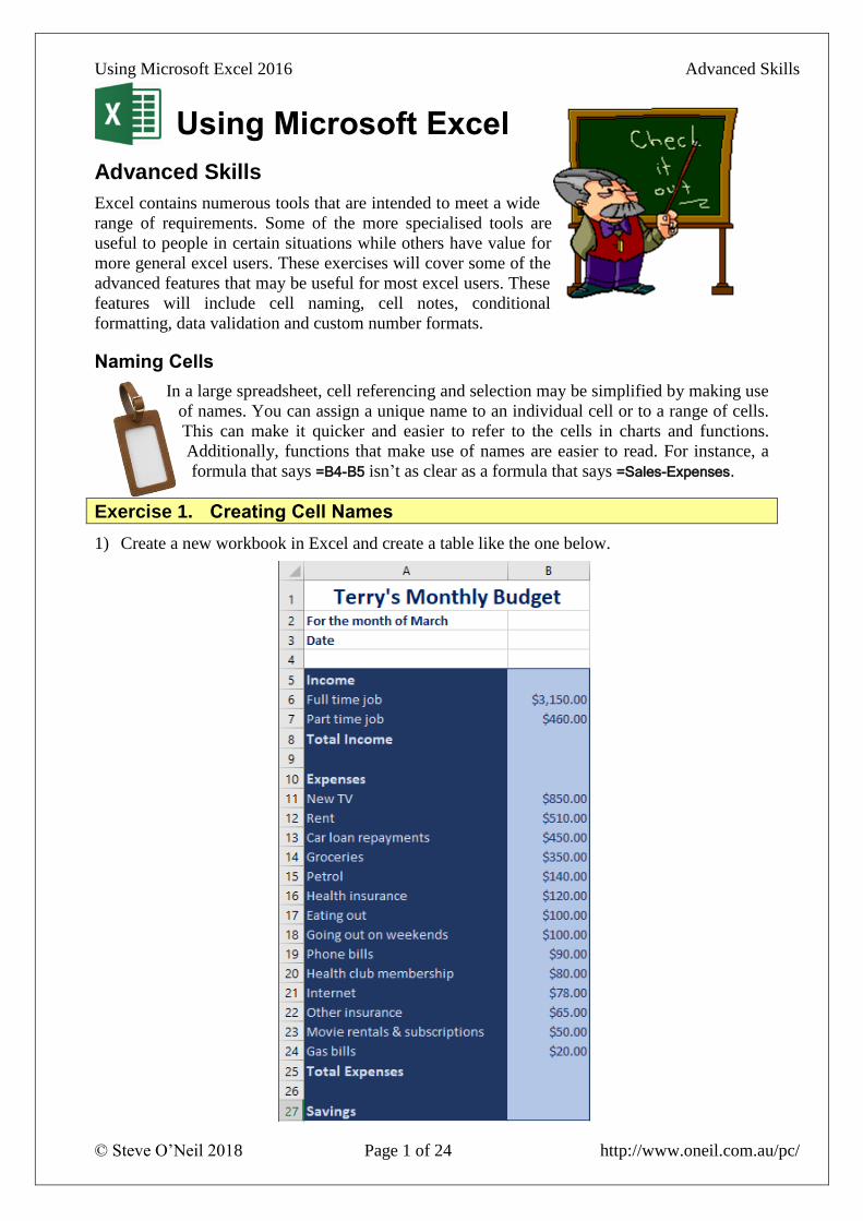
1) Create a new workbook in Excel and create a table like the one below.

Using Microsoft Excel 2016 Advanced Skills
© Steve O’Neil 2018 Page 2 of 24 http://www.oneil.com.au/pc/
2) Save the file as Budget.
3) Click on Cell A3 which will have the current date.
4) Click in the Names box which is to the left of the formula bar. Currently it will display the
reference of the currently selected cell.
5) Type Date in the box and press [Enter] to create the name for that cell.
6) Click in another cell anywhere on the worksheet (or even in another worksheet).
7) Click on the dropdown arrow next to the Names box. A list of names for the current
workbook will appear.
8) Click on the Date name. Excel will automatically go to, and select that named cell, even if
you were on a different sheet.
Note Whenever you select a cell or range of cells that is named, the name will appear in the names box instead of the cell reference.
9) Select the cell range B6:B7 which should contain the cells with the income amounts.
10) Click in the Names box, type Income and press [Enter].
Note If you type a name in the names box without pressing [Enter] afterwards, the name might not be created.
11) Select the cell range B11:B24 which should contain the expense figures.
12) Click in the Names box, type Expenses and press [Enter].
13) Test the new named ranges by selecting them from the names dropdown
list. Each range should become selected when you select its range.
14) Click in cell D8. This cell will contain the formula to calculate total income.
15) Enter the following formula.
=Sum(Income)
Excel will make use of the range name to add up all of the cells in that range.
16) Click in cell B26 which will contain the total expenses.
17) Click on the Autosum icon.
When the Autosum tool completes the function, it will
use the range name you have created instead of the less
meaningful cell references.
18) Press [Enter] to complete the function.
19) Save the changes to the workbook.

Using Microsoft Excel 2016 Advanced Skills
© Steve O’Neil 2018 Page 3 of 24 http://www.oneil.com.au/pc/
Exercise 2. Creating Names Automatically
If you have a lot of cells you want to name, it is possible to have the names automatically
created for you from table headings/labels.
1) Select A6:B8. These cells contain the income labels and amounts.
2) From the Formulas tab on the Ribbon click the Create from
Selection icon.
3) We want the data cells to be named based on the cells in the left column so make sure the
Left column option is selected and then click OK.
4) Click in cell B6, B7 or B8. Look in the Names box to see the names that have been created.
Notice that names with more than one word have been created using an underscore. E.g. cell
B8 will now have the name Total_Income. This is
because names cannot contain spaces. Names must
also begin with a letter.
Tip If there isn’t enough room to show the whole name, you can resize the cell name area by dragging the small dotted symbol between the names box and the formula bar.
5) Select the cell range A11:B25. This should contain the expenses data and labels.
6) Click .
7) Click OK to define names for these cells.
We can view, modify or delete the names that have already been created by using the Name
Manager options.

Using Microsoft Excel 2016 Advanced Skills
© Steve O’Neil 2018 Page 4 of 24 http://www.oneil.com.au/pc/
8) Make sure the Formulas tab is still selected and click the Name Manager icon.
This dialog lists all the names in the current workbook. From here you can delete names and
modify the cells that a name refers to.
9) Scroll through the list to see information about each of the names.
10) Click Close to close the dialog without making any changes.

Using Microsoft Excel 2016 Advanced Skills
© Steve O’Neil 2018 Page 5 of 24 http://www.oneil.com.au/pc/
Exercise 3. Pasting Names
When you are creating a formula you can use names as you
have already seen. If your workbook has a lot of names,
however, then it may be difficult to type a particular name
from memory. You can’t select names from the names box
since when you are editing a formula; the names box changes
in to a list of commonly used functions as shown to the right.
Instead you can insert a name in to a formula.
1) Click in cell B28. This is where we will calculate the savings in the budget.
2) Type an equals sign = to begin a formula.
3) From the Formulas tab click . Notice that many of the other ribbon options
are not available while you are editing a cell. A list of names you can use in your formula
will appear.
4) From the list select Total_Income. The name will be inserted in to the formula.
5) Type a minus sign. –
6) Click .
7) Select Total_Expenses from the list and click OK.
The formula should appear as
8) Press [Enter] to complete the formula.
Note When you are editing a formula, a list of names and functions will appear next to where you are typing. You can double-click from the list as you type to insert them in to your formula.
Using Microsoft Excel 2016 Advanced Skills
© Steve O’Neil 2018 Page 6 of 24 http://www.oneil.com.au/pc/
Cell Comments
Cell comments can be used to provide handy information to a person who is using your
spreadsheet. They can contain tips, and other information that may be helpful. They are
indicated by a small red triangle in the corner of the cell. When the mouse is moved over the
cell, the note will appear for the user. Comments can be formatted to match the look of the rest
of the spreadsheet.
Exercise 4. Creating a Cell Comment
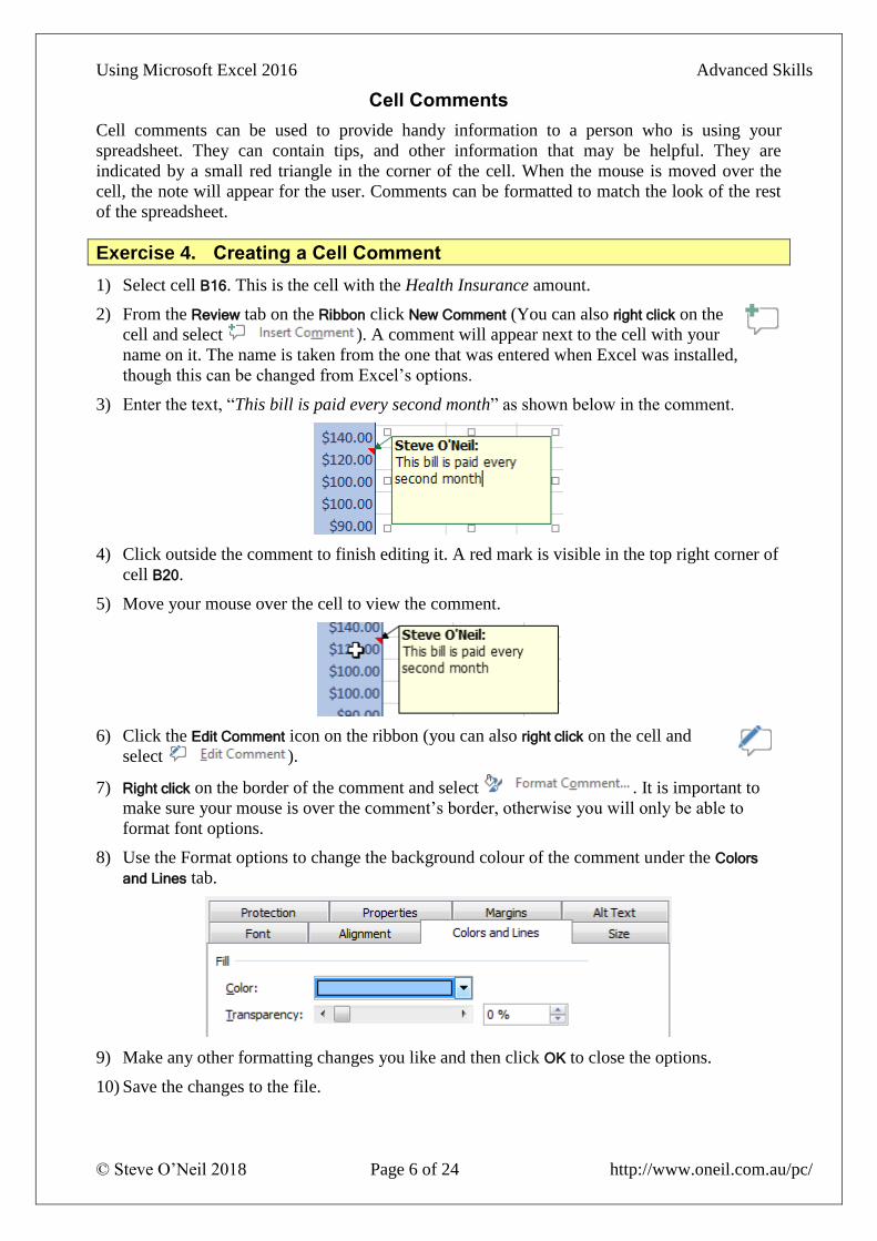
1) Select cell B16. This is the cell with the Health Insurance amount.
2) From the Review tab on the Ribbon click New Comment (You can also right click on the
cell and select ). A comment will appear next to the cell with your
name on it. The name is taken from the one that was entered when Excel was installed,
though this can be changed from Excel’s options.
3) Enter the text, “This bill is paid every second month” as shown below in the comment.
4) Click outside the comment to finish editing it. A red mark is visible in the top right corner of
cell B20.
5) Move your mouse over the cell to view the comment.
6) Click the Edit Comment icon on the ribbon (you can also right click on the cell and
select ).
7) Right click on the border of the comment and select . It is important to
make sure your mouse is over the comment’s border, otherwise you will only be able to
format font options.
8) Use the Format options to change the background colour of the comment under the Colors
and Lines tab.
9) Make any other formatting changes you like and then click OK to close the options.
10) Save the changes to the file.
Using Microsoft Excel 2016 Advanced Skills
© Steve O’Neil 2018 Page 7 of 24 http://www.oneil.com.au/pc/
11) Click the File tab on the Ribbon and then click Print.
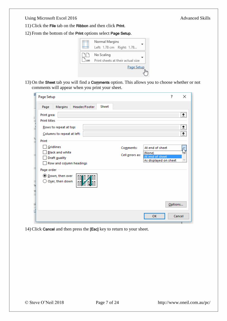
12) From the bottom of the Print options select Page Setup.
13) On the Sheet tab you will find a Comments option. This allows you to choose whether or not
comments will appear when you print your sheet.
14) Click Cancel and then press the [Esc] key to return to your sheet.

Using Microsoft Excel 2016 Advanced Skills
© Steve O’Neil 2018 Page 8 of 24 http://www.oneil.com.au/pc/
Conditional Formatting
Conditional formatting allows you to create rules that will change the formatting in a cell based
on the values in the cell. It can be useful for highlighting certain parts of the spreadsheet when
certain conditions are met. In our table we will apply conditional formatting to highlight
different expenses.
Exercise 5. Applying Conditional Formatting
1) From the Names drop down list, select Expenses. All of the expenses cells should be
selected.
2) Make sure the Home tab is selected and click Conditional Formatting.
First we’ll test out some of the Bars, scales and icon sets.
3) Select the Data Bars option from the list.
4) Move your mouse over some of the data bar options and your spreadsheet will show a
preview of how that option looks.
5) Select the Color Scales option.
6) Move your mouse over some of the colour scales options to see how they would look.
7) Select the Icon Sets option.
8) Move your mouse over some of the icon sets options to see how they would look.
Using Microsoft Excel 2016 Advanced Skills
© Steve O’Neil 2018 Page 9 of 24 http://www.oneil.com.au/pc/
In addition to the built in conditional format sets, you can create your own conditional format
rules.
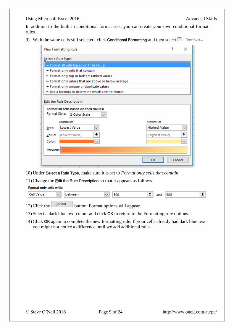
9) With the same cells still selected, click Conditional Formatting and then select
10) Under Select a Rule Type, make sure it is set to Format only cells that contain.
11) Change the Edit the Rule Description so that it appears as follows.
12) Click the button. Format options will appear.
13) Select a dark blue text colour and click OK to return to the Formatting rule options.
14) Click OK again to complete the new formatting rule. If your cells already had dark blue text
you might not notice a difference until we add additional rules.
Using Microsoft Excel 2016 Advanced Skills
© Steve O’Neil 2018 Page 10 of 24 http://www.oneil.com.au/pc/
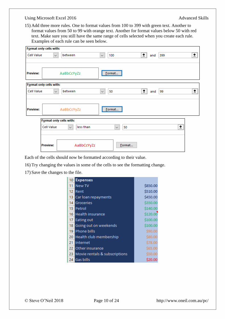
15) Add three more rules. One to format values from 100 to 399 with green text. Another to
format values from 50 to 99 with orange text. Another for format values below 50 with red
text. Make sure you still have the same range of cells selected when you create each rule.
Examples of each rule can be seen below.
Each of the cells should now be formatted according to their value.
16) Try changing the values in some of the cells to see the formatting change.
17) Save the changes to the file.

Using Microsoft Excel 2016 Advanced Skills
© Steve O’Neil 2018 Page 11 of 24 http://www.oneil.com.au/pc/
Exercise 6. Printing Options
1) Select the File tab on the Ribbon and then select Print (or press [Ctrl] [P] ). Options like the
ones below will appear. The right section shows a preview of what your page will look like
when printed with the selected options. If your sheet covers more than one page, you can use
the buttons at the bottom to select which page is showing in the preview.
2) To print with the standard options, select the number of copies required and then click the
Print button as shown below.
The next option shows the currently selected printer. If you click on it you can select from a list
of the printers that are available on your computer. Many of the following options will depend
on the printer that is selected. For instance, not all printers are capable of double sided printing.
3) Select one of the printers in the list and then click Printer Properties. This will display some of
the options that are specific to the selected printer. These often include options for print
quality and paper types.
Using Microsoft Excel 2016 Advanced Skills
© Steve O’Neil 2018 Page 12 of 24 http://www.oneil.com.au/pc/
4) Click Cancel to close the Printer Properties and return to Excel’s print options.
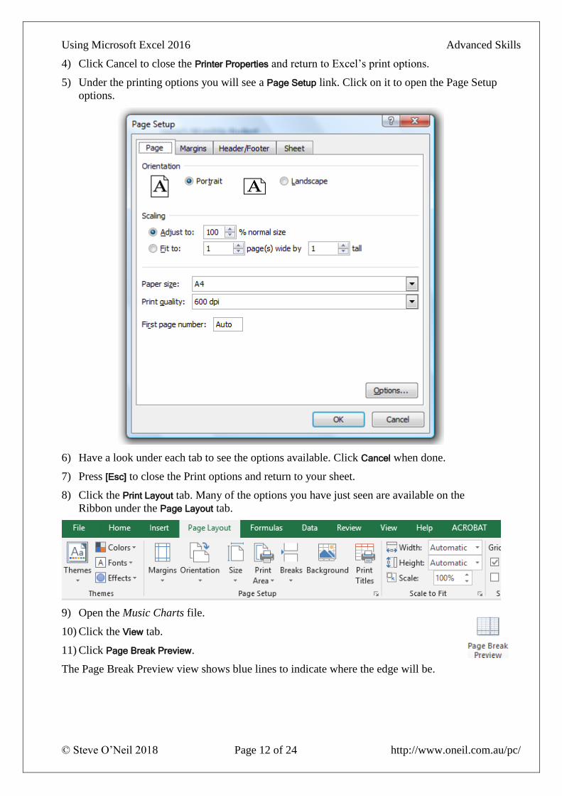
5) Under the printing options you will see a Page Setup link. Click on it to open the Page Setup
options.
6) Have a look under each tab to see the options available. Click Cancel when done.
7) Press [Esc] to close the Print options and return to your sheet.
8) Click the Print Layout tab. Many of the options you have just seen are available on the
Ribbon under the Page Layout tab.
9) Open the Music Charts file.
10) Click the View tab.
11) Click Page Break Preview.
The Page Break Preview view shows blue lines to indicate where the edge will be.

Using Microsoft Excel 2016 Advanced Skills
© Steve O’Neil 2018 Page 13 of 24 http://www.oneil.com.au/pc/
Currently the table will be 3 pages wide and just over 3 pages high. We’d like to print so that it
is one page wide and 2 pages high. You can make this possible by dragging the dotted page
border markers.
12) Drag the dotted line in the middle of the table so that it is to the right of the table content.
The table will now fit on one page. If you scroll down you will see that it no longer goes over 2
pages.
You can check the Print Preview in the print options again to make sure.
13) Click the Normal icon to return to normal view.
Note When you are in normal view, thin dotted lines will mark the page borders. These lines will often appear after you have viewed print options.

Using Microsoft Excel 2016 Advanced Skills
© Steve O’Neil 2018 Page 14 of 24 http://www.oneil.com.au/pc/
Exercise 7. Freezing Panes
When you have a long table, you might need to keep the headings visible when you scroll
downward. This is possible with the Freeze Panes option.
When you choose the Freeze Panes option, Excel will freeze any cells to the top and left of your
current selection so that they don’t scroll. If you only want to freeze the top rows then make sure
the cell you select is in the first column so that there is nothing to the left to freeze.
1) Click in the first cell under the headings. (A4)
2) Select the View tab.
3) Click the Freeze Panes icon and then select Freeze Panes.
A thin line will appear above the cell you have selected.
4) Scroll down the sheet and anything above the line will be frozen in place.
5) Click the Freeze Panes icon again and select Unfreeze Panes.
Using Microsoft Excel 2016 Advanced Skills
© Steve O’Neil 2018 Page 15 of 24 http://www.oneil.com.au/pc/
Data Validation
If you are creating an Excel spreadsheet that will be used by other people it is
important to make it as easy to use as possible, especially if the eventual users will
be people who are not skilled at using Excel. Reducing the possibility of errors
can make a workbook easier to use and this is where Excel’s data validation
feature can be useful. Data Validation can be used in the following ways.
• Restrict the data that can be entered in to certain cells.
• Provide a list of accepted values to assist in data entry.
• Provide prompts to assist a user in data entry.
• Produce meaningful error messages when incorrect data has been added.
Exercise 8. Viewing Existing Data
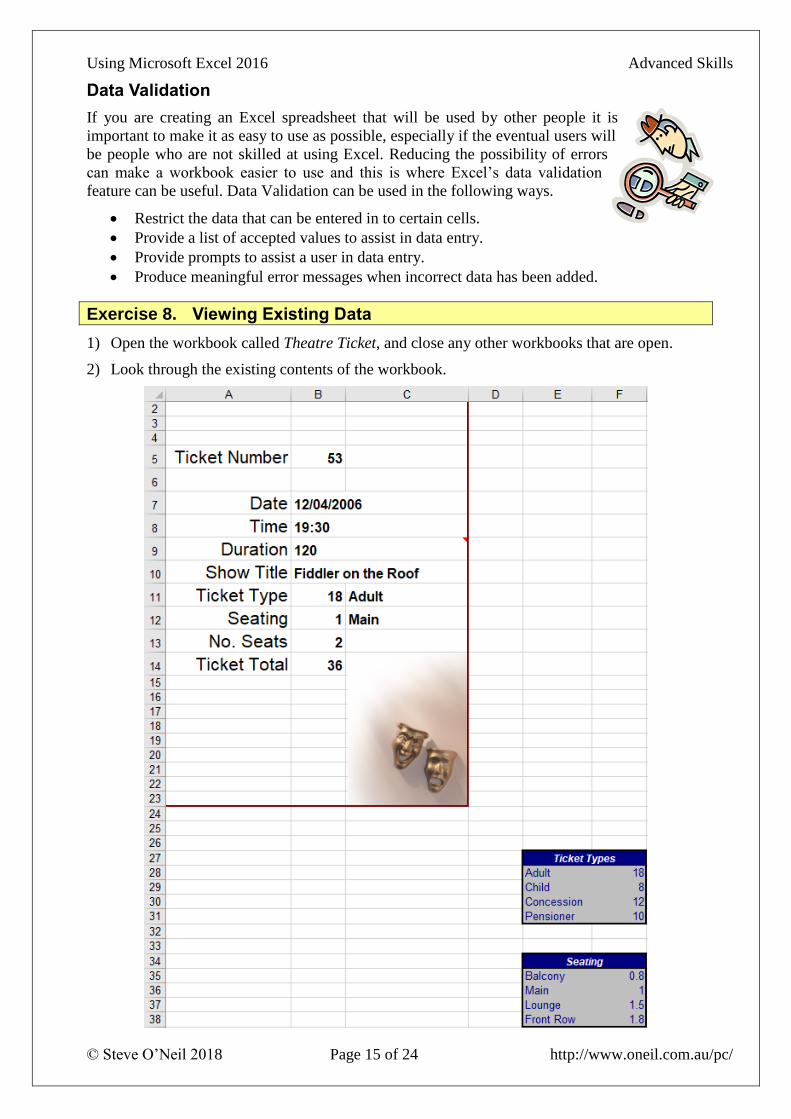
1) Open the workbook called Theatre Ticket, and close any other workbooks that are open.
2) Look through the existing contents of the workbook.
Using Microsoft Excel 2016 Advanced Skills
© Steve O’Neil 2018 Page 16 of 24 http://www.oneil.com.au/pc/
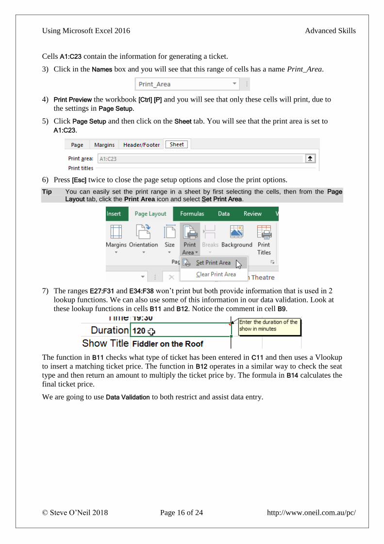
Cells A1:C23 contain the information for generating a ticket.
3) Click in the Names box and you will see that this range of cells has a name Print_Area.
4) Print Preview the workbook [Ctrl] [P] and you will see that only these cells will print, due to
the settings in Page Setup.
5) Click Page Setup and then click on the Sheet tab. You will see that the print area is set to
A1:C23.
6) Press [Esc] twice to close the page setup options and close the print options.
Tip You can easily set the print range in a sheet by first selecting the cells, then from the Page Layout tab, click the Print Area icon and select Set Print Area.
7) The ranges E27:F31 and E34:F38 won’t print but both provide information that is used in 2
lookup functions. We can also use some of this information in our data validation. Look at
these lookup functions in cells B11 and B12. Notice the comment in cell B9.
The function in B11 checks what type of ticket has been entered in C11 and then uses a Vlookup
to insert a matching ticket price. The function in B12 operates in a similar way to check the seat
type and then return an amount to multiply the ticket price by. The formula in B14 calculates the
final ticket price.
We are going to use Data Validation to both restrict and assist data entry.

Using Microsoft Excel 2016 Advanced Skills
© Steve O’Neil 2018 Page 17 of 24 http://www.oneil.com.au/pc/
Exercise 9. Adding Data Validation Rules
1) Select cell B9. This cell contains the duration of the show in minutes. Since none of the
shows go for longer than 200 minutes, we can put in a validation rule which restricts the data
that can be entered.
2) Select the Data tab on the Ribbon.
3) Click the Data Validation icon (if you click the top part of the icon you won’t need to
select from the menu of options and will go straight to data validation). A dialog box
like the one below will appear.
4) Change Allow to Whole Number. This will restrict the cell so that only whole numbers with
no decimals can be entered.
5) Change Data to less than or equal to.
6) When the Maximum box appears, enter 200 in the box to set that as the upper limit. In
addition to entering a number in this box you can also select a cell in your workbook which
has a suitable value. The options should now look like the example above.
The Input Message tab allows us to enter a popup prompt that will appear when the cell is
selected. Since the cell already has a comment, we’ll leave the Input message for this cell blank.
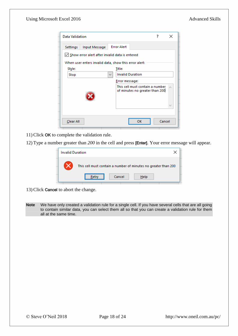
7) Click the Error Alert tab.
In this tab we can create a custom error message that will appear if the user enters a value not
allowed under the Validation Criteria. In this case, the error message will appear if a number
greater than 200 is entered, so we can create an error message appropriate for that situation.
The Style options determine the type of error message that will appear.
For instance, a Stop style error message will prevent the entry of
invalid data while the other types are only warnings.
8) Make sure the Style is set to Stop.
9) In the Title enter Invalid Duration.
10) For the Error Message type, “This cell must contain a number of minutes no greater than
200”. The options should look like the example below.
Using Microsoft Excel 2016 Advanced Skills
© Steve O’Neil 2018 Page 18 of 24 http://www.oneil.com.au/pc/
11) Click OK to complete the validation rule.
12) Type a number greater than 200 in the cell and press [Enter]. Your error message will appear.
13) Click Cancel to abort the change.
Note We have only created a validation rule for a single cell. If you have several cells that are all going to contain similar data, you can select them all so that you can create a validation rule for them all at the same time.

Using Microsoft Excel 2016 Advanced Skills
© Steve O’Neil 2018 Page 19 of 24 http://www.oneil.com.au/pc/
Exercise 10. Create Data Validation Lists
1) Select cell C11. This cell should contain the ticket type.
2) Click the Data Validation icon and make sure the Settings tab is showing.
3) Change the Allow option to List.
The Source box will appear. This allows us to provide a list of numbers or labels that will be
accepted. Anything entered that doesn’t match something in our list will produce an error. We
can either type in each of the entries separated by a comma or select a range of cells which has
an appropriate value in each cell. Since we already have a suitable range of cells being used in
the Vlookup function, we can also use it for a data validation list.
4) Click in the source box and make sure you can see the Ticket Types table in cells E28:F31
(you can still scroll down when the Data Validation options are showing). If you can’t see it,
you can click the icon to the right of the source box to temporarily hide the dialog box.
5) Select cells E28:E31. The cell references will appear in the source box. If you hid the Data
Validation Dialog in the previous step, click the icon to display it again.
6) Make sure the In-cell dropdown option is selected. This will mean that when the cell is
selected, a dropdown list of the allowable data will appear to make data entry easier. The
options should look like the example above.

Using Microsoft Excel 2016 Advanced Skills
© Steve O’Neil 2018 Page 20 of 24 http://www.oneil.com.au/pc/
7) Change the Input Message options so that they look like the example below.
8) Change the Error Alert options to look like the example below.
9) Click OK to complete the validation rule.
While the cell is selected, your input message will be visible next to the cell.
A dropdown arrow list will also appear next to the cell. If a value is entered in the cell which
doesn’t match an item in the ticket types list, a warning message will appear.
10) Select a ticket type from the dropdown list. Notice that all of the formulae in the worksheet
recalculate based on the changed information.
Using Microsoft Excel 2016 Advanced Skills
© Steve O’Neil 2018 Page 21 of 24 http://www.oneil.com.au/pc/
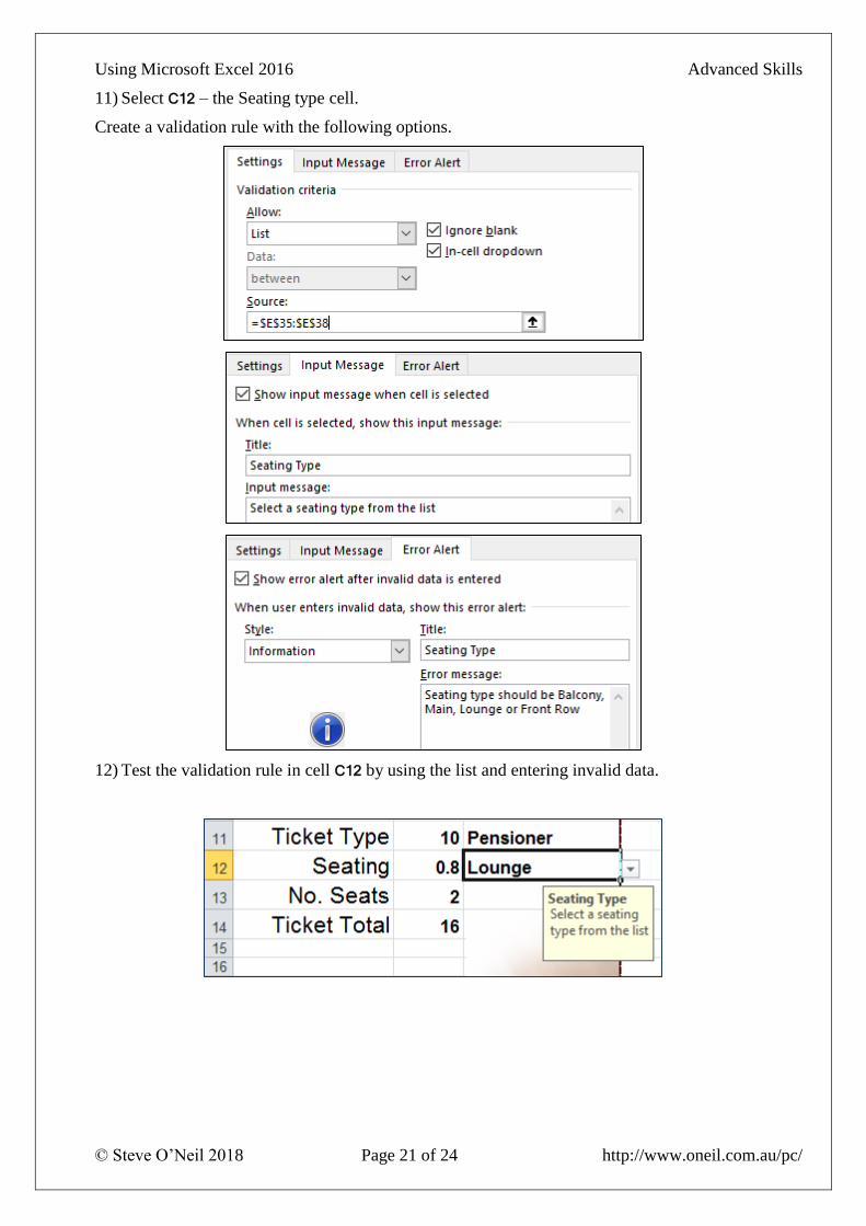
11) Select C12 – the Seating type cell.
Create a validation rule with the following options.
12) Test the validation rule in cell C12 by using the list and entering invalid data.

Using Microsoft Excel 2016 Advanced Skills
© Steve O’Neil 2018 Page 22 of 24 http://www.oneil.com.au/pc/
Custom Number Formats
In the Exercise on formatting we created some custom number formats. In the following
exercises we’re going to create some additional custom number formats using the ticket
workbook.
Exercise 11. Creating Custom Date and Time Formats
1) Select the date in cell B7.
2) Select Press [Ctrl] [1] shortcut.
3) Make sure the Number tab is selected.
4) Select Custom from the Category list.
5) Under Type, delete whatever is currently in there. The list below that contains several
existing custom formats and will also keep any that you create so they can be reused later.
6) Enter the following custom date code.
7) Click OK to apply the custom format. The date in the cell will now take on the new format.
8) Select B8, the time cell.
9) Create the following custom time format for that cell.
The format should make the time in the cell look like the following example.
7:30 PM
Using Microsoft Excel 2016 Advanced Skills
© Steve O’Neil 2018 Page 23 of 24 http://www.oneil.com.au/pc/
Exercise 12. Creating Custom Number Formats
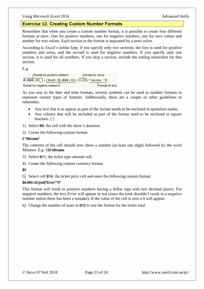
Remember that when you create a custom number format, it is possible to create four different
formats at once. One for positive numbers, one for negative numbers, one for zero values and
another for text values. Each section in the format is separated by a semi colon.
According to Excel’s online help, if you specify only two sections, the first is used for positive
numbers and zeros, and the second is used for negative numbers. If you specify only one
section, it is used for all numbers. If you skip a section, include the ending semicolon for that
section.
E.g.
As you saw in the date and time formats, several symbols can be used in number formats to
represent certain types of formats. Additionally, there are a couple of other guidelines to
remember.
• Any text that is to appear as part of the format needs to be enclosed in quotation marks.
• Any colours that will be included as part of the format need to be enclosed in square
brackets. [ ]
1) Select B9, the cell with the show’s duration.
2) Create the following custom format.
0 "Minutes"
The contents of the cell should now show a number (at least one digit) followed by the word
Minutes. E.g. 120 Minutes
3) Select B11, the ticket type amount cell.
4) Create the following custom currency format.
$0
5) Select cell B14, the ticket price cell and enter the following custom format.
$#,##0.00;[red]"Error";"0"
This format will result in positive numbers having a dollar sign with two decimal places. For
negative numbers, the text Error will appear in red (since the total shouldn’t result in a negative
number unless there has been a mistake). If the value of the cell is zero a 0 will appear.
6) Change the number of seats in B13 to test the format for the ticket total.

Using Microsoft Excel 2016 Advanced Skills
© Steve O’Neil 2018 Page 24 of 24 http://www.oneil.com.au/pc/
7) Save your workbook and try these custom formats on a blank worksheet and enter data in to
the cells to test the formats.
Format Suggested test data
"Remaining balance is" $#,##0.00 Any number
h:mm AM/PM "-" dd mmmm yyyy -now() function to calculate current date/time
$0.00;[red]$0.00;"Zero";[green]@ + and – numbers, 0, text
$* #,##0.00 " Debit";[Red]$* (#,##0.00)" Credit" + and – numbers
"You owe" 0 "dollars"; "You owe" -0 "dollars" Any number
Tip Custom number formats can also be used in some other applications. For instance, they are very useful for formatting data in Microsoft Access databases.