USING HOMOTOPY METHODS TO SOLVE

NONSMOOTH EQUATIONS

by

Adam Speight

B.S., University of Colorado at Denver, 1997

A thesis submitted to the

University of Colorado at Denver

in partial fulfillment

of the requirements for the degree of

Master of Science

Applied Mathematics

1999

This thesis for the Master of Science

degree by

Adam Speight

has been approved

by

Stephen C. Billups

Harvey J. Greenberg

Gary A. Kochenberger

Date

Speight, Adam (M.S., Applied Mathematics)

Using Homotopy Methods to Solve Nonsmooth Equations

Thesis directed by Professor Stephen C. Billups

ABSTRACT

This thesis presents a new method for solving nonsmooth systems of

equations, which is based on probability one homotopy techniques for solving

smooth equations. The method is based on a new class of homotopy mappings

on locally Lipschitz continuous operators that employ smoothing techniques to

ensure the homotopy map is smooth on its natural domain. The new homotopy

method is embedded in a hybrid algorithm. This is done so it may exploit the

strong global convergence properties of homotopy methods, while relying on

a Newton method for local converge to avoid potential numerical problems

associated with nonsmoothness nearby a solution. Several theoretical results

regarding the convergence behavior of this class of homotopy methods are

presented.

The hybrid algorithm is applied to solve problems from a class of

nonsmooth equations arising from a particular reformulation of the Mixed

Complementarity Problem. This paper presents computational results from

experimentation with the algorithm as well as issues related to the algorithm’s

implementation.

iii

In addition to presenting the hybrid algorithm, this thesis develops a

suite of software routines in the MATLAB environment that allows developers

to quickly create and evaluate homotopy-based solvers for nonsmooth equa-

tions. This software provides routines to help reformulate Mixed Complemen-

tarity Problems into nonsmooth equations, and an interface by which users may

solve complementarity problems specified in the GAMS modeling language. It

also includes interfaces to several sophisticated routines from HOMPACK90, a

well-established collection of FORTRAN90 codes for implementing homotopy

methods.

This abstract accurately represents the content of the candidate’s thesis. I

recommend its publication.

SignedStephen C. Billups

iv

ACKNOWLEDGMENTS

My most sincere thanks go to my advisor, Stephen Billups. For sev-

eral years, he has been a constant source of advice, guidance, friendship, and

inspiration, without which this thesis would never have been produced.

I would also like to offer my heartfelt thanks to Gary Kochenberger

for serving on my thesis committee and Harvey Greenberg for the same and

for providing many valuable comments, which greatly improved the quality of

this thesis. Thanks also goes to Layne Watson for his valuable suggestions.

During the course of my education, several teachers have infused me

with a drive to become more than I am and helped me acquire the means to

do so. To these individuals, I am eternally grateful. In particular, would like

to thank James Smith for helping me to discover a larger world, Allen Holder

for acquainting me with it, and David Fischer, Burton Simon, and Stephen

Medema for giving me the grand tour.

Thanks go to the faculty, staff, and students of the mathematics de-

partment at the University of Colorado at Denver who have provided me a

supportive and pleasant environment from which to develop. Thanks also go

to the Viotti family for helping me to keep perspective on what is really im-

portant in life.

Finally, I wish to thank my Family for years of support and prayers.

Without them I surely would not enjoy the richness of life that I do today.

CONTENTS

Figures . . . . . . . . . . . . . . . . . . . . . . . . . . . . . . . . . . . i

Tables . . . . . . . . . . . . . . . . . . . . . . . . . . . . . . . . . . . . i

1. Introduction . . . . . . . . . . . . . . . . . . . . . . . . . . . . . . . 1

2. Background Material . . . . . . . . . . . . . . . . . . . . . . . . . . 4

2.1 Notation . . . . . . . . . . . . . . . . . . . . . . . . . . . . . . . . 4

2.2 Applications of Nonsmooth Equations . . . . . . . . . . . . . . . 5

2.2.1 Inequality Feasibility Problem . . . . . . . . . . . . . . . . . . . 6

2.2.2 Nonlinear Complementarity Problem . . . . . . . . . . . . . . . 6

2.2.3 Variational Inequalities . . . . . . . . . . . . . . . . . . . . . . . 7

2.3 The Mixed Complementarity Problem . . . . . . . . . . . . . . . 8

2.3.1 Walrasian Equilibrium . . . . . . . . . . . . . . . . . . . . . . . 8

2.4 MCP Reformulation . . . . . . . . . . . . . . . . . . . . . . . . . 10

2.5 Newton’s Method . . . . . . . . . . . . . . . . . . . . . . . . . . . 12

2.5.1 Nonsmooth Newton Methods . . . . . . . . . . . . . . . . . . . 15

2.6 Homotopy Methods . . . . . . . . . . . . . . . . . . . . . . . . . . 17

2.6.1 Theory and Definitions . . . . . . . . . . . . . . . . . . . . . . . 18

2.6.2 Homotopy-based Algorithms . . . . . . . . . . . . . . . . . . . . 22

2.7 Dealing with nonsmoothness . . . . . . . . . . . . . . . . . . . . . 28

2.7.1 Complementarity Smoothers . . . . . . . . . . . . . . . . . . . . 29

3. The Algorithm . . . . . . . . . . . . . . . . . . . . . . . . . . . . . 33

vi

3.1 The Algorithm . . . . . . . . . . . . . . . . . . . . . . . . . . . . 34

3.2 Properties of %a . . . . . . . . . . . . . . . . . . . . . . . . . . . . 35

3.3 A Hybrid Algorithm . . . . . . . . . . . . . . . . . . . . . . . . . 38

3.4 Solving Mixed Complementarity Problems . . . . . . . . . . . . . 40

4. Implementation . . . . . . . . . . . . . . . . . . . . . . . . . . . . . 42

4.1 HOMTOOLS . . . . . . . . . . . . . . . . . . . . . . . . . . . . . 42

4.1.1 The Root Finding Package. . . . . . . . . . . . . . . . . . . . . 44

4.1.2 The Utility Package. . . . . . . . . . . . . . . . . . . . . . . . . 49

4.1.3 The Homotopy Smooth Package. . . . . . . . . . . . . . . . . . 50

4.1.4 The MCP Smooth Package. . . . . . . . . . . . . . . . . . . . . 51

4.1.5 The GAMS MCP Package. . . . . . . . . . . . . . . . . . . . . 53

4.1.6 The Algorithms Package. . . . . . . . . . . . . . . . . . . . . . . 54

4.2 Solver Implementation . . . . . . . . . . . . . . . . . . . . . . . . 55

5. Results and Conclusions . . . . . . . . . . . . . . . . . . . . . . . . 57

5.1 Testing Procedure . . . . . . . . . . . . . . . . . . . . . . . . . . 57

5.2 Computational Results . . . . . . . . . . . . . . . . . . . . . . . . 61

5.3 Conclusions . . . . . . . . . . . . . . . . . . . . . . . . . . . . . . 61

5.4 Avenues for Further Research . . . . . . . . . . . . . . . . . . . . 62

References . . . . . . . . . . . . . . . . . . . . . . . . . . . . . . . . . . 64

vii

FIGURES

Figure

2.1 A nonsmooth Newton’s method with line search . . . . . . . . . 14

2.2 A smoother for max(x, 0) . . . . . . . . . . . . . . . . . . . . . . 30

3.1 A hybrid algorithm . . . . . . . . . . . . . . . . . . . . . . . . . 39

3.2 Procedure to evaluate an element of ∂BH(x) . . . . . . . . . . . 41

viii

TABLES

Table

4.1 Parameters for a HOMTOOLS compliant solver . . . . . . . . . 45

4.2 Overview of the HOMTOOLS public interface . . . . . . . . . . 46

5.1 MCPLIB Test Problems . . . . . . . . . . . . . . . . . . . . . . 58

5.2 MCPLIB Test Problems (continued) . . . . . . . . . . . . . . . 59

5.3 MCPLIB Test Problems (continued) . . . . . . . . . . . . . . . 60

ix

1. Introduction

The problem of solving systems of equations is central to the field of

applied mathematics. Many robust and efficient techniques exist to solve sys-

tems that are linear or differentiable. In recent years, however, there has been

an increasing need for techniques to solve systems of equations that are nons-

mooth, i.e., not continuously differentiable. Much progress has been made in

generalizing Newton’s method to solve such systems [16]. Techniques developed

in this vein are attractive because they maintain the fast local convergence

properties that are characteristic of Newton-based methods for smooth equa-

tions and perform with great efficacy when applied to nonsmooth problems

that are nearly linear in the sense that their merit functions do not contain

local minima that are not solutions. For problems that are highly nonlinear,

however, these Newton-based schemes tend to fail or require a carefully chosen

starting point to produce a solution. Finding such a point may require a great

deal of human intervention.

To solve highly nonlinear systems of equations that are smooth, an-

other class of algorithms known as homotopy methods may be employed, which

often prove more robust than their Newton-based counterparts. To date very

little progress has been made in extending homotopy methods into the domain

of solving nonsmooth systems of equations. A principle objective of this thesis

is to develop a class of techniques that extend conventional homotopy methods

so they can be made to solve nonsmooth systems. A secondary objective of this

thesis is to develop a set of software tools that allows for the rapid prototyping,

1

development, and testing of homotopy-based solvers for nonsmooth equations.

Chapter 2 presents some applications of nonsmooth systems of equa-

tions and describes a Newton-based method to solve them. It then presents

some background material that will be necessary for the remainder of the the-

sis, including some theory on probability one homotopy methods for smooth

equations, algorithms for implementing the same, and some theory about

smoothing techniques for nonsmooth functions.

Chapter 3 describes our approach for using homotopy methods for

solving nonsmooth equations. It presents some theoretical results, stating suf-

ficient conditions under which the method should find a solution and discusses

how the method can be incorporated into a hybrid algorithm, which makes use

of a Newton-based method to achieve fast local convergence.

Chapter 4 details a suite of MATLAB software called HOMTOOLS.

This package provides a uniform framework by which algorithm developers

may write homotopy-based solvers for nonsmooth systems in MATLAB and

other environments and test them against sets of problems coming from a va-

riety of sources, including GAMS. It also makes several of the routines from

the HOMPACK90 suite of codes available in the MATLAB environment. This

package provides several sophisticated routines pertinent to homotopy-based

algorithms that allow developers to leverage highly sophisticated routines and

quickly write high-level algorithms. Chapter 4 also discusses how the homo-

topy method presented in Chapter 3 was implemented and integrated with

HOMTOOLS.

Chapter 5 presents some computational results obtained from exper-

imenting with the algorithm described in Chapters 3 and 4. It attempts to

discern why the algorithm failed when it did and characterize the algorithm’s

2

potential for usefulness in the future. This chapter concludes with a discussion

on some future avenues for research.

3

2. Background Material

2.1 Notation

When discussing matrices, vectors and vector-valued functions, sub-

scripts are used to indicate components, whereas superscripts are used to indi-

cate the iteration number or some other label. For example Ai·, A·j, Aij refer to

the ith row, jth column, and (i, j)th entry of a matrix A, respectively, whereas

xk typically represents the kth iterate generated by an algorithm. In contrast

to the above, for scalars or scalar-valued functions, we use subscripts to refer

to labels so that superscripts can be reserved for exponentiation. The vector

of all ones is represented by e.

Unless otherwise specified, ‖·‖ denotes the Euclidean norm. We use

the notation (·)+, (·)−, and | · | to represent the plus, minus, and absolute value

operators, respectively, for vectors. That is, x+ := (max(x1, 0); . . . ; max(xn, 0)),

x− := (max(−x1, 0); . . . ; max(−xn, 0)), and |x| := (|x1|; . . . ; |xn|).

The symbols <+ and <++ refer to the nonnegative real numbers and

the positive real numbers respectively. The extended real numbers are denoted

by < := <⋃{−∞,+∞}. The vectors l and u ∈ < n, specify a set of lower and

upper bounds. Throughout this thesis we assume that l < u. The symbol Bl,urepresents the box defined by [l, u] := {x | l ≤ x ≤ u}.

Real-valued functions are denoted with lower-case letters like f or φ

whereas vector-valued functions are represented by upper-case letters like F

or Φ. For a function F : C ⊂ <n → <m, we define ∇iFj(x) := ∂Fj(x)/∂xi.

∇F (x) is the n × m matrix whose ijth element is ∇iFj(x). Thus, if f is a

4

scalar valued function, then ∇f(x) is a row vector.

For a set C ⊂ <n we denote its closure and boundary by C and ∂C

respectively. The projection operator for the set C is denoted by πC(·). That

is, πC(x) represents the projection (with respect to the Euclidean norm) of x

onto the set C.

We will use the notation o(·) as follows: given a function H : <n →

<m, o(H(x)) to represents any function G : <n → <s satisfying

lim‖x‖→0

‖G(x)‖‖H(x)‖

= 0.

A sequence is said to converge quadratically if

lim supk→∞

∥∥∥xk+1 − x∗∥∥∥

‖xk − x∗‖2 <∞

and superlinearly if

lim supk→∞

∥∥∥xk+1 − x∗∥∥∥

‖xk − x∗‖= 0.

We say that two sets, A and B, are diffeomorphic if there is a con-

tinuously differentiable bijection β : A→ B such that β−1 is also continuously

differentiable. The term ’almost everywhere’ will be used to modify to proper-

ties indicating that they hold on all elements of a set except on a subset having

zero Lesbegue measure.

2.2 Applications of Nonsmooth Equations

The need to solve nonlinear equations arises frequently in the field of

mathematical and equilibrium programming as well elsewhere in applied math-

ematics and in several engineering disciplines. In [16] a number of applications

for nonsmooth equations are presented; some of which are described in this

section.

5

2.2.1 Inequality Feasibility Problem Finding solutions to sys-

tems of inequalities is an important and often difficult task in applied math-

ematics. Suppose F : <n → <n is a locally Lipschitzian function and K is a

polyhedral region in <n. The inequality feasibility problem is to find an x ∈ K

such that

F (x) ≥ 0. (2.1)

We can reformulate this into a system of equations by letting

H(x) = min(0, F (x)),

where min(·, . . . , ·) is the componentwise minimum function of a finite number

of vectors. It is clear that H is a nonsmooth operator and that x∗ solves (2.1)

if, and only if, H(x∗) = 0.

2.2.2 Nonlinear Complementarity Problem The nonlinear

complementarity problem (NCP) is a tool commonly used to model equilibrium

problems arising in economics and game theory. It also serves as a generalized

framework for many of the problems faced in mathematical programming. Giv-

en a continuously differentiable function F : <n → <n, the problem NCP(F )

is to find some x ∈ <n so that

0 ≤ x ⊥ F (x) ≥ 0 (2.2)

where x ⊥ F (x) means that xTF (x) = 0.

We may take several approaches to reformulate the problem NCP(F )

into a nonsmooth system of equations. Define the functions

Hm(x) = min(x, F (x)), (2.3)

HN(x) = F (x+)− x−, and (2.4)

6

HFB(x) =(xi + Fi(x)−

√x2i + Fi(x)2

)(2.5)

where the x+i := max(xi, 0) and x−i := −min(xi, 0) . One may easily

verify that the following are equivalent:

(1) x∗ solves (2.2),

(2) Hm(x∗) = 0,

(3) HN(z) = 0 where x∗ = z+, and

(4) HFB(x∗) = 0.

2.2.3 Variational Inequalities Finite dimensional variational

inequalities provide a framework from which to generalize the nonlinear com-

plementarity problem as well as other problems in mathematical programming.

A comprehensive treatment of the variational inequality is available in [12].

Suppose K is some closed convex subset of <n and F : D → <n is a differen-

tiable function over some open domain D ⊂ <n containing K. The problem

VI(K,F ) is to find some x∗ ∈ <n so that

(y − x∗)TF (x∗) ≥ 0 for every y ∈ K. (2.6)

To reformulate VI(F,K) into a system of equations we may define

the following functions in terms of the Euclidean projection operator π, which

induces the nonsmoothness in the reformulations:

Hm(x) = x− πK(x− F (x)), and (2.7)

HN(x) = F (πK(x)) + (x− πK(x)). (2.8)

The notation for these functions is identical to those defined in (2.3)

and (2.4) because if K = <n+ the function Hm in (2.3) is equivalent to the

function Hm in (2.7) and the function HN in (2.4) is equivalent to HN in (2.8).

The function HN is sometimes referred to as the normal map. That solving

these equations is equivalent to solving VI(F,K) is shown in [12, Chapter 4].

7

2.3 The Mixed Complementarity Problem

One prominent class of problems we are interested in solving is the

Mixed Complementarity Problem (MCP). Some prefer to refer to the MCP as

the box-constrained variational inequality. This class of problems generalizes

the NCP (Section 2.2.2) in that any component of the solution may be bounded

above, bounded below, both, or unbounded altogether. We can reformulate the

MCP into a system of nonsmooth equations in a fashion similar to the NCP

reformulations. This thesis will pay particular attention to applying homotopy-

based algorithms to a particular reformulation of this problem.

Given a rectangular region Bl,u :=∏ni=1[li, ui] in (<∪{±∞})n defined

by two vectors, l and u in <n where −∞ ≤ l < u ≤ ∞, and a function

F : Bl,u → <n, the Mixed Complementarity Problem MCP(F,Bl,u) is to find

an x ∈ Bl,u such that for each i ∈ {1, . . . , n}, either

(1) xi = li, and Fi(x) ≥ 0, or

(2) Fi(x) = 0, or

(3) xi = ui, and Fi(x) ≤ 0.

This is equivalent to the condition that the componentwise median function,

mid(x − l, x − u, F (x)) = 0. Sometimes when these conditions are satisfied

we write F (x) ⊥ x and say that x is complementary to F (x). Typically, one

assumes that the function F above is continuously differentiable on some open

set containing Bl,u.

2.3.1 Walrasian Equilibrium MCPs are useful for modeling

systems that have many agents, each of whom is optimizing a function. These

functions may be interdependent in that the choice variables of all the agents

may be parameters in the objective function of each agent. These interde-

pendent systems of nonlinear programs may be reformulated into an MCP by

8

viewing the combined Karush-Kuhn-Tucker conditions of each agent’s problem

as one large system of inequalities and noticing that together these systems

form one large MCP. This reformulation is useful for recasting and solving

many models arising in game theory and economics.

Of particular interest to microeconomists is the topic of general eco-

nomic equilibrium. General equilibrium models usually incorporate many con-

sumers, each of whom are maximizing their own utility and a production mech-

anism usually consisting of firms who are profit maximizers. A Walrasian

equilibrium is characterized by having a set of prices, production activities,

and consumption activities such that no good is in positive excess demand [19,

Chapter 17.2].

Suppose there are m consumers in an economy and they may choose

to purchase from a set of n goods, which can be purchased in arbitrarily fine

quantities. If each consumer has well-behaved preferences then m quasi-convex

utility functions (ui : <n → <, i = 1 . . .m) exist describing the consumers’

preferences[19]. If each consumer has an initial endowment of goods Ei ∈

<n, i = 1 . . .m, and p ∈ <n is a given vector of prices, then the ith consumer

faces the following problem:

maximizex≥0 ui(x)

subject to p · x ≤ p · Ei.(2.9)

Solving each of these m nonlinear programs parametrically in terms of the

price vector p gives rise to demand operators for each consumer, di(p), where

dij(p) is the amount of good j that consumer i will consume at price level p

[19, Chapter 7].

For the production side of the model, suppose there are k production

sectors. Each sector j has an associated production level yj that produces some

9

amount (possibly negative) of each good. It is usual to assume that production

is linear; that is the set of producible goods is a convex cone in <n [15]. If

vectors of output y and z can be produced, then so can any combination αy+βz

where α and β are nonnegative scalars. Because there are a finite number of

production sectors, the production cone is also an unbounded polyhedron, so

we may represent the production set by a technology matrix A ∈ <n×k. The

element Aij represents the amount of good i resulting in a unit of activity in

sector j.

A set of equilibrium conditions adapted from [18] follows.

No activity earns a positive profit: pTA ≤ 0 (1)

No good is in excess demand:∑mi=1 d

i(p)−∑mi=1 E

i − Ay ≤ 0 (2)

Positive prices and production: p ≥ 0, y ≥ 0 (3)

No losses or positive profits:(pTA

)y = 0 (4)

Goods in excess supply are free

and all goods with positive price

are sold: pT (∑mi=1 E

i + Ay −∑mi=1 d

i(p)) = 0 (5)

The equations (4) and (5) indicate that the inequality (1) is complementary

to y and the inequality (2) is complementary to p. The above system can be

viewed as a Nonlinear Complementarity Problem because each component of

y and p is bounded by 0 and infinity.

2.4 MCP Reformulation

This section describes a class of operators such that any root of a

particular operator is a solution to an associated MCP and any solution to

that MCP is a root of its operator. Classes of both smooth and nonsmooth

operators exist with this property, each with its own advantages. This section

10

focuses on a class of nonsmooth reformulations of a generic MCP.

Definition 2.4.1 A function φ : <2 → < is called an NCP function if φ(a, b) =

0 if and only if min(a, b) = 0.

These functions are so named because they are useful in reformulating

NCPs (see Section 2.2.2). Equation (2.3) describes one way to reformulate an

NCP using the component-wise minimum function, each component of which

is trivially an NCP function. Indeed, this reformulation would still hold if the

H defined in (2.3) were instead defined by

Hi(x) = φ(xi, fi(x))

where φ is any NCP function.

Definition 2.4.2 A function ψ : <∪{−∞}×<∪{∞}×<2 → < is called an

MCP function associated with l and u if ψl,u(x, f) := ψ(l, u, x, f) = 0 if and

only if mid(x− l, x− u, f) = 0.

MCP functions are generalized NCP functions. If the lower bound l is zero

and upper bound u is infinite, then the MCP function ψl,u(x, f) is also an

NCP function because

0 = mid(x− l, x− u, f) = mid(x,−∞, f) = min(x, f)

if, and only if, ψl,u(x, f) = 0.

One very popular NCP function is the Fischer-Burmeister function

[9, 10],

φFB(a, b) := a+ b−√a2 + b2. (2.10)

A simple check reveals that this is an NCP function. While φFB is not dif-

ferentiable at the origin, φ2FB has the desirable property of being continuously

differentiable everywhere. This property makes the Fischer-Burmeister func-

tion well suited for use in globalization strategies for Newton-based methods.

11

The function φFB is also semismooth (see Definition 2.5.3). This fact will

be useful when we solve systems of semismooth equations incorporating the

Fischer-Burmeister function.

Using either the pairwise minimum function or the Fischer-Burmeister

function as φ, Billups [1] was able to construct the MCP function:

ψ(l, u, x, f) := φ(x− l,−φ(u− x,−f)). (2.11)

Constructing a function H : <n → <n from a box Bl,u defined by

vectors l and u and a C2 operator F,

Hi(x) := ψ(li, ui, xi, Fi(x)) (2.12)

yields a reformulation of the MCP(F,Bl,u). H(x) = 0 if and only if x is a

solution to MCP(Bl,u, F )[1]. Solving the nonsmooth equation H(x) = 0 will

be the focus of much attention in later chapters.

2.5 Newton’s Method

Newton’s method is a standard technique for solving the equation

F (x) = 0. (2.13)

If F : <n → <n is a continuously differentiable, or smooth, operator and x0 is

a starting point in <n, the sequence of iterates

xk+1 := xk − [∇F (xk)]−1F (xk), k = 0, 1, . . . (2.14)

is well-defined and converges quadratically under conditions summarized in the

following theorem.

Theorem 2.5.1 [7]. Let F : <n → <n be continuously differentiable in an

open convex set D ⊂ <n. Assume there is some x∗ ∈ <n and r, β > 0, so

12

that IBr(x∗) ⊂ D,F (x∗) = 0,∇F (x∗)−1 exists with ‖∇F (x∗)−1‖ ≤ β and ∇F

is Lipschitz continuous with constant γ on IBr(x∗). Then, there exists some

ε > 0 such that for every x0 ∈ IBr(x∗) the sequence generated by (2.14) is well

defined, converges to x∗, and obeys

∥∥∥xk+1 − x∗∥∥∥ ≤ γβ

∥∥∥xk − x∗∥∥∥2k = 0, 1, . . . .

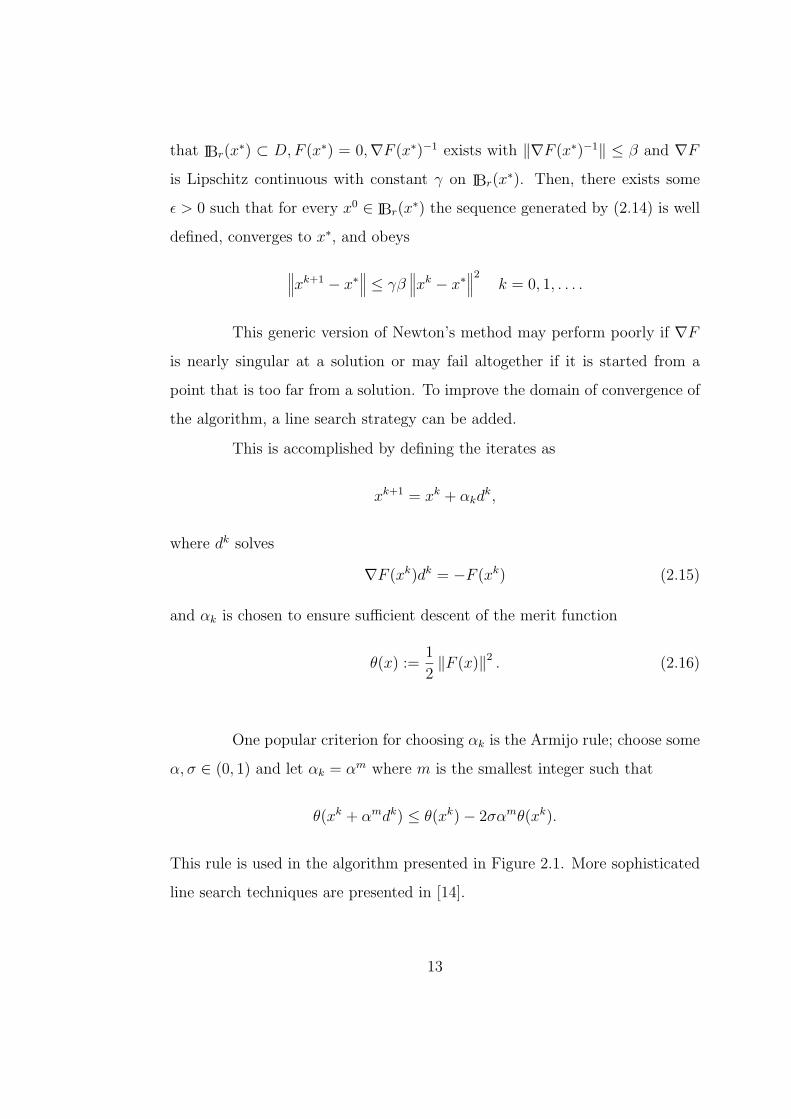
This generic version of Newton’s method may perform poorly if ∇F

is nearly singular at a solution or may fail altogether if it is started from a

point that is too far from a solution. To improve the domain of convergence of

the algorithm, a line search strategy can be added.

This is accomplished by defining the iterates as

xk+1 = xk + αkdk,

where dk solves

∇F (xk)dk = −F (xk) (2.15)

and αk is chosen to ensure sufficient descent of the merit function

θ(x) :=1

2‖F (x)‖2 . (2.16)

One popular criterion for choosing αk is the Armijo rule; choose some

α, σ ∈ (0, 1) and let αk = αm where m is the smallest integer such that

θ(xk + αmdk) ≤ θ(xk)− 2σαmθ(xk).

This rule is used in the algorithm presented in Figure 2.1. More sophisticated

line search techniques are presented in [14].

13

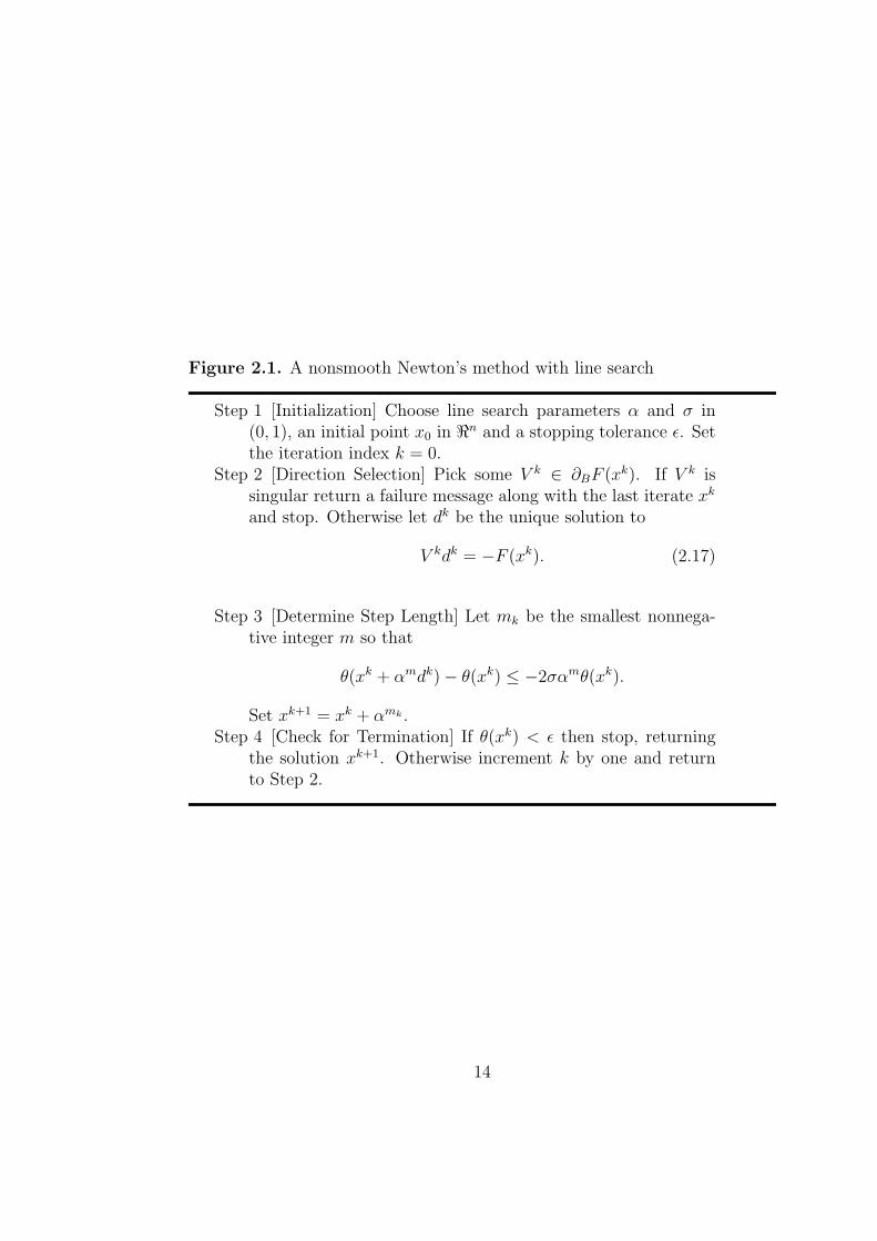
Figure 2.1. A nonsmooth Newton’s method with line search

Step 1 [Initialization] Choose line search parameters α and σ in(0, 1), an initial point x0 in <n and a stopping tolerance ε. Setthe iteration index k = 0.

Step 2 [Direction Selection] Pick some V k ∈ ∂BF (xk). If V k issingular return a failure message along with the last iterate xk

and stop. Otherwise let dk be the unique solution to

V kdk = −F (xk). (2.17)

Step 3 [Determine Step Length] Let mk be the smallest nonnega-tive integer m so that

θ(xk + αmdk)− θ(xk) ≤ −2σαmθ(xk).

Set xk+1 = xk + αmk .Step 4 [Check for Termination] If θ(xk) < ε then stop, returning

the solution xk+1. Otherwise increment k by one and returnto Step 2.

14

2.5.1 Nonsmooth Newton Methods Developing versions of

Newton’s method that require weaker assumptions regarding the differentia-

bility of F has been the focus of much research in recent years. Much of this

research attempts to assume only the property of semismoothness about F and

employs the notion of a generalized Jacobian or subdifferential whenever F is

not differentiable.

Definition 2.5.2 Let F : <n → <m be a locally Lipschitzian function. By

Rademacher’s Theorem, F is differentiable except on a set of Lesbegue measure

zero. Let DF be the set on which F is differentiable. Define the B-subdifferental

of F by

∂BF (x) :={V∣∣∣∣∃{xk} → x, xk ∈ DF , V = lim

k→∞∇F (xk)

}.

The Clarke subdifferential of F is the convex hull of ∂BF (x) and is denoted as

∂F (x).

It is clear that if F is differentiable at a point x, then either char-

acterization of the subdifferential is simply the singleton set containing only

∇F (x). In this regard, the subdifferential generalizes the gradient.

Definition 2.5.3 A function F : <n → <m is called semismooth at x if

lim

V ∈ ∂F (x+ th′)

h′ → h, t ↓ 0

{V h′}

exists for every h in <n.

The apparent awkwardness of the definition of semismoothness is due to the

fact that much of nonsmooth analysis requires a condition weaker than dif-

ferentiability to be useful and stronger than local Lipschitz continuity to be

powerful. Semismoothness is such a property. In [17], Qi presents some alter-

nate characterizations of semismoothness. The most intuitive interpretation,

15

however, is that semismoothness is equivalent to the uniform convergence of

directional derivatives in all directions. It is also worth noting that the class

of semismooth functions is closed under composition.

In [17], a version of Newton’s method based on the Clarke subdiffer-

ential was presented. To find a solution to the equation F (x) = 0, starting

from a point x0, the iterative map

xk+1 := xk −[V k]−1

F (xk), (2.18)

where V k ∈ ∂F (xk), may be followed.

An algorithm presented in [1, Figure 1] is outlined in Figure 2.1. It

presents an algorithm similar to the above Newton’s method but adds a line

search strategy and uses a merit function θ (for example θ(x) := 12‖F (x)‖2). It

also differs in that V k is restricted to be in the B-subdifferential, whereas [17]

uses the Clarke subdifferential. The convergence analysis for this particular

method uses the concepts of semicontinuity and BD-regularity.

Definition 2.5.4 Suppose that F : <n → <m is B-differentiable in a neigh-

borhood of x. We say that the directional derivative F ′(·; ·) is semicontinuous

at x if, for every ε > 0, there exists a neighborhood N of x such that, for all

x+ h ∈ N ,

‖F ′(x+ h;h)− F ′(x;h)‖ ≤ ε ‖h‖ .

We say that F ′(·; ·) is semicontinuous of degree 2 at x if there exist a constant

L and a neighborhood N of x such that, for all x+ h ∈ N ,

‖F ′(x+ h;h)− F ′(x;h)‖ ≤ L ‖h‖2 .

The following definition generalizes the notion of nonsingularity. In

nonsmooth analysis, regularity assumptions on functions are highly analogous

to the nonsingularity of Jacobians in the analysis of smooth operators.

16

Definition 2.5.5 A semismooth operator F is called BD-regular at x if every

element of ∂BF (x) is nonsingular.

The local convergence results for the nonsmooth Newton’s method

presented in Figure 2.1 are presented in the following theorem.

Theorem 2.5.6 [1] Suppose that x∗ is a solution to F (x) = 0, and that F

is semismooth and BD-regular at x∗. Then, the iteration method defined by

xk+1 = xk + dk, where dk is given by (2.17) is well defined and converges to x∗

superlinearly in a neighborhood of x∗. In addition, if F (xk) 6= 0 for all k, then

limk→∞

∥∥∥F (xk+1)∥∥∥

‖F (xk)‖= 0.

If, in addition, F is directionally differentiable in a neighborhood of x∗ and

F ′(·; ·) is semicontinuous of degree 2 at x∗, then the convergence of the itera-

tions is quadratic.

Newton-based methods perform well on problems whose merit functions do not

have non-zero local minima. For problems with higher degrees of nonlinearity,

Newton-based methods tend to stall by converging to a local minimum of their

merit function, or otherwise fail by diverging altogether. The local convergence

theory presented above guarantees that they will produce a solution within an

arbitrary tolerance provided that they are started sufficiently near to a solution.

For many highly nonlinear problems this is not practical, and a more robust,

globally convergent method is desired.

2.6 Homotopy Methods

A homotopy is a topological construction representing a function that

continuously deforms an element of a function space into another element of

that space. Suppose we are trying to solve the smooth equation F (x) = 0

17

where F : <n → <n. An example of a simple homotopy on F is

ρ(a, λ, x) := λF (x) + (1− λ)Ga(x)

where λ ∈ [0, 1] is called the homotopy parameter and a is some fixed vector

in <n. Here, Ga is some trivial class of operators on <n. An example may be

Ga(x) = x− a. It is clear that when λ = 1 we have that ρ(a, 1, x) = F (x) and

when λ = 0, ρ(a, 0, x) = Ga(x).

Much progress has been made in using the theory of homotopy map-

pings to construct techniques for finding zeros of smooth functions. This sec-

tion describes some theory of probability one homotopy methods and describes

a standard algorithm to implement them. The term ‘probability one’ applies

because under appropriate conditions, a path from the starting point, which

is uniquely determined by the parameter a, to a solution will fail to exist only

on a set of those a having zero Lesbegue measure.

2.6.1 Theory and Definitions Much of the theory from prob-

ability one homotopy methods can be derived from generalizations of a result

in fixed-point theory called Sard’s Theorem. This class of theorems uses a

notion of a regular value.

Definition 2.6.1 Let U ⊂ <n be open and F : <n → <m be a smooth

function. We say that y ∈ <m is a regular value of F if

Range ∇F (x) = <m, for all x ∈ F−1(y).

Theorem 2.6.2 (Parameterized Sard’s Theorem) [5] Let V ⊂ <q,

U ⊂ <m be open sets and let Υ : V × U → <p be of class Cr, where

r > max{0,m − p}. If 0 ∈ <p is a regular value of Υ, then for almost ev-

ery a ∈ V, 0 is a regular value of the function Υa defined by Υa(·) := Υ(a, ·).

18

Corollary 2.6.3 [5] Assume the conditions of the previous theorem. If m =

p + 1, then each component of Υ−1a ({0}) is a smooth curve for almost every

a ∈ V with respect to q-dimensional Lebesque measure.

The following proposition gives conditions under which a well-behaved zero

curve will exist. It is similar to results presented in [20] and [5, Theorem 2.4].

The path γa defined in the proposition ‘reaches a zero of F ’ in the sense that

it contains a sequence {(λk, xk)} that converges to (1, x), where x is a zero of

F .

Proposition 2.6.4 Let F : <n → <n be a Lipschitz continuous function and

suppose there is a C2 map

ρ : <m × [0, 1)×<n → <n

such that

(1) ∇ρ(a, λ, x) has rank n on the set ρ−1({0}),

(2) the equation ρa(0, x) = 0, where ρa(λ, x) := ρ(a, λ, x), has a unique solu-

tion xa ∈ <n for every fixed a ∈ <m,

(3) ∇xρa(0, xa) has rank n for every a ∈ <m,

(4) ρ is continuously extendable (in the sense of Buck [3]) to the domain

<m × [0, 1]×<n, and ρa(1, x) = F (x) for all x ∈ <n and a ∈ <m, and

(5) γa, the connected component of ρ−1a ({0}) containing (0, xa), is bounded

for almost every a ∈ <m.

Then for almost every a ∈ <m there is a zero curve γa of ρa, along which

∇ρa has rank n, emanating from (0, xa) and reaching a zero x of F at λ = 1.

Further, γa does not intersect itself and is disjoint from any other zeros of ρa.

Also, if γa reaches a point (1, x) and F is regular at x, then γa has finite arc

length.

19

Proof: Assumption 1 and the Parameterized Sard’s Theorem give that 0 is a

regular value of ρa for almost every a ∈ <m. By Corollary 2.6.3 each component

of(ρa|(0,1)×<n

)−1({0}) is a smooth curve and, as such, either diffeomorphic to a

circle or an interval [5]. Because ∇xρa(0, xa) has rank n, the Implicit Function

Theorem gives x in terms of λ in a neighborhood of (0, xa). This implies that

γa is not diffeomorphic to a circle. Since ρa is of class C2, all limit points of

γa must lie in ρ−1a ({0}) (with ρa’s extended domain <n × [0, 1] × <m), so the

only limit point of γa in {0} × <n is (0, xa). Furthermore, γa ∩ ((0, 1)×<n) is

diffeomorphic to an interval and (0, xa) corresponds to one end of it. Since γa

is bounded, there is some bounded closed set B ⊂ <n such that γa ⊂ [0, 1]×B.

By the Implicit Function Theorem, γa cannot terminate (have an end point)

in (0, 1) × <n, and by compactness γa has finite arc length in every compact

subset of [0, 1) × B. (For each point z ∈ γa, there is a neighborhood of z in

which γa has finite arc length by the Implicit Function Theorem and the fact

that 0 is a regular value of ρa. For z 6∈ γa, there is a neighborhood of z disjoint

from γa since <n is normal. These neighborhoods form an open covering of

[0, 1) × B, for which the finite subcovering of a compact subset [0, 1 − ε] × B

yields finite arc length for the portion of γa in [0, 1 − ε] × B.) Therefore γa

must leave every set [0, 1 − ε] × B, ε > 0, and have a limit point in {1} × B.

By continuity of ρa if (1, x∗) is a limit point of γa, then x∗ is a zero of F .

That γa does not intersect itself or any other component of ρ−1a ({0})

follows from the Implicit Function Theorem and the full rank of ∇ρa(λ, x) on

ρ−1a ({0}): for each z ∈ γa there is a neighborhood B(z) such that B(z) ∩ γa is

diffeomorphic to an open interval.

If (1, x) is a limit point of γa and F is regular at x, then every el-

ement of πx∂ρa(λ, x) is nonsingular. By the Implicit Function Theorem for

20

nonsmooth functions (see [6][Corollary, Page 256]), γa can be described as a

Lipschitz continuous function of λ in a neighborhood of (1, x), and therefore

has finite arc length in this neighborhood. Further, the zero curve has finite

arc length outside this neighborhood by the above argument, and hence finite

arc length everywhere.

A function such as ρ is called a homotopy mapping for F . The zero

curve γa described above can be characterized as the connected component of

the set ρ−1a ({0}) containing the point (0, xa). Because the path γa is a smooth

curve, it can be parameterized by its arc length away from (0, xa). This yields

a function γa(s), the point on γa of arc length s away from (0, xa).

Given a homotopy mapping ρ, we may construct a globally convergent

algorithm as follows. Choose an arbitrary a ∈ <m. This determines a unique

starting point x0. With probability one, we may then track the zero curve γa

to a point (1, x), where x is a solution.

A simple and particularly useful homotopy mapping is ρ : <n×[0, 1)×

<n → <n given by

ρ(a, λ, x) := λF (x) + (1− λ)(x− a). (2.19)

If F is a C2 operator then ρ satisfies properties (1), (2), (3), and (4) but not

necessarily (5) of Proposition 2.6.4. Properties (2), (3), and (4) are satisfied

trivially. That ρ satisfies property (1) can be seen in [21]. The following

theorem gives conditions on F under which the fifth condition is satisfied.

Theorem 2.6.5 [21] Let F : <n → <n be a C2 function such that for some

x ∈ <n and r > 0,

(x− x)TF (x) ≥ 0 whenever ‖x− x‖ = r. (2.20)

21

Then F has a zero in a closed ball of radius r about x, and for almost every a

in the interior of this ball there is a zero curve γa of

ρa(λ, x) := λF (x) + (1− λ)(x− a),

along which ∇ρa(λ, x) has full rank, emanating from (0, a) and reaching a zero

x of F at λ = 1. Further, γa has finite arc length if ∇F (x) is nonsingular.

The actual statement of the theorem in [21] fixes x = 0. However, the proof

can be modified trivially to yield the more general statement above.

For convenience, this thesis shall refer to (2.20) as the global mono-

tonicity property as it is similar to the definition of monotonicity but ignores

local behavior. If a C2 operator F possesses this property, these theoretical

results have some profound implications. We are guaranteed the existence of

a path of finite arc length between almost any starting point and a solution

to F (x) = 0. In theory, to find a solution, one must simply follow the path

from start to a limit point of γa, where λ = 1. In practice, however, the task

of constructing an algorithm that can reliably track all types of paths is very

difficult.

2.6.2 Homotopy-based Algorithms Many of the homotopy-

based algorithms for solving smooth systems of equations assume the condi-

tions about rank, smoothness, and global monotonicity presented in Proposi-

tion 2.6.4 and Theorem 2.6.5. These assumptions guarantee the existence of a

well-behaved zero curve, allowing developers of algorithms to focus on methods

for tracking this curve from beginning to a solution.

Many packages exist to solve root finding problems using homotopy-

based techniques [23]. This work will make use of the FIXPNF routine from

the HOMPACK90 suite of software [22] [23, Section 3], which tracks the zero

curve of a homotopy mapping specified by the user. This section describes the

22

FIXPNF algorithm and interface in great deal because the algorithm and its

parameters will be referred to later.

FIXPNF takes the following input parameters:

• N - the dimension of the problem’s domain.

• Y - an array of size N+1 and contains the point at which to start

tracking the curve. Y(1) is assumed to be zero and represents the λ

component and Y(2:N+1) represents the x components.

• IFLAG - sets the mode of FIXPNF to finding fixed points or roots. It

should be -2 for the zero finding problem with a user-specified homo-

topy.

• A - the parameter a in Proposition 2.6.4.

• ARCRE,ARCAE,ANSRE,ANSAE - real valued parameters corresponding to

the absolute and relative errors in the curve tracking and the answer

tolerances. These are discussed in more detail later.

• SSPAR - a vector of eight real numbers. They allow the user to have

a high level of control over the stepsize estimation process. They are

discussed in detail later.

FIXPNF provides the following output variables:

• Y - an array of size N+1. Y(2:N+1) contains the solution.

• NFE - number of function evaluations performed during the routine’s

execution.

• ARCLEN - an approximation of the arc lenth of the zero curve that was

traversed.

• IFLAG - parameter indicating the error status of the routine. A value

of 1 is normal.

The core of the FIXPNF routine uses an algorithm consisting of the

23

following phases: prediction, correction, and stepsize estimation. The curve

tracking algorithm generates a sequence of iterates (λk, xk) along the zero

curve γa beginning with (0, x0), where x0 is determined by item (2) of Propo-

sition 2.6.4 and converging to a point (1, x∗) where x∗ solves F (x) = 0. Since

γa can be parameterized by its arc length from its starting point by differen-

tiable functions (λ(s), x(s)), each iterate (λk, xk) has an associated sk such that

(λk, xk) is sk units away from (0, x0) along γa.

For the general iteration in the prediction phase suppose that we have

generated the two most recent points

P 1 = (λ(s1), x(s1)) and P 2 = (λ(s2), x(s2))

along γa and associated tangent vectors(dλds, dxds

)(s1) and

(dλds, dxds

)(s2). We

have also determined some h > 0 to be used as an optimal step size in arc

length to take along γa from (λ(s2), x(s2)). Noting that because the function

(λ(s), x(s)) is the point on γa that is s units of arclength away from (0, x0), it

must be that ∥∥∥∥∥(dλ

ds,dx

ds

)(s)

∥∥∥∥∥2

= 1 (2.21)

for any s. This can be seen because for t > 0 we have that

‖(λ(s+ t), x(s+ t))− (λ(s), x(s))‖2 = t+ o(t)

by the definition of γa(s). Dividing both sides by t and letting t ↓ 0 gives

(2.21).

As a predictor for the next point on γa, FIXPNF uses

Z0 := p(s2 + h), (2.22)

where p(s) is the unique Hermite cubic polynomial that interpolates P 1 and

24

P 2. Formally,

p(s1) = (λ(s1), x(s1)),dp

ds(s1) =

(dλ

ds,dx

ds

)(s1)

p(s2) = (λ(s2), x(s2)),dp

ds(s2) =

(dλ

ds,dx

ds

)(s2)

and each component of p(s) is a cubic polynomial.

The corrector phase is where the normal flow algorithm derives its

name. As the vector a varies, the paths γa change. This generates a family

of paths known as the Davidenko flow. The predicted point Z∗ will lie on a

particular zero curve corresponding to some other path. The correction phase

converges to a point on γa along a path, which is normal to the Davidenko

flow.

The corrector phase of FIXPNF uses a basic Newton-like method

to converge from the predicted point to a point, Z0, on γa. The standard

Newton’s method may not be used because ∇ρ(λ, x) is a rectangular matrix.

Numerical issues related to efficiently computing these iterates are discussed

in [22]. Beginning with Z0 defined by (2.22) the corrector iteration is

Zk+1 := Zk −[∇ρa(Zk)

]†ρa(Z

k),

where[∇ρa(Zk)

]†denotes the Moore-Penrose pseudoinverse of the rectangu-

lar matrix ∇ρa(Zk) [11, Chapter 5]. Because of the computational expense

incurred by matrix factorizations in the Newton steps, the corrector phase re-

ports failure if it has not converged to within the user specified tolerances in

four iterations. The iterate Zk is assumed to have converged if∥∥∥Zk−1 − Zk∥∥∥ ≤ ARCAE + ARCRE

∥∥∥Zk∥∥∥ .

The stepsize estimation phase of this algorithm is an elaborate pro-

cess, which is very customizable via changes to values in the input parameter

25

array SSPAR. It attempts to carefully balance progress along γa with effort

expended in the correction phase. This phase of the algorithm calculates an

optimal step size h∗ for the next time through the algorithm. The SSPAR array

contains eight floating point numbers,

(L, R, D, hmin, hmax, Bmin, Bmax, q).

To find the optimal step size for the next iteration we define a contraction

factor

L =‖Z2 − Z1‖‖Z1 − Z0‖

,

a residual factor

R =‖ρa(Z1)‖‖ρa(Z0)‖

, and

a distance factor

D =‖Z1 − Z4‖‖Z0 − Z4‖

.

The first three components of SSPAR represent ideal values for these quantities.

If we have that h is the current step size, the goal is to achieve

L

L≈ R

R≈ D

D≈ hp∗hq

for some q. Define

h = (min{L/L, R/R, D/D})1/qh

to be the smallest allowable choice for h∗. Now h∗ is chosen to be

h∗ = min{max{hmin, Bminh, h}, Bmaxh, hmax}.

It remains to describe how the algorithm begins and ends. In the

general prediction step, the algorithm uses a cubic predictor. This is possible

because there are two points and corresponding tangent vectors from which

26

to interpolate. So to enter the general prediction phase we must generate two

points on γa and find their associated tangent vectors. The first point is (0, x0)

corresponding to the arc length s0 = 0. To generate the point (λ1, x1) we make

a linear approximation of γa from (0, x0), given an initial step size h, by

Z0 = h

(dλ

ds,dx

ds

)(s0) + (0, x0).

We may then use the correction phase to generate the point (λ1, x1).

If the correction phase fails, the stepsize is reduced by half and the process is

repeated.

To evaluate(dλds, dxds

)at an s corresponding to a particular point on

γa, (λ, x), we must solve the system

∇ρa(λ, x)d = 0.

If∇ρa(λ, x) has full rank, this equation determines a one dimensional subspace.

However, by (2.21), we may take ‖d‖ = 1 so that d is only undetermined in

its sign. For the initial point (0, x0) we may take the sign of d to be that

which makes dλds

(0) > 0. For subsequent points we choose the sign of d so that

dTdlast > 0 where dlast was the direction generated on the previous prediction

step. This heuristic prevents the path from bending too quickly. It is well

justified because (λ(s), x(s)) is a differentiable function, which implies there

will always be a stepsize small enough to ensure the acuteness of these two

directions.

The FIXPNF routine determines it has reached an ‘end game’ state

when it produces a pair of iterates (λk, xk) and (λk+1, x

k+1) such that

λk ≤ 1 ≤ λk+1.

The solution now lies on γa somewhere in between the last two generated points.

The algorithm then builds Hermite cubic predictors interpolating (λk, xk) and

27

(λk+1, xk+1) as above and attempts to generate progressively smaller brackets

of points on γa containing (1, x∗). The algorithm terminates when the end

game either converges or fails.

2.7 Dealing with nonsmoothness

Since the functions considered in this paper are not of class C2, we

can not apply a homotopy method directly to them. Instead, these functions

need to be approximated by a family of smooth functions.

Suppose we are interested in solving the system F (x) = 0 where

F is a nonsmooth operator. Suppose we are given a family of functions F µ

parameterized by a smoothing parameter µ, so that limµ↓0 Fµ = F in some

sense. We would like the solutions to the systems F µ(x) = 0 to converge to

a solution to F (x) = 0 along a smooth trajectory. Under suitable conditions

this can be achieved [4].

Definition 2.7.1 Given a nonsmooth function ϕ : <p → <, a smoother for ϕ

is a function ϕ : <p ×<+ → < such that

(1) ϕ(x, 0) = ϕ(x), and

(2) ϕ is twice continuously differentiable with respect to x on the set <p×<++.

For convienence, we shall use the notation ϕµ(x) to denote the smoother

ϕ(x, µ).

Example 2.7.2 As a simple example, consider the following function:

ξ(x) := max(x, 0).

Since ξ is nonsmooth at zero, we define the following smoother, which is con-

sistent with Definition 2.7.1:

ξµ(x) := ξ(x, µ) :=

√x2 + µ+ x

2. (2.23)

28

Figure 2.2. A smoother for max(x, 0)

As shown in Figure 2.2, ξµ(x) is smooth for all µ > 0 and converges uniformly

to ξ(x) as µ ↓ 0.

To define smoothers for operators, we say that F µ : <n×<+ → <n is

a smoother for an operator F if for each i ∈ {1 . . . n}, F µi is a smoother for Fi.

2.7.1 Complementarity Smoothers The Fischer-Burmeister

function is useful for reformulating complementarity problems. For conve-

nience, we define it again as follows:

φFB(a, b) := a+ b−√a2 + b2.

The Fischer-Burmeister function is not differentiable at the origin, so a smooth-

er will be necessary to use it in a homotopy method. Following is the Kanzow

smoother for the Fisher-Burmeister function [13].

φµ(a, b) := φ(a, b, µ) := a+ b−√a2 + b2 + 2µ (2.24)

Another function used in the reformulation of MCPs is (2.11)

ψ(l, u, x, f) := φ(x− l,−φ(u− x,−f))

whose associated smoother is called the Kanzow MCP smoother and defined

as follows:

ψµ(l, u, x, f) := ψ(l, u, x, f, µ) := φµ(x− l,−φµ(u− x,−f)). (2.25)

The following rather technical definitions are used to qualify NCP

and MCP functions so that we can construct operators satisfying the global

monotonicity property presented in (2.20).

29

Definition 2.7.3 An NCP function φ is called positively oriented if

sign(φ(a, b)) = sign(min(a, b)).

An MCP function ψ is called positively oriented if

sign(ψl,u(x, f)) = sign(mid(x− l, x− u, f)).

Definition 2.7.4 A positively oriented MCP function ψ is called median-

bounded if there are positive constants M and m such that

m|mid(x− l, x− u, f)| ≤ |ψl,u(x, f)| ≤M |mid(x− l, x− u, f)|.

Given the smoother ψµ it is possible to construct a smoother for H

in (2.12), the function that recasts MCP(F,Bl,u) into a zero finding problem.

The smoother for H is

Hµi (x) := ψµ(li, ui, xi, Fi(x)). (2.26)

The following weak assumption about the smoothers in this paper

will be useful.

Assumption 2.7.5 There is a nondecreasing function ξ : <+ → <+ satisfying

limµ↓0 ξ(µ) = 0 such that

|ϕ(x, µ)− ϕ(x, 0)| ≤ ξ(µ)

for every (x, µ) ∈ <p ×<+.

It will be important to note [1, Proposition 2.14] that the Kanzow

MCP smoother (2.25) satisfies Assumption 2.7.5 with

ξK(µ) := 3√

2µ. (2.27)

The following theorem asserts that, when all bounds are finite, Hµ

has the property of global monotonicity discussed in Theorem 2.6.5 and, as

such, is a nice candidate to be used in homotopy-based methods.

30

Theorem 2.7.6 [1] Let ψ be a positively oriented median-bounded MCP func-

tion, and let ψ be a smoother for ψ satisfying Assumption 2.7.5. Suppose Bl,udefined by vectors l and u is bounded, choose µ > 0, and let Hµ : <n → <n be

defined by (2.26). Then, Hµ satisfies condition (2.20).

31

3. The Algorithm

This chapter presents a new homotopy-based hybrid algorithm for

solving nonsmooth systems of equations. It contrasts a method presented

by Billups, which is another hybrid Newton-Homotopy method[1]. Billups’

method begins by using a nonsmooth version of the damped-Newton’s method

described in Figure 2.1 to solve the root finding problem F (x) = 0. If the

Newton algorithm stalls, a standard homotopy method is invoked to solve a

particular smoothed version of the original problem, F µ(x) = 0. The smooth-

ing parameter µ a fixed value chosen based on the level of a merit function on

F at the last point x generated by the Newton method. Starting from x, a

homotopy method is carried out until it produces a point that yields a better

merit value than the previous Newton iterate. The Newton method is then

started from this new point and the process repeats until a point is produced

that is close enough to a solution or the homotopy method fails. One key

feature of this hybrid method is that each time the Newton method stalls, a

different homotopy mapping is used. This class of maps is defined by

ρµx(λ, x) := λF µ(x) + (1− λ)(x− x),

where x is the point at which Newton’s method last failed.

Computational experience with that algorithm indicates that starting

the homotopy algorithm from a point at which Newton’s method failed often

results in zero curves that are very difficult to track. In fact, picking a random

starting point from which to start a homotopy algorithm usally produces better

results. We therefore propose a different hybrid algorithm. This algorithm

32

again uses Newton’s method, but chooses a single homotopy zero curve to

follow for the duration of the algorithm. It attempts to follow this single curve

into the domain of convergence of the Newton method.

3.1 The Algorithm

The basic idea of the new algorithm follows. Given a function F and

an associated smoother, F ν consistent with Definition 2.7.1, construct a single

homotopy mapping on F whereby the smoothing parameter µ is a function of

the homotopy parameter λ so that µ ↓ 0 as λ ↑ 1. If this homotopy satisfies

the conditions in Proposition 2.6.4, a well behaved path exists from almost any

starting point to a solution, and we can use standard curve tracking techniques

to reliably solve the equation F (x) = 0.

Throughout this chapter we shall assume that F is an operator on

<n and that F ν is a smoother for F . We will take µ(λ) to be a nondecreasing

differentiable function such that limλ↑1 µ(λ) = 0. For simplicity we assume

µ(λ) := α(1− λ)2 (3.1)

for some fixed value of a parameter α > 0, although one need not be so specific

about the form of this function. We define a homotopy on F in terms of its

smoother F ν ,

%a(λ, x) := λF µ(λ) + (1− λ)(x− a) (3.2)

and define γa to be the connected component of the set %−1a ({0}) that contains

(0, a).

Since the smoothing parameter µ(λ) converges to zero as λ ↑ 1, the

function F µ(λ) may be nearly nonsmooth near λ = 1. By this we mean that

the curvature at certain points in some components of F µ(λ) may be very

large. This behavior may result in the zero curve γa having severe turns as it

33

approaches a point where λ = 1. Such erratic turning poses great difficulties

for standard curve tracking algorithms, which are designed to track zero curves

induced by homotopies on smooth functions. In addition to the potential

erratic behavior of the zero curve near λ = 1, there is the problem that the

smoothers we are interested in are not defined for µ < 0. The curve tracking

algorithm in FIXPNF (see Section 2.6.2) actually tracks the zero curve until

it finds a point where λ > 1. While this poses no difficulty for the smoothing

parameter in (3.1), using a function like

ν(λ) := α(1− λ)

for a smoothing parameter would yield disastrous results if a point were ever

evaluated such that λ > 1.

Because of the issues presented above, we are interested in using an

algorithm similar to the general phase of the FIXPNF routine to track the zero

curve γa to a point somewhere short of λ = 1, and using a different ‘end game’

strategy to converge to a solution. This chapter will give conditions under

which a point (λ, x) on the zero curve with λ sufficiently close to one, will

guarantee that x be arbitrarily close to a solution. This result will allow for

the construction of a hybrid algorithm, which exploits the fast local convergence

of Newton’s method for the ‘end game’ phase of the algorithm and maintains

the global convergence properties of homotopy methods.

3.2 Properties of %a

In order to ensure that γa is almost surely a well-behaved path that

leads to a solution, we must state conditions on F and its smoother so that

Proposition 2.6.4 can be invoked. The following weak assumption on our

smoother will be useful in the theory that follows.

34

Assumption 3.2.1 There is a nondecreasing function η : <+ → <+ satisfying

limν↓0 η(ν) = 0 such that for all x in <n and all ν in <+

‖F ν(x)− F (x)‖∞ ≤ η(ν).

Lemma 3.2.2 Let F : <n → <n be a Lipschitz continuous function such that

for some fixed r > 0 and x ∈ <n,

(x− x)TF (x) ≥ 0 whenever ‖x− x‖ = r,

and such that F µ satisfies Assumption 3.2.1. Further, suppose that the smooth-

ing parameter µ(λ) is such that

η(µ(λ)) <1− λλ

M for 0 < λ ≤ 1 (3.3)

for some M ∈ (0, r). Then γa is bounded for almost every a ∈ <n such that

‖a− x‖ < r := r −M .

Proof: Consider any point (λ, x) with 0 < λ < 1, ‖x− x‖ = r, and let

‖a− x‖ < r. Starting with

%a(λ, x) = λF µ(λ)(x) + (1− λ)(x− a),

multiplying by x− x and dividing by 1− λ results in

%a(λ, x)T (x− x)

1− λ=

λ

1− λF µ(λ)(x)T (x− x) + (x− a)T (x− x). (3.4)

By assumption

F µ(λ)(x)T (x− x) = (F µ(λ)(x)− F (x))T (x− x) + F (x)T (x− x) (3.5)

≥ −∥∥∥F µ(λ)(x)− F (x)

∥∥∥ ‖x− x‖+ 0

≥ −η(µ(λ)) ‖x− x‖

≥ −1− λλ

Mr.

35

Combining (3.4) and (3.5) gives

%a(λ, x)T (x− x)

1− λ≥ − λ

1− λ1− λλ

Mr + (x− a)T (x− x)

≥ −Mr + ((x− x) + (x− a)) (x− x)

> −Mr + r2 − rr = 0.

Therefore %a is not zero on the set

B := {(λ, x) | ‖x− x‖ = r, λ ∈ [0, 1)}.

Since (0, a) ∈ γa and ‖a− x‖ < r < r, γa is bounded (being contained in the

convex hull of B).

A direct application of Proposition 2.6.4 gives our main convergence result.

Corollary 3.2.3 Under the assumptions of Lemma 3.2.2, F has a zero in a

closed ball of radius r about x, and for almost every a in the interior of a ball

of radius r about the x, there is a zero curve γa of

%(a, λ, x) := %a(λ, x) := λF µ(λ)(x) + (1− λ)(x− a),

along which ∇%a(λ, x) has full rank, emanating from (0, a) and reaching a zero

x of F at λ = 1. Further, γa has finite arc length if F is regular at x.

Proof: The existence and behavior of the zero curve γa will follow from

Proposition 2.6.4. % satisfies conditions (2)-(4) of this proposition trivially. It

satisfies property (5) by Lemma 3.2.2. It only remains to show that ∇% has

rank n on %−1({0}). For this we observe that for λ < 1, ∇ρ(λ, x, a) is given by

∇% :=[(λ− 1)I F µα(λ)(x) + λ∇λF

µα(λ)(x)− x+ a ∇xFµα(λ)(x) + (1− λ)I

].

Since the first n columns are linearly independent for λ < 1, ∇ρ has rank n on

ρ−1({0}).

36

Observe that in applications, the r in Lemma 3.2.2 can be arbitrarily

large, hence so can r = r−M , and thus ‖a− x‖ < r is really no restriction at

all.

We now establish conditions under which a homotopy mapping can

generate a zero curve that may be followed arbitrarily close to a solution.

Theorem 3.2.4 Suppose F and F µ(λ) satisfy the conditions in Lemma 3.2.2.

Then for all ε > 0 there is some δ > 0 such that whenever (λ, x) ∈ γa with

λ ∈ (1− δ, 1) we have that

‖x− x∗‖ < ε

for some solution x∗.

Proof: Suppose towards a contradiction that for some ε > 0 there is no δ > 0

such that for all (λ, x) ∈ γa with λ ∈ (1 − δ, 1) we have ‖x− x∗‖ < ε. Define

the set

Sε := {x | ‖x− x∗‖ < ε for some solution x∗}.

By supposition, there is some sequence {(λk, xk)}, {xk}, {xkj} such that λk ↑ 1

but the tail of xk is not contained in Sε, so there is some subsequence xkj that

is disjoint from Sε. Since γa is bounded, xkj is bounded and must have a limit

point x that is not contained in Sε. Since ρa is continuously extendable to a

domain where λ ∈ [0, 1], x must be a zero of F and therefore must be in Sε.

But this contradicts the above assertion that x 6∈ Sε.

3.3 A Hybrid Algorithm

One way to use the previously described homotopy approach in a

hybrid algorithm is to combine it with a nonsmooth version of Newton’s method

such as the one presented in Figure 2.1. In order to solve the system F (x) = 0,

37

the nonsmooth Newton’s method requires that F be semismooth. If in addition

F is BD-regular at a solution x∗, the method will converge superlinearly in some

neighborhood about x∗. To use the homotopy approach, F should satisfy the

global monotonicity property and should ideally be nonsingular at all solutions.

This guarantees that the homotopy’s zero curve crosses the hyperplane given

by λ = 1 transversally rather than tangentially and ensures that the zero curve

will have finite arc length.

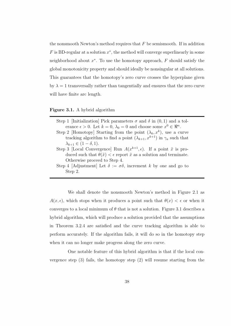
Figure 3.1. A hybrid algorithm

Step 1 [Initialization] Pick parameters σ and δ in (0, 1) and a tol-erance ε > 0. Let k = 0, λ0 = 0 and choose some x0 ∈ <n.

Step 2 [Homotopy] Starting from the point (λk, xk), use a curve

tracking algorithm to find a point (λk+1, xk+1) in γa such that

λk+1 ∈ (1− δ, 1).Step 3 [Local Convergence] Run A(xk+1, ε). If a point x is pro-

duced such that θ(x) < ε report x as a solution and terminate.Otherwise proceed to Step 4.

Step 4 [Adjustment] Let δ := σδ, increment k by one and go toStep 2.

We shall denote the nonsmooth Newton’s method in Figure 2.1 as

A(x, ε), which stops when it produces a point such that θ(x) < ε or when it

converges to a local minimum of θ that is not a solution. Figure 3.1 describes a

hybrid algorithm, which will produce a solution provided that the assumptions

in Theorem 3.2.4 are satisfied and the curve tracking algorithm is able to

perform accurately. If the algorithm fails, it will do so in the homotopy step

when it can no longer make progress along the zero curve.

One notable feature of this hybrid algorithm is that if the local con-

vergence step (3) fails, the homotopy step (2) will resume starting from the

38

last point found on γa. This contrasts the algorithm in [1] and is motivated

by the fact that when Newton’s method stalls, it usually gets stuck in a local

minimum of the merit function, which may cause the homotopy method to

perform poorly.

3.4 Solving Mixed Complementarity Problems

When all bounds are finite, the reformulation of the Mixed Comple-

mentarity Problem into a zero finding problem by the nonsmooth operator H

presented in (2.12) and its smoother Hµ in (2.26) are particularly well suited

for use with the algorithm in this chapter. If all bounds are finite on the MCP

that defines H, all of the conditions for convergence are automatically satis-

fied except for (3.3), which can be met by choosing a smoother that closely

approximates H. If in addition H is BD-regular at all solutions, the Newton

component of the hybrid algorithm will converge superlinearly.

To use this algorithm to solve the problem MCP(F,Bl,u), by solving

the equation H(x) = 0, it only remains to show how to generate elements

of the subdifferential ∂BH(x) to be used in the nonsmooth Newton’s method

presented in Figure 2.1. Such a procedure is provided in Figure 3.2. In [1] it

is proved that this procedure will produce an element of ∂BH(x). Since we

are using this procedure only in Newton’s method to solve H(x) = 0, we may

consider just the case when µ = 0 in this procedure.

39

Figure 3.2. Procedure to evaluate an element of ∂BH(x)

Step 1 Set βl := { i | xi − li = 0 = Fi(x)} andβu := { i | ui − xi = 0 = Fi(x)}

Step 2 Choose z ∈ <n such that zi 6= 0 for all i ∈ βl⋃βu.

Step 3 For each i, if i 6∈ βu, or µ 6= 0, set

ci(x) :=xi − ui√

(xi − ui)2 + Fi(x)2 + 2µ+ 1

di(x) :=Fi(x)√

(xi − ui)2 + Fi(x)2 + 2µ+ 1;

else if µ = 0 and i ∈ βu, set

ci(x) :=zi

‖(zi,∇Fi(x)z)‖+ 1

di(x) :=∇Fi(x)z

‖(zi,∇Fi(x)z)‖+ 1.

Step 4 For each i, if i 6∈ βl or µ 6= 0, set

ai(x) := 1− xi − li√(xi − li)2 + φ(ui − xi,−Fi(x))2 + 2µ

bi(x) := 1− φ(ui − xi,−Fi(x))√(xi − li)2 + φ(ui − xi,−Fi(x))2 + 2µ

;

else if µ = 0 and i ∈ βl, set

ai(x) := 1− zi‖(zi, ci(x)zi + di(x)∇Fi(x)z)‖

bi(x) := 1− ci(x)zi + di(x)∇Fi(x)z)

‖(zi, ci(x)zi + di(x)∇Fi(x)z)‖.

Step 5 For each i, set

Vi := (ai(x) + bi(x)ci(x))ei>

+ bi(x)di(x)∇Fi(x).

40

4. Implementation

4.1 HOMTOOLS

The algorithm described in the previous chapter is but one of many

possible approaches for using homotopy-based techniques to solve nonsmooth

equations. Our ultimate interest lies in exploring variants of this algorithm.

To aid in the development of such algorithms, this thesis develops a suite of

MATLAB routines called HOMTOOLS, which allows algorithm developers to

prototype and evaluate homotopy-based solvers in a MATLAB environment.

HOMTOOLS provides a uniform interface by which clients can request a prob-

lem to be solved, and several convenience routines to aid in the construction

of solvers. Some of these routines are MATLAB Mex interfaces into routines

from HOMPACK90, which allow developers to build solvers from highly so-

phisticated atomic routines. For the client, HOMTOOLS provides an interface

to the MCPLIB library of complementarity problems, which serves as a conve-

nient test library for the solvers. Table 4.2 outlines the basic structure of the

six packages of the HOMTOOLS interface. The prefixes on the functions have

been omitted for ease of reading.

The Root Finding package provides clients a way to specify the ho-

motopy map and solver to be used and provides a uniform interface through

which users may invoke the specified solver. It provides solvers the ability to

recover functions implementing the homotopy map.

The Homotopy Smooth package creates the homotopy map defined in

(3.2) on a function and its smoother and initializes the Root Finding package.

41

The Utility package provides functions that can be used to reformulate

Mixed Complementarity Problems as specified in Section 2.4.

The MCP Smooth package uses the Utility package to construct the

function H and its smoother Hµ described in Section 2.7.1 given an MCP

defined by a function and upper and lower bound vectors. This package uses

these functions to initialize the Homotopy Smooth package.

The GAMS MCP package interfaces with GAMS [8] to make avail-

able problems from MCPLIB, a large test library of complementarity problems

defined in GAMS. It obtains handles to functions and bound vectors which

are used to initialize the MCP Smooth package. This package allows problems

from MCPLIB to be solved simply by specifying the model name and a starting

point.

The Algorithms package contains convenience routines to help deve-

lopers build solvers. Some of these routines are Mex interfaces into the HOM-

PACK90 suite of codes.

A more detailed description of HOMTOOLS with examples follows.

In order to function as a homotopy-based solver for the equation

F (x) = 0, (4.1)

a routine must be provided with functions to evaluate a homotopy mapping

and its Jacobian:

ρa(λ, x) and (4.2)

∇ρa(λ, x). (4.3)

The functions F (x) and ∇F (x) may be evaluated by taking ρa(1, x) and

∇ρa(1, x) respectively, however for convenience and efficiency the solver should

be able to evaluate these functions directly, especially if F is nonsmooth. To

42

be as general as possible, the solver routine should be provided with an open

set of parameters. We will assume that solvers used with HOMTOOLS have

the following MATLAB function signature:

[x njac arclen status] = solverName(n,x0,A,

arcre,arcae,ansre,ansae,maxnfe,sspar)(4.4)

where the parameters are defined in Table 4.1.

The remainder of this section describes each package of HOMTOOLS

in detail and presents some examples of how to use each package. These pack-

ages are presented so that each package directly depends and builds on the

previous one excepting the Utility package, which is independent of the rest

of HOMTOOLS and the Algorithms package, which only depends on the Root

Finding package. One should also note that the packages in HOMTOOLS

were designed so that they depend on one another through interface only. If

any package’s implementation is unsatisfactory for a particular application, it

may be replaced with a different package that offers the same function names,

signatures, and semantics.

4.1.1 The Root Finding Package. At the base of the HOM-

TOOLS suite is a package called Root Finding. This package is responsible

for associating a user-specified solver with MATLAB functions implementing

(4.2) and (4.3) and providing a uniform interface by which clients may solve

equations. The core set of functions in the Root Finding package follow.

H initRootFinding(fName,fjacName,rhoName,rhojacName) (4.5)

This function takes as input the names of MATLAB routines that can be used

to evaluate F , ρa, and their Jacobians. These arguments are passed in as single

quoted strings so that they may later be invoked through a call to the feval()

43

Table 4.1. Parameters for a HOMTOOLS compliant solver

Input:n problem sizex0 starting pointA parameter in (4.2)arcre relative error for curve trackingarcae absolute error for curve trackingansre relative error for end gameansae absolute error for end gamemaxnfe maximum number of Jacobian evaluations to be performedsspar any MATLAB object - defaults to HOMPACK90 conventionsOutput:x alleged answernjac number of Jacobian evaluations performedarclen approximate length of the homotopy curve that was trackedstatus solver dependent error flag

44

Table 4.2. Overview of the HOMTOOLS public interface

Package FunctionRoot Finding initRootFinding()

setImpl()findRoot()getDefaultArgs()getArgs()setArgs()merit()F() Fjac() rho() rhojac()

Homotopy Smooth initHomotopySmooth()util mu() mujac()

phi() phijac()psi() psijac()Alpha()

MCP Smooth initMCPSmooth()solveMCP()testSoln()

GAMS MCP solveGamsMCP()Algorithms fixpnf() - from HOMPACK90

stepnf() - from HOMPACK90

45

function in MATLAB. The necessary signatures of these routines are the same

as those in (4.6) – (4.9).

y = Hrf F(x) (4.6)

dy = Hrf Fjac(x) (4.7)

z = Hrf rho(lambda,x) (4.8)

dz = Hrf rhojac(lambda,x) (4.9)

In these routines, dy and dz are Jacobian matrices of dimensions n × n and

n× (n+ 1) respectively.

Hrf setImpl(solverName) (4.10)

This function takes as input the name of a MATLAB routine as a single quoted

string. The function specified by solverName must have a calling signature

identical to (4.4).

[x njac arclen status] = H findRoot(n,x0,A,

arcre,arcae,ansre,ansae,maxnfe,sspar)(4.11)

This function invokes the specified solver and returns the results. A call can be

made to H findRoot() only after Hrf initRootFinding() and

Hrf setImpl() are called. The parameters in this function have the same

meanings as in (4.4). The first three parameters are mandatory and the

remaining arguments have defaults that can be specified through a call to

Hrf setArgs() and recovered through a call to Hrf getArgs(). These func-

tions simply allow the user to specify and the solver to recover the parameters

arcre, arcae, ansre, ansae, maxnfe, and sspar.

Hrf setArgs(arcre,arcae,ansre,ansae,maxnfe,sspar) (4.12)

46

[arcre,arcae,ansre,ansae,maxnfe,sspar] = Hrf getArgs() (4.13)

Example 4.1.1 Suppose we have written a MATLAB function with the same

signature as (4.4) called mySolver and routines myF, myFJac, myRho, and

myRhoJac with signatures corresponding to (4.6) – (4.9). To initialize the

Root Finding package the following code may be executed.

Hrf_setImpl(’mySolver’);

H_initRootFinding(’myF’,’myFJac’,’myRho’,’myRhoJac’);

These calls associate the MATLAB functions implementing F and ρa with

the solver whose implementation is contained in the MATLAB function called

mySolver. The solver has visibility to the functions Hrf F, Hrf FJac, Hrf rho,

and Hrf rhojac in the Root Finding package. These routines have the same

signature as the respective arguments passed into (4.5), and calls to them will

result in the invocation of those functions passed into H initRootFinding().

A client may then invoke the solver with a call to

[x njac arclen status] = H_findRoot(length(x),x,A);

which uses default arguments, or by the extended form:

[x njac arclen status] = H_findRoot(n,x0,A,

arcre,arcae,ansre,ansae,maxnfe,sspar);

The advantage of the approach taken in this package is that it de-

couples the code implementing the solver from the code that uses it. The

solver must only be aware of the interfaces to the functions in the Root Find-

ing package, while clients are free to vary the implementation and names of

the functions invoked by this package. This type of decoupling is a dominant

theme in the design of HOMTOOLS.

47

Passing the names of functions in this manner is meant to simulate

the use of function pointers that are available in a language such as C. Unfortu-

nately this practice is more hazardous in the MATLAB environment because

it lacks compiler type safety and a namespacing or scoping mechanism. An

incorrect calling sequence will, in most cases, produce a meaningful runtime

error, however.

4.1.2 The Utility Package. The utility package contains rou-

tines that are used by the remaining sections. They are germane to the reformu-

lation of a complementarity problem into a parameterized smoother Hµ(λ)(x)

(2.26) for H(x) (2.12) as discussed in Section 2.7. It contains the following

routines.

mu = Hutil mu(lambda) (4.14)

dmu = Hutil muJac(lambda) (4.15)

alpha = Hutil Alpha(alpha) (4.16)

p = Hutil phi(mu,a,b) (4.17)

dp = Hutil phijac(mu,a,b) (4.18)

p = Hutil psi(mu,l,u,x,f) (4.19)

dp = Hutil psijac(mu,l,u,x,f) (4.20)

Currently this package implements Hutil mu as

µα(λ) := α(1− λ)2

where the parameter α is obtained through a call to Hutil Alpha(), which

may be specified by the user. If an argument is provided to Hutil Alpha()

the package takes that to be the current α. If no argument is provided the

function simply returns the current value of α.

48

Hutil phi is implemented as the smoother for the Fischer-Burmeister

function (2.24)

φµ(a, b) := a+ b−√a2 + b2 + 2µ.

The Hutil psi routine implements the Kanzow MCP smoother (2.25) as

ψµ(l, u, x, f) := φµ(x− l,−φµ(u− x,−f)).

The implementation of these functions is particular to a specific refor-

mulation of the Mixed Complementarity Problem. If these functions are not

suitable for a particular reformulation they may be replaced with functions,

which have more appropriate implementations. For example, the component-

wise median function is a valid NCP function (see Definition 2.4.1), so any im-

plementation of a smoother for that function may be substituted for Hutil phi

and Hutil phijac.

4.1.3 The Homotopy Smooth Package. Although the Root Find-

ing package may be used directly, clients must supply it with meaningful ho-

motopies. The Homotopy Smooth package is used to create those homotopies

for nonsmooth systems that we are considering in this thesis. To do this it uses

the homotopy map presented in Chapter 3

ρa(λ, x) := λF µα(λ)(x) + (1− λ)(x− a) (4.21)

where the smoothing parameter is governed by

µα := α(1− λ)2,

which is implemented by the Hutil mu() (4.14) function in the Utility package.

Here it is assumed that F has a valid smoother F ν .

49

To construct a function implementing the homotopy mapping, the

package must be provided with routines to evaluate F , ∇F , and their associ-

ated smoothers F ν and ∇F ν . This is accomplished by initializing the package

through a call to

H initHomotopySmooth(FName,FJacName,F muName,FJac muName) (4.22)

where FName and FJacName are the single quoted string names of MATLAB

functions implementing F and ∇F , and F muName and FJac muName represent

their smoothers. This call provides the following functions with the implemen-

tations provided as inputs. For example, a call to Hhs F will result in a call to

the function specified in the above FName parameter.

y = Hhs F(x) (4.23)

dy = Hhs FJac(x,k) (4.24)

y = Hhs rho(lambda,x) (4.25)

dy = Hhs rhojac(lambda,x,k) (4.26)

Here dy is an n×nmatrix. The call to H initHomotopySmooth() also initializes

the Root Finding package by calling H initRootFinding() and passing in the

function names of (4.23) – (4.26) as arguments, thus providing a homotopy

mapping for dealing with nonsmooth systems. Because the function F need

not be smooth, the function Hhs FJac is required to return an element of the

B-subdifferential of F .

4.1.4 The MCP Smooth Package. The purpose of the MCP

Smooth package is to reformulate an MCP into a system of equations using a

smoothed version of the reformulation presented in Section 2.4. To reformulate

50

the problem MCP(F,Bl,u) (Section 2.3) this package needs to be provided with

MATLAB functions through a call to

H initMCPSmooth(FName,FJacName) (4.27)

where FName and FJacName are the names of MATLAB functions implement-

ing F and its Jacobian ∇F . This function initializes the Homotopy Smooth

package with a call to H initHomotopySmooth() with the following functions

as arguments.

y = Hmcp H(x) (4.28)

dy = Hmcp HJac(x) (4.29)

y = Hmcp H mu(x) (4.30)

dy = Hmcp HJac mu(x) (4.31)

To solve an MCP, simply initialize the package and invoke the function

[z njac arclen status] = H solveMCP(z0,l,u) (4.32)

where z0 is a starting point for the problem and l and u are the vectors of

lower and upper bounds that define the box Bl,u. The output parameters are

identical to those in (4.11).

Since the stopping criteria for the algorithm is solver dependent, an

independent check for solution quality is necessary. This is provided by the

function

residual = Hmcp testSoln(z) (4.33)

which must be invoked after the problem has been initialized and run. Since

z solves MCP(F,Bl,u) if and only if mid(x − l, x − u, F (x)) = 0, the residual

vector r is computed as

r = |mid(x− l, x− u, F (x))|

51

where | · | is the componentwise absolute value function. The output parameter

residual should be nearly zero in every component if a solution to the problem

defined by previous calls to H initMCPSmooth() and H solveMCP() is given as

an input argument.

4.1.5 The GAMS MCP Package. The GAMS MCP package is

a special extension to MCP Smooth, which allows a complementarity problem

to be specified in GAMS and imported into and solved in MATLAB. This

package is implemented using a GAMS to MATLAB interface presented in [8].

It allows developers to test solvers against entire libraries of complementarity

problems specified in the GAMS environment [2].

The GAMS MCP package offers clients only one function:

[z njac arclen status] = H solveGamsMCP(num,literal,name).

(4.34)

The input parameter name is a single quoted string containing the name of a

GAMS model. The num parameter is an integer specifying the point at which

point to start; this point is provided by the GAMS to MATLAB interface de-

scribed in [8]. Alternatively, one could pass in a vector into the num parameter.

If it is of correct dimension and the literal argument is not zero, the routine

will use it as a starting point for the MCP. The output parameters have the

same meanings as in (4.11).

Example 4.1.2 A typical case that illustrates how to use the GAMS MCP

package with HOMTOOLS follows.

Hrf_setImpl(’H_hompack’);

Hutil_Alpha(0.8);

Hrf_setArgs(10e-2,10e-2,10e-12,10e-12,1000,20.0,[0 0 0 0 0 0 0 0]’);

[z njac arclen status] = H_solveGamsMCP(2,0,’josephy’);

52

residual = Hmcp_testSoln(z);

This MATLAB program will attempt to solve the josephy model from the

MCPLIB library using a solver called H hompack and report if the problem was

solved. The client need only specify which solver to use and which problem

to solve. The other calls serve to customize the solver. This customization is

not strictly necessary as the parameters have reasonable defaults; however, it

is usually desirable to do so.

4.1.6 The Algorithms Package. This package currently con-

tains two routines exported from HOMPACK90. The H fixpnf() algorithm is

a Mex interface to the routine described in detail in Section 2.6.2. It has the

following interface.

[z njac arclen iflag] = H fixpnf(n,x0,A,

arcre,arcae,ansre,ansae,iflag,sspar);(4.35)

The H stepnf() routine generates the iterates inside the H fixpnf() routine.

It has the following signature.

[y yp yold ypold h hold njac arclen iflag] =

H stepnf(n,A,y,yp,ypold,abserr,relerr,iflag,start)(4.36)

This function takes y to be the current point on the zero curve and yp to be

the associate tangent vector. ypold is a tangent vector to which yp must be

acute. The abserr and relerr parameters are used to detect convergence in

the corrector phase of the algorithm. The start parameter should be set to

1 the first time the routine is called. iflag is an error status documented

in HOMPACK90. It should be -2 on input and 0 on output. Should iflag

return greater than 0, then the algorithm has failed and iflag is an error code

documented in the HOMPACK90 source code.

53

4.2 Solver Implementation

To implement the hybrid algorithm presented in Figure 3.1, we used

HOMTOOLS in the MATLAB environment. The nonsmooth Newton’s method

used for local convergence in Step 3 of the algorithm is a straight-forward

implementation of the algorithm presented in Figure 2.1.

To implement Step 2 of the hybrid algorithm, we use a routine similar

to HOMPACK90’s FIXPNF (see Section 2.6.2) to track the zero curve of the

homotopy map. This routine is a MATLAB function that uses a MEX interface

to the STEPNF routine from HOMPACK90 to generate iterates along the zero

curve. Its implementation differs from FIXPNF’s in that it omits the end game

strategy. The routine takes an input parameter δ ∈ (0, 1) so that as soon as it

produces a point (λ, x) on the zero curve with λ ∈ (1− δ, 1) it returns and lets

the Newton method take care of the end game convergence. If the STEPNF

routine produces an iterate such that its λ component is greater than one,

the algorithm simply throws away the point and calls STEPNF again with the

maximum allowable stepsize reduced by some prescribed factor (default is 0.5).

As with the end game strategy, our curve tracking algorithm differs

from the FIXPNF routine in that it uses a different heuristic to control how

tightly the iterates follow the zero curve when it detects that the curve is par-

ticularly nonlinear. Assume that the previous iterate on the zero curve we have

accepted is (λ0, x0) and that the STEPNF routine indicates that (λ, x) should

be the next. This algorithm will accept this point as the next iterate provided

that the angle between (λ0, x0) and (λ, x) is smaller that some prescribed angle

(it defaults to 60 degrees). This strategy is intended to ensure that the iterates

follow the zero curve more closely when the curve is highly nonlinear. The

intent is to prevent the algorithm from producing a point that is on a different

54

component of %−1a ({0}) and to make sure that it does not start tracking the

curve in the wrong direction of the correct component.

To solve complementarity problems, we used the MATLAB to GAMS

interface described in [8]. This interface allows one to specify an MCP in the

GAMS environment and obtain the bounds and evaluate the function and

associated Jacobian that define the MCP from the MATLAB environment.

These functions and bounds are accessed through the GAMS MCP package in

HOMTOOLS. The function implementing our hybrid algorithm is passed into

the Hrf setImpl() function in the Root Finding package.

55

5. Results and Conclusions

To test the performance of the algorithm presented in Chapter 3 we

used the implementation discussed in Section 4.2 along with the FIXPNF rou-

tine from HOMPACK90 on the MCPLIB, a set of Mixed Complementarity

Problems specified in the GAMS language. The performance of several com-

plementarity solvers has been tested and documented against this library [2].

Because the HOMTOOLS package can incur a large overhead and currently

only supports the use of dense Jacobians, we tested the algorithm on all prob-

lems in the MCPLIB having fewer than 100 variables at all starting points

provided by the GAMS to MATLAB interface in [8].

5.1 Testing Procedure

For initial testing, we chose a set of default parameters to use in the

hybrid algorithm, which takes as input the same arguments as the FIXPNF

routine described in Section 2.6.2 as well as those specified in Step 1 of the

algorithm in Figure 3.1. For the curve tracking tolerance parameters we chose

values of arcae = arcre = 10−2. These loose curve tracking parameters were

chosen so that reasonable progress would be made along the homotopy’s zero

curve. The answer tolerances ε, ansae, and ansre were chosen to be 10−10.

The sspar parameters from FIXPNF (also used in STEPNF, described in Sec-

tion 2.6.2) are taken as their default values in HOMPACK90.

We tested the method in three ways. First as a generalized Newton’s

method. The δ parameter is chosen to be 1.0 on initialization. This causes

the Newton method to be executed before the homotopy phase during the first

56

Table 5.1. MCPLIB Test Problems

δ = 1 δ = 0.01 FIXPNFProblem st. Step 2 Jac Step 2 Jac JacName pt. size calls evals calls evals evalsbadfree 1 5 4 22 1 18 failbertsekas 1 15 7 424 3 382 failbertsekas 2 15 7 562 3 526 777bertsekas 3 15 12 fail 3 627 809billups 1 1 1 13 1 18 14box 1 44 1 fail 1 fail failcolvdual 1 20 1 53 1 83 88colvdual 2 20 1 58 1 66 109colvnlp 1 15 1 61 1 83 89colvnlp 2 15 0 10 1 48 53colvtemp 1 20 1 53 1 83 88degen 1 2 0 5 1 12 14ehl k40 1 41 1 110 1 128 134ehl k60 1 61 1 fail 1 fail failehl k80 1 81 1 428 1 432 failexplcp 1 16 0 5 1 24 18freebert 1 15 7 614 3 608 failfreebert 2 15 0 10 1 fail failfreebert 3 15 7 253 3 295 failfreebert 4 15 7 582 3 577 failfreebert 5 15 0 13 2 fail failfreebert 6 15 7 433 3 433 541gafni 1 5 0 13 1 44 42gafni 2 5 0 11 1 128 60gafni 3 5 0 12 1 fail 98games 1 16 0 32 4 fail failhanskoop 1 14 2 36 1 41 36hanskoop 2 14 1 28 1 39 42hanskoop 3 14 1 23 1 32 31hanskoop 4 14 1 26 1 34 33hanskoop 5 14 2 87 1 176 failhydroc06 1 29 0 5 1 fail fail

57

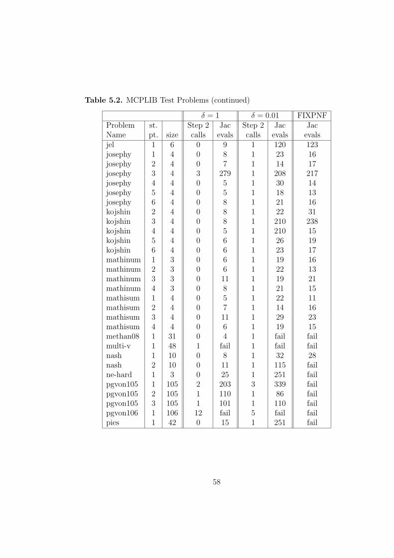
Table 5.2. MCPLIB Test Problems (continued)

δ = 1 δ = 0.01 FIXPNFProblem st. Step 2 Jac Step 2 Jac JacName pt. size calls evals calls evals evalsjel 1 6 0 9 1 120 123josephy 1 4 0 8 1 23 16josephy 2 4 0 7 1 14 17josephy 3 4 3 279 1 208 217josephy 4 4 0 5 1 30 14josephy 5 4 0 5 1 18 13josephy 6 4 0 8 1 21 16kojshin 2 4 0 8 1 22 31kojshin 3 4 0 8 1 210 238kojshin 4 4 0 5 1 210 15kojshin 5 4 0 6 1 26 19kojshin 6 4 0 6 1 23 17mathinum 1 3 0 6 1 19 16mathinum 2 3 0 6 1 22 13mathinum 3 3 0 11 1 19 21mathinum 4 3 0 8 1 21 15mathisum 1 4 0 5 1 22 11mathisum 2 4 0 7 1 14 16mathisum 3 4 0 11 1 29 23mathisum 4 4 0 6 1 19 15methan08 1 31 0 4 1 fail failmulti-v 1 48 1 fail 1 fail failnash 1 10 0 8 1 32 28nash 2 10 0 11 1 115 failne-hard 1 3 0 25 1 251 failpgvon105 1 105 2 203 3 339 failpgvon105 2 105 1 110 1 86 failpgvon105 3 105 1 101 1 110 failpgvon106 1 106 12 fail 5 fail failpies 1 42 0 15 1 251 fail

58

Table 5.3. MCPLIB Test Problems (continued)

δ = 1 δ = 0.01 FIXPNFProblem st. Step 2 Jac Step 2 Jac JacName pt. size calls evals calls evals evalspowell 1 16 0 9 2 99 57powell 2 16 0 12 1 fail failpowell 3 16 1 242 1 265 failpowell 4 16 0 12 1 62 226powell mcp 1 8 0 6 1 24 22powell mcp 2 8 0 7 1 26 25powell mcp 3 8 0 9 1 42 45powell mcp 4 8 0 8 1 29 28qp 1 4 0 2 1 16 13scarbsum 1 40 3 fail 1 fail failscarfanum 1 13 1 39 1 37 failscarfanum 2 13 0 13 1 39 38scarfanum 3 13 0 12 3 69 failscarfasum 1 14 0 9 1 fail failscarfasum 2 14 1 100 1 fail failscarfasum 3 14 1 64 1 fail failscarfbnum 1 39 12 589 5 224 failscarfbnum 2 39 10 523 5 224 failscarfbsum 1 40 1 74 2 234 failscarfbsum 2 40 7 273 3 183 failshubik 1 42 20 fail 11 fail failsimple-ex 1 17 1 42 1 39 40simple-red 1 13 0 11 1 30 31sppe 1 27 1 69 1 114 failsppe 2 46 1 46 3 87 failtobin 1 7 1 82 1 82 83tobin 2 7 0 9 1 79 78

59

time through the hybrid algorithm. If the Newton method solves the problem,

the homotopy method is never invoked. The δ-reduction factor σ was chosen to

be 0.5. The second configuration used the same hybrid algorithm, except with

the initial δ = 0.01. This causes the homotopy method to do most of the actual

work, using Newton’s method only for the ‘end game’ phase. If no solution

was produced within 30 iterations of the hybrid method the algorithm was

terminated. If Step 3 produced more than 1000 points on the homotopy curve

without returning that phase was terminated. Finally, we ran the problem set

with the FIXPNF routine from HOMPACK, including the standard ‘end game’

strategy from FIXPNF.

5.2 Computational Results

Using a single set of parameters the implementation of the algorithm

described in Chapter 3 was able to solve many problems on which Newton’s

method alone failed. There were also some problems that Newton’s method

solved and the hybrid algorithm could not solve by using the homotopy method.

The FIXPNF routine failed on many problems. This is can be attributed to

the fact that the standard ‘end game’ strategy of FIXPNF was not designed

to handle nonsmooth functions.

5.3 Conclusions

While this algorithm solved most of the test problems, compared to

other complementarity solvers [2] its current implementation is very slow in

terms of the number of Jacobian evaluations required to produce a solution.

A degree of slowness is characteristic of homotopy based algorithms, however,

what they lack in speed they tend to make up for in robustness. The theoretical

foundation presented in Chapter 3 almost surely (in the sense of Lesbegue

60

measure), under very weak assumptions, guarantees the existence of a zero

curve that can be tracked to a solution. This theoretical foundation ensures

that any algorithm that can accurately track the zero curve will converge to a

solution.

In spite of the solid theory supporting the algorithm, this method

failed altogether on a number of problems and required carefully chosen pa-

rameters to solve several others. For some of these problems, the failure was

due to the fact that the Jacobian of the problem’s reformulation was singular at

the solution. In this case the theory suggests the algorithm could fail because

the zero curve of the homotopy map may have infinite arc length.

The homotopy-based approach for solving nonsmooth systems pre-

sented in this paper is neither extremely robust nor efficient in its current

implementation. It does, however, bring to bear some powerful theory, which

suggests that it should be very robust for a large class of problems. It remains

to determine exactly why the algorithm performs poorly or fails altogether on

many problems. The poor performance might be due to the difficulty of ac-

curately tracking the homotopy curves or it could be that some problems are

violating a theoretical requirement.

5.4 Avenues for Further Research

At present this algorithm could be used in cases where more conven-

tional methods fail. To improve the robustness and performance of the algo-

rithm, there are two approaches that can be taken: develop homotopy maps

that induce a more well-behaved zero curve, or develop a better approach for

tracking the curve induced by the map presented in Chapter 3. One way to

accomplish the latter task might be to develop a new curve tracking paradigm

whereby the zero curve is tracked with increasing tolerance as progress is made

61

along it. This contrasts the approach presented in HOMPACK90’s FIXPNF

algorithm, which tracks the zero curve with a uniform tolerance all the way

until the end game phase. Such an approach may be more efficient because

the algorithm can take longer steps along the zero curve during the beginning

of the algorithm and may be able to make good progress even when the zero

curve has sharp turns. This approach may also dove-tail more elegantly into

the end game phase of the algorithm since the curve tracking tolerance shrinks

as it approached a solution.

62

REFERENCES

[1] S. C. Billups. A homotopy based algorithm for mixed complementari-ty problems. UCD/CCM Report No. 124, Department of Mathematics,University of Colorado at Denver, Denver, Colorado, 1998.

[2] S. C. Billups, S. P. Dirkse, and M. C. Ferris. A comparison of large scalemixed complementarity problem solvers. Computational Optimization andApplications, 7:3–25, 1997.

[3] C. Buck. Advanced Calculus. McGraw–Hill, New York, NY, 3rd edition,1978.

[4] B. Chen and X. Chen. A global linear and local quadratic continuationsmoothing method for variational inequalities with box constraints. AM-R 96/39, School of Mathematics, The University of New South Wales,Sydney, Australia, 1997.

[5] S. N. Chow, J. Mallet-Parret, and J. A. Yorke. Finding zeroes of maps:Homotopy methods that are constructive with probability one. Mathe-matics of Computing, 32:887–899, 1978.

[6] F. H. Clarke. Optimization and Nonsmooth Analysis. John Wiley & Sons,New York, 1983.

[7] J. E. Dennis and R. B. Schnabel. Numerical Methods for UnconstrainedOptimization and Nonlinear Equations. Prentice-Hall, Inc, EnglewoodCliffs, New Jersey, 1983.

[8] M. C. Ferris and T. F. Rutherford. Accessing realistic complementarityproblems within Matlab. In G. Di Pillo and F. Giannessi, editors, Non-linear Optimization and Applications, pages 141–153. Plenum Press, NewYork, NY, 1996.

[9] A. Fischer. A special Newton–type optimization method. Optimization,24:269–284, 1992.

63

[10] A. Fischer. An NCP–function and its use for the solution of complemen-tarity problems. In D. Z. Du, L. Qi, and R. S. Womersley, editors, Re-cent Advances in Nonsmooth Optimization, pages 88–105. World ScientificPublishers, 1995.

[11] G. H. Golub and C. F. Van Loan. Matrix Computations. The JohnsHopkins University Press, Baltimore, Maryland, 1983.

[12] P. T. Harker and J.-S. Pang. Finite–dimensional variational inequalityand nonlinear complementarity problems: A survey of theory, algorithmsand applications. Mathematical Programming, 48:161–220, 1990.

[13] C. Kanzow. Some equation–based methods for the nonlinear complemen-tarity problem. Optimization Methods and Software, 3:327–340, 1994.

[14] D. MacMillan. Relaxing Convergence Conditions to Improve the Conver-gence Rate. PhD thesis, University of Colorado at Denver, Denver, CO,April 1999.

[15] L. W. McKenzie. General equlibrium. In J. Eatwell, editor, The NewPalgrave: A Dictionary of Economics, volume 2. MacMillan Press Ltd.,Oxford, England, 1987.

[16] J.-S. Pang and L. Qi. Nonsmooth equations: Motivation and algorithms.SIAM Journal on Optimization, 3:443–465, 1993.

[17] L. Qi and J. Sun. A nonsmooth version of Newton’s method. Mathemat-ical Programming, 58:353–368, 1993.

[18] H. E. Scarf. The Computation of Economic Equilibria. Yale UniversityPress, New Haven, Connecticut, 1973.

[19] H. R. Varian. Microeconomic Analysis. W.W. Norton & Company, NewYork, New York, 1978.

[20] L. T. Watson. An algorithm that is globally convergent with probabilityone for a class of nonlinear two-point boundary value problems. SIAMJournal on Numerical Analysis, 16:394–401, 1979.

[21] L. T. Watson. Solving the nonlinear complementarity problem by a ho-motopy method. SIAM Journal on Control and Optimization, 17:36–46,1979.

64

[22] L. T. Watson, S. C. Billups, and A. P. Morgan. Algorithm 652: HOM-PACK: A suite of codes for globally convergent homotopy algorithms.ACM Transactions On Mathematical Software, 13:281–310, 1987.

[23] L. T. Watson, R. C. Melville, A. P. Morgan, and H. F. Walker. Algorithm777: HOMPACK90: A suite of Fortran 90 codes for globally convergen-t homotopy algorithms. ACM Transactions On Mathematical Software,23:514–549, 1997.

65