6 May/June 2013 Published by the IEEE Computer Society 0272-1716/13/$31.00 © 2013 IEEE

Visualization Viewpoints Editor: Theresa-Marie Rhyne

Using GPU Shaders for Visualization, Part 3Mike BaileyOregon State University

GPU shaders aren’t just for glossy special effects. Parts 1 and 2 of this discussion looked at using them for point clouds,

cutting planes, line integral convolution, and terrain bump-mapping.1,2 Here, I cover compute shaders and shader storage buffer objects (SSBOs), which are new features of OpenGL (Open Graph-ics Library).

Originally, OpenGL was for graphics only. But practitioners soon gazed longingly at the GPU’s power and wanted to use it for nongraphics data-parallel computing. This led to the general-purpose GPU (GPGPU) approach.3 This approach was quite effective and produced some amazing results. However, it was still an awkward workaround that required fi rst recasting the data-parallel problem as a pixel-parallel problem.

True mainstream GPGPU emerged with Nvidia’s CUDA (Compute Unifi ed Device Architecture).4

CUDA treats the GPU as a real compute engine without any need to include graphics remnants. Later, OpenCL (Open Computing Language) was de-veloped to create a multivendor GPU-programming standard.5,6

OpenGL 4.3 introduced SSBOs, which support compute shaders and make getting data into and out of them much easier. This means that, fi nally, using GPUs for data-parallel visualization comput-ing is a fi rst-class feature of OpenGL. This will greatly assist real-time visualization techniques such as particle advection and isosurfaces.

Compute ShadersUsing compute shaders looks much like standard two-pass rendering (see Figure 1). The GPU gets invoked at least twice, once for the compute opera-tion and once or more for the graphics operation. The compute shader manipulates GPU-based data. The OpenGL rendering pipeline creates a scene based on those new data values.

At this point, I’ll dive down into details and as-

sume you have knowledge of OpenGL7 and GLSL (OpenGL Shading Language) shaders,8,9 including how to write, compile, and link them.

A compute shader is a single-stage GLSL pro-gram that has no direct role in the graphics ren-dering pipeline. It sits outside the pipeline and manipulates data it fi nds in the OpenGL buffers. Except for a handful of dedicated built-in GLSL variables, compute shaders look identical to all other GLSL shader types. The programming syn-tax is the same. They access the same data that’s found in the OpenGL readable data types, such as textures, buffers, image textures, and atomic coun-ters. They output the same OpenGL writeable data types, such as some buffer types, image textures, and atomic counters. But they have no previous-pipeline-stage inputs or next-pipeline-stage outputs because to them there’s no pipeline and therefore no other stages.

A Comparison with OpenCLCompute shaders look much like OpenCL pro-grams. Both manipulate GPU-based data in a round-robin fashion with the rendering. The pro-gramming languages look similar. (Most of the language differences are superfi cial; for example, OpenCL uses SIMD [single instruction, multiple data] variables called float[2-4], whereas GLSL uses vec[2-4].) But some important differences do exist:

■ OpenCL is its own entity. Using OpenCL re-quires a several-step setup process in the appli-cation program.

■ OpenCL requires separate drivers and libraries.■ Compute shaders use the same context as

OpenGL rendering. OpenCL requires a context switch before and after invoking its data-parallel compute functions.

■ OpenCL has more extensive computational support.

IEEE Computer Graphics and Applications 7

So, you should continue to use OpenCL for large GPU data-parallel computing applications. But for many simpler applications, compute shaders will slide more easily into your existing shader-based program.

What’s Different about Using a Compute Shader?For the most part, writing and using a compute shader looks and feels like writing and using any other GLSL shader type, with these exceptions:

■ The compute shader program must contain no other shader types.

■ When creating a compute shader, use GL_COM-PUTE_SHADER as the shader type in the glCre-ateShader( ) function call.

■ A compute shader has no concept of in or out variables.

■ A compute shader must declare the number of work items in each of its work groups in a spe-cial GLSL layout statement.

This last item is worth further discussion. GLSL 3 introduced the layout qualifier to tell the GLSL compiler and linker about the storage of your data. This qualifier has been used for such things as tell-ing geometry shaders what their input and output topology types are, what symbol table locations certain variables will occupy, and the binding points of indexed buffers. OpenGL 4.3 expanded layout’s use to declare the local data dimensions, like this:

layout( local_size_x = 128 ) in;

I look at this in more detail later.

SSBOsOften, the tricky part of using GLSL shaders for visualization is getting large amounts of data in and out of them. OpenGL has created several ways of doing this over the years, but each seems to have had something that made it cumbersome for visu-alization use. For example, textures and uniform buffer objects can only be read from, not written to. Image textures can be both read from and writ-ten to but are backed by textures, which aren’t as data-flexible as buffer objects.

In a CPU-only data-parallel application, the most convenient data structure often is an array of structures in which each array element holds one instance of all the data variables. But none of these GLSL storage methods have allowed using this fa-miliar storage scheme in shader programming.

SSBOs aim to fix all that. They cleanly map to ar-rays of structures, which makes them convenient and familiar for data-parallel computing. Rather than talk about them, it’s easiest to show their use in actual code. The following example shows a simple particle system that uses SSBOs and com-pute shaders. Figure 2 shows the CPU code for set-ting up the required position and velocity SSBOs.

There are five things to note in the code. First, generating and binding an SSBO happens the same as with any other buffer object type, except for its GL_SHADER_STORAGE_BUFFER identifier.

Second, these SSBOs are specified with NULL as the data pointer. The data could have been filled here from precreated arrays of data. However, it’s often more convenient to create the data on the fly and fill the buffers rather than allocate large arrays first. So, in this case, data values are filled a moment later using buffer mapping.

Third, the glBufferData( ) call uses the hint GL_STATIC_DRAW. The OpenGL books say to use GL_DYNAMIC_DRAW when the values in the buf-fer will be changed often. With compute shaders, that advice is incomplete. Instead, you should use GL_DYNAMIC_DRAW when the values in the buf-fer will be changed often from the CPU. When the data values will be changed from the GPU, GL_STATIC_DRAW causes them to be kept in GPU memory, which is what you want.

Fourth, the expected call to glMapBuffer( ) has been replaced with a call to glMapBuffer-Range( ). This allows a parameter specifying that the buffer will be entirely discarded and replaced, thus hinting to the driver that it should remain in the memory (GPU) where it currently lives.

Finally, the calls to glBindBufferBase( ) al-low these buffers to be indexed. This means that they’re assigned integer indices that can be refer-enced from the shader using a layout qualifier.

Application invokes OpenGL renderingthat reads the buffer data

Application invokes the compute shaderto modify the OpenGL buffer data

A shader program, with only a compute shader in it

Another shader program, with pipeline rendering in it

Figure 1. Compute shaders involve round-robin execution between the application’s compute and rendering pieces.

8 May/June 2013

Visualization Viewpoints

Figure 3 shows how the compute shader accesses the SSBOs. Here, there are three things to note. First, the shader code uses the same set of structures to access the data as the C code did, with the data types changed to match GLSL syntax.

Second, the SSBO layout statements provide the binding indices so that the shader knows which SSBO to point to.

Finally, the open brackets in the SSBO layout

statements show how the new GLSL syntax can define an array of structures. The definition can contain more items than just that open-bracketed array, but the open-bracketed item must be the final variable in the list.

Calling the Compute ShaderA compute shader is invoked from the application with this function:

#define NUM_PARTICLES 1024 * 1024 // 1M particles to move#define WORK_GROUP_SIZE 128 // # work items per work group

struct pos{ float x, y, z, w; // positions};

struct vel{ float vx, vy, vz, vw; // velocities};

// need to do this for both the position and velocity of the particles:

GLuint posSSbo;GLuint velSSbo

glGenBuffers( 1, &posSSbo);glBindBuffer( GL_SHADER_STORAGE_BUFFER, posSSbo );glBufferData( GL_SHADER_STORAGE_BUFFER, NUM_PARTICLES * sizeof(struct pos), NULL, GL_STATIC_DRAW );GLint bufMask = GL_MAP_WRITE_BIT | GL_MAP_INVALIDATE_BUFFER_BIT ; // the invalidate makes a big difference when rewritingstruct pos *points = (struct pos *) glMapBufferRange( GL_SHADER_STORAGE_BUFFER, 0, NUM_PARTICLES * sizeof(struct pos), bufMask );

for( int i = 0; i < NUM_PARTICLES; i++ ){ points[ i ].x = Ranf( XMIN, XMAX ); points[ i ].y = Ranf( YMIN, YMAX ); points[ i ].z = Ranf( ZMIN, ZMAX ); points[ i ].w = 1.;}glUnmapBuffer( GL_SHADER_STORAGE_BUFFER );

glGenBuffers( 1, &velSSbo );glBindBuffer( GL_SHADER_STORAGE_BUFFER, velSSbo );glBufferData( GL_SHADER_STORAGE_BUFFER, NUM_PARTICLES * sizeof(struct vel), NULL, GL_STATIC_DRAW );struct vel *vels = (struct vel *) glMapBufferRange( GL_SHADER_STORAGE_BUFFER, 0, NUM_PARTICLES * sizeof(struct vel), bufMask );

for( int i = 0; i < NUM_PARTICLES; i++ ){ vels[ i ].vx = Ranf( VXMIN, VXMAX ); vels[ i ].vy = Ranf( VYMIN, VYMAX ); vels[ i ].vz = Ranf( VZMIN, VZMAX ); vels[ i ].vw = 0.;}glUnmapBuffer( GL_SHADER_STORAGE_BUFFER );

glBindBufferBase( GL_SHADER_STORAGE_BUFFER, 4, posSSbo );glBindBufferBase( GL_SHADER_STORAGE_BUFFER, 5, velSSbo );

Figure 2. Allocating and filling the shader storage buffer objects. Buffers need to be allocated, sized, and filled before the compute shaders see them.

IEEE Computer Graphics and Applications 9

glDispatchCompute( numgx, numgy, numgz );

where the arguments are the number of work groups in x, y, and z, respectively. A compute shader expects you to treat your data-parallel problem as a 3D array of work groups to pro-cess. (Although, for a 2D problem, numgz will be 1, and for a 1D problem, numgx and numgy will both be 1.) Figure 4 shows the grid of work groups. Figure 5 shows the code for invoking the compute shader.

Each work group consists of some number of work items to process. The number of groups times the number of items per group gives the total number of elements to compute. How you divide your problem into work groups is up to you. However, it’s important to experiment with this because some combinations will starve the GPU processors of work to do and some combina-tions will overwhelm them. (Also, there are some OpenGL driver-imposed limits on the number of work groups and work group size.) I experimented with the local work group size for one particular application; I discuss the results later.

Compute Shader Built-In VariablesCompute shaders have several built-in read-only variables, which aren’t accessible from any other shader types:

in uvec3 gl_NumWorkGroups ;const uvec3 gl_WorkGroupSize ;in uvec3 gl_WorkGroupID ;in uvec3 gl_LocalInvocationID ;in uvec3 gl_GlobalInvocationID ;in uint gl_LocalInvocationIndex ;

gl_NumWorkGroups is the number of work groups in all three dimensions. It’s the same num-ber used in the glDispatchCompute( ) call.gl_WorkGroupSize is the size of the work

groups in all three dimensions. It’s the same num-ber used in the layout call.gl_WorkGroupID is the work group numbers

in all three dimensions that the compute shader’s current instantiation is in.gl_LocalInvocationID is where, in all three di-

mensions, the compute shader’s current instantia-tion is in its work group.gl_GlobalInvocationID is where, in all

three dimensions, the compute shader’s current instantiation is within all instantiations.gl_LocalInvocationIndex is a 1D abstrac-

tion of gl_LocalInvocationID. It allocates

#version 430 compatibility#extension GL_ARB_compute_shader : enable#extension GL_ARB_shader_storage_buffer_object : enable;

layout( std140, binding=4 ) buffer Pos { vec4 Positions[ ]; // array of vec4 structures};

layout( std140, binding=5 ) buffer Vel { vec4 Velocities[ ]; // array of vec4 structures};

layout( std140, binding=5 ) buffer Col{ vec4 Colors[ ]; // array of structures};

Figure 3. How the shader storage buffer objects look in the shader. The shader code uses the same set of structures to access the data as the C code did, with the data types changed to match GLSL (OpenGL Shading Language) syntax.

glUseProgram( MyComputeShaderProgram );glDispatchCompute( NUM_PARTICLES / WORK_GROUP_SIZE, 1, 1 );glMemoryBarrier( GL_SHADER_STORAGE_BARRIER_BIT );

…

glUseProgram( MyRenderingShaderProgram );

// render the scene

Figure 5. Invoking the compute shader. This is how the application runs the compute shader so that the buffers get changed before rendering begins.

num_groups_x

num_groups_y

num_groups_z

Figure 4. The 3D grid of work groups allows the data to be dimensioned in a way that’s convenient to the application. It’s important to experiment with dividing a problem into work groups because some combinations will starve the GPU processors of work to do and other combinations will overwhelm them.

10 May/June 2013

Visualization Viewpoints

work group shared data arrays (which I don’t cover here).

The variables have these size ranges:

0 ≤ gl_WorkGroupID ≤ gl_NumWorkGroups – 1

0 ≤ gl_LocalInvocationID ≤ gl_WorkGroupSize – 1

gl_GlobalInvocationID = gl_WorkGroupID * gl_WorkGroupSize + gl_LocalInvocationID

gl_LocalInvocationIndex = gl_LocalInvocationID.z * gl_WorkGroupSize.y * gl_WorkGroupSize.x + gl_LocalInvocationID.y * gl_WorkGroupSize.x + gl_LocalInvocationID.x

Particle System PhysicsFigure 6 shows the code to perform particle system physics for one particle. A layout statement declares the work group size to be 128 × 1 × 1. The code defines gravity (G) and the time step (DT). G is a vec3 (3D vector) so that it can be used in a single line of code to produce the particle’s next position. The code runs once for each particle. The variable gid is the global ID—that is, the particle’s number in the entire list of particles. gid indexes into the array of structures. Figure 7 shows visualization results for this code.

Particle AdvectionFigure 8 shows how to turn the particle system into a first-order visualization of particle advection, being fed by a velocity equation as a function of particle location.

Here, there are six things to notice:

■ The code uses #defines to simulate ty-pedefs. GLSL doesn’t yet support typedefs, which, I think, are necessary to enhance the code’s readability. In this case, even though both points and velocities are really vec3s, it helps the code’s readability when you can distinguish using a coordinate from using a vector.

■ As with the code for particle physics, this code runs once for each particle. Again, the variable gid is the particle’s number in the entire list of particles, and gid indexes into the array of structures.

■ The Velocity( ) function computes (vx, vy, vz) as a function of position.

■ The equation is defined for x, y, and z between –1. and 1. If a point has moved out of bounds, it’s reset to its original position.

■ The line pp = p + DT * vel; performs a first-order particle step.

■ The particle’s color is set from the three veloc-ity components, to keep track of each particle direction. You could easily color it to show other quantities.

However, most 3D flow field data isn’t given as an equation. Figure 9 shows how you would hide

layout( local_size_x = 128, local_size_y = 1, local_size_z = 1 ) in;

const vec3 G = vec3( 0., -9.8, 0. );const float DT = 0.1;…uint gid = gl_GlobalInvocationID.x; // the .y and .z are both 1vec3 p = Positions[ gid ].xyz;vec3 v = Velocities[ gid ].xyz;vec3 pp = p + v*DT + .5*DT*DT*G;vec3 vp = v + G*DT;Positions[ gid ].xyz = pp;Velocities[ gid ].xyz = vp;

Figure 6. The shader code for one particle. It runs once for each particle.

Figure 7. Visualization results for the shader code. The particle system updates at a rate of 1.3 gigaparticles per second.

IEEE Computer Graphics and Applications 11

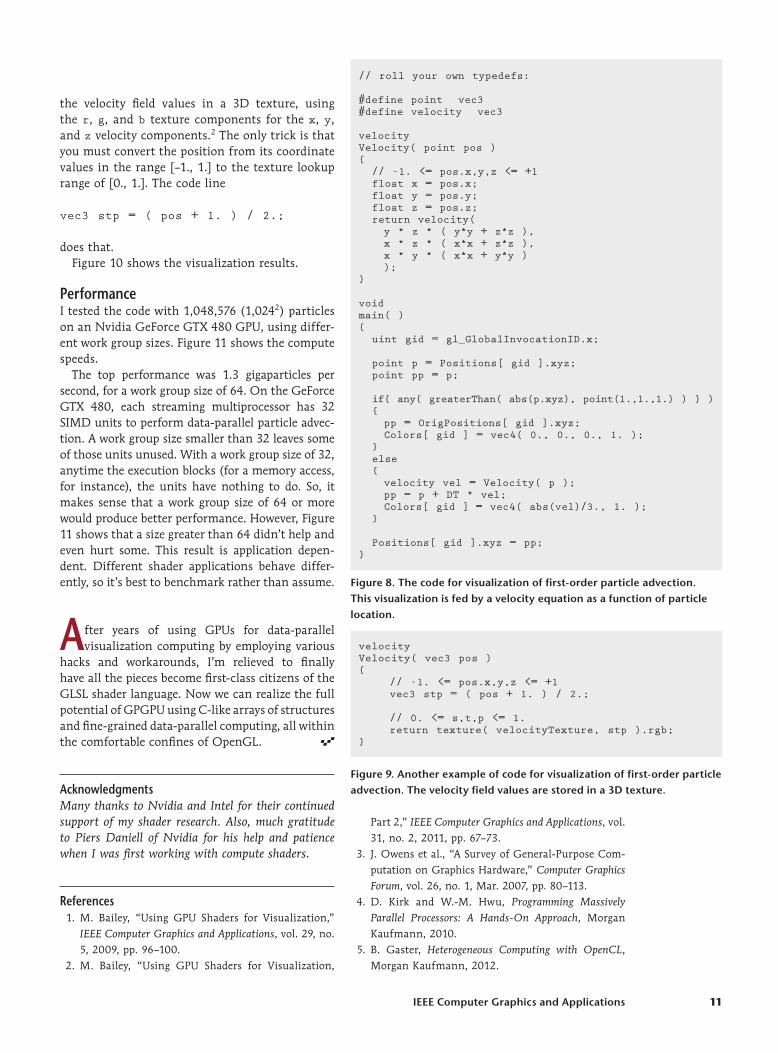
the velocity field values in a 3D texture, using the r, g, and b texture components for the x, y, and z velocity components.2 The only trick is that you must convert the position from its coordinate values in the range [–1., 1.] to the texture lookup range of [0., 1.]. The code line

vec3 stp = ( pos + 1. ) / 2.;

does that.Figure 10 shows the visualization results.

PerformanceI tested the code with 1,048,576 (1,0242) particles on an Nvidia GeForce GTX 480 GPU, using differ-ent work group sizes. Figure 11 shows the compute speeds.

The top performance was 1.3 gigaparticles per second, for a work group size of 64. On the GeForce GTX 480, each streaming multiprocessor has 32 SIMD units to perform data-parallel particle advec-tion. A work group size smaller than 32 leaves some of those units unused. With a work group size of 32, anytime the execution blocks (for a memory access, for instance), the units have nothing to do. So, it makes sense that a work group size of 64 or more would produce better performance. However, Figure 11 shows that a size greater than 64 didn’t help and even hurt some. This result is application depen-dent. Different shader applications behave differ-ently, so it’s best to benchmark rather than assume.

After years of using GPUs for data-parallel visualization computing by employing various

hacks and workarounds, I’m relieved to finally have all the pieces become first-class citizens of the GLSL shader language. Now we can realize the full potential of GPGPU using C-like arrays of structures and fine-grained data-parallel computing, all within the comfortable confines of OpenGL.

AcknowledgmentsMany thanks to Nvidia and Intel for their continued support of my shader research. Also, much gratitude to Piers Daniell of Nvidia for his help and patience when I was first working with compute shaders.

References 1. M. Bailey, “Using GPU Shaders for Visualization,”

IEEE Computer Graphics and Applications, vol. 29, no. 5, 2009, pp. 96–100.

2. M. Bailey, “Using GPU Shaders for Visualization,

Part 2,” IEEE Computer Graphics and Applications, vol. 31, no. 2, 2011, pp. 67–73.

3. J. Owens et al., “A Survey of General-Purpose Com-putation on Graphics Hardware,” Computer Graphics Forum, vol. 26, no. 1, Mar. 2007, pp. 80–113.

4. D. Kirk and W.-M. Hwu, Programming Massively Parallel Processors: A Hands-On Approach, Morgan Kaufmann, 2010.

5. B. Gaster, Heterogeneous Computing with OpenCL, Morgan Kaufmann, 2012.

velocityVelocity( vec3 pos ){ // -1. <= pos.x,y,z <= +1 vec3 stp = ( pos + 1. ) / 2.;

// 0. <= s,t,p <= 1. return texture( velocityTexture, stp ).rgb;}

Figure 9. Another example of code for visualization of first-order particle advection. The velocity field values are stored in a 3D texture.

// roll your own typedefs:

#define point vec3#define velocity vec3

velocityVelocity( point pos ){ // -1. <= pos.x,y,z <= +1 float x = pos.x; float y = pos.y; float z = pos.z; return velocity( y * z * ( y*y + z*z ), x * z * ( x*x + z*z ), x * y * ( x*x + y*y ) );}

voidmain( ){ uint gid = gl_GlobalInvocationID.x;

point p = Positions[ gid ].xyz; point pp = p;

if{ any{ greaterThan( abs(p.xyz), point(1.,1.,1.) ) } ) { pp = OrigPositions[ gid ].xyz; Colors[ gid ] = vec4( 0., 0., 0., 1. ); } else { velocity vel = Velocity( p ); pp = p + DT * vel; Colors[ gid ] = vec4( abs(vel)/3., 1. ); }

Positions[ gid ].xyz = pp;}

Figure 8. The code for visualization of first-order particle advection. This visualization is fed by a velocity equation as a function of particle location.

12 May/June 2013

Visualization Viewpoints

6. A. Munshi et al., OpenCL Programming Guide, Addison-Wesley, 2012.

7. E. Angel and D. Shreiner, Interactive Computer Graphics: A Top-Down Approach with OpenGL, 6th ed., Addison-Wesley, 2011.

8. R. Rost et al., OpenGL Shading Language, Addison-Wesley, 2009.

9. M. Bailey and S. Cunningham, Graphics Shaders: Theory and Practice, 2nd ed., Taylor & Francis, 2012.

Mike Bailey is a professor of computer science at Oregon State University. Contact him at mjb@cs.oregonstate.edu.

Contact department editor Theresa-Marie Rhyne at theresamarierhyne@gmail.com.

Figure 10. A visualization of particle advection. The second image is a magnification of the first image’s upper-right corner. This shows just how incredibly high the particle count can get while still allowing interactive performance.

38 48 64 80 96 112 128 Work group size

Gig

apar

ticl

es/s

ec.

1.4

1.2

1.0

0.8

0.6

Figure 11. Compute shader performance as a function of work group size. These results are application-dependent.