1

Using deep sequencing to characterize the biophysical mechanism of a transcriptional regulatory sequence: SI Appendix Justin B. Kinney, Anand Murugan, Curtis G. Callan Jr., Edward C. Cox

Table of Contents:

1. Supporting experimental procedures a. Plasmid library construction b. Media and growth rates c. Amplicon generation d. Processing of sequence reads e. Library substitution rates f. Post-sort loss of library diversity

2. Supporting theoretical methods a. Overview of mutual information b. Statistical inference using mutual information (justification of Eq. 1) c. Maximizing mutual information leaves some model parameters

undetermined d. Fitting a model to multiple data sets e. Computing mutual information f. Parallel tempering Monte Carlo sampling of model parameters g. Model comparison to literature

3. Supporting information references 4. Supporting information figures

1. Supporting experimental procedures

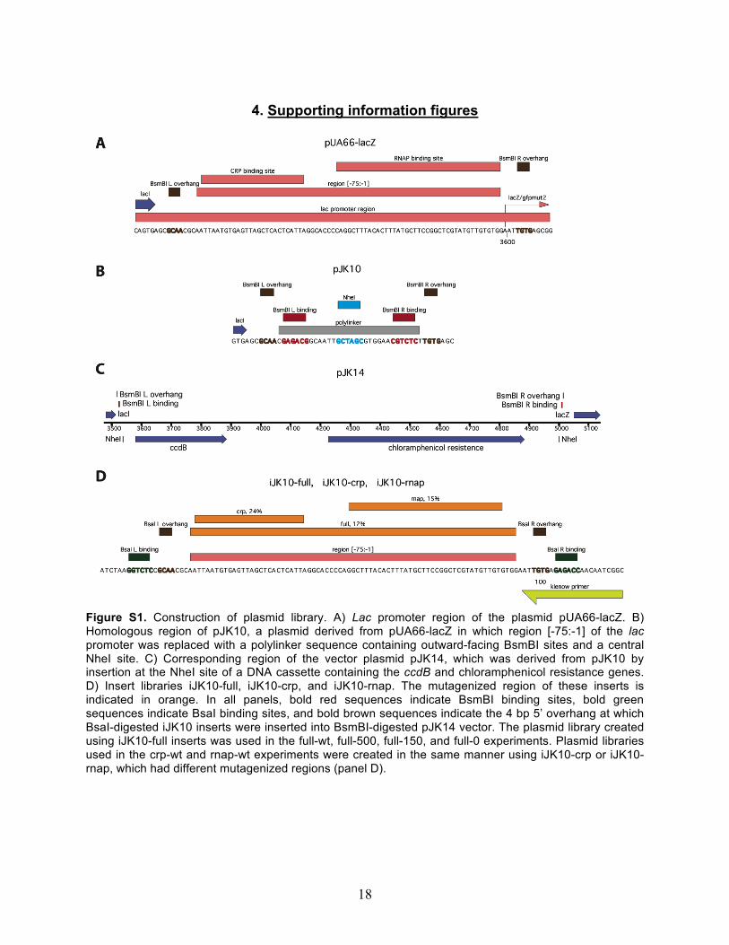
1a. Plasmid library construction Fig. S1 shows the lac promoter region of the plasmid pUA66-lacZ (panel A). Region [-75:-1] of this promoter is bounded on the left by the 4 bp sequence GCAA and on the right by the 4 bp sequence TGTG (brown). To facilitate the replacement of this region with mutant sequences without introducing artificial restriction sites into the lac promoter, we created plasmid pJK10 (Fig. S1B), in which the region between GCAA and TGTG was replaced with a polylinker sequence containing two outward-facing binding sites for the type IIs restriction enzyme BsmBI. Details on how pJK10 was constructed from pUA66-lacZ are provided in Kinney, 2008. BsmBI binds the 6 bp sequence CGTCTC (red) and cuts downstream of this sequence, leaving 5’ overhangs at the bounding sequences GCAA and TGTG. To ease the preparation of plasmid libraries, we further inserted a DNA cassette containing the ccdB gene (see Hartley et al., 2000) into the NheI site of pJK10 (blue), yielding vector pJK14 (Fig. S1C). pJK14 was propagated in DB3.1 E. coli (Invitrogen), a strain immune to the CcdB toxin.

2

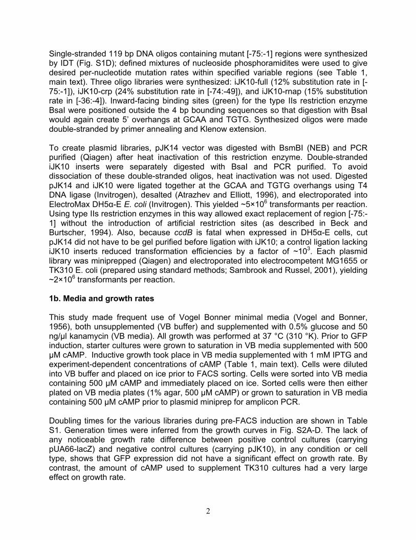
Single-stranded 119 bp DNA oligos containing mutant [-75:-1] regions were synthesized by IDT (Fig. S1D); defined mixtures of nucleoside phosphoramidites were used to give desired per-nucleotide mutation rates within specified variable regions (see Table 1, main text). Three oligo libraries were synthesized: iJK10-full (12% substitution rate in [-75:-1]), iJK10-crp (24% substitution rate in [-74:-49]), and iJK10-rnap (15% substitution rate in [-36:-4]). Inward-facing binding sites (green) for the type IIs restriction enzyme BsaI were positioned outside the 4 bp bounding sequences so that digestion with BsaI would again create 5’ overhangs at GCAA and TGTG. Synthesized oligos were made double-stranded by primer annealing and Klenow extension. To create plasmid libraries, pJK14 vector was digested with BsmBI (NEB) and PCR purified (Qiagen) after heat inactivation of this restriction enzyme. Double-stranded iJK10 inserts were separately digested with BsaI and PCR purified. To avoid dissociation of these double-stranded oligos, heat inactivation was not used. Digested pJK14 and iJK10 were ligated together at the GCAA and TGTG overhangs using T4 DNA ligase (Invitrogen), desalted (Atrazhev and Elliott, 1996), and electroporated into ElectroMax DH5α-E E. coli (Invitrogen). This yielded ~5×106 transformants per reaction. Using type IIs restriction enzymes in this way allowed exact replacement of region [-75:-1] without the introduction of artificial restriction sites (as described in Beck and Burtscher, 1994). Also, because ccdB is fatal when expressed in DH5α-E cells, cut pJK14 did not have to be gel purified before ligation with iJK10; a control ligation lacking iJK10 inserts reduced transformation efficiencies by a factor of ~103. Each plasmid library was miniprepped (Qiagen) and electroporated into electrocompetent MG1655 or TK310 E. coli (prepared using standard methods; Sambrook and Russel, 2001), yielding ~2×106 transformants per reaction. 1b. Media and growth rates This study made frequent use of Vogel Bonner minimal media (Vogel and Bonner, 1956), both unsupplemented (VB buffer) and supplemented with 0.5% glucose and 50 ng/µl kanamycin (VB media). All growth was performed at 37 °C (310 °K). Prior to GFP induction, starter cultures were grown to saturation in VB media supplemented with 500 µM cAMP. Inductive growth took place in VB media supplemented with 1 mM IPTG and experiment-dependent concentrations of cAMP (Table 1, main text). Cells were diluted into VB buffer and placed on ice prior to FACS sorting. Cells were sorted into VB media containing 500 µM cAMP and immediately placed on ice. Sorted cells were then either plated on VB media plates (1% agar, 500 µM cAMP) or grown to saturation in VB media containing 500 µM cAMP prior to plasmid miniprep for amplicon PCR. Doubling times for the various libraries during pre-FACS induction are shown in Table S1. Generation times were inferred from the growth curves in Fig. S2A-D. The lack of any noticeable growth rate difference between positive control cultures (carrying pUA66-lacZ) and negative control cultures (carrying pJK10), in any condition or cell type, shows that GFP expression did not have a significant effect on growth rate. By contrast, the amount of cAMP used to supplement TK310 cultures had a very large effect on growth rate.

3

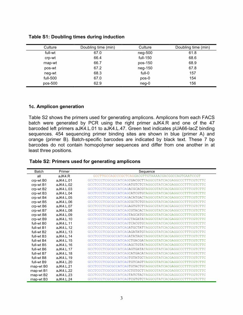
Table S1: Doubling times during induction

Culture Doubling time (min) Culture Doubling time (min) full-wt 67.0 neg-500 61.8 crp-wt 66.4 full-150 68.6

rnap-wt 66.7 pos-150 68.9 pos-wt 67.2 neg-150 67.8 neg-wt 68.3 full-0 157 full-500 67.0 pos-0 154 pos-500 62.9 neg-0 156

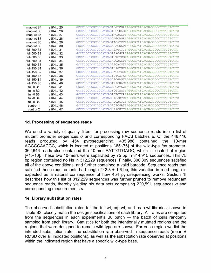
1c. Amplicon generation Table S2 shows the primers used for generating amplicons. Amplicons from each FACS batch were generated by PCR using the right primer aJK4.R and one of the 47 barcoded left primers aJK4.L.01 to aJK4.L.47. Green text indicates pUA66-lacZ binding sequences. 454 sequencing primer binding sites are shown in blue (primer A) and orange (primer B). Batch-specific barcodes are indicated by black text. These 7 bp barcodes do not contain homopolymer sequences and differ from one another in at least three positions. Table S2: Primers used for generating amplicons

Batch Primer Sequence all aJK4.R GCCTTGCCAGCCCGCTCAGGACGTTGTAAAACGACGGCCAGTGAATCCGT

crp-wt B0 aJK4.L.01 GCCTCCCTCGCGCCATCAGCGACGCTTAGGCGTATCACGAGGCCCTTTCGTCTTC crp-wt B1 aJK4.L.02 GCCTCCCTCGCGCCATCAGATGTCTCTAGGCGTATCACGAGGCCCTTTCGTCTTC crp-wt B2 aJK4.L.03 GCCTCCCTCGCGCCATCAGACGCACGTAGGCGTATCACGAGGCCCTTTCGTCTTC crp-wt B3 aJK4.L.04 GCCTCCCTCGCGCCATCAGCATCGTGTAGGCGTATCACGAGGCCCTTTCGTCTTC crp-wt B4 aJK4.L.05 GCCTCCCTCGCGCCATCAGACATGACTAGGCGTATCACGAGGCCCTTTCGTCTTC crp-wt B5 aJK4.L.06 GCCTCCCTCGCGCCATCAGCGCTCTGTAGGCGTATCACGAGGCCCTTTCGTCTTC crp-wt B6 aJK4.L.07 GCCTCCCTCGCGCCATCAGAGTGTCTTAGGCGTATCACGAGGCCCTTTCGTCTTC crp-wt B7 aJK4.L.08 GCCTCCCTCGCGCCATCAGCGTACACTAGGCGTATCACGAGGCCCTTTCGTCTTC crp-wt B8 aJK4.L.09 GCCTCCCTCGCGCCATCAGTAGCATGTAGGCGTATCACGAGGCCCTTTCGTCTTC crp-wt B9 aJK4.L.10 GCCTCCCTCGCGCCATCAGCTAGATATAGGCGTATCACGAGGCCCTTTCGTCTTC full-wt B0 aJK4.L.11 GCCTCCCTCGCGCCATCAGTCACGTGTAGGCGTATCACGAGGCCCTTTCGTCTTC full-wt B1 aJK4.L.12 GCCTCCCTCGCGCCATCAGATGCTATTAGGCGTATCACGAGGCCCTTTCGTCTTC full-wt B2 aJK4.L.13 GCCTCCCTCGCGCCATCAGAGATATGTAGGCGTATCACGAGGCCCTTTCGTCTTC full-wt B3 aJK4.L.14 GCCTCCCTCGCGCCATCAGATATAGCTAGGCGTATCACGAGGCCCTTTCGTCTTC full-wt B4 aJK4.L.15 GCCTCCCTCGCGCCATCAGCTGACGATAGGCGTATCACGAGGCCCTTTCGTCTTC full-wt B5 aJK4.L.16 GCCTCCCTCGCGCCATCAGAGCTGTATAGGCGTATCACGAGGCCCTTTCGTCTTC full-wt B6 aJK4.L.17 GCCTCCCTCGCGCCATCAGAGTGATATAGGCGTATCACGAGGCCCTTTCGTCTTC full-wt B7 aJK4.L.18 GCCTCCCTCGCGCCATCAGCATGACATAGGCGTATCACGAGGCCCTTTCGTCTTC full-wt B8 aJK4.L.19 GCCTCCCTCGCGCCATCAGTGTATGCTAGGCGTATCACGAGGCCCTTTCGTCTTC full-wt B9 aJK4.L.20 GCCTCCCTCGCGCCATCAGTGTCAGTTAGGCGTATCACGAGGCCCTTTCGTCTTC

rnap-wt B0 aJK4.L.21 GCCTCCCTCGCGCCATCAGTGTACTGTAGGCGTATCACGAGGCCCTTTCGTCTTC rnap-wt B1 aJK4.L.22 GCCTCCCTCGCGCCATCAGCTGTGCTTAGGCGTATCACGAGGCCCTTTCGTCTTC rnap-wt B2 aJK4.L.23 GCCTCCCTCGCGCCATCAGTATCTACTAGGCGTATCACGAGGCCCTTTCGTCTTC rnap-wt B3 aJK4.L.24 GCCTCCCTCGCGCCATCAGTCGTGTCTAGGCGTATCACGAGGCCCTTTCGTCTTC

4

rnap-wt B4 aJK4.L.25 GCCTCCCTCGCGCCATCAGACGTCGATAGGCGTATCACGAGGCCCTTTCGTCTTC rnap-wt B5 aJK4.L.26 GCCTCCCTCGCGCCATCAGTGCTGAGTAGGCGTATCACGAGGCCCTTTCGTCTTC rnap-wt B6 aJK4.L.27 GCCTCCCTCGCGCCATCAGTAGACGTTAGGCGTATCACGAGGCCCTTTCGTCTTC rnap-wt B7 aJK4.L.28 GCCTCCCTCGCGCCATCAGCAGCAGATAGGCGTATCACGAGGCCCTTTCGTCTTC rnap-wt B8 aJK4.L.29 GCCTCCCTCGCGCCATCAGTACATCTTAGGCGTATCACGAGGCCCTTTCGTCTTC rnap-wt B9 aJK4.L.30 GCCTCCCTCGCGCCATCAGACAGCATTAGGCGTATCACGAGGCCCTTTCGTCTTC full-500 B1 aJK4.L.31 GCCTCCCTCGCGCCATCAGAGAGCTCTAGGCGTATCACGAGGCCCTTTCGTCTTC full-500 B2 aJK4.L.32 GCCTCCCTCGCGCCATCAGATACGCATAGGCGTATCACGAGGCCCTTTCGTCTTC full-500 B3 aJK4.L.33 GCCTCCCTCGCGCCATCAGTCTGTCGTAGGCGTATCACGAGGCCCTTTCGTCTTC full-500 B4 aJK4.L.34 GCCTCCCTCGCGCCATCAGACGAGCTTAGGCGTATCACGAGGCCCTTTCGTCTTC full-500 B5 aJK4.L.35 GCCTCCCTCGCGCCATCAGATCACGTTAGGCGTATCACGAGGCCCTTTCGTCTTC full-150 B1 aJK4.L.36 GCCTCCCTCGCGCCATCAGTCAGTGTTAGGCGTATCACGAGGCCCTTTCGTCTTC full-150 B2 aJK4.L.37 GCCTCCCTCGCGCCATCAGCACGTGCTAGGCGTATCACGAGGCCCTTTCGTCTTC full-150 B3 aJK4.L.38 GCCTCCCTCGCGCCATCAGTCTCATATAGGCGTATCACGAGGCCCTTTCGTCTTC full-150 B4 aJK4.L.39 GCCTCCCTCGCGCCATCAGCTCGAGTTAGGCGTATCACGAGGCCCTTTCGTCTTC full-150 B5 aJK4.L.40 GCCTCCCTCGCGCCATCAGTGACGACTAGGCGTATCACGAGGCCCTTTCGTCTTC

full-0 B1 aJK4.L.41 GCCTCCCTCGCGCCATCAGAGCATACTAGGCGTATCACGAGGCCCTTTCGTCTTC full-0 B2 aJK4.L.42 GCCTCCCTCGCGCCATCAGTCGTAGTTAGGCGTATCACGAGGCCCTTTCGTCTTC full-0 B3 aJK4.L.43 GCCTCCCTCGCGCCATCAGACTCTCATAGGCGTATCACGAGGCCCTTTCGTCTTC full-0 B4 aJK4.L.44 GCCTCCCTCGCGCCATCAGCTCACTCTAGGCGTATCACGAGGCCCTTTCGTCTTC full-0 B5 aJK4.L.45 GCCTCCCTCGCGCCATCAGACGACTGTAGGCGTATCACGAGGCCCTTTCGTCTTC control 1 aJK4.L.46 GCCTCCCTCGCGCCATCAGACTCGATTAGGCGTATCACGAGGCCCTTTCGTCTTC control 2 aJK4.L.47 GCCTCCCTCGCGCCATCAGCTACGTCTAGGCGTATCACGAGGCCCTTTCGTCTTC

1d. Processing of sequence reads We used a variety of quality filters for processing raw sequence reads into a list of mutant promoter sequences σ and corresponding FACS batches µ. Of the 448,416 reads produced by 454 pyrosequencing, 435,988 contained the 10-mer AGCGCAACGC, which is located at positions [-85:-76] of the wild-type lac promoter. 362,646 reads also contained the 10-mer AATTGTGAGC, which is located at region [+1:+10]. These two 10-mers were separated by 75 bp in 314,915 sequences. This 75 bp region contained no Ns in 312,229 sequences. Finally, 308,309 sequences satisfied all of the above conditions, and further contained a valid barcode. Sequence reads that satisfied these requirements had length 242.3 ± 1.6 bp; this variation in read length is expected as a natural consequence of how 454 pyrosequencing works. Section 1f describes how this list of 312,229 sequences was further pruned to remove redundant sequence reads, thereby yielding six data sets comprising 220,591 sequences σ and corresponding measurements µ. 1e. Library substitution rates The observed substitution rates for the full-wt, crp-wt, and rnap-wt libraries, shown in Table S3, closely match the design specifications of each library. All rates are computed from the sequences in each experiment’s B0 batch — the batch of cells randomly sampled from each library. Statistics for both the intentionally mutated regions and the regions that were designed to remain wild-type are shown. For each region we list the intended substitution rate, the substitution rate observed in sequence reads (mean ± RMSD over all indicated positions), as well as the substitution rate observed at positions within the indicated region that have a specific wild-type base.

5

Table S3: Observed substitution rates

Target Observed Observed sub. % by wild-type base Batch Region sub. % sub. % A C G T

full-wt B0 [-75:-1] 12 11.6 ± 1.9 12.0 ± 0.5 13.8 ± 0.8 12.6 ± 0.5 9.2 ± 0.4 crp-wt B0 [-74:-49] 24 23.3 ± 3.4 25.2 ± 1.0 27.3 ± 0.4 24.9 ± 0.5 19.4 ± 1.0 crp-wt B0 [-75],[-48:-1] 0 0.28 ± 0.17 0.28 ± 0.13 0.47 ± 0.16 0.23 ± 0.12 0.16 ± 0.08

rnap-wt B0 [-39:-4] 15 15.2 ± 2.0 16.1 ± 0.7 16.2 ± 0.6 17.4 ± 1.1 13.1 ± 0.5 rnap-wt B0 [-75:-40],[-3:-1] 0 0.17 ± 0.08 0.20 ± 0.06 0.22 ± 0.05 0.13 ± 0.05 0.11 ± 0.10

The variation among positions that share a given wild-type base is roughly consistent with the expected statistical fluctuations (~0.5%) due to each B0 batch containing only ~5,000 sequences. However, the substitution rates for positions corresponding to different wild-type bases show significant systematic differences. This position-to-position variation is probably due primarily to variations in the nucleoside phosphoramidite mixtures used for synthesizing each position. Importantly, however, positions at which no variation was specified in the design of the sequence libraries still showed a nonzero substitution rate, ranging between 0.1% and 0.5%. By contrast, the observed substitution rate within the control amplicon libraries, which were prepared directly from pUA66-lacZ plasmid (containing the wild-type lac promoter), was 0.017 ± 0.026 %. This difference suggests that the substitutions observed in the supposedly wild-type regions of crp-wt and rnap-wt did not result from sequencing errors or errors in amplicon PCR, but rather from substitutions that occurred either during DNA synthesis or during the construction of reporter construct libraries. Supporting evidence for this hypothesis — that these undesired substitutions occurred prior to FACS — is given by Fig. S3B, which shows that observed substitutions at positions -37 and -14 in the crp-wt experiment are significantly informative about flow cytometry measurements. 1f. Post-sort loss of library diversity The validity of our analysis requires that all entries in our data sets arise from different FACS-sorted cells and thereby represent independent measurements of promoter activity. It was therefore important that we not only FACS-sort a sufficient number of cells, but that enough of these cells actually produce sequenced amplicons. In our six experiments we sorted 100,000 flow-cytometer-detected "events" into each FACS batch. Plating 0.1% of the cells in each batch immediately afterward, we observed ~70 equal-sized colonies per plate. We concluded that each batch received ~70,000 viable cells — i.e. that ~70% of detected "events" represented viable cells. It appears, however, that a large loss in library diversity occurred between the sorting of these cells and the sequencing of amplicons, and that as a result our experiment yielded amplicons from only ~13,000 independently sorted cells per batch. We determined this library reduction as follows.

6

After FACS, we miniprepped the plasmids within each batch, used these plasmids as template for amplicon PCR, then sequenced the resulting amplicons. If a particular batch originally contained N independently sorted (viable) cells, each cell containing a different CRM sequence, and n sequences in our final data set derived from this batch, the probability pk of a given sequence occurring k times in this batch should follow what one would expect from sampling n out of N objects with replacement. Using a Poisson approximation to this binomial probability (a valid approximation because N, n >> 1),

(S1) .

Now consider the probability fk of a sequence randomly drawn from this batch having exactly k occurrences therein:

(S2) .

In particular, consider

(S3) .

These quantities, f1 and f2, are readily determined from our data sets. Since we also know n, we can use f1 and f2 to estimate the effective population size Neff of sorted cells that gave rise to sequenced amplicons. In fact, this can be done in multiple ways:

(S4) Neff ,1 = −n

log(f1)   and   Neff ,2 = n f1

f2.

For the full-wt, crp-wt, and rnap-wt experiments, Table S4 shows the total number (n) of sequences found in batch B0, the number of distinct sequences in this batch, the quantities f1 and f2, the two resulting estimates Neff,1 and Neff, and the total number of distinct sequences observed across all batches B0-B9.

Table S4: Post-sort library reduction

Data set Total in B0 Distinct in B0 f1 f2 Neff,1 Neff,2 Distinct in B0-B9 full-wt 7,680 5,799 0.57 0.26 13,946 16,801 50,518 crp-wt 5,805 4,347 0.56 0.26 10,256 12,328 45,050

rnap-wt 6,453 4,748 0.55 0.25 10,926 13,998 43,818

In all three cases, both Neff,1 and Neff,2 are ~12,000. By contrast, each experiment generated ~45,000 distinct sequences across all 10 batches — nearly 10 times the

7

number of distinct sequences within each individual batch. We therefore concluded that, prior to sorting, the library size in each experiment was >> 45,000, whereas after sorting the number of distinct sequences within each batch dropped from ~70,000 to ~12,000. Similar Neff values were found for each of the 45 batches in our six experiments, suggesting uniform library diversity loss across all FACS batches. Because of this reduction in library diversity, a single sequence appearing multiple times in the same batch was most likely to result from a single sorted cell giving rise to multiple sequenced amplicons, not from different sorted cells each giving rise to one sequenced amplicon. In other words, the appearance of one sequence multiple times in a single batch would represent a single measurement, not multiple independent measurements. To ensure that our analysis used only independent measurements, we performed computations using data sets in which each distinct sequence in each batch was listed only once. This left a total of 220,591 non-redundant sequences across our six experiments; the number of such sequences remaining in each experiment's data set is shown in Table 1 of the main text.

2. Supporting theoretical methods 2a. Overview of mutual information Mutual information provides a fundamental measure of dependence between any two random variables, say x and y. The mutual information I(x;y) between two such variables is computed from their joint distribution p(x,y) as

(S5) .

If either variable is continuous, the corresponding summation is replaced by an integral. I(x;y) can thus be computed regardless of whether both variables are discrete (such as a base b and batch µ), one variable is discrete and the other is continuous (such as predicted binding energy ε and batch µ), or both variables are continuous. I(x;y) is clearly symmetric, i.e. I(x;y) = I(y;x). Also, a basic result of information theory is that I(x;y) ≥ 0, with zero information only if x and y are independent, i.e. p(x,y) = p(x)p(y). Another basic property of mutual information is that I(x;y) doesn't change if either x or y undergoes an invertible transformation. To see this, consider some invertible transformation z(x) of x. Then I(z;y) = I(x;y) (regardless of whether y is continuous or discrete) because

8

(S6) .

This has important implications for what kinds of parameters we can infer when fitting models to our data (see Sec. 2c). Mutual information provides a measure of dependence, much as correlation does. In fact, if x and y are two correlated Gaussian random variables, there exists a simple relationship between I(x;y) and the correlation coefficient ρ between x and y. To see this, assume that both x and y have mean 0 and variance 1. Then

(S7)

p(x,y) = 1

2π Λexp −

12

x y⎡⎣

⎤⎦ Λ

−1 xy

⎡

⎣⎢⎢

⎤

⎦⎥⎥

⎛

⎝⎜

⎞

⎠⎟ where Λ =

1 ρρ 1

⎡

⎣⎢⎢

⎤

⎦⎥⎥.

Plugging this into Eq. S5 gives

(S8) .

Note that I(x;y) = 0 for , and as . Because I(x;y) is invariant under any affine transformation of x or y (via Eq. S6), Eq. S8 holds for all correlated Gaussian variables x and y with correlation coefficient ρ. Despite the simplicity of Eq. S5, actually estimating mutual information from finite data is nontrivial. The steps we took to do this are described in Sec. 2e. 2b. Statistical inference using mutual information (justification of Eq. 1) Our rationale for sampling model parameters according to Eq. 1 comes from a relationship between mutual information and a quantity called "error-model-averaged likelihood", first described in Kinney et al., 2007. Kinney et al. considered the problem of fitting a sequence-dependent model of some biological activity x to noisy measurements µ of this activity for a large number N of sequences σ. They considered a particular case where the sequences σ were the intergenic regions of S. cerevisiae and the measurements µ were the fluorescence intensities observed in ChIP-chip (Lee et al., 2002) or protein binding microarray (Mukherjee et al., 2004) experiments on yeast

9

transcription factors. The models they considered consisted of energy matrices together with energy thresholds. Model predictions were binary — "bound" or "not bound" —corresponding to whether an intergenic sequence contained at least one site with energy below the specified threshold. Despite the specific nature of their interests, though, the inference issues Kinney et al. addressed were quite general. To determine model parameters θ, one can sample θ according to the likelihood of actually seeing the set of observations {µi} given the model predictions {xi}, where the index i=1,...,N runs over all the sequences assayed, and xi is the prediction assigned to sequence σi. Normally, one would compute this likelihood using prior knowledge of an “error model” p(µ|x), which specifies the distribution of measurements µ to be expected given a particular value for the underlying quantity-of-interest x. Likelihood is expressed in terms of this error model according to the standard formula,

(S9) p({µi } | {σ i },θ) = p({µi } | {xi }) = p(µi

i=1

N

∏ | xi ) .

For Kinney et al., p(µ|x) represented the distribution of microarray intensities expected from sequences that either contained (x = "bound") or did not contain (x = "not bound") a protein binding site. Since Kinney et al. had no a priori knowledge of the experimental error model p(µ|x), they instead proposed the use of “error-model-averaged” likelihood, computed by averaging the standard likelihood (Eq. S9) over all possible error models p(µ|x) according to an explicit prior on the space of possible error models. They showed that, under very general assumptions, error-model-averaged likelihood has a remarkably simple structure:

(S10) pema({µi } | {σ i },θ) = p(µi | xi )

i=1

N

∏all possible p(µ|x)

= 2N[I(x;µ)−H(µ)−Δ ] .

where I(x;µ) is the mutual information between measurements µ and model predictions x, H(µ) is the entropy of the experimental measurements (which does not depend on model parameters θ) and Δ is a positive number that depends on the particular prior used to compute the average over possible error models p(µ|x). Kinney et al. further showed that, under mild assumptions on the prior, as , meaning that Δ can be ignored in the large N limit. Finally, Kinney et al. showed that EMA likelihood could be computed exactly if one assumed a Dirichlet prior on the space of error models. However, the resulting formula for EMA likelihood caused problems in the analysis presented in the present paper; it gave likelihood landscapes that were unreasonably rugged and thus prevented us from

10

optimizing model parameters. This ruggedness probably stems from the fact that the Dirichlet prior used by Kinney et al. does not require that p(µ|x) be similar for similar values of x (and fixed µ). By contrast, any biophysically reasonable prior on the space of error models should require such smoothness in the x-direction. We therefore took a different approach that, while not proven mathematically, works very well in practice: we assumed that error-model-averaged likelihood could be safely approximated as

(S11) pema({µi } | {σ i },θ) = const × 2NIsmooth (x;µ) . where Ismooth(x;µ) is computed using a Gaussian-smoothed version of the joint distribution p(µ,x) in the formula for mutual information (Eq. S5). Eq. S11 is just a more explicit form of Eq. 1 in the main text. Sec. 2e describes how this smoothing of p(µ,x) was done. 2c. Maximizing mutual information leaves some model parameters undetermined Our inability to determine certain model parameters — the multiplicative scale of εc and εr when fitting individual energy matrices, and τmax and Cr when fitting τ — arises from a basic property of mutual information: transforming model predictions x in a way that does not change their rank order leaves the predictive information I(x;µ) unchanged (see Eq. S6). Thus multiplying εc or εr by a constant leaves I(εc;µ) and I(εr;µ) invariant. Similarly, changing τmax has no effect on I(τ;µ). It is also true that changing Cr has no effect I(τ;µ), though this is not as obvious. Eq. 2 of the main text can be rewritten

(S12)

Here, τ is an invertible function of η for all Cr > 0, and so I(τ;µ) = I(η;µ) by Eq. S6. But the expression for η makes no reference to Cr. The value of Cr therefore has no influence on I(τ;µ), and cannot be inferred by fitting τ to data. It may seem odd that inferring models for εc and εr by fitting τ allowed us to determine these energies in kcal/mol, whereas separately fitting models for these binding energies did not. In general, which parameters one can or cannot determine depends on the specific analytic form of the model being considered. We have found that simpler (more linear) models tend to have more unconstrained parameters. We cannot yet make definitive statements on this matter, though, and which parameters one can or cannot fit in any given model must be assessed on a case-by-case basis. Kinney, 2008, shows how to perform this assessment analytically.

11

2d. Fitting a model to multiple data sets A single biophysical model can be fit to multiple data sets using a straightforward generalization of Eq. 1. One reason for doing so is that, by using all the data in hand, one can minimize error bars on inferred model parameters. More compelling, though, is the fact that letting select parameters vary between data sets can shed light on the molecular mechanisms responsible for modulating transcriptional activity in response to different inducing conditions or genomic backgrounds. Generalizing the relationship between mutual information and likelihood to data from multiple experiments is straightforward:

(S13) p(multiple data sets|model) = p(data set j|model) = const × 2

Nj I(xj ;µ j )j∑

j∏

where j indexes different data sets, xj denotes model predictions specific to experiment j, µj denotes corresponding measurements, and Nj is the number of independent measurements in that data set. This relation is valid regardless of which parameters are experiment-specific and which are shared across all experiments. Model parameters can be sampled according to this distribution the same way they are sampled according to Eq. 1. 2e. Computing mutual information Despite the fundamental role that mutual information plays in information theory, there are a variety of ways to estimate mutual information from finite amounts of data. Which technique one should use depends on the specific context of the calculation. In this paper, there are three contexts in which we compute mutual information, each requiring its own method:

i. Computing I(b;µ) for information footprints ii. Comparing I(τ;µ) to I(εr,εc;µ) iii. Computing I(x;µ) for sampling model parameters

Computing I(b;µ) for information footprints We used the following procedure (schematized in Fig. S6A) to compute the I(b;µ) values in information footprints. For a given nucleotide position within the aligned N sequences σ, we determined the fraction of the time that base b occurred at that position in a sequence recovered from batch µ. From this occurrence frequency, f(b,µ), one can compute the “naive” mutual information between bases b and batches µ:

(S14)

12

where f(b) and f(µ) are the marginal distributions of f(b,µ). However, finite sample effects will typically cause Eq. S14 to overestimate the true mutual information — i.e. the value of I(b;µ) one would find if one was able to collect an infinite amount data. If f(b,µ) is well-sampled at all values of b and µ, though, one can analytically compute the correction to this information value (Treves and Panzeri, 1995),

(S15) ,

where nb = 4 is the number of possible bases b and nµ is the number of batches µ (5 or 10 in our experiments). Using the first two terms on the right-hand-side of Eq. S15 thus allows one to compute an estimate of I(b;µ) that is essentially unbiased. This is the formula we used to estimate all I(b;µ) values shown in Fig. 2 and Fig. S3. To determine error bars on each of these I(b;µ) information values, we computed a large number of naive information estimates evaluated on random subsamples of the data consisting of half the sequences σ. The variance in these values across different subsamples was used to compute the uncertainty in I(b;µ):

(S16) .

Comparing I(τ;µ) to I(εr,εc;µ) As in our computation of I(b;µ), we looked for absolute information values with error bars when comparing I(τ;µ) to I(εr,εc;µ). There were two new issues we had to deal with, however. The first is that model predictions x are continuous values, not categorical variables (like bases b), and some regularization method was required to estimate a well-sampled joint distribution p(x,µ). To compute I(τ;µ), we took advantage of the fact that transformations of τ that do not change the rank order of these predictions do not affect I(τ;µ). Specifically, we equipartitioned τ values among 100 bins, thus reassigning each prediction x to a bin number X=1,2,...,100 according to its rank order. To compute I(εc,εr;µ), we equipartitioned both εc and εr into 15 bins each, then used X to number each of the resulting 225 bins. The observed frequency distribution f(X,µ) between these bin numbers and batches µ was then used to compute Inaive(X;µ) in both cases.   The second issue is that, unlike in estimating I(b;µ), the frequency table f(X,µ) typically did not contain many counts for every pair of X and µ. The analytic correction in Eq. S15, used for countering the upward bias in the naive estimate of mutual information, was therefore invalid. Instead we used the “direct” method of information estimation described by Slonim et al., 2005 (following the initial proposal by Strong et al., 1998). We computed f(X;µ) and the corresponding value for for 25 subsamples of

13

the data for each of the three subsample percentages: 83%, 63%, and 50%. The interpolation scheme described in Slonim et al. was then used to read off I(X;µ) in the infinite data limit from the mean values of , , and . Error bars on I(X;µ) were computed in the same way as for information footprints:

(S17) .

Computing I(x;µ) for sampling model parameters The method of Slonim et al., 2005, is too computationally demanding to use as part of the Monte Carlo procedure we used to infer model parameters. We therefore used an alternate procedure (Fig. S6B) to determine I(x;µ) for use in Eq. 1. After assigning a rank order R to each model prediction we convolved the observed frequency distribution f(R,µ) in the R dimension with a Gaussian having a standard deviation equal to 4% the number of data points. This generated a regularized distribution p(R,µ) , which we used in Eq. S5 to compute I(R;µ) = I(x;µ). 2f. Parallel tempering Monte Carlo sampling of model parameters We used a custom parallel tempering Monte Carlo algorithm (Earl and Deem, 2005) to sample parameters according to their likelihood in Eq. S11. We note that it is valid to assume p(θ|{µi},{σi}) = const × p({µi}|{σi},θ) if there is no need for a strong prior distribution p(θ) on model parameters θ. The algorithm that follows can be readily altered to accommodate such a prior, however, if one is needed. The parallel tempering Monte Carlo algorithm we used to sample parameters θ worked as follows.

1. We initiated K processes (using K = 40 or 100). For each process k = 0,1,...,K-1 we

a. Chose an initial value for model parameters θk b. Computed the mutual information I(xk;µ) resulting from this choice of

parameters θk c. Assigned an “inverse temperature” βk ≤ 1 to each process k, with β0 = 1 for

process k = 0. We chose log10 βk values to be evenly spaced between 1 and either 3 or 4

2. We then iterated the following steps simultaneously for all processes k.

a. Randomly perturbed model parameters b. Computed the predictive information resulting from perturbed

parameters c. Replaced with with probability

14

d. Recorded

3. During this iteration, we would periodically choose two processes, k,m < K and switch parameter values with probability min(1,2−N[βk −βm ][I(xk ;µ)−I(xm ;µ)] ) . This is the defining step in parallel tempering Monte Carlo algorithm (Earl and Deem, 2005).

4. We used the resulting ensemble of parameter values θ0 from process k = 0 to

determine the best value, the mean value, and the RMSD uncertainty in each parameter in θ. Parameter ensembles from all other processes k = 1,2,...,K-1 were used only for diagnostic purposes, not for estimating model parameters.

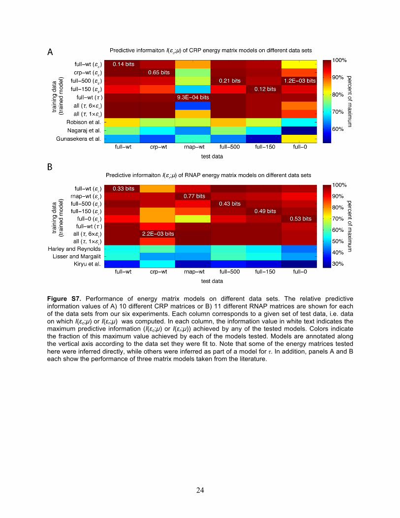
In other words, this algorithm uses multiple particles (K of them) to explore the probability landscape (over the space of model parameters θ) defined by Eq. 1. Different particles have different “temperatures”; hotter particles (lower βk) experience a smoother landscape and are less prone to get stuck in local optima, while cooler particles (higher βk) are more sensitive to the shape of the landscape and can locate optima more precisely that hotter particles. Most of the time, particles explore the probability landscape according to the normal Metropolis algorithm (step 2). The power of parallel tempering comes from the periodic execution of step 3. This allows hotter particles and cooler particles to trade parameter values if the hotter particle is found to be in a higher probability state, since such a situation would suggest that the cooler particle was stuck in a local optimum and that the hotter particle had found a better solution. Parallel tempering Monte Carlo thereby provides rigorous sampling of parameters θ while enabling the quick identification of global optima even in the presence of many local optima; normal Monte Carlo, on the other hand, is very prone to getting stuck in local optima. 2g. Model comparison to literature Performance of CRP and RNAP energy matrices on our six data sets Fig. S7 compares the performance of our inferred CRP and RNAP energy matrices to three CRP matrices and three RNAP matrices found in the literature. Every one of our inferred matrices performs better on every one of our data sets (with two exceptions) than any of the matrices taken from the literature. One exception is that the CRP energy matrix fit to full-wt data performs equally well on full-0 data as the model of Gunasekera et al.,1992. The other exception is the performance of CRP matrices on the rnap-wt data set. The information values in this column are somewhat suspect, though, because the CRP binding site was not intentionally mutagenized in the rnap-wt experiment; listed information values (all less than 0.001 bits) are significantly nonzero only because a small fraction of sequences from the rnap-wt experiment have spurious mutations in their CRP binding sites (see Table S3). The dearth of sequences with mutated CRP

15

binding sites may have caused problems for our estimation of I(εc;µ). This same concern applies to the performance of RNAP matrices on crp-wt data. CRP and RNAP matrices gleaned from the literature The energy matrices derived from Harley and Reynolds, 1987, Lisser and Margalit, 1993, and Robison et al., 1998 were constructed from either aligned CRP binding sites or from aligned σ70 promoters (having an 18 bp spacing between their -10 and -35 elements) using the method of Berg and von Hippel (Berg and von Hippel, 1987; Stormo, 2000): for each list of aligned sequences, energy matrix elements Ebi were computed (in arbitrary units) as

(S18)

where ci(b) is the number of sites that have base b at position i, N is the total number of sites, and p(b) is the frequency of base b in the intergenic DNA of E. coli (which has a GC content of 43.4%). The RNAP energy matrix reported in Kiryu et al. (2005) was derived from microarray expression data using an algorithm written by the authors; matrix elements were gleaned from the bottom panel of Fig. 4 in that publication. The CRP energy matrix reported in Nagaraj et al. (2008) was found using the QPMEME algorithm (Djordjevic et al., 2003) applied to CRP SELEX data. The CRP energy matrix quoted for Gunasekera et al. (1992) was constructed from the measured ΔΔG values listed in Table 1 of that publication; ΔΔG = 5.2 kcal/mol was assumed for values listed as ΔΔG > 5.2 kcal/mol. Thermodynamic parameters from Kuhlman et al., 2007 The value of fcAMP = 240 ± 13, listed for TK310 cells in Table 2 of Kuhlman et al., 2007, corresponds to exp[-εi / RT] with a CRP-RNAP interaction energy of εi = -3.37 ± 0.03 kcal/mol. Kuhlman et al. also predicts that the concentration of active intracellular CRP in TK310 cells is related to the concentration of cAMP used to supplement growth media via Cc = [cAMP]/(320 µM). This implies that Cc

full-500 = 100.19 and Ccfull-150 = 10-0.33,

both of which are about 20-times larger than our inferred values (Fig. 4B, main text).

3. Supporting information references

Atrazhev A, Elliott J (1996) Simplified desalting of ligation reactions immediately prior to electroporation into E. coli. Biotechniques 21:1024.

16

Beck R, Burtscher H (1994) Introduction of arbitrary sequences into genes by use of class IIs restriction enzymes. Nucl Acids Res 22:886-887. Berg OG, von Hippel PH (1987) Selection of DNA binding sites by regulatory proteins. Statistical-mechanical theory and application to operators and promoters. J Mol Biol 193:723-750. Djordjevic M, Sengupta AM, Shraiman BI (2003) A biophysical approach to transcription factor binding site discovery. Genome Res 13:2381-2390. Earl DJ, Deem MW (2005) Parallel tempering: Theory, applications, and new perspectives. Phys Chem Chem Phys 7:3910. Hartley JL, Temple GF, Brasch MA (2000) DNA cloning using in vitro site-specific recombination. Genome Res 10:1788-1795. Kinney JB (2008) Biophysical models of transcriptional regulation from sequence data. Ph.D. Dissertation, Princeton University. Kiryu H, Oshima T, Asai K (2005) Extracting relations between promoter sequences and their strengths from microarray data. Bioinformatics 21:1062-1068. Lee TI, et al. (2002). Transcriptional regulatory networks in Saccharomyces cerevisiae. Science 298, 799-804. Lisser S, Margalit H (1993) Compilation of E. coli mRNA promoter sequences. Nucl Acids Res 21:1507-1516. Mukherjee S, et al. (2004) Rapid analysis of the DNA-binding specificities of transcription factors with DNA microarrays. Nat Genet 36:1331-1339. Nagaraj VH, O'Flanagan RA, Sengupta AM (2008) Better estimation of protein-DNA interaction parameters improve prediction of functional sites. BMC Biotechnol 8:94. Robison K, McGuire AM, Church GM (1998) A comprehensive library of DNA-binding site matrices for 55 proteins applied to the complete Escherichia coli K-12 genome. J Mol Biol 284:241-254. Sambrook J, Russell DW (2001) Molecular Cloning (Cold Spring Harbor, NY: Cold Spring Harbor Laboratory). Slonim N, Atwal GS, Tkacik G, Bialek W (2005) Estimating mutual information and multi-information in large networks. http://arxiv.org/abs/cs/0502017. Strong SP, Koberle R, de Ruyter van Steveninck R, Bialek W (1998) Entropy and Information in Neural Spike Trains. Phys Rev Lett 80:197-200.

17

Stormo GD (2000) DNA binding sites: representation and discovery. Bioinformatics 16:16-23. Treves A, Panzeri S (1995) The upward bias in measures of information derived from limited data samples. Neural Comput 7:399-407. Vogel H, Bonner D (1956) Acetylornithinase of Escherichia coli: partial purification and some properties. J Biol Chem 218:97-106.

18

4. Supporting information figures

Figure S1. Construction of plasmid library. A) Lac promoter region of the plasmid pUA66-lacZ. B) Homologous region of pJK10, a plasmid derived from pUA66-lacZ in which region [-75:-1] of the lac promoter was replaced with a polylinker sequence containing outward-facing BsmBI sites and a central NheI site. C) Corresponding region of the vector plasmid pJK14, which was derived from pJK10 by insertion at the NheI site of a DNA cassette containing the ccdB and chloramphenicol resistance genes. D) Insert libraries iJK10-full, iJK10-crp, and iJK10-rnap. The mutagenized region of these inserts is indicated in orange. In all panels, bold red sequences indicate BsmBI binding sites, bold green sequences indicate BsaI binding sites, and bold brown sequences indicate the 4 bp 5’ overhang at which BsaI-digested iJK10 inserts were inserted into BsmBI-digested pJK14 vector. The plasmid library created using iJK10-full inserts was used in the full-wt, full-500, full-150, and full-0 experiments. Plasmid libraries used in the crp-wt and rnap-wt experiments were created in the same manner using iJK10-crp or iJK10-rnap, which had different mutagenized regions (panel D).

19

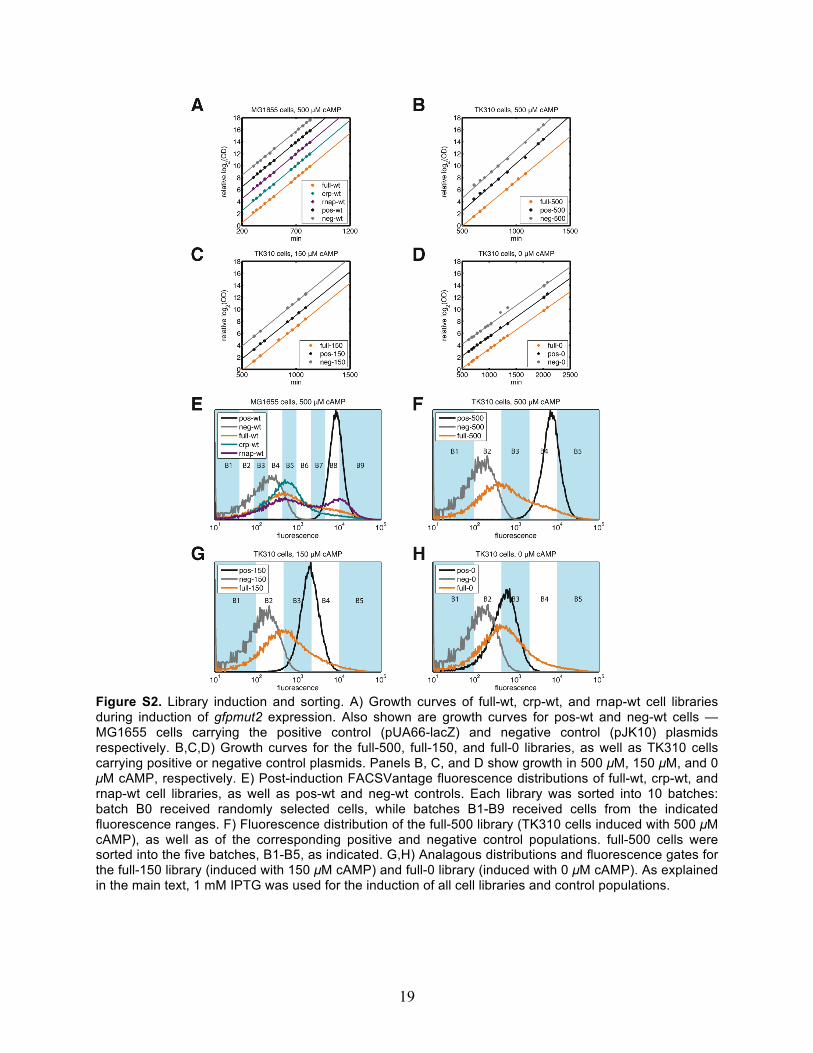
Figure S2. Library induction and sorting. A) Growth curves of full-wt, crp-wt, and rnap-wt cell libraries during induction of gfpmut2 expression. Also shown are growth curves for pos-wt and neg-wt cells — MG1655 cells carrying the positive control (pUA66-lacZ) and negative control (pJK10) plasmids respectively. B,C,D) Growth curves for the full-500, full-150, and full-0 libraries, as well as TK310 cells carrying positive or negative control plasmids. Panels B, C, and D show growth in 500 µM, 150 µM, and 0 µM cAMP, respectively. E) Post-induction FACSVantage fluorescence distributions of full-wt, crp-wt, and rnap-wt cell libraries, as well as pos-wt and neg-wt controls. Each library was sorted into 10 batches: batch B0 received randomly selected cells, while batches B1-B9 received cells from the indicated fluorescence ranges. F) Fluorescence distribution of the full-500 library (TK310 cells induced with 500 µM cAMP), as well as of the corresponding positive and negative control populations. full-500 cells were sorted into the five batches, B1-B5, as indicated. G,H) Analagous distributions and fluorescence gates for the full-150 library (induced with 150 µM cAMP) and full-0 library (induced with 0 µM cAMP). As explained in the main text, 1 mM IPTG was used for the induction of all cell libraries and control populations.

20

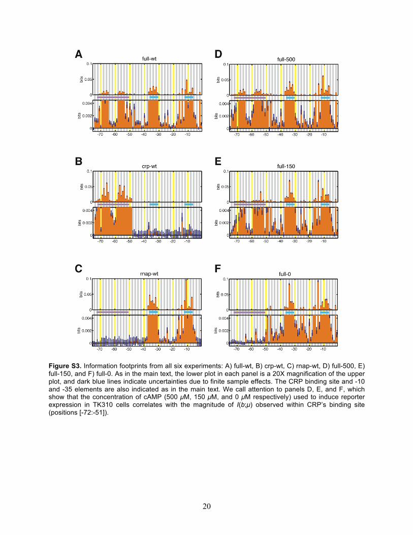
Figure S3. Information footprints from all six experiments: A) full-wt, B) crp-wt, C) rnap-wt, D) full-500, E) full-150, and F) full-0. As in the main text, the lower plot in each panel is a 20X magnification of the upper plot, and dark blue lines indicate uncertainties due to finite sample effects. The CRP binding site and -10 and -35 elements are also indicated as in the main text. We call attention to panels D, E, and F, which show that the concentration of cAMP (500 µM, 150 µM, and 0 µM respectively) used to induce reporter expression in TK310 cells correlates with the magnitude of I(b;µ) observed within CRP’s binding site (positions [-72:-51]).

21

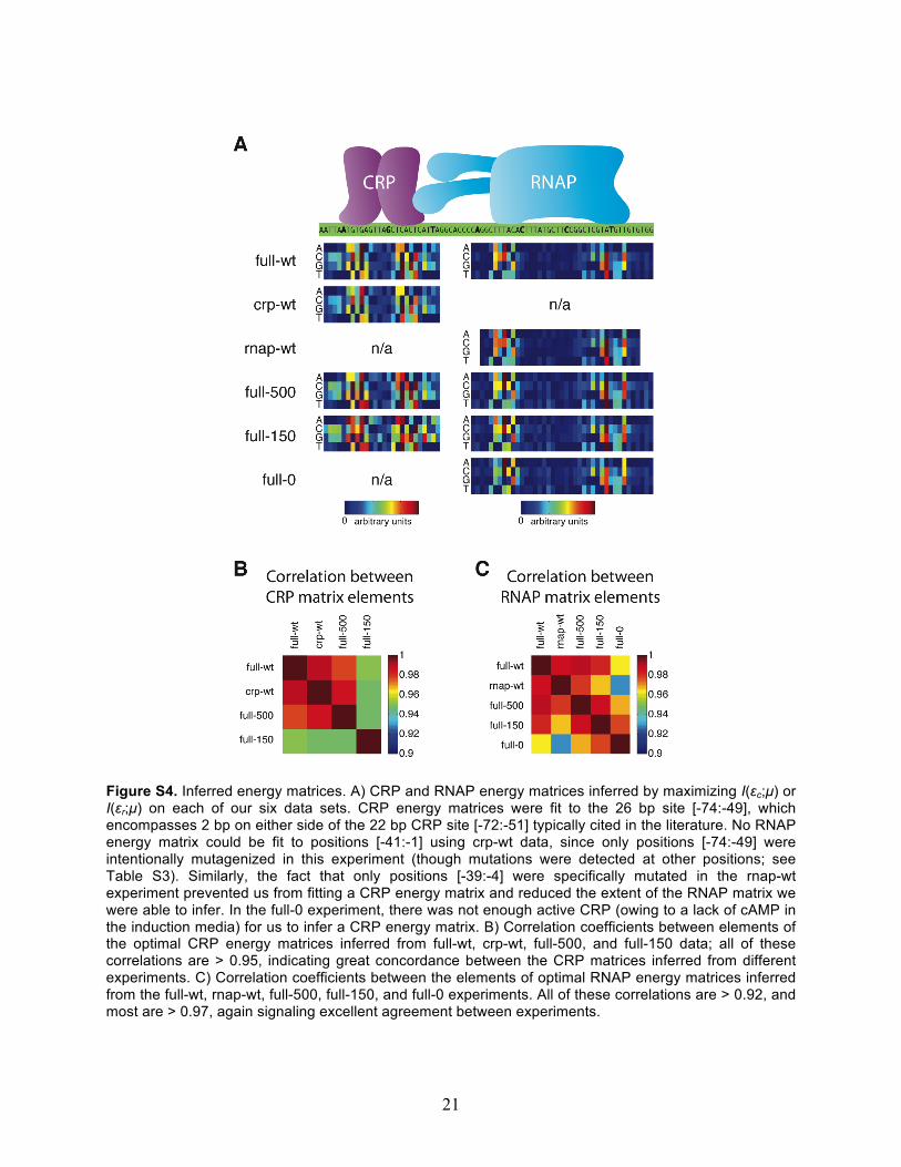
Figure S4. Inferred energy matrices. A) CRP and RNAP energy matrices inferred by maximizing I(εc;µ) or I(εr;µ) on each of our six data sets. CRP energy matrices were fit to the 26 bp site [-74:-49], which encompasses 2 bp on either side of the 22 bp CRP site [-72:-51] typically cited in the literature. No RNAP energy matrix could be fit to positions [-41:-1] using crp-wt data, since only positions [-74:-49] were intentionally mutagenized in this experiment (though mutations were detected at other positions; see Table S3). Similarly, the fact that only positions [-39:-4] were specifically mutated in the rnap-wt experiment prevented us from fitting a CRP energy matrix and reduced the extent of the RNAP matrix we were able to infer. In the full-0 experiment, there was not enough active CRP (owing to a lack of cAMP in the induction media) for us to infer a CRP energy matrix. B) Correlation coefficients between elements of the optimal CRP energy matrices inferred from full-wt, crp-wt, full-500, and full-150 data; all of these correlations are > 0.95, indicating great concordance between the CRP matrices inferred from different experiments. C) Correlation coefficients between the elements of optimal RNAP energy matrices inferred from the full-wt, rnap-wt, full-500, full-150, and full-0 experiments. All of these correlations are > 0.92, and most are > 0.97, again signaling excellent agreement between experiments.

22

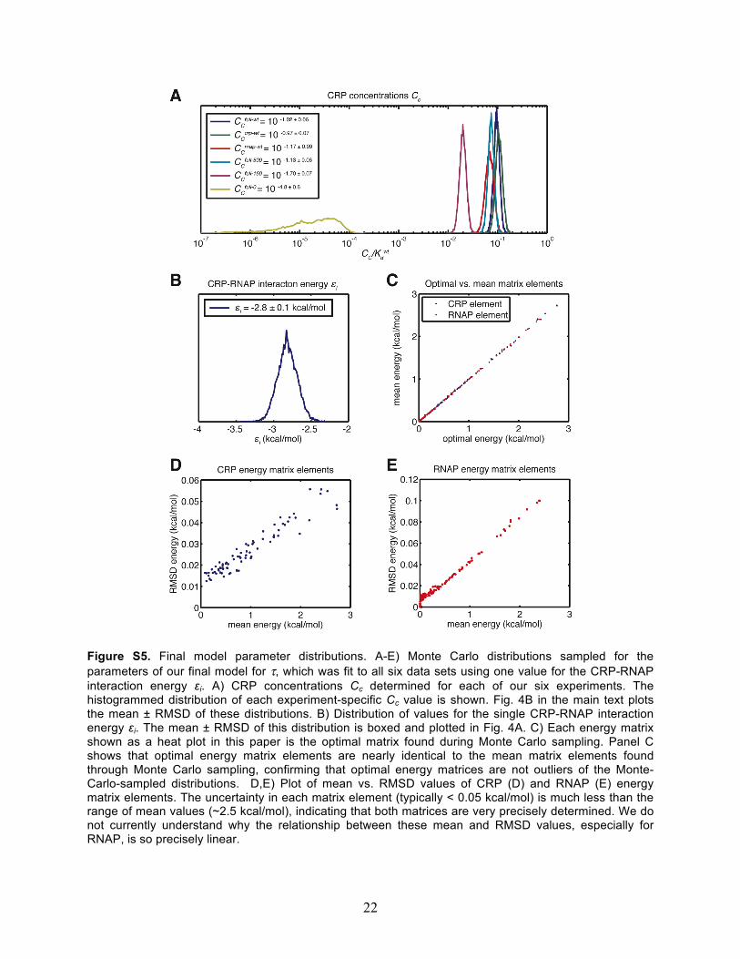
Figure S5. Final model parameter distributions. A-E) Monte Carlo distributions sampled for the parameters of our final model for τ, which was fit to all six data sets using one value for the CRP-RNAP interaction energy εi. A) CRP concentrations Cc determined for each of our six experiments. The histogrammed distribution of each experiment-specific Cc value is shown. Fig. 4B in the main text plots the mean ± RMSD of these distributions. B) Distribution of values for the single CRP-RNAP interaction energy εi. The mean ± RMSD of this distribution is boxed and plotted in Fig. 4A. C) Each energy matrix shown as a heat plot in this paper is the optimal matrix found during Monte Carlo sampling. Panel C shows that optimal energy matrix elements are nearly identical to the mean matrix elements found through Monte Carlo sampling, confirming that optimal energy matrices are not outliers of the Monte-Carlo-sampled distributions. D,E) Plot of mean vs. RMSD values of CRP (D) and RNAP (E) energy matrix elements. The uncertainty in each matrix element (typically < 0.05 kcal/mol) is much less than the range of mean values (~2.5 kcal/mol), indicating that both matrices are very precisely determined. We do not currently understand why the relationship between these mean and RMSD values, especially for RNAP, is so precisely linear.

23

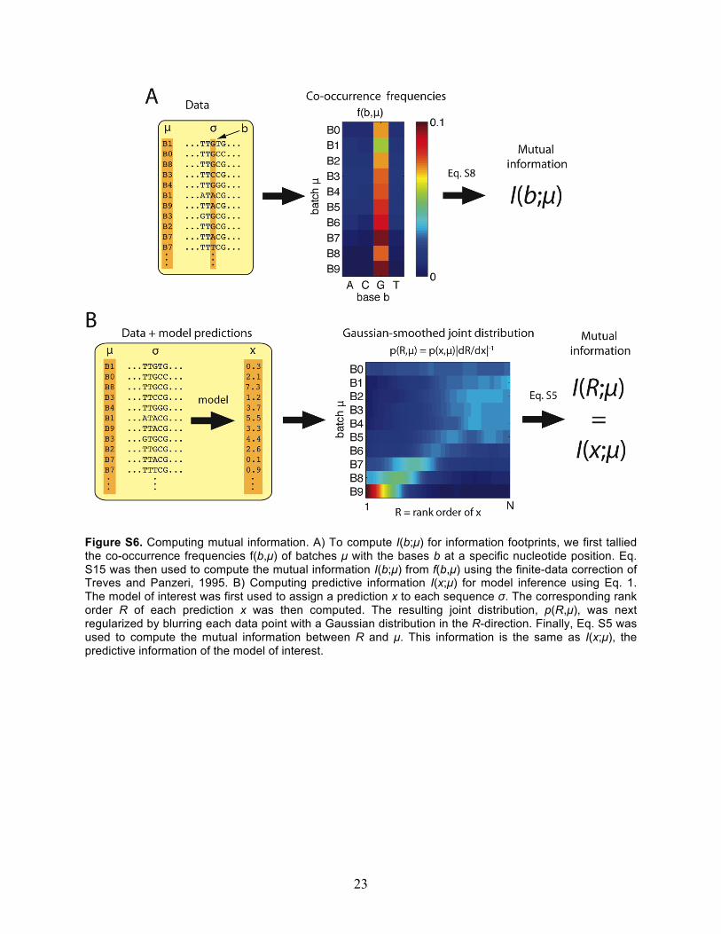
Figure S6. Computing mutual information. A) To compute I(b;µ) for information footprints, we first tallied the co-occurrence frequencies f(b,µ) of batches µ with the bases b at a specific nucleotide position. Eq. S15 was then used to compute the mutual information I(b;µ) from f(b,µ) using the finite-data correction of Treves and Panzeri, 1995. B) Computing predictive information I(x;µ) for model inference using Eq. 1. The model of interest was first used to assign a prediction x to each sequence σ. The corresponding rank order R of each prediction x was then computed. The resulting joint distribution, p(R,µ), was next regularized by blurring each data point with a Gaussian distribution in the R-direction. Finally, Eq. S5 was used to compute the mutual information between R and µ. This information is the same as I(x;µ), the predictive information of the model of interest.

24

Figure S7. Performance of energy matrix models on different data sets. The relative predictive information values of A) 10 different CRP matrices or B) 11 different RNAP matrices are shown for each of the data sets from our six experiments. Each column corresponds to a given set of test data, i.e. data on which I(εc;µ) or I(εr;µ) was computed. In each column, the information value in white text indicates the maximum predictive information (I(εc;µ) or I(εr;µ)) achieved by any of the tested models. Colors indicate the fraction of this maximum value achieved by each of the models tested. Models are annotated along the vertical axis according to the data set they were fit to. Note that some of the energy matrices tested here were inferred directly, while others were inferred as part of a model for τ. In addition, panels A and B each show the performance of three matrix models taken from the literature.