USING COLOUR FEATURES TO CLASSIFY OBJECTS · PDF fileUSING COLOUR FEATURES TO CLASSIFY OBJECTS...
154
USING COLOUR FEATURES TO CLASSIFY OBJECTS AND PEOPLE IN A VIDEO SURVEILLANCE NETWORK By Mathew Price Supervised by Prof. Gerhard De Jager and Dr Fred Nicolls SUBMITTED IN FULFILLMENT OF THE REQUIREMENTS FOR THE DEGREE OF MASTER OF SCIENCE AT UNIVERSITY OF CAPE TOWN CAPE TOWN, SOUTH AFRICA MARCH 31 2004 c Copyright by University of Cape Town, 2004
Transcript of USING COLOUR FEATURES TO CLASSIFY OBJECTS · PDF fileUSING COLOUR FEATURES TO CLASSIFY OBJECTS...

USING COLOUR FEATURES TO CLASSIFY OBJECTS
AND PEOPLE IN A VIDEO SURVEILLANCE NETWORK
By
Mathew Price
Supervised by
Prof. Gerhard De Jager and Dr Fred Nicolls
SUBMITTED IN FULFILLMENT OF THE
REQUIREMENTS FOR THE DEGREE OF
MASTER OF SCIENCE
AT
UNIVERSITY OF CAPE TOWN
CAPE TOWN, SOUTH AFRICA
MARCH 31 2004
c© Copyright by University of Cape Town, 2004

ii

Acknowledgements
This project would not have succeeded without the support of my supervisors, Prof.
Gerhard de Jager and Dr Fred Nicolls (reader extraordinaire). In addition, I would
like to thank TSS Technology (De Beers) and the National Research Foundation for
financial support. Thanks to Bruno Merven (my office neighbour) for the late night
support and my parents for tolerating my anti-social behaviour for the past three
months.
Finally, a huge thank you to Markus ‘legend’ Louw who painstakingly hand-segmented
over 600 frames of video (first two test sequences) so that ground truth measurements
were available.
iii

iv

Abstract
Visual tracking of humans has proved to be an extremely challenging task for com-
puter vision systems. One idea towards the development of these systems is the
incorporation of colour. Often the colour appearance of a person can provide enough
information to identify an object or person in the short-term. However, the imprecise
nature of colour measurements typically encountered in image processing has limited
their use. This thesis presents a system which uses the colour appearances of objects
and people for tracking across multiple camera views in a digital video surveillance
network. A distributed framework for creating and sharing visual information between
several cameras is suggested, including a simple method for generating relative colour
constancy. Tracking has been approached from a classification standpoint allowing
the system to cope with multiple occlusions, variable camera pose, and asynchronous
video feeds. Several test cases exhibiting various surveillance scenarios are used to
assess system performance, which is determined via some well-known surveillance
metrics. The system exhibits an average tracker detection rate of approximately 80%
with a false alarm rate of less than 2%. It is envisaged that the combination of the
presented system and motion estimation tracking techniques could eventually result
in a robust, real-time tracking system.
v

vi

Table of Contents
Acknowledgements iii
Abstract v
Table of Contents vii
List of Tables viii
List of Figures x
1 Introduction 1
1.1 Problem Definition . . . . . . . . . . . . . . . . . . . . . . . . . . . . 2
1.2 Objectives . . . . . . . . . . . . . . . . . . . . . . . . . . . . . . . . . 2
1.3 Layout of document . . . . . . . . . . . . . . . . . . . . . . . . . . . . 3
2 Background 5
2.1 Tracking Approaches . . . . . . . . . . . . . . . . . . . . . . . . . . . 5
2.2 Colour . . . . . . . . . . . . . . . . . . . . . . . . . . . . . . . . . . . 7
2.2.1 Physical Colour . . . . . . . . . . . . . . . . . . . . . . . . . . 7
2.2.2 Human Vision . . . . . . . . . . . . . . . . . . . . . . . . . . . 9
2.2.3 Colour Spaces . . . . . . . . . . . . . . . . . . . . . . . . . . . 11
2.2.4 Colour difference metrics . . . . . . . . . . . . . . . . . . . . . 18
2.3 Clustering . . . . . . . . . . . . . . . . . . . . . . . . . . . . . . . . . 18
2.3.1 Self-Organising Maps . . . . . . . . . . . . . . . . . . . . . . . 19
3 Arch. Overview 21
3.1 Bottom-Up vs Top-Down . . . . . . . . . . . . . . . . . . . . . . . . . 22
3.2 Physical Layout . . . . . . . . . . . . . . . . . . . . . . . . . . . . . . 23
3.3 Data Flow Model . . . . . . . . . . . . . . . . . . . . . . . . . . . . . 24
vii

4 Segmentation 274.1 Motion Segmentation . . . . . . . . . . . . . . . . . . . . . . . . . . . 27
4.1.1 Background Subtraction . . . . . . . . . . . . . . . . . . . . . 284.1.2 Adaptive Pixel Modelling . . . . . . . . . . . . . . . . . . . . 294.1.3 Shadow Removal . . . . . . . . . . . . . . . . . . . . . . . . . 304.1.4 Implementation . . . . . . . . . . . . . . . . . . . . . . . . . . 314.1.5 Limitations . . . . . . . . . . . . . . . . . . . . . . . . . . . . 33
4.2 Colour Segmentation . . . . . . . . . . . . . . . . . . . . . . . . . . . 344.2.1 Pyramid segmentation . . . . . . . . . . . . . . . . . . . . . . 354.2.2 Implementation . . . . . . . . . . . . . . . . . . . . . . . . . . 364.2.3 Limitations . . . . . . . . . . . . . . . . . . . . . . . . . . . . 37
5 Colour Correction 395.1 Colour constancy . . . . . . . . . . . . . . . . . . . . . . . . . . . . . 405.2 Correction using SOMs . . . . . . . . . . . . . . . . . . . . . . . . . . 415.3 Implementation . . . . . . . . . . . . . . . . . . . . . . . . . . . . . . 455.4 Limitations . . . . . . . . . . . . . . . . . . . . . . . . . . . . . . . . 47
6 Object Modelling 496.1 Design Aspects . . . . . . . . . . . . . . . . . . . . . . . . . . . . . . 496.2 Colour Features . . . . . . . . . . . . . . . . . . . . . . . . . . . . . . 516.3 GM Modelling . . . . . . . . . . . . . . . . . . . . . . . . . . . . . . . 53
6.3.1 GMMs versus Histograms . . . . . . . . . . . . . . . . . . . . 536.3.2 Expectation-Maximisation Training . . . . . . . . . . . . . . . 53
6.4 Extended Features . . . . . . . . . . . . . . . . . . . . . . . . . . . . 556.5 Network Synchronisation . . . . . . . . . . . . . . . . . . . . . . . . . 556.6 Implementation . . . . . . . . . . . . . . . . . . . . . . . . . . . . . . 576.7 Limitations . . . . . . . . . . . . . . . . . . . . . . . . . . . . . . . . 59
7 Matching 617.1 Overview . . . . . . . . . . . . . . . . . . . . . . . . . . . . . . . . . . 627.2 Colour Matching . . . . . . . . . . . . . . . . . . . . . . . . . . . . . 637.3 Confidence Measurement . . . . . . . . . . . . . . . . . . . . . . . . . 63
7.3.1 Likelihood Map . . . . . . . . . . . . . . . . . . . . . . . . . . 657.3.2 Quality of colour match . . . . . . . . . . . . . . . . . . . . . 667.3.3 Variety . . . . . . . . . . . . . . . . . . . . . . . . . . . . . . . 677.3.4 Area Distribution . . . . . . . . . . . . . . . . . . . . . . . . . 687.3.5 Proportionality . . . . . . . . . . . . . . . . . . . . . . . . . . 69
7.4 Importance Weighting . . . . . . . . . . . . . . . . . . . . . . . . . . 707.5 Pan Tilt Zoom Extension . . . . . . . . . . . . . . . . . . . . . . . . . 717.6 Implementation . . . . . . . . . . . . . . . . . . . . . . . . . . . . . . 74
viii

7.6.1 Interference filtering . . . . . . . . . . . . . . . . . . . . . . . 757.7 Limitations . . . . . . . . . . . . . . . . . . . . . . . . . . . . . . . . 75
8 Results 798.1 Performance Evaluation . . . . . . . . . . . . . . . . . . . . . . . . . 80
8.1.1 Surveillance Metrics . . . . . . . . . . . . . . . . . . . . . . . 808.1.2 Perceptual Complexity . . . . . . . . . . . . . . . . . . . . . . 818.1.3 Ground truth . . . . . . . . . . . . . . . . . . . . . . . . . . . 83
8.2 Training Parameters . . . . . . . . . . . . . . . . . . . . . . . . . . . 848.2.1 Rough Tuning . . . . . . . . . . . . . . . . . . . . . . . . . . . 858.2.2 Fine Tuning . . . . . . . . . . . . . . . . . . . . . . . . . . . . 858.2.3 Detail sensitivity . . . . . . . . . . . . . . . . . . . . . . . . . 87
8.3 Matching Parameters . . . . . . . . . . . . . . . . . . . . . . . . . . . 898.3.1 Colour matching parameters . . . . . . . . . . . . . . . . . . . 898.3.2 Object matching parameters . . . . . . . . . . . . . . . . . . . 908.3.3 Switches . . . . . . . . . . . . . . . . . . . . . . . . . . . . . . 94
8.4 Test Case 1: Outdoor environment . . . . . . . . . . . . . . . . . . . 968.4.1 Training . . . . . . . . . . . . . . . . . . . . . . . . . . . . . . 978.4.2 Colour correction . . . . . . . . . . . . . . . . . . . . . . . . . 978.4.3 Matching . . . . . . . . . . . . . . . . . . . . . . . . . . . . . 998.4.4 Overall Results . . . . . . . . . . . . . . . . . . . . . . . . . . 100
8.5 Test Case 2: An indoor CCTV system . . . . . . . . . . . . . . . . . 1058.5.1 Training . . . . . . . . . . . . . . . . . . . . . . . . . . . . . . 1068.5.2 Matching . . . . . . . . . . . . . . . . . . . . . . . . . . . . . 1068.5.3 Overall Results . . . . . . . . . . . . . . . . . . . . . . . . . . 108
8.6 Test Case 3: Ceiling cameras . . . . . . . . . . . . . . . . . . . . . . . 1128.6.1 Training . . . . . . . . . . . . . . . . . . . . . . . . . . . . . . 1138.6.2 Colour correction . . . . . . . . . . . . . . . . . . . . . . . . . 1148.6.3 Matching . . . . . . . . . . . . . . . . . . . . . . . . . . . . . 1158.6.4 Overall Results . . . . . . . . . . . . . . . . . . . . . . . . . . 115
8.7 Discussion . . . . . . . . . . . . . . . . . . . . . . . . . . . . . . . . . 1198.7.1 Overall Ratings . . . . . . . . . . . . . . . . . . . . . . . . . . 1198.7.2 Segmentation . . . . . . . . . . . . . . . . . . . . . . . . . . . 1208.7.3 Colour Correction . . . . . . . . . . . . . . . . . . . . . . . . . 1218.7.4 Online Adaptation . . . . . . . . . . . . . . . . . . . . . . . . 121
9 Concluding Remarks 1239.1 System summary . . . . . . . . . . . . . . . . . . . . . . . . . . . . . 1239.2 Future work . . . . . . . . . . . . . . . . . . . . . . . . . . . . . . . . 124
A SOM Training 127
ix

B Test Platform Specifications 129
C Digital Appendix 131
Bibliography 132
x

List of Tables
8.1 Scene Information . . . . . . . . . . . . . . . . . . . . . . . . . . . . 96
8.2 Selected training parameters . . . . . . . . . . . . . . . . . . . . . . . 97
8.3 Colour correction coefficients for Camera 2 . . . . . . . . . . . . . . . 99
8.4 Matching Parameters . . . . . . . . . . . . . . . . . . . . . . . . . . . 100
8.5 Overall test results . . . . . . . . . . . . . . . . . . . . . . . . . . . . 101
8.6 Scene Information . . . . . . . . . . . . . . . . . . . . . . . . . . . . 105
8.7 Selected training parameters . . . . . . . . . . . . . . . . . . . . . . . 106
8.8 Matching Parameters . . . . . . . . . . . . . . . . . . . . . . . . . . . 108
8.9 Overall test results . . . . . . . . . . . . . . . . . . . . . . . . . . . . 108
8.10 Scene Information . . . . . . . . . . . . . . . . . . . . . . . . . . . . 113
8.11 Selected training parameters . . . . . . . . . . . . . . . . . . . . . . . 113
8.12 Colour correction coefficients for Cameras 1, 2 and 3 . . . . . . . . . 114
8.13 Matching Parameters . . . . . . . . . . . . . . . . . . . . . . . . . . . 115
8.14 Overall test results . . . . . . . . . . . . . . . . . . . . . . . . . . . . 116
B.1 Test Platform Specifications . . . . . . . . . . . . . . . . . . . . . . . 129
xi

xii

List of Figures
2.1 Surface colour example. . . . . . . . . . . . . . . . . . . . . . . . . . . 8
2.2 Stage model for human colour perception. . . . . . . . . . . . . . . . . 10
2.3 RGB Cube. . . . . . . . . . . . . . . . . . . . . . . . . . . . . . . . . 12
2.4 HSV hexcone. . . . . . . . . . . . . . . . . . . . . . . . . . . . . . . . 13
2.5 Matching 500 nm wavelength using Newton’s colour circle. . . . . . . 14
2.6 CIE Colour Space w.r.t. RGB cube. . . . . . . . . . . . . . . . . . . . 15
2.7 CIE chromaticity diagram. . . . . . . . . . . . . . . . . . . . . . . . . 15
2.8 CIE L*a*b* colour sphere. . . . . . . . . . . . . . . . . . . . . . . . . 16
2.9 Structure of a Self-Organising Map (SOM). . . . . . . . . . . . . . . . 20
3.1 Ideal System. . . . . . . . . . . . . . . . . . . . . . . . . . . . . . . . 21
3.2 Example of Bottom-Up vs Top-Down systems. . . . . . . . . . . . . . 23
3.3 Distributed Framework. . . . . . . . . . . . . . . . . . . . . . . . . . . 24
3.4 Processing Node Data Flow Diagram. . . . . . . . . . . . . . . . . . . 25
4.1 Segmentation using thresholded background subtraction. . . . . . . . . 28
4.2 Motion segmentation flow diagram. . . . . . . . . . . . . . . . . . . . 32
4.3 Adaptive Background Segmentation with shadow removal. . . . . . . . 33
4.4 Pyramid segmentation process. . . . . . . . . . . . . . . . . . . . . . . 35
4.5 Example of applying pyramid segmentation. . . . . . . . . . . . . . . . 37
5.1 Example of mismatched cameras (Images from VS-PETS 2001) . . . 39
xiii

5.2 RGB clouds for images in Figure 5.1. Red crosses and blue circles
represent the original left- and right-hand side images respectively. . . 43
5.3 SOM prototypes for each RGB cloud shown in Figure 5.2. Red triangles
and blue circles represent the red cross and blue circle classes from
Figure 5.2. Black lines show the translation vectors between each map. 43
5.4 Images before and after SOM processing (top and bottom rows respec-
tively) . . . . . . . . . . . . . . . . . . . . . . . . . . . . . . . . . . . 44
5.5 Camera view comparison after final processing with polynomial smooth-
ing. Second image has been modified to match first image . . . . . . . 46
6.1 POD Training Procedure . . . . . . . . . . . . . . . . . . . . . . . . . 58
7.1 Matching target: Cartman character from South Park cartoon. . . . . 62
7.2 Creation of the likelihood map. Image (a) shows the image divisions;
Graphs (b) and (c) show the 1-D measurement signals in the y and x
directions respectively; and image (d) shows the likelihood map for the
trained character. . . . . . . . . . . . . . . . . . . . . . . . . . . . . . 65
7.3 Variety of object centres across the horizontal image dimension. Object
model colours are shown for positive matches of each centre. . . . . . 68
7.4 Measurement components calculated for Figure 7.2 without impor-
tance weighting. . . . . . . . . . . . . . . . . . . . . . . . . . . . . . . 72
7.5 Measurement components calculated for Figure 7.2 with importance
weighting . . . . . . . . . . . . . . . . . . . . . . . . . . . . . . . . . . 73
7.6 Example frames from a live PTZ tracking sequence. . . . . . . . . . . 74
7.7 Interference filtering example. . . . . . . . . . . . . . . . . . . . . . . 77
8.1 Examples of manually generated ground truth. . . . . . . . . . . . . . 83
8.2 Test characters for training: Stan, Kyle, Cartman, and Kenny (from
left to right). . . . . . . . . . . . . . . . . . . . . . . . . . . . . . . . . 85
xiv

8.3 Tuning training parameters. Each graph shows the results for ktrain = 1
to 4. The number of trained colour classes per character is shown by
the vertical bars and is evaluated for σtrain from 1 to 15. . . . . . . . 86
8.4 Quantisation error between trained classes and actual pixel data versus
the σtrain and ktrain parameters. . . . . . . . . . . . . . . . . . . . . . 86
8.5 Tuning of area threshold. A value of athresh = 2.5 provides a reasonable
estimate to the ideal value for the cartoon characters. . . . . . . . . . 88
8.6 Resulting trained colour classes for each character. . . . . . . . . . . . 88
8.7 Example output of colour matching process. The left hand image shows
the original input, while the right hand image shows which colours have
been matched to character models. . . . . . . . . . . . . . . . . . . . . 90
8.8 Detected object areas for dx = dy taking on values 10, 50, 100 and 200
(divisions from left to right). . . . . . . . . . . . . . . . . . . . . . . . 92
8.9 Object Area Error (OAE) plotted against varying number of divisions. 92
8.10 Left: ROC curve for 50 frames of cartoon sequence for 0 ≤ m1thresh ≤1; Right: Tracker Detection Rate (TRDR) for the same range of m1thresh. 93
8.11 Training Set . . . . . . . . . . . . . . . . . . . . . . . . . . . . . . . . 98
8.12 Trained colour models for training set. . . . . . . . . . . . . . . . . . 98
8.13 Track Detection Rate (TDR) (top); and Object Tracking Error (OTE)
(bottom) for each person. . . . . . . . . . . . . . . . . . . . . . . . . . 101
8.14 Object Model Confusion Matrices . . . . . . . . . . . . . . . . . . . . 102
8.15 Example trajectories for Persons 1 and 2 in Camera 1 . . . . . . . . . 104
8.16 Training Set . . . . . . . . . . . . . . . . . . . . . . . . . . . . . . . . 107
8.17 Trained colour models for training set. . . . . . . . . . . . . . . . . . 107
8.18 (a) Track Detection Rate (TDR); (b) Object Tracking Error (OTE);
(c) Object Model Confusion Matrix . . . . . . . . . . . . . . . . . . . 110
8.19 Example trajectories for Persons 1 (Orange) and 3 (Green) . . . . . . 111
8.20 Training Set . . . . . . . . . . . . . . . . . . . . . . . . . . . . . . . . 114
8.21 Trained colour models for training set. . . . . . . . . . . . . . . . . . 114
xv

8.22 (a),(b) Track Detection Rate (TDR); (c),(d) Object Tracking Error
(OTE) (e),(f) Object Model Confusion Matrix. . . . . . . . . . . . . . 117
8.23 Overall trajectory for Person 2. . . . . . . . . . . . . . . . . . . . . . 118
8.24 Overall TRDR (upper green) and OTE (lower red) ratings for all test
cases. . . . . . . . . . . . . . . . . . . . . . . . . . . . . . . . . . . . . 120
A.1 Updating the Best Matching Unit (BMU) and its neighbours for input
vector x [43]. . . . . . . . . . . . . . . . . . . . . . . . . . . . . . . . 128
xvi

Chapter 1
Introduction
As digital cameras become increasingly small and less expensive, there is a thrust
towards their integration with everyday living. Combined with the processing speeds
of modern computers, many visual tasks previously considered only capable by hu-
mans are now becoming automated. Development of such systems has spawned much
research in the area of machine perception and has been aptly termed — Computer
Vision.
Object tracking is one such area which has drawn a large interest. This is primarily
because of the wide range of applications it encompasses. Some of these include:
detection of stationary objects in airports and train stations (security threats); recog-
nition of human actions; automatic commentary of sports matches; automated person
surveillance for CCTV networks; personal positioning; and vehicle license plate track-
ing.
The context of tracking selected in this thesis applies to the area of computer-aided
surveillance. Large buildings regularly use CCTV networks to monitor the move-
ments of people in order to provide security and safety. This leads to a bottleneck
of information since an operator can only manage a finite number of camera views
accurately at one time. The idea of computer-aided surveillance fits into the interme-
diatory role of filtering out uninteresting events and drawing the operators’ attention
1

1.1. PROBLEM DEFINITION CHAPTER 1. INTRODUCTION
to items of specific importance (eg. people accessing restricted areas). Therefore,
a basic requirement of such a system is the ability to keep track of several people
simultaneously, especially their transitions between different camera views.
1.1 Problem Definition
One interesting problem that arises, is the issue of tracker initialisation. Many predic-
tive tracking techniques have been developed, however, a common weakness in many
of these systems is their dependence on parameter initialisation. Since a prediction is
based on a current assumption and a noisy observation, errors are cumulative and can
lead to eventual target loss. Recovery then requires that the tracker be re-initialised
to the target’s current position. The framework of tracking systems often does not
allow for this.
The system proposed here approaches the tracking problem from a classification
standpoint. Often the colour appearance of a person can provide enough information
to determine their identity and thus their position in the short-term. Therefore, by
modelling this colour appearance as a set of features, colour matching can be used
to build a likelihood response to the model’s spatial position in an arbitrary image.
This one-shot style of tracking has the advantage of being able to deal with occlud-
ing objects, movement between multiple camera views and asynchronous video feeds.
In addition, the framework is extremely flexible, allowing optional integration with a
variety of information such as camera pose, geometric features and motion tendencies.
1.2 Objectives
The primary objective of this work is to determine the limits of using colour infor-
mation in surveillance tracking. It was envisioned that such a system, focusing solely
on visual object features, could then be merged with robust motion estimation tech-
niques to provide a solid tracking framework suitable for use in a large surveillance
2

CHAPTER 1. INTRODUCTION 1.3. LAYOUT OF DOCUMENT
network. These objectives prompted the development of a distributed framework
which can be optimised later for real-time operation.
1.3 Layout of document
This document is structured in a manner that allows the reader to be introduced to
topics in context while preserving the temporal structure of data flow through the
system. For this reason, the Background, Chapter 2, only covers a few global areas.
Further theory for each sub-system is then contained in the introductory sections of
subsequent chapters.
The system framework is introduced in the Architectural Overview, Chapter 3, which
motivates the approach and summarises the system structure and data flow. Each
sub-system is then discussed in Chapters 4, 5, 6 and 7. The arrangement of these
chapters follows a: Descriptive theory; Implementation; and Limitations format. The
descriptive theory systematically derives sub-system concepts while the implementa-
tion and limitations sections describe the realistic customisations specific to coding
and operation.
Results are compiled for three test cases in Chapter 8. Firstly, the assessment
method is described followed by a detailed analysis of the system performance versus
parameter selection. The three test cases are then dealt with separately, concluding
with an overall system performance summary.
Finally, Chapter 9 concludes the document with a brief final overview. The ap-
pendices consist of: An overview of SOM training (Appendix A); a specification
of the test platform used (Appendix B); and a digital appendix (Appendix C)
which refers to the accompanying CDROM. The digital appendix provides the video
sequences for each test case as well as the set of colour trajectory images for each test
subject. The original Acrobat PDF document is also included should any printed
colour diagrams seem unclear.
3

1.3. LAYOUT OF DOCUMENT CHAPTER 1. INTRODUCTION
4

Chapter 2
Background
This project was initiated from the growing need of digital surveillance systems to
perform computer-aided monitoring. Specifically, the idea of classification based on
colour features arose from a previous project in which an on-body camera was used
as a personal positioning device. The variable camera pose and real-time constraints
of that system did not allow conventional methods such as background segmentation
and 3-D pose reconstruction to be applied. This therefore preempted the shift towards
a more featurised and matching-orientated approach.
The work presented in this thesis focuses on fast, reliable recognition of an object
or person’s position in a scene via the matching of colour features. The following
sections aim to provide a broad background within the context of tracking, colour
imaging and data clustering techniques.
2.1 Tracking Approaches
In the global sense, tracking refers to pin-pointing the position of a target object with
respect to some reference at any time. Many different levels of tracking have been
addressed by vision systems, each requiring a different approach. To name but a few:
5

2.1. TRACKING APPROACHES CHAPTER 2. BACKGROUND
Articulate motion: The primary interest here is the accurate recording of a per-
son’s body movements. This has applications in detailed surveillance systems
as well as medical research and automated understanding of body language (eg.
gesture recognition and gait analysis) [34, 20].
Positioning: The aim in a positioning system is to track object positions with re-
spect to their environment. This is classically of interest to the surveillance
community and it represents a very generalised form of tracking.
Detection: Many tracking systems are dependent on the location of a particular
object or body part (eg. animal, box, head, face). Detection methods aim to
provide fast, robust methods for locating such items in an image. These are
normally incorporated into larger systems (eg. [44]).
Robot vision: This arena encompasses a wide variety of methods geared towards
creating autonomous robotic visual systems which mimic human traits. While
the overall tasks are generally simpler (since they must be implemented in stand-
alone hardware), the methods developed are extremely robust and applicable
in a number of other systems (eg. [5]).
In terms of the generalised surveillance tracking class, which is the focus of this thesis,
a number of alternative approaches have been explored. The continual innovation in
this area is attributed to the quest to find the ultimate system which is both robust
and capable of real-time operation.
A well known colour tracking method involves the use of the mean-shift method [7].
This approach uses a histogram-based search which iteratively finds the most similar
target candidate using a histogram similarity metric based on the Bhattacharyya
coefficient. Its primary advantage is its low computational complexity and near real-
time operation. However in the long-term, histogram modelling methods have been
known to fail (even with adaptation). Also, the scaling of models for multiple objects
and camera views is awkward.
6

CHAPTER 2. BACKGROUND 2.2. COLOUR
Motion estimation techniques such as Kalman [45] and particle filters [19] approach
the tracking problem from a stochastic point of view. If objects are parameterised by
their physical interactions with an environment, and these parameters are assumed to
follow a basic motion model corrupted by some noise, then predictive estimates can be
used to track each target’s position in the context of its model. An advantage of this
formulation is that it intuitively facilitates integration with 3-D based information.
Both Kalman and condensation trackers have been applied to solving the multi-view
correspondence tracking problem [27, 28, 30, 49]. However, performance is dependent
on the number of objects and views in the scene as well as the initialisation process.
It is for integration with such systems that this work was aimed.
Simpler approaches such as blob tracking using segmented masks combined with
complex rule sets have also been attempted [25] with some good short-term results.
Solving the problem of computational complexity within high dimensional parameter
spaces, inconsistency of multiple camera hardware, and the lack of a standardised
framework have kept tracking at the forefront of computer vision research.
2.2 Colour
A primary aspect of this thesis is the use of colour matching in digital video. Since the
aim is to create a system that mimics the way humans discriminate objects based on
colour, it is important to understand the underlying processes of human perception
and how it relates to digital imaging.
2.2.1 Physical Colour
The visual spectrum for humans ranges from 400 nm (violet) to 700 nm (red) with a
maximum sensitivity to wavelengths in the 550 nm (green) band [13]. Surfaces appear
coloured as a result of several complex mechanisms which dictate how they transmit,
reflect, absorb and scatter various frequencies of visible light. As a common example,
7

2.2. COLOUR CHAPTER 2. BACKGROUND
the green surface in Figure 2.1 is illuminated by a pure white light source. The surface
absorbs most of the incident frequencies and reflects those in the middle of the visual
spectrum (green). Since an observer looking at the surface will see only the reflected
light, the surface will appear green. Had the illuminating source been pure red, on
the other hand, the surface would have appeared black due to the absence of any
green light for the surface to reflect.
Figure 2.1: Surface colour example.
Generally, surfaces are more complicated than in the illustration. Angles of incidence
and reflection as well as surface shape and material composition play vital roles in
determining the quantities of spectral reflectance. The need to be able to predict
the relationship between incident source light and reflected light on a general surface
has led to the use of Bidirectional Reflectance Distribution Functions (BRDF ). The
amount of light energy travelling in a specified direction, per unit time, per unit area
perpendicular to the direction of propagation, is known as radiance [15]. Its coun-
terpart, irradiance, is defined as the incident power per unit area not foreshortened
[15] (i.e. not perpendicular to the direction of propagation). The BRDF thus charts
the ratio of outgoing radiance to incident irradiance. Simply put, a BRDF maps
the incoming to outgoing direction of light of all visible frequencies for a particular
surface.
In colour imaging, it is convenient to know whether the pixel value represents a true
reading from a surface or whether it has been produced by some sort of lighting
artifact. This knowledge would be especially useful, for instance, if one wanted to
8

CHAPTER 2. BACKGROUND 2.2. COLOUR
normalise the lighting conditions between two images in order to compare object
colours. Since the resulting image is a superposition of many processes, it is not pos-
sible to fully separate each process without extensive analysis of the relevant BRDFs
(assuming they were available). For this reason, a common adopted practice is to
represent the surface as a combination of its Lambertian and Specular components,
which provide a good approximation for a variety of surfaces.
Lambertian or ideal diffuse surfaces describe a special class of surfaces whose re-
flectance is independent of the lighting direction. Examples of such surfaces include
carpets, cotton cloth and matte painted surfaces. A second group of special surfaces
are the specular or mirrored surfaces. Ideal specular surfaces reflect incoming light
about the surface normal at the point of incidence. Generally, ideal specular surfaces
are not overtly common, though many surfaces exhibit specular effects, eg. shiny
metals and plastics. Typically, these surfaces will absorb some light (they are not
perfect reflectors) and cause a variance in the direction of reflection. This produces
a specular lobe or blurring effect. Narrow lobes result in bright specular highlights,
while wider lobes relate to a dull, blurred reflections.
2.2.2 Human Vision
The human sensation of colour has been explained by the receptivity of cone cells in
the retina to a particular frequency of light. Initially it was thought that there were
thousands of types of cone cells, each sensitive to a particular colour, until Thomas
Young introduced the trichromatic model in 1802 [22]. His theory proposed that all
visible colours can be constructed from a mixture of three basic primaries: red; green;
and blue.
Psychophysical experiments conducted by Helmholtz and Maxwell in the mid 19th
century seemed to support Young’s trichromatic representation. The theory was
further confirmed in 1964 when microspectrometry identified the presence of three
types of cone cells [46]: S-Cones; M-Cones and L-Cones (short, medium and long
wavelength). The spectral response of these cones peak at 440 nm (Blue), 545 nm
9

2.2. COLOUR CHAPTER 2. BACKGROUND
(Green) and 565 nm (Red) respectively.
Though trichromatic theory validated the composition of colours via the three pri-
maries, it did not fully explain the abstract process of colour perception. For instance,
the combination of red and green light does not produce a reddish-green as one would
think, but yellow [22]. Another anomaly is the blue after-effect one experiences after
begin subjected to a prolonged yellow stimulus. These effects led to the proposal of
the Opponent Colour theory in 1872 by physiologist Ewald Hering. Hering believed
that there were in fact four unique colours — red, green, blue and yellow — and that
perceived colours were produced by the opponent-processes of three colour channels,
namely red-green, blue-yellow and black-white.
Figure 2.2: Stage model for human colour perception.
The fact that both theories contain truth — trichromatic theory is physically proven
while the opponent colour theory explains the oddities of human perception — has led
to the modern stage theory which combines both representations [22]. Colour vision
is split into two stages as demonstrated in Figure 2.2. The first stage involves physical
reception to an external stimulus by the three types of cone cells in the retina. These
responses are then transformed by a neural process into the opponent colour signals
which are then used for discrimination by the brain. The stage theory is therefore
10

CHAPTER 2. BACKGROUND 2.2. COLOUR
able to explain the trichromatic nature of the human eye while also accounting for
the perceptual sensations humans experience.
2.2.3 Colour Spaces
A linear colour space is a 3-D subspace of co-ordinates that describes a particular
subset (gamut) of visible colours [15]. Colours are matched by the weighted sum
of the three primaries. The weights required in order to match a particular colour
are given by a set of colour matching functions (one for each primary). These colour
matching functions are derived by experimental tuning of the weights of each primary
to match each wavelength of unit radiance in the spectrum [15].
Depending on the application, it is convenient to be able to represent colour data in
various ways. This has led to a vast number of differing colour spaces, each with its
own primaries and colour matching functions.
RGB
Widely used to drive colour CRT displays as well as raster graphic systems, RGB has
become an indispensable device colour system [13]. Colours are represented by the
additive combination of red, green and blue primaries. The R, G, B values generally
range from 0 to 255, forming a cube in cartesian co-ordinates (Figure 2.3). Thus each
colour channel occupies 1 byte or 8 bits in digital media resulting in a 24 bit colour
system.
It is unlikely that RGB image measurements of an object will remain constant over
an extended period. This is primarily due to changes in ambient lighting and environ-
mental positioning. It is therefore convenient to have an invariant which encapsulates
the chromaticity of the object independent of lighting conditions. This introduces the
notion of chromaticity co-ordinates for a colour space, in which the chromaticity is
given by the normalisation of the true values. In RGB, this transformation results
11

2.2. COLOUR CHAPTER 2. BACKGROUND
Figure 2.3: RGB Cube.
in the rgG space where chromaticity is given by the uncapitalised variables r and g,
and G corresponds to the overall intensity. If a pixel has RGB values R, G and B,
the rgG conversion is given by [14]:
r =R
R + G + B(2.1)
g =G
R + G + B(2.2)
G = 0.30R + 0.59G + 0.11B. (2.3)
The b (blue chromaticity) fraction is omitted in rgG, since the normalisation implies
that r + g + b = 1 and therefore the third value can be inferred from the other two.
HSV
In contrast to the RGB space, which is orientated to hardware, the HSV (Hue Satura-
tion Value) model is derived from appearance to users. Closely related to the Munsell
system, HSV uses cylindrical co-ordinates to describe tint, shade and tone [13].
The three perceptual attributes of human colour vision which make up the HSV space
are:
12

CHAPTER 2. BACKGROUND 2.2. COLOUR
Hue: An angle representing the wavelength (colour) of the illuminant. Hue values
range from 0◦ (red) to 120◦ (green) to 240◦ (blue). Complementary colours then
fall uniformly between the primaries (60◦ out of phase).
Saturation: The purity or the radial distance from the unsaturated white point.
The values for saturation span from 0 (white) to 1 (pure Hue).
Value: Sometimes also referred to as Brightness, the Value represents the luminosity
of the colour, which ranges from 0 (black) to 1 (white).
The HSV space thus forms the hexcone depicted in Figure 2.4. Chromaticity in the
HSV space is intrinsically encapsulated by the HS components. However, care must
be taken since Hue is undefined for zero Saturation. This causes noisy chromaticity
measurements in image areas which are excessively bright or dark.
Figure 2.4: HSV hexcone.
CIE XYZ
In 1931, the Commission Internationale d’Elairage (CIE) introduced a representation
which has become the governing standard for colour matching [13]. This representa-
tion was conceived in order to provide a model able to intuitively represent all visible
13

2.2. COLOUR CHAPTER 2. BACKGROUND
colours, thus dealing with the ’negative colours’ phenomenon.
Inconveniently, positive RGB mixtures cannot match the entire range of visible colours
in the spectrum. Newton’s colour circle, shown in Figure 2.5, demonstrates why this
is so, by showing the primaries required to match a 500 nm wavelength[22]. An
additive combination of blue and green will produce a desaturated result. Therefore
in order to match the colour correctly, a negative red stimulus must be added (which
is impossible for CRT devices to achieve).
Figure 2.5: Matching 500 nm wavelength using Newton’s colour circle.
The 1931 CIE XYZ space was therefore devised by defining imaginary primaries X,
Y, and Z so that all visible wavelengths could be matched with positive mixtures.
The transformation from RGB to CIE XYZ maps the RGB cube to the cone-shaped
volume shown in Figure 2.6 by the transformation:
X
Y
Z
=
0.412452 0.357580 0.180423
0.212671 0.715160 0.072169
0.019334 0.119193 0.950227
R
G
B
(2.4)
The CIE chromaticity co-ordinates (x, y, z) [48] are further generated similar to
the rgG transformation (Equation 2.5), forming the xy chromaticity plane shown in
14

CHAPTER 2. BACKGROUND 2.2. COLOUR
Figure 2.6: CIE Colour Space w.r.t. RGB cube.
Figure 2.7.
x =X
X + Y + Z, y =
Y
X + Y + Z, z = 1− x− y (2.5)
Figure 2.7: CIE chromaticity diagram.
A line between points in the CIE chromaticity diagram relates to all available colours
between each endpoint. Furthermore, the colours within a triangle created by three
points in the plane represent the gamut of colours that is available to the set of
primaries defined by the vertices. This means that the CIE XYZ space is intrinsically
15

2.2. COLOUR CHAPTER 2. BACKGROUND
device independent and can be used to compare (or map) gamut regions between
different devices.
CIE L*a*b*
While the CIE xy chromaticity diagram has useful properties for relating gamuts
between various systems, it does not provide a qualitative measure for colour com-
parison. This lead to the definition of several other colour spaces which were geared
to perceptual uniformity.
One of the most successful uniform colour spaces proposed was the 1976 CIE L*a*b*
or CIELAB space [46]. The CIELAB definition is closely related to the opponent
theory of colour vision. Forming a sphere (Figure 2.8), the space consists of two
colour axes a∗ b∗ and a luminance L∗ or brightness axis. The a∗ values range from
red to green, while the b∗ values describe blue to yellow (opponent channels).
Figure 2.8: CIE L*a*b* colour sphere.
The L*, a*, and b* quantities are obtained by a transformation (Equations 2.6 to 2.9)
of the CIE XYZ primaries normalised to a reference white point Xn, Yn, Zn (normally
D65 for general daylight) [46].
16

CHAPTER 2. BACKGROUND 2.2. COLOUR
L* =
{116( Y
Yn)
13 − 16 if Y
Yn> 0.008856
903.3( YYn
)13 − 16 if Y
Yn≤ 0.008856
(2.6)
a* = 500
[f
(X
Xn
)− f
(Y
Yn
)](2.7)
b* = 200
[f
(Y
Yn
)− f
(Z
Zn
)](2.8)
f(t) =
{t
13 if t > 0.008856
7.787t + 16116
if t ≤ 0.008856(2.9)
By definition, a perceptually uniform space means that colour differences between
points in the space are directly proportional to the Euclidean distance measure. Thus
for CIELAB points (L∗1, a∗1, b∗1) and (L∗2, a∗2, b∗2), the difference in colour stimuli
∆E∗ is:
∆E∗2 = (L ∗1 −L∗2)2 + (a ∗1 −a∗2)
2 + (b ∗1 −b∗2)2. (2.10)
If a more descriptive colour difference is required, the suggestion has been to use
the L ∗ C ∗ab H∗ab representation instead [46]. Basically, CIELCH is the polar co-
ordinate equivalent of CIELAB. L∗ remains as the brightness measure, while the
a*-b* plane is replaced by chroma C∗ab (comparable to saturation) and hue compo-
nent H∗ab. The descriptive colour differences between points (L∗1, C∗ab1 , H∗ab1) and
(L∗2, C∗ab2 , H∗ab2) are then given by the three quantities [46]:
∆L∗ = L∗2 − L∗1 (2.11)
∆C∗ = C∗ab2 − C∗ab1 (2.12)
∆H∗ =√
(∆a∗)2 + (∆b∗)2 − (∆C∗)2. (2.13)
where ∆a∗ and ∆b∗ are the component differences in the a*-b* plane.
17

2.3. CLUSTERING CHAPTER 2. BACKGROUND
2.2.4 Colour difference metrics
The nature of an image processing system determines the type of colour model ap-
plied. For instance, an application requiring a descriptive difference between colours
implies that a perceptually uniform colour space should be used.
The previous section described the 1976 CIELAB space which allows the Euclidean
distance between points to be used as a colour difference metric. Unfortunately,
further experiments have proved that CIELAB is not completely uniform [46] and does
not provide a consistently good measure of the magnitude of perceptual difference
between stimuli. This has lead to the definition of other, more optimised metrics
such as CMC (British standard BS:6923), M&S (1980 Marks & Spencer equations
for textile industry), BFD (refined CMC equations), and CIE 94 (simplified CMC
version).
While it has not been proved whether any of these new metrics are better than the
other, the British CMC equation, which uses user-configurable tolerance ellipsoids, is
currently being considered as an ISO standard.
In the context of this thesis, exact colour differences were not critical to operation
(since camera noise distorts image quality in any case). Therefore CIELAB, which is
computationally simpler and more intuitive for spherical feature spaces, was selected.
2.3 Clustering
Discriminative classification methods generally conform to either a supervised or un-
supervised approach [10]. Supervised methods require the structure and pattern of
the presented data to be pre-defined so that the optimum boundaries can be decided.
On the other hand, unsupervised methods are used in order to seek out and discover
the intrinsic patterns for themselves.
18

CHAPTER 2. BACKGROUND 2.3. CLUSTERING
Clustering refers to a set of unsupervised learning algorithms which partition fea-
turised data based on their spatial coherence in the feature space. Clustering meth-
ods are therefore dependent on the separability of pattern features and the type of
distance metric being applied. Two main streams of clustering algorithms exist:
• Partitioning methods
• Hierarchical methods.
Partitioning methods such as K-Means [31], Neural Gas [24] and Self-Organising Maps
(SOMs) [43] operate by dividing the feature space into an optimum set of clusters
which are represented by a set of prototypes. A limitation with many partitioning
methods is their dependency on knowing the number of partitions or pattern groups
n.
Hierarchical methods avoid the specification of n by producing a tree or dendrogram
for all possible divisions according to some similarity metric. An appropriate level
of representation can then be specified by a termination constraint, thus cutting the
tree at some level.
2.3.1 Self-Organising Maps
Self-Organising Maps or SOMs, having a particular application in the colour correc-
tion method presented later, are further discussed. It has been stated that having to
know the number of divisions n limits the unsupervised nature of partitioning clus-
tering schemes. SOMs have the ability to overcome this limitation, thus making them
ideal for analysing completely unknown feature spaces.
A SOM [43], which is essentially a Kohonen Neural Network, is a two-layer network
where the input layer is interconnected to the output layer (as with conventional
neural networks). However, the output layer (competitive layer) is also structured to
form a 2-dimensional grid (shown in Figure 2.9).
19

2.3. CLUSTERING CHAPTER 2. BACKGROUND
Figure 2.9: Structure of a Self-Organising Map (SOM).
During training, each output node is moved so as to be closer to an input vector. In
addition, neighbouring output nodes are also moved towards each other according to
some neighbourhood function. This has the effect of quantising the input vectors, by
folding the grid of neurons around the presented data. Eventually the output grid
becomes an ordered map with similar prototypes close together, thus preserving the
topological structure of the feature space.
SOMs are therefore able to extract the intrinsic patterns of a feature space with their
only constraint being the specified number of training prototypes, which is normally
automatically estimated from the size of the feature space. Features of SOMs include
simple classification (using simple nearest neighbour), dimensionality reduction and
data compression. In addition, hierarchical SOM methods (eg. Growing Hierarchical
SOM [8]) have shown potential in clustering of multi-scale data.
20

Chapter 3
Architectural Overview
The primary goal of the system is to provide a suitable framework for person/object
matching that can be extended over a network of cameras. Since video processing is
extremely resource-hungry, a distributed computing, bottom-up paradigm was chosen
as the basis for this framework. In terms of actual processing, Figure 3.1 encapsulates
the ideal functionality of the system.
Figure 3.1: Ideal System.
21

3.1. BOTTOM-UP VS TOP-DOWN CHAPTER 3. ARCH. OVERVIEW
A camera provides input frames to the Person/Object Detector (referred to subse-
quently as POD). Previously trained colour object models are then used in a matching
process which identifies the location (if any) of the target in the input frame.
3.1 Bottom-Up versus Top-Down
Like many other systems, recognition algorithms can be approached in either a
’bottom-up’ or ’top-down’ methodology [40]. Bottom-up systems are data-driven.
Starting from the input (bottom), subsequent data levels are built upwards by fea-
ture extraction until a level is reached where the features can be compared to the
target model (top).
On the other hand, top-down processes operate in a concept-driven manner. A search
over the parameterised target model (top) yields a predicted view of the target which
is then compared to the actual input. The example shown in Figure 3.2 illustrates
these differences.
The fundamental difference between the two methods is that while bottom-up pro-
cesses build up knowledge from raw data, top-down processes predict lower measure-
ments by assumptions of model coherence. As a result, top-down systems generally
express the entire system as an optimisation problem of measuring the similarity be-
tween a predicted view (based on model parameters) and an observation. This pro-
vides a good representation of the abstraction process, however becomes inefficient
when searching a high dimensional parameter space (common in person/object track-
ing applications) [6]. Consequently, top-down procedures usually require a wealth of
prior information (eg. previous observations, kinematic constraints and camera pose
information) in order to make the parameter search tractable.
Since the POD system is aimed at a fast absolute (no prior information) classification,
a the bottom-up, modularised design was selected.
22

CHAPTER 3. ARCH. OVERVIEW 3.2. PHYSICAL LAYOUT
Figure 3.2: Example of Bottom-Up vs Top-Down systems.
3.2 Physical Layout
The nodes in the distributed framework, shown in Figure 3.3, have been defined by
three primary functions: Processing; Storage; and Management. While the diagram
depicts that each node be allocated its own computer, the framework is intended to be
flexible so that multiple node processes can be economically run on a single machine.
Naturally, this only applies if real-time operation is not a requirement (i.e. off-line
analysis).
Each processing node handles one to two cameras. They are responsible for segmen-
tation, feature extraction, matching and model updates. High-level data, produced
by the processing nodes, is then synchronised with a storage node which provides
global consistency between all nodes.
In terms of the Client/Server model, processing nodes act as hidden servers which
23

3.3. DATA FLOW MODEL CHAPTER 3. ARCH. OVERVIEW
Figure 3.3: Distributed Framework.
serve information to a central point (i.e. storage node). Clients access the high-
level image information from the storage node though a management console. Direct
connections between the management console and processing nodes are also possible
should a live video stream be required. Ideally operators would mainly access the high-
level data streams from the storage node, thus minimising the network transmission
load.
This framework therefore allows a modularised processing approach while preserving
coherence between the multiple data streams.
3.3 Data Flow Model
The processing nodes discussed in the previous section encapsulate the entire func-
tionality of the POD system. The system comprises several pre-processing steps which
24

CHAPTER 3. ARCH. OVERVIEW 3.3. DATA FLOW MODEL
feed into the matching and training processes. A local object model repository pro-
vides the stored features of current targets which are used during matching. Figure
3.4 depicts these operational stages for a single processing node.
Figure 3.4: Processing Node Data Flow Diagram.
The first stage is the digital acquisition of video from a camera. The image is equalised
and filtered for noise using histogram analysis and median filtering respectively.
Following this, three pre-processing steps are used to extract colour features: Motion
Segmentation; Colour Segmentation; and Colour Correction. In order for the match-
ing process to be as fast and effective as possible, it should be presented with as
little irrelevant data as possible. This allows the sensitivity threshold to be increased
without resulting in excess false positive matches. Searching less of the image relates
directly to a faster matching process.
Motion segmentation is used to separate active people and objects from the static
background thus reducing the clutter by a significant amount. Colour segmentation
25

3.3. DATA FLOW MODEL CHAPTER 3. ARCH. OVERVIEW
then groups similar pixel regions, together thus producing a compressed representa-
tion of the motion segmentation. This allows concise models to be constructed and
greatly reduces the computational cost of matching.
When viewing an object with different cameras, it is unlikely that it will appear
identical. Factors such as camera gain, shutter speed and gamma correction can
contribute to large variances in image formation. Additionally, since each camera
will most likely be positioned differently (probably in different rooms), environmental
lighting conditions will also cause inconsistency between views. Since the system must
be able to compare a person or object’s colour between views, a method of calibrating
all cameras to a common colour subspace is necessary. Towards this end, the colour
correction stage uses trained samples of a camera’s response to a range of colours in
order to calculate an appropriate adjustment.
The features produced by the pre-processing stages are represented by a cluster of
colour centres. They are then applied to the core of the system. Initially, since the
object model repository will be empty, the training stage will use the features of a
specific target to discover the best representation for that target. This trained feature
set is then added to the object model repository.
Once trained object models are available, the matching process is activated and pro-
duces a likelihood response to the existence of each target listed in the local repository.
Close matches are processed through an adaptation stage and used to incrementally
update the stored models. This allows the system to track gradual drifts caused by
lighting artifacts. Information about each matched target is compiled into a running
profile and stored. Finally, the likelihood outputs can be combined, and together
with the input image produce a labelled image of the position of any visible targets.
The next four chapters provide a break-down of each processing stage.
26

Chapter 4
Segmentation
Segmentation is the process of extracting relevant information from an input data
stream for a specific application. In visual tracking, segmentation normally refers to
automatically separating a desired object or person from a background scene. While
ideally the segmented foreground image should contain all the pixels relevant to its
target, in reality this entity is extremely difficult to define.
In the POD system, segmentation is a pre-processing step thus requiring it to be
optimised for speed. A simple two-part segmentation scheme is used for reducing
clutter and extracting colour features from objects. Firstly, motion segmentation by
way of background subtraction removes target candidates from the static background
scene. The next step involves a colour segmentation process whereby regions of similar
colour in the foreground are grouped together and represented by a cluster of colour
centres. This reduces the load on the training and matching stages, and provides a
concise object description system capable of being synchronised over a network.
4.1 Motion Segmentation
Owing to the fact that model training focuses only on significantly large and consis-
tent colour regions of the foreground object, exact segmentation was not a priority.
27

4.1. MOTION SEGMENTATION CHAPTER 4. SEGMENTATION
Therefore a simple adaptive background subtraction algorithm was used.
4.1.1 Background Subtraction
Essentially, background subtraction operates by taking a frame BG containing only
the static background, and subtracting a consecutive frame P from it. Any pixel
difference which deviates more than a set threshold Tdiff is considered foreground
(shown in Equation 4.1). In this way a foreground mask M can be obtained:
M(x,y) =
{1 if |P(x,y) −BG(x,y)| > Tdiff
0 otherwise(4.1)
In reality, thresholding all pixels in the image by the same amount does not provide
reliable results, as demonstrated in Figure 4.1.
Figure 4.1: Segmentation using thresholded background subtraction.
Factors such as light distribution and colour differences can cause inconsistencies
in the comparison between foreground and background pixels. Additionally, it is
unlikely that the background will remain entirely static due to persons interacting
with furniture and objects. Also, shadows cast by foreground objects may cause
background to be regarded as foreground. Therefore, realising a segmentor that can
cope with such problems led to two useful strategies:
28

CHAPTER 4. SEGMENTATION 4.1. MOTION SEGMENTATION
1. Adaptive Pixel Modelling
2. Shadow Removal.
4.1.2 Adaptive Pixel Modelling
An alternative to using a global threshold for the subtraction is to assume that each
pixel deviates according to its own model, and thus to threshold each pixel in the
context of its model [41]. For simplicity and speed, a unimodal normal distribution
was used here.
If each pixel is assumed to vary with a normal distribution over time, then it can
be represented by a mean µ(x,y) and a variance σ2(x,y) (assuming a single channel,
grayscale image). A background model BG can then be adaptively updated from
consecutive input frames P as suggested by [25]:
µBG(x,y)(t + 1) = (1− α)µBG(x,y)
(t) + (α)µP(x,y)(t + 1) (4.2)
σ2BG(x,y)
(t + 1) = (1− α)σ2BG(x,y)
(t) + (α)σ2P(x,y)
(t + 1), (4.3)
where (0 ≤ α ≤ 1) and controls the rate of adaptation. Typically, a high value for α
is used to initialise the model after which the value is lowered so that the model does
not adapt to foreground motion. An α of approximately 0.05 was found to provide a
good balance, allowing the system to cope with slow, variations in lighting. Although
small, repetitive motion of small regions can produce jitter which does not conform
to the unimodal normal distribution [35] (eg. leaves swaying in wind), these areas are
usually small and isolated and can be filtered out by morphological processing.
Each pixel in the input frame P is then assumed to be part of the foreground mask
M if it meets the condition:
|P(x,y) − µBG(x,y)| > max(kσBG(x,y)
, nCCD). (4.4)
The constant k determines the threshold and is typically 3 while nCCD, representing
the camera’s internal CCD noise, ensures that σ2 does not become too close to zero.
29

4.1. MOTION SEGMENTATION CHAPTER 4. SEGMENTATION
This procedure can then be applied to colour images by simply modelling and adapt-
ing each colour channel’s mean and variance separately (i.e. µR(x,y), µG(x,y), µB(x,y)
and σ2R(x,y), σ2
G(x,y), σ2B(x,y)).
4.1.3 Shadow Removal
The second artifact which can cause inaccurate segmentation is the interaction of
shadows. When a moving person or object casts a shadow over the background
model, the covered pixels become darker and can exceed the adaptive threshold thus
causing them to be incorrectly associated with the foreground.
Approaches to shadow reduction range from approximation using models to adaptive
thresholding and chromatic analysis. A popular method is to notice that shadows
cause a reduction of lightness over the covered region without affecting the chro-
maticity (hue and saturation) [25]. Therefore, certain shadows can be removed by
modelling the background in chromaticity co-ordinates such as CIE xy, rgG, etc1.
Unfortunately, while in practice this removes shadows, discarding the luminance in-
formation can lead to instability [21] since any true foreground areas whose chro-
maticity matches the corresponding background model will be erroneously classified
as shadow (eg. a green shirt in front of grass).
A compromise is reached by using first-order gradient information to detect shadows
with soft edges as proposed by [25]. When an object has similar chromaticity to
its background, its gradient image will differ depending on the textural differences
between the two. Therefore the foreground is detected by the differential change of
either the chromaticity or gradient models. One downfall is that the method is can
only deal with soft-edged shadows (which are common). Strong shadow edges (areas
of large contrast) will produce a large gradient differential and therefore be incor-
rectly labelled as foreground. The gradient model, as stipulated by [25], comprises
of three gradient means (µxr, µyr), (µxg, µyg), (µxb, µyb) (one for each RGB channel)
1Colour spaces are discussed in Section 2.2.3.
30

CHAPTER 4. SEGMENTATION 4.1. MOTION SEGMENTATION
and corresponding magnitude variances σ2gr, σ2
gg, σ2gb. Gradients are constructed by
convolving each image channel with the Sobel X and Y operators. Pixels are then
adapted and thresholded in exactly the same manner as discussed in the previous
section (see Equations 4.2 and 4.4).
In order to improve the process, CIE L*a*b* co-ordinates are used in place of RGB
(on account of their better pixel differences). Further, by only creating gradient mod-
els for the L* (intensity) channel, the nine parameters (originally six RGB gradient
means and three variances) are reduced to three, i.e. (µxL∗, µyL∗) and σ2gL∗ (gradi-
ent mean requires two parameters — x and y components). Although this reduces
the sensitivity of the gradient measure between different colours, it provides a man-
ageable model that can operate close to real-time and therefore not hinder system
performance.
4.1.4 Implementation
The combination of the modelling and shadow removal forms a robust basis for the
motion segmentor. The final background pixel model is a function of six parame-
ters, BGx,y(µa∗, µb∗, µxL∗, µyL∗, σ2a∗b∗, σ
2gL∗), where co-ordinates are described in the
CIELAB colour space and the chromaticity variance is calculated as the magnitude
of the difference in the a*-b* plane. A foreground mask is thus extracted from an
input frame via the process shown in Figure 4.2.
After converting to CIELAB, x and y first-order Sobel gradients are constructed. The
sum of the squared difference between the gradient images and their corresponding
model means (µxL∗, µxL∗) is then calculated and compared with the gradient magni-
tude variance model (σ2gL∗). Similarly, a chromaticity magnitude image is calculated
and compared with the chromaticity variance model (σ2a∗b∗). An initial foreground
mask is thus constructed by combining the two results.
The intermediatory foreground mask now consists of large foreground objects and
many small uncertainties. Assuming that true foreground objects (eg. people) will
31

4.1. MOTION SEGMENTATION CHAPTER 4. SEGMENTATION
Figure 4.2: Motion segmentation flow diagram.
32

CHAPTER 4. SEGMENTATION 4.1. MOTION SEGMENTATION
occupy a minimum blob (connected component) area, morphological opening is used
to remove isolated pixel noise. This is followed by a minimum area thresholding
procedure which also fills in isolated holes inside object masks should they be less
than a filling area threshold. The area thresholding process also constructs an up-
date mask used to determine which areas of the image should not be included in
updating the background model (i.e. any probable foreground). Once completed, a
morphological closing ensures that object edges are restored from the original opening
function. Since the small, noisy areas have already been filtered out, only the remain-
ing foreground objects are affected. The end result is a binary foreground mask which
identifies any significant motion. An example of the result is shown in Figure 4.3.
Figure 4.3: Adaptive Background Segmentation with shadow removal.
4.1.5 Limitations
Background subtraction is limited to use with static, fixed cameras due to the nature
of the subtraction (so that the background image stays the same). The process also
requires that the initial model be trained without any potential foreground objects
— otherwise the background model would learn these.
The fact that the POD system uses the segmentation simply as a load reducing
filter allows these limitations to be less restrictive. Firstly, moving the camera will
33

4.2. COLOUR SEGMENTATION CHAPTER 4. SEGMENTATION
simply produce more foreground regions which need to be searched. The initial-
training limitation can also be overcome by adding the matched objects of a first
unsegmented frame to the update mask, thereby stopping the initial adaptation from
including these objects in the background model. This obviously implies that the
object models are known beforehand and therefore the initial object modelling process
must use images from a static camera.
4.2 Colour Segmentation
A typical 352 × 288 image contains over 100 000 pixels. Since it is desired to train
models relating to distinguishable coloured areas of an object, it would make sense
not to have to process every pixel in order to determine its colour grouping. Therefore
a batch colour segmentation method allows an efficient quantisation of the foreground
into coloured components, leading to a more compressed data representation which
is better suited to higher-level processing. As colour segmentation applies to the
training of object colour models, the process operates on the segmented foreground
mask produced by motion segmentation.
Region-based segmentation has been a particular interest in image content-based
retrieval databases where, a huge number of images must be searched for feature
matches. The compact nature of segmented images allows for more generalised and
faster searching. In contrast to the motion segmentation process, region-based meth-
ods are normally localised to the similarity of regions within a single image. Some
techniques which are conventionally applied to the problem include: optimised am-
plitude thresholding [31]; recursive region growing [1]; K-Means clustering [31]; and
vector field analysis [42].
Preliminary comparative testing performed by [23] towards the goal of fast, automated
segmentation showed that multiscale processing methods are the most appropriate
when speed optimisation is a requirement. This confirmed our findings that the use
of pyramid segmentation by way Gaussian pyramid decomposition was an efficient
34

CHAPTER 4. SEGMENTATION 4.2. COLOUR SEGMENTATION
mechanism for the colour segmentation process.
4.2.1 Pyramid segmentation
Multiscale image processing techniques are hierarchical processes which use multiple
resolutions of an image to perform analysis. These can be approached as top-down
(quad-tree decomposition) or bottom-up processes (image pyramids). In the latter
methods, image levels are constructed by downsampling the image by a series of filters
— Gaussian in this case — which provides a smoother output.
The OpenCV library [18] provides a well optimised implementation based on the
algorithm proposed in [6]. The input image (largest) can be thought of as the base of
the pyramid. Each consecutive level is then built upwards, downsampling by a factor
of two at each stage, until a specified maximum level is reached (commonly between
3 and 5). Two thresholds, T1 and T2, determine the nature of the segmentation, and
linking is performed in two stages illustrated in Figure 4.4.
Figure 4.4: Pyramid segmentation process.
1. A link between a pixel px,y on level L and its candidate father p′x′,y′ on level
35

4.2. COLOUR SEGMENTATION CHAPTER 4. SEGMENTATION
L + 1 is established if: dist(c(px,y, L), c(p′x′,y′ , L + 1)) ≤ T1.
2. Connected components A and B are then clustered together if: dist(c(A), c(B)) ≤T2.
The function dist is the Euclidean distance between local property functions c for each
pixel. The local property c is the type of measurement associated with a pixel, which
in this case c is simply the intensity of the pixel. Therefore, the distance calculated by
the dist function is effectively the difference in pixel intensities |i(x, y)− i(x′, y′)|. For
colour images, the intensity is calculated by the weighted grayscale approximation:
|iRGB(x, y)− iRGB(x′, y′)| = 0.30|iR(x, y)− iR(x′, y′)|+ (4.5)
0.59|iG(x, y)− iG(x′, y′)|+
0.11|iB(x, y)− iB(x′, y′)|.
4.2.2 Implementation
As previously mentioned, the pyramid segmentation scheme from the Intel OpenCV
library was used for the system’s colour segmentation. The fact that this method pro-
duces connected components which are not necessarily spatially linked (global clus-
tering) led to a minor post-processing modification. This involves scanning through
the list of presented regions and splitting unconnected components having the same
label into a separate region. Further, a lower-bound area threshold (10 pixels) was set
in order to stop noisy one- and two-pixel regions from being submitted as features.
Parameter tuning, which is the thrust of [23], was found to be fairly inconsequential.
Unlike [23], the primary goal was to reduce the mass of pixel data to a manageable
number of classes (approximately 5% of the image pixels). Therefore exact parameters
for maximising the quantisation was not required. In fact, a larger list of small regions
which more accurately describe the original pixel colours is preferred. In general,
setting T1 = 30 and T2 = 10 provided equitable results. Figure 4.5 shows an example
output.
36

CHAPTER 4. SEGMENTATION 4.2. COLOUR SEGMENTATION
Figure 4.5: Example of applying pyramid segmentation.
4.2.3 Limitations
The only inherent limitation of the pyramid segmentation method is its tendency to
merge unrelated colours if the thresholds are set too high. Since the POD system
does not require an optimised minimum set of clusters, fixing the thresholds at the
previously suggested values ensures that high definition separation is maintained.
One other minor artifact involves the size of the input image. Since downsampling
requires image dimensions which are divisible by two, the input image must be padded
so that it can be downscaled a number of times.
37

4.2. COLOUR SEGMENTATION CHAPTER 4. SEGMENTATION
38

Chapter 5
Colour Correction
One of the primary requirements of a multi-camera colour tracking system is consis-
tency of colour measurements between several cameras. Colour constancy refers to
the correction of colour deviations caused by a difference in illumination [47]. Failure
of the system to provide a correlation between similar colours over the camera network
would cause colour-based appearance models to become invalid once a person leaves
the view of any camera. Figure 5.1 shows an example of two unmatched surveillance
cameras.
Figure 5.1: Example of mismatched cameras (Images from VS-PETS 2001)
39

5.1. COLOUR CONSTANCY CHAPTER 5. COLOUR CORRECTION
5.1 Colour constancy approaches
The problem of colour constancy has been under scrutiny for some time in the image
retrieval area, where the classification of images is sometimes reliant on the similarity
of colours. The general trend is to find an illumination invariant transform from the
usual RGB pixel representation, which provides consistent measurements irrespective
of the illumination direction, surface orientation and intensity. Examples of such
transforms include normalised RGB (rg) and HS (Hue-Saturation), which provide
good colour invariants under white light [3]. However, in a real camera environment,
lighting configurations will cause different camera hardware to measure different hues
(device dependent colour spaces), thereby invalidating any such invariant. This means
that before such information is to be of any use, the dynamic ranges of the contrasting
images must be normalised. Methods for achieving colour constancy generally fall into
one of three groups:
Physical Modelling: These methods involve formulating an invariant by analytical
derivation of spectral image formation from its physical processes. Since lighting
models are extremely complex, many assumptions and generalisations are made
about the scene in order to isolate the primary processes. An example is the
work presented by Geusebroek et al. in [16], which deals with finding a colour
invariant for scenes in which the illumination colour changes over time.
Human Vision Modelling: Here processes are modelled after the human visual
system, which tries to maximise image dynamics while perceptually normalis-
ing the scene information. Several illumination adaptive mechanisms, which are
attributed to low-level eye functions, have been explored in image processing.
One such mechanism is the hypothetical White Patch reference. This normalises
the colour channels towards an ideal white point reference. Another mechanism,
known as Gray World, involves adapting the image dynamics so that they fall
within a comparable range. This relates directly to matching image dynamics
by performing a type of mean-level adjustment. A combination of such mech-
anisms, as in [33] and [32], has proved viable towards performing unsupervised
40

CHAPTER 5. COLOUR CORRECTION 5.2. CORRECTION USING SOMS
colour correction.
Model Normalisation: By assuming a generalised lighting model (eg. Lambertian
or Specular Reflection), the entire illumination process can be broken into a se-
ries of transforms. Unwanted components can therefore be removed (by making
certain assumptions) and thus result in an invariant set of colour co-ordinates.
While this seems similar to the Physical Modelling methods, the difference lies
in the assumptions, which use models of human visual responses and not exact
physical processes. These methods therefore bridge the previous two groups.
An example is the work of Finlayson and Xu [12], which uses the log RGB space
for colour normalisation. They derive pixel colour using a Lambertian lighting
model and scale the channel means using Gray World normalisation. The bene-
fit of using log RGB space is that products become sums and therefore removal
of components can be achieved by a simple subtraction. Most importantly
though, device gamma (which is a power function) can be cancelled out using
logs. This is extremely useful when comparing images from different cameras.
5.2 Unsupervised colour correction using SOMs
In light of the fact that our system is geared towards near real-time operation, it
follows that a fast, robust colour constancy method is needed. Since we are using
multiple cameras, the method must be insensitive to camera pose and position in
addition to the usual invariants. The Video-CRM system described in [17], which has
similar requirements, proposes the use of a colour calibration target. The basic idea
is to show the calibration target to each camera and use the responses to calculate
the gamut mapping between the two image systems.
In a large camera network, however, it is desirable to have a more automated approach
which does not encumber the users. In any case, mapping based on a target can
never be totally accurate unless it takes into account colour or intensity shifts within
a single image frame. This would require the calibration target to be evaluated at
41

5.2. CORRECTION USING SOMS CHAPTER 5. COLOUR CORRECTION
several positions for each view, leading to a lengthy calibration procedure.
Austermeier et al. [2] have shown a useful method for performing an unsupervised,
target-based calibration scheme for normalising illumination changes. Their tests
showed that a cloud of RGB pixels (plotted by omitting their spatial image placement)
preserves its topology when subjected to a change in illumination. Furthermore, if
the clouds of the original and resulting images are each quantised by a set of SOM
prototypes1, pixel colour can be corrected by simply translating its prototype between
the two maps. SOMs have the useful feature of being able to quantise data into a set
of prototypes, while at the same time preserving topological relationships between
neighbouring neurons.
To clarify, usually the main usage of SOMs is for dimension reduction of feature
data. However, in this application it is simply used as a 3-D data-fitting method.
Another common practice is to use a 2-D neuron grid for the SOM. The main reason
is because its distance matrix (depicting clustering information) is best understood
in planar form. Once again, since this scheme is using the SOM’s fitting ability, it is
necessary to use an exact representation of the data, and thus the map is created as
a 3-D lattice.
As an example, consider the two camera views presented previously in Figure 5.1.
Figure 5.2 shows a plot of RGB clouds for each image. As expected, the brighter left-
hand side image (red crosses) has a greater dynamic range, indicated by the larger
RGB values.
If the clouds are now quantised into two 3-D SOMs, the original pixels can now be
represented as a reduced set of prototypes (Figure 5.3). The most important factor
is that each SOM must be identically, linearly initialised before being adapted to a
data cloud. This creates an intrinsic mapping link between corresponding prototypes
and allows inter-SOM mapping by simply calculating translation vectors for each
prototype. Using this idea — namely that neighbourhoods of pixels can be mapped
to a reference — all that is required is a set of translation vectors defined for each
1SOMs are reviewed in Section 2.3.1 and the training procedure is outlined in Appendix A.
42
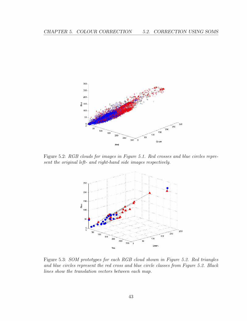
CHAPTER 5. COLOUR CORRECTION 5.2. CORRECTION USING SOMS
Figure 5.2: RGB clouds for images in Figure 5.1. Red crosses and blue circles repre-sent the original left- and right-hand side images respectively.
Figure 5.3: SOM prototypes for each RGB cloud shown in Figure 5.2. Red trianglesand blue circles represent the red cross and blue circle classes from Figure 5.2. Blacklines show the translation vectors between each map.
43

5.2. CORRECTION USING SOMS CHAPTER 5. COLOUR CORRECTION
neighbourhood. These are indicated by the black connecting lines in Figure 5.3.
As seen in the above figure, the SOM not only compresses the data representation, but
also provides the translational relationships between pixel neighbourhoods between
images. Therefore, once the pixels in the darker image (blue class) are translated by
the SOM vectors (black lines), image balance is improved. The result of correcting
the second image with respect to the first image is shown in Figure 5.4. Owing to the
quantisation process the output image lacks smoothness. However, if the CIELAB
co-ordinates of similar surfaces are compared between the unmatched views (eg. the
grass and road areas), it is found that colours in the corrected image are on average
two times closer than the uncorrected image (using CIELAB distances).
Figure 5.4: Images before and after SOM processing (top and bottom rows respectively)
44

CHAPTER 5. COLOUR CORRECTION 5.3. IMPLEMENTATION
5.3 Implementation
The colour correction process in the system flow diagram in Figure 3.4 (Chapter 3)
is shown to follow the colour segmentation stage. This is because correcting fewer
pixels is faster, and because only the segmented targets need to be corrected in order
for model colour matching to succeed. Training of the colour correction mappings,
however, operates directly on the input images.
There are some problems with the SOM method proposed by [2]. Firstly, they rec-
ommend training the image pixels using a 25×25×25 SOM grid. SOM training time
tends to follow an exponential trend as the map size increases. Additionally, the size
of the set of input data also contributes to the number of training steps and amount
of memory required.
Since it was not tractable to follow the suggested parameters, it was decided to pre-
quantise the pixel data into similar classes in order to reduce the amount of data
being presented to the SOM. The natural choice was to use the existing pyramid
segmentation2 scheme which retains the major colour groups. While this reduced the
computation significantly, memory resources still restricted the map size to a level
that could not adequately represent the data.
The second modification was therefore to split the input data into several batches and
to train a small SOM (5×5×5) for each batch. Once complete, all the SOM prototypes
could be recombined and used per normal. For the splitting process to work, it was
important to retain coherence between each image’s prototypes so that the SOM’s
topological information would remain intact. Thus, in place of training a SOM for
each image part, a single SOM was trained to the first input and then adapted to
the second. Finally, it was found that using CIELAB co-ordinates in place of RGB
provided better results, since CIELAB space produces a smaller distance error3 when
quantising colour values.
2Details given in Section 4.2.3Intrinsically, colour perception in CIELAB is supposed to be directly proportional to Euclidean
distance.
45

5.3. IMPLEMENTATION CHAPTER 5. COLOUR CORRECTION
The type of correction warranted by the POD system generally requires that the
general image trends be the same for a comparison. In order to provide a smoother
overall response for correction, a linear least squares fit of the input-output prototype
map is used as a post-processing step. The colour correction coefficients are calculated
in the RGB space resulting in a fast mapping between camera views. Equation 5.1
shows the correction from pixel R,G,B to R′, G′, B′:R′
G′
B′
1
=
xR 0 0 x0
R
0 xG 0 x0G
0 0 xB x0B
0 0 0 1
R
G
B
1
(5.1)
The result of the final implementation is shown in Figure 5.5 using the same images
from the previous example. The smoother response in the corrected image is evident
and the perceptual colour difference between the unmatched views (using CIELAB
distances) is now nearly three times closer for the corrected image.
Figure 5.5: Camera view comparison after final processing with polynomial smoothing.Second image has been modified to match first image
46

CHAPTER 5. COLOUR CORRECTION 5.4. LIMITATIONS
5.4 Limitations
A fundamental difference between the application of colour constancy in our system,
as opposed to other contemporary work, is that we try to normalise the colour system
between two different camera systems. Most results of colour constancy algorithms
use computer-generated scenes as their basis for trials. While this proves that the
algorithm can correct for artifacts matching the models used to create the scene, it
rarely relates to the unpredictable nature of real camera views. Keeping this and the
requirements of our system in mind, the colour correction implementation developed
was tailored to improving the comparison of CIELAB colours between camera views,
and not providing an ideal transformation.
A common problem is caused by extremely bright or excessively dark regions. Though
the camera provides a non-linear output voltage from the CCD, the camera response
is still limited to its range (dictated by the aperture setting, shutter speed and gain).
Therefore without being able to dynamically modify camera parameters, a digital
image processing system cannot recover information which has fallen outside the
range. Simply put, if the image values saturate at either 0 or 255 (RGB sensor
limits), it is generally not possible to determine the true colour of the pixel. In colour
constancy, this means that for two different camera views, there are only two possible
adjustments:
1. Normalising the dynamic range
2. Adjusting data within the dynamic range of the image.
The unsupervised nature of the method relies on the fact that similar, but distorted,
colour classes exist in both images. Therefore the system is limited to correcting
scenes which have similar environmental colours. Should varying environments need
to be matched, a calibration target or known object must be present in each scene in
order to determine the general difference. This could be achieved by having a person
wearing a suitably coloured jacket traverse the various camera areas. All failing, a
47

5.4. LIMITATIONS CHAPTER 5. COLOUR CORRECTION
final alternative is for the system to ask a user to manually specify matching colours
between scenes using a pixel selection tool.
48

Chapter 6
Object Modelling and Training
At first, it was hoped that a full unsupervised training method would be achievable by
the analysis and filtering of the segmented images. The original idea was to determine
the presence of a single person or object from the segmented mask by observing the
tendencies of certain colours to move together on average.
Ultimately, it was decided that this process could best be implemented in the future,
after a solid matching process (the primary objective of the thesis) was established.
This resulted in a semi-supervised training process which self-determines the ‘best’
colour features corresponding to a target, given the set of features from several images
of that target.
6.1 Design Aspects
What makes an object visually distinguishable from its background? Commonly, this
tends to be a combination of: geometric shape and size; texture and colour; and prior
knowledge about its environmental likelihoods (for instance, trees tend to be situated
49

6.1. DESIGN ASPECTS CHAPTER 6. OBJECT MODELLING
outside).
In particular, humans make extensive use of colour in recognition. This is probably
due to the virtually instantaneous nature of colour information. For instance, someone
describing a car would normally note its colour before its make or model. This means
that once a target has been identified, short-term (and sometimes long-term) tracking
can be maintained by colour matching. Of course this process does rely on the fact
that the target’s colour appearance is suitably distinguishable from its background.
With regards to the POD system, the aim was for training to accept input samples
from either a user-selected area or a motion-segmented data stream (controlled by
the matching process). Since training samples for an online system are sparse, it was
further decided to design a modelling process which can create a reasonable object
representation based on a single observation. Additional observations are then used
to refine the model. The result is a training method which operates by filtering the
segmented colour features based on the following criteria:
• Which colours are chromatically most distinctive?
• What are the general proportions of each colour?
• On average, which colours are most visible?
• How well is each colour matched between training steps?
Most of the time, colour is an extremely meaningful descriptor of an object, eg. blue
sky, pink skin, brown hair. Other times, it can provide incorrect or no information
at all, eg. dark areas, oddly lit environments. The fact that colour is not totally
infallible suggests that machine vision trackers should, like humans, employ a variety
of different types of features.
There are three main reasons why other visual features were not incorporated into
this project. The first was based on a desire to find the limitations of using colour in a
machine vision system. Colour comparisons in digital imaging have proved extremely
50

CHAPTER 6. OBJECT MODELLING 6.2. COLOUR FEATURES
challenging due to camera and capture hardware limitations and variations. Secondly,
the system was designed with the intention of working in conjunction with other
estimation techniques. This implied that focus should be centred on the neglected
areas of those systems and thereby a combined system would be able to exploit the
strengths of both processes. Finally, since the project tackles the problem from a
feature classification standpoint, the framework easily allows for future incorporation
of additional features with little modification.
A common problem with training methods is their tendency to focus on the process of
creating a descriptive model of the data and ignoring its accessibility to the matching
process. This means that while analysis of each trained model provides a good high-
level representation of that object, comparisons between object models are limited by
the efficiency of the matching process and its associated distance metrics.
An example of this is an object which is modelled by several histograms. While the
histograms may encapsulate the object’s tendencies, it does not account for the fact
that many histogram comparison methods do not provide consistently reliable results.
Additionally, the presence of multiple object models would require an exhaustive
search thereby impeding the hope of a near real-time system.
The development of the POD training process was therefore preceded by design of an
efficient matching process. This was then followed by an analysis of how matching
could be improved by affecting the training process.
6.2 Colour Features
A primary assumption upon which the system is based is the notion that a qualitative
measure for the difference between colours exists. The CIELAB colour space provides
such a measure by providing uniform colour co-ordinates which describe perceptual
colour differences using the magnitude of the Euclidean distance between two points1.
1Details given in Section 2.2.3.
51

6.2. COLOUR FEATURES CHAPTER 6. OBJECT MODELLING
The training procedure therefore begins by converting the RGB feature list presented
by the colour segmentation2 to their CIE L*a*b* counterparts. The system’s main
feature vector is therefore simply:
Fn = (L∗n, a∗n, b∗n), (6.1)
where Fn is an arbitrary feature vector. Training is split into two phases. The first
is geared towards finding clusters spatially within the feature space of a presented
observation set. The second clusters these cluster groups over time as additional
observations are presented. The time-clustering phase therefore depends on being
able to match features between observations. This is accomplished by calculating the
vector of probabilities P(Fn|C) of a feature Fn belonging to the set of centres C as
follows:
d2FnCi
= (L∗n − L∗i)2 + (a∗n − a∗i)
2 + (b∗n − b∗i)2 (6.2)
KFnCi=
1√2πσ2
train
e
(−d2
FnCi2σ2
train
)(6.3)
P(Fn|C) =KFnC∑m
j=1 KFnCj
. (6.4)
This is simply a vector formed by concatenation of the spherical Gaussian kernel
activations KFnCi, further normalised by the sum of activations of all current centres
C1 . . .Cm. Since CIELAB offers uniformity, it follows that σtrain should be set to a
constant value so that perceptual colour differences remain the same between classes.
A σtrain ≈ 5 has been found to provide good separation between colour classes.
Since similar colours will cluster uniformly in the feature space (due to the intrinsic
nature of the CIELAB space), groups of like features can therefore be represented by
a Gaussian centre. Training thus involves finding the best possible group of centres
which accurately quantises the input training set — i.e. a Gaussian Mixture Model
or GMM.2See Section 4.2.
52

CHAPTER 6. OBJECT MODELLING 6.3. GM MODELLING
6.3 Gaussian Mixture Modelling
Gaussian Mixture Models have proved to be an invaluable modelling tool for esti-
mating a data distribution. Their primary advantage is the ability to quantise data
sets in which clustering is evident, thereby allowing a compact data representation.
While a single Gaussian distribution cannot accurately capture the distribution of
an unknown data set, an additive mixture of several Gaussian kernels can provide a
much better approximation.
6.3.1 GMMs versus Histograms
Another popular alternative to GMM modelling is to use histograms. Histograms have
the advantage of being adaptable to any distribution. However, there is a tradeoff
between smoothness and consistency of comparisons. Secondly, where GMMs are
dependent on the number of centres chosen, histogram quantisation errors arise from
the selection of the bin size.
Both GMMs and histograms handle online adaptation [26], have been applied to
colour appearance modelling, and produce similar results. Generally, GMMs tend to
be more appropriate for smaller data sets in which the number of clusters is more
distinct, whereas histograms are more efficient when dealing with larger, indexed
colour spaces [25].
Owing to the clustering approach adopted by the POD system, GMM representation
seemed better suited to representation and matching of object colour classes.
6.3.2 Expectation-Maximisation Training
Training of GMMs has been efficiently tackled by the Expectation-Maximisation
method (EM) [29]. The input parameters to EM training consist of: a set of input
data points F; a set of initial Gaussian centres C1..m and priors P1..m (conventionally
53

6.3. GM MODELLING CHAPTER 6. OBJECT MODELLING
set to be equal); and a log likelihood error threshold Ethresh which is used to terminate
the training process. Training is divided into two steps: the E-step (Expectation, in-
volving the evaluation of the posterior probabilities); and the M-step (Maximisation,
where the centres are adjusted to the weighted means of the data). E- and M-steps
are repeated until the log likelihood error E is below the threshold. For our purposes
we demonstrate simple EM training for Gaussians with spherical covariance matrices.
The posterior P (Fn|Ci) for each element of F calculated by the E-step is achieved in
a similar manner to Equation 6.4, with the difference that the kernel activations are
weighted by the priors (the tendency of each class to be favoured):
P = [P1 . . . Pm] (wherem∑
j=1
Pj = 1) (6.5)
P (Fn|Ci) =KFnCi
Pi∑mj=1 KFnCj
. (6.6)
The subsequent M-step is thus completed by calculating the new priors P′ and the
means of the data points weighted by the posterior probabilities to produce a new
estimate for the centres C′. The updates for prior Pi and Ci are:
P′i =
1
N
N∑j=1
P (Fj|Ci) (6.7)
C′i =
P (F|Ci)F
P′i
, (6.8)
where N is the number of feature points in F. The error E is calculated as the
negative log likelihood defined by:
E = −N∑
j=1
ln(P (Fj|C)). (6.9)
54

CHAPTER 6. OBJECT MODELLING 6.4. EXTENDED FEATURES
6.4 Extended Features
Although colour is the primary feature extracted from the pixel data, several region-
based features are additionally measured for representing the spatial relations of the
colour clusters. For region mask M bounded by box B, these are:
• Aspect ratio of bounding box: AR = Length(B)Width(B)
• Rectangularity: RT = Area(M)Area(B)
.
In addition, the following sub-features are inferred from the set of observed colour
features F:
• Consistency: CT = Total matchesTotal observations
• Proportional area: PA = Area(Fn)Area(M)
.
These are then combined into an auxiliary feature vector set Faux (Equation 6.10)
and are used to aid matching:
Faux = [AR, RT, CT, PA]. (6.10)
6.5 Network Synchronisation and SQL Databases
One of the aspects of the POD framework is the distributed processing model which
can allow multiple processing nodes to share the object models. This implies that the
representation must be both compact and easily synchronisable between processing
nodes.
An extremely useful development in network information exchange has been the de-
velopment of distributed relational databases. Data is stored in index tables with
55

6.5. NETWORK SYNCHRONISATION CHAPTER 6. OBJECT MODELLING
each row in a table representing an entry which ties several columns of various in-
formation together. Additional tables can then link further information to specific
rows in other tables simply by referencing its primary index. Such a relational rep-
resentation is constructed by the DDL (Data Definition Language) and is referred to
as a schema [37]. Information can then be selected and modified via a DML (Data
Manipulation Language) script which targets any rows matching the script’s criteria.
Search queries are handled by a query language which in turn is closely related to
the DML. The database is thus a storage block which provides data access by creat-
ing indexed trees, hash tables, and caches, thereby enabling the search queries to be
more efficiently executed. Some primary advantages of database storage system over
regular file systems include:
• Relational data abstraction
• Reduced data redundancy
• Data integration
• Network accessibility
• Concurrent-access handling
• Increased security.
One of the most predominant database scripting languages is SQL (Structured Query
Language). The ANSI/ISO standardised version of the language, SQL-92, has evolved
beyond its original creation by IBM in the early 1970’s to a fully-fledged database
management language encapsulating DDL, DML, as well as query functionality.
Generally, there are two classes of fields for storing information in a database. The
first involves using the blob field which allows a block of binary data to be stored
as is (eg. image data). The second option is to store the row as a vector array of
various data columns (eg. integer, double, string). While storing data is equally easy
56

CHAPTER 6. OBJECT MODELLING 6.6. IMPLEMENTATION
in both cases, blob fields are static, cannot be sub-searched, and are not as optimally
retrievable by the query language.
Since the POD feature vectors intrinsically encapsulate the modelled data, synchro-
nisation of models can be directly converted to a series of SQL row tuples. The main
storage node depicted in Figure 3.3 can therefore be implemented by a standard
SQL database. Processing nodes can then update local model repositories by simply
querying the desired feature classes.
6.6 Implementation
The implementation of the POD training method deviates somewhat from the conven-
tional EM method described previously. The main difference is the use of sequential
rather than batch training. This was chosen so that intrinsic relationships of feature
clusters could be analysed incrementally, allowing the number of training centres to
be automatically estimated. A conventional approach to estimating the number of
centres involves repeatedly running a fast clustering algorithm, like K-Means, using
a different number of centres. The configuration which produces the least mean error
is then refined using the EM process. In the case of the POD system, the number
of centres can change as the number of observations increases, so a static parameter
cannot be estimated in this way.
The POD procedure therefore begins by calculating the distances between the pre-
sented observation and the list of current centres (batch operation). Training then
progresses by either assigning features to a matching cluster or initialising a new one.
Figure shows 6.1 an overview of the training procedure.
If the current feature falls within ktrain standard deviations of variance σ2train of its
nearest centre, it is assigned to that cluster. The cluster’s hit and consistency counter
are updated and the centre is adaptively updated towards the new feature. The
weighting α of the adaptation is determined by the ratio of the feature’s area over
57

6.6. IMPLEMENTATION CHAPTER 6. OBJECT MODELLING
1. Calculate squared distance D2 between observation features O1..n
and training centres C1..m.
2. For i = 1 to n
if min(D2(Oi, C1..m)) ≤ (ktrainσtrain)2 (for Cj)
Mark Cj as found.
Increase Cj hit counter.
Adapt Cj towards Oi proportional to ratio of their areas.
Add area(Oi) to Cj.
elseif min(D2(Oi, C1..m)) > (nktrainσtrain)2 AND area(Oi) > athresh
Initialise new centre for Oi.
Recalculate D2.
3. Refine estimates with EM method.
4. Adapt aspect ratio.
5. Adapt proportional areas.
6. Drop centres whose proportional areas contribute to less than 1%.
7. Apply trained class to local repository.
Figure 6.1: POD Training Procedure
the area associated with the centre. Therefore instead of training the centres to the
actual mean of the data, an importance ranking is established where larger areas are
deemed more dominant. Finally, the cluster’s area is updated by adding the newly
matched feature’s pixel area.
Should an input feature not match, but be more than two standard deviations from
all current centres and meet a minimum area threshold, a new cluster is created.
In this event, the distances between the input features and cluster centres must be
recalculated.
58

CHAPTER 6. OBJECT MODELLING 6.7. LIMITATIONS
After the model has been estimated, several iterations of EM can be used for re-
finement. During online model adaptation, the EM method can be used exclusively
(skipping step 2) since the number of centres is unlikely to change significantly. The
final phase of training is to adaptively update the auxiliary features, namely the
bounding box aspect ratio and the area proportionality. Lastly, features which con-
tribute less than 1% of the object’s total area are discarded in order to reduce the
system’s sensitivity to noise. The resulting trained feature clusters are then stored in
the local training repository.
6.7 Limitations
In order to ensure that CIELAB differences relate identically between clusters, a
limitation must be imposed on the final class priors. For instance, having several
different colour classes whose spheres of influence are different would result in the
uniformity of the CIELAB space being compromised. Therefore, the POD system
fixes the width of each cluster to the specified σtrain. While this encourages some
overlapping of the cluster centres for small σtrain, this has little effect on the overall
matching process.
59

6.7. LIMITATIONS CHAPTER 6. OBJECT MODELLING
60

Chapter 7
Matching and Classification
The central functional core of the POD system resides within the matching process.
It is responsible for optimally extracting areas within an input image corresponding
to each model in the repository. Since the entire system performance depends on
its efficiency, the matching process cannot involve an exhaustive search of all models
over all combinations throughout the entire image. Rather, relevant models need to
be identified early and unrelated areas must be discarded as soon as possible. In this
way, matching follows a process of elimination until a good comparison can be made.
In order to aid understanding, this chapter illustrates the matching process by means
of a cartoon example. Cartoon characters, having well defined colour profiles, are
relatively simple to match and allow for a more intuitive understanding of the overall
process. The example comprises a single frame from a South Park1 cartoon in which
the character Cartman, shown in Figure 7.1, is matched.
Training a colour model for the character results in seven colour centres. A more
1All South Park material is copyright by Comedy Central.
61

7.1. OVERVIEW CHAPTER 7. MATCHING
Figure 7.1: Matching target: Cartman character from South Park cartoon.
detailed account of the training for this sequence is discussed later in Section 8.2,
which deals with parameter tuning.
7.1 Overview
Matching is divided into several stages. Each stage targets a specific interpretation
of the presented data which, when combined, produces a classification likelihood of
an image region for a particular object model.
The process begins by performing colour matching on the set of input features F
produced by pyramid segmentation. This basically assigns each feature to the nearest
model centres2 in the repository C (an m × 3 matrix). For the cartoon example,
there is only one target object, so C is a (7× 3) matrix. The result is a list of active
model centres X and their centroids in image co-ordinates. Since it is likely that
certain colours will match a variety of different objects, an object model confidence
is constructed based on:
• Quality of the colour match
• Variety of model features matched
• Spatial density and size of the features in image space
2This is a one-to-many relation since several object models might claim to match a single feature.
62

CHAPTER 7. MATCHING 7.2. COLOUR MATCHING
• Consistence of area proportionality.
Simply put, an object is likely to be found in a spatial cluster in which the colour
match and the variety of centres is a maximum. Furthermore, the proportional areas
of the features in the cluster must be comparable to the object model’s ratios. If
several of these measures agree, a peak in the likelihood will appear for a certain
image region. If the overall confidence exceeds a lower threshold, the object is marked
as found.
7.2 Colour Matching
As with the training procedure, colour matching is done using the CIELAB distances
between the extracted features F and object model centres C. Equation 7.1 defines
the Euclidean distance for two features (as in Equation 6.2). X is then defined as
the matched subset of features, which are less than kmatchσmatch Euclidean units from
any of the m model centres in C:
D2(F1,F2) = (F1L∗ − F2L∗)2 + (F1a∗ − F2a∗)
2 + (F1b∗ − F2b∗)2 (7.1)
X = {x ∈ F : D2(x,Ci) ≤ (kmatchσmatch)2, for 1 ≤ i ≤ m}. (7.2)
Colour matching is thus effectively a nearest neighbour classification.
7.3 Confidence Measurement
Estimation of the confidence measurements across a 2-D image plane requires eval-
uation of the contribution of each matched feature for each measurement of every
object class. The fact that each object feature is only represented by a central pixel
dictates that a sliding window operation is needed. Unfortunately this would result
in an exceptionally high computational complexity since the convolution would need
63

7.3. CONFIDENCE MEASUREMENT CHAPTER 7. MATCHING
to be repeated for each object class [39]. While this process can be improved using
FFT fast convolution, the computational time is still proportional to the number of
measurements and classes.
Therefore a less precise (yet efficient) idea is to perform measurement using a 1-D
scanning algorithm which can be executed separately across the image’s x and y
directions. There is a possibility that a better approach might be to evaluate image
quadrants [44] and use fast integral image convolution with boxlets [38]. However,
separate class processing would still be required and so this alternative is left for
future exploration.
Scanning proceeds by dividing the image into several evenly spaced, vertical and hori-
zontal strips as shown in Figure 7.2(a). The matched features X′ falling within a strip
di then contribute to some property measurement z(di) for each object model. When
the measurements of all strips are concatenated, the results are two 1-dimensional
likelihood signals (zx, zy) spanning the width wim and height him of the image respec-
tively. Each signal is then filtered with a Gaussian kernel to smooth the disparity
between the divisors (Parzen’s method). Finally, the matrix multiplication of each
object model’s zx and zy vectors produces a 2-D likelihood map Lr for that object.
This method allows the confidence measurements to be tailored to specific areas
for each image dimension. For instance, the proportionality measure holds little
significance for person models in the horizontal direction since clothing divisions tend
to appear vertical. As each measurement vector is one dimensional, multiple object
models can be measured and stored in separate columns simultaneously. The result is
an array of multi-model confidence measures created by a one-pass scan of the input
image.
The following subsections describe each component measurement and show examples
(Figure 7.4) calculated for the horizontal divisions of Figure 7.2(a). In order for the
measurements to be combined equally, each measurement is configured to fit the range
of (0, 1) where 1 is the best match. The image in figure 7.2(a) is therefore used as a
basis for the working example in the next several sections.
64

CHAPTER 7. MATCHING 7.3. CONFIDENCE MEASUREMENT
Figure 7.2: Creation of the likelihood map. Image (a) shows the image divisions;Graphs (b) and (c) show the 1-D measurement signals in the y and x directions re-spectively; and image (d) shows the likelihood map for the trained character.
7.3.1 Likelihood Map
The 2-D likelihood map Lr for each object r is generated by the matrix multiplication
of the smoothed3, overall confidence measurements zx and zy (Equation 7.5). These
measurement vectors are constructed by the scalar multiplication of four measurement
3Smoothing is achieved using a Parzen window.
65

7.3. CONFIDENCE MEASUREMENT CHAPTER 7. MATCHING
components:
zx = zcx .zvx .zax .zpx (7.3)
zy = zcy .zvy .zay .zpy (7.4)
L = z0(zxzTy ), (7.5)
where z0 is a scaling factor and zc, zv, za, zp are the measurement components relating
to quality, variety, area and proportionality respectively. In addition each component
is the concatenated vector of the measurements for all divisions. For instance, if there
are i divisions, zcx would consist of:
zcx = [zcx(d1), zcx(d2), . . . , zcx(di)]. (7.6)
Subsequently, L would then be an (i × i) map, similar to the example in Figure
7.2(d)4. Figure 7.4 shows the component measurements as well as the smoothed
overall confidence zx for the trained character.
Naturally, the number of divisions i does not have to be the same for each direction.
In fact, for person tracking it can sometimes be better to allocate larger division
spaces in the y direction since people are more rectangular. Note, however, that
the actual division size in pixels is dependent on the size of the image dimension.
Since most images are not square, this means that allocating the same number of
divisions for each image dimension will not necessarily result in square likelihood
regions. Generally, retaining the aspect ratio of the image is desirable, so using equal
divisions for each dimension can be useful.
7.3.2 Quality of colour match
The first measurement component quantifies the quality of the average colour match
zc(di) between (n× 3) feature subset X′ (the matched features falling within di) and
4The likelihood map in the figure has been resized to be consistent with the image co-ordinates.
66

CHAPTER 7. MATCHING 7.3. CONFIDENCE MEASUREMENT
its corresponding matched object model centres X′C (i.e. X′ and X′C are the same
size):
zc(di) =1
n
n∑j=1
e
(−D2(X′
j ,X′Cj)
2σ2match
), (7.7)
where D2 is the Euclidean distance function defined in Equation 7.1.
Figure 7.4(a) shows the horizontal component of the quality measurement for the
same image as shown in Figure 7.2(a). Although there is a slight peak on the left
of the graph, the quality measure provides very little insight in this case. This is
because we are processing an unsegmented image and the cartoon uses a small set of
indexed colours which repeat throughout the scene.
7.3.3 Variety
If X′ is the subset of matched features X falling within division di, then hdi(X′) is the
histogram of feature areas for each object model centre in (m× 3) matrix C (within
that division). The variety measure zv(di) is defined as:
vdi(X′) =
{1 for hdi
(X′) > hthresh
0 otherwise(7.8)
zv(di) =1
m
m∑j=1
vdi(X′)j. (7.9)
The threshold hthresh determines how many hits a bin requires before it qualifies for
measurement (generally set to 1). Effectively the variety measure determines what
fraction of the object model’s centres is visible for each division. This relates to how
much of a model is visible. Figure 7.3 shows the variety of each object centre across
all horizontal divisions for the target object.
Each row represents one of the seven object model centres while the columns show
the horizontal image co-ordinates (1 to 352 in this case). Coloured regions show the
positive horizontal locations of each colour centre (colours match the actual object
67

7.3. CONFIDENCE MEASUREMENT CHAPTER 7. MATCHING
Figure 7.3: Variety of object centres across the horizontal image dimension. Objectmodel colours are shown for positive matches of each centre.
model centres). A high variety will be detected where most of the object centres
overlap for a particular x value. Clearly, the white class is not a good descriptor
in this case since it is detected throughout the image. Figure 7.4(b) shows the full
summed horizontal variety measure zvx . In the example, the maximum variety occurs
approximately x = 100 which is seen in Figure 7.3 where the most centres have been
matched.
7.3.4 Area Distribution
The distribution of feature areas can also hold vital information about the where-
abouts of an object. Once again, X′ is the n feature subset of X falling within di,
and the area distribution za(di) is:
za(di) =1
Amax
n∑j=1
area(X′j), (7.10)
where Amax is the maximum feature area throughout the image. This measurement
serves to identify the division that holds the greatest area of matched pixels. The
example plot in Figure 7.4(c) shows that the area distribution measure performs
poorly as a descriptor for the object model. This is due to the vast repetition of
68

CHAPTER 7. MATCHING 7.3. CONFIDENCE MEASUREMENT
colour throughout the unsegmented image, causing noise in the measure.
7.3.5 Proportionality
Proportionality refers to the ratio of the mixture of colour features for a particular
object model. Often, several background regions can match a particular object’s
colours (seen in previous measurements), however the true object can be isolated
by analysis of the proportions of these colours. The proportionality measurement
is defined by the Chi-Square distance (Equation 7.13) between the area histograms
hdi(X′) (from Equation 7.8) and hdi
(C) (areas of object model centres) within division
di. The histograms each have m bins which relates to the number of model centres
for the specific object and are each normalised by their total sum. The Chi-Square
distance provides a comparative metric between distributions and maps the interval
(−∞,∞) to (0, 1) (where 0 is a close match). To make the values consistent with
the other measurements (0 — no match, 1 — best match), the Chi-Square distance
is subtracted from 1. Proportionality measurements zp(di) therefore fall within the
(0, 1) range where 1 is the closest possible match (Equation 7.14).
h′di
(X′) =hdi
(X′)∑mj=1 hdi
(X′)j
(7.11)
h′di
(C) =hdi
(C)∑mj=1 hdi
(C)j
(7.12)
d2Chi−Square =
m∑j=1
(h′di
(X′)j − h′di
(C)j)2
h′di
(X′)j + h′di
(C)j
(7.13)
zp(di) = (1− d2Chi−Square) (7.14)
The proportionality plot shown in Figure 7.4(d) for the running example shows a peak
in the area of the target object (approximately x = 100). This demonstrates how
proportionality tends towards a maximum when the matched colour features occur
with the correct proportions.
69

7.4. IMPORTANCE WEIGHTING CHAPTER 7. MATCHING
7.4 Importance Weighting
As seen by the resulting example measurement plots in Figure 7.4, it is highly likely
that multiple objects will share common colours leading to uninformative measure-
ments. In the example, the background scene contributes a fair amount of clutter
which causes some of the measurements to lose validity. Therefore in order to ensure
that the overall confidence measurement is not compromised, each feature must be
weighted by its importance.
Importance is determined based on how common a feature is found to be spatially.
For instance, the object centre variety plot in Figure 7.3 showed that the white class
was common to the whole image, while the yellow features clustered in the vicinity of
the target object. Therefore, the sensible approach would be to consider the yellow
features more important than the others when constructing each measurement.
Calculation of the importance weightings I involves the estimation of the spatial
variance of each model centre in C for the entire image. This is accomplished by
calculating the proportional spatial range of each feature out of the whole image.
The importance weighting Ia for an arbitrary object centre Ca is the sum of the
number of occurrences hsum of Ca across all divisions, divided by the total number of
divisions i. This is calculated for each image dimension, averaged and then squared
to produce an importance value in the range (0, 1)5:
Iax =hsumx
i(7.15)
Iay =hsumy
i(7.16)
Ia =
(Iax + Iay
2
)2
(7.17)
I = (I1, I2, ..., Im), (7.18)
5A low importance corresponds to a low contribution of that object centre to the likelihood andvisa versa.
70

where I is the vector of importance values (I1..Im) for all object centres.
Importance weights are applied by multiplying each object centre in each measure-
ment by its corresponding weighting. This also requires that the measurements are
subsequently normalised by the sum of the object model’s importance weightings in
order to maintain the (0, 1) measurement range.
Figure 7.5 shows the new measurements for the example after the importance weights
have been applied. Importance weights are not applied to the proportionality mea-
surement since it would create a meaningless result. The most noticeable improve-
ments are in the quality and area distribution measures shown in Figures 7.5(a) and
7.5(c) respectively. Additionally, it is evident from the overall confidence zx in Figure
7.5(e) that the importance weightings provide better discrimination in the presence
of clutter (i.e. the second mode is completely removed).
7.5 Pan Tilt Zoom Extension
In the surveillance world, Pan Tilt Zoom (PTZ) refers to cameras which have a
mobile axis and whose view can be controlled by rotating, tilting or zooming in
order to monitor a scene. Owing to the fact that the POD matching method is
not fully dependent on the static background segmentation, certain objects can be
automatically tracked if their likelihood map is stable enough over a period of time.
A naive PTZ tracking algorithm has been added to the POD’s functionality. Gener-
ally, PTZ tracking involves keeping the target object centred and well scaled within
the image frame. Given a modelled object’s best match from the likelihood map, the
algorithm simply measures the x and y differences between the centres of the match
and image frame. If the difference vector is outside a defined hysteresis window, an
appropriate counter movement is generated. The PTZ then iterates one step in the
corrected direction and the next match is calculated. This method allows the actual
PTZ parameters to be ignored and simply moves the camera in the direction that

(a) Quality of colour match (b) Variety
(c) Area distribution (d) Proportionality
(e) Scaled overall confidence with smooth-ing
Figure 7.4: Measurement components calculated for Figure 7.2 without importanceweighting.

(a) Quality of colour match (b) Variety
(c) Area distribution (d) Proportionality
(e) Scaled overall confidence with smooth-ing
Figure 7.5: Measurement components calculated for Figure 7.2 with importanceweighting

7.6. IMPLEMENTATION CHAPTER 7. MATCHING
will centre the likelihood map.
Figure 7.6 shows some frames from a live PTZ tracking sequence (the full sequence
can be seen in Appendix C). The red ellipse identifies the matched image region while
the green square represents the centred hysteresis window. In this case, the network
latency and slow camera motors cause tracking to be too slow for regular human
movement. However, this does not detract from the POD system’s innate ability to
compensate for lag.
Figure 7.6: Example frames from a live PTZ tracking sequence.
7.6 Implementation
Normally, the likelihoods for multiple object models would have to be generated
separately so that separability remains intact. However, because of the nature of the
measurement system, multiple object classes can be calculated simultaneously and
74

CHAPTER 7. MATCHING 7.7. LIMITATIONS
concatenated as rows. The only iterative process is the final multiplication of x and
y measurement vectors that must be calculated for each object.
The actual implementation of the matching method previously described is straight-
forward and closely follows the previous sections. Once measurements have been
constructed, a set of user parameters (fully described later in Section 8.3) determines
which likelihood regions are extracted for the final output.
7.6.1 Interference filtering
Generally, it is likely that there will be a fair amount of measurement interference
between similarly coloured object models. When dealing with a perspective camera
view, this interference can cause the system to mistakenly detect several objects in
the same location due to the possibility that they may be occluding one another.
In order to address this, a simple interference filtering scheme is implemented which
ensures that only one object can occupy an image portion. Filtering proceeds by pro-
cessing each detected object in descending order of likelihood. Each object likelihood
is multiplied by a spread function which enforces its authority across the detected
area while reducing the likelihoods of all interfering models. In simplistic terms, a
notch filter is applied to each model. The width of each notch filter is automatically
determined by the width of the detected likelihood.
As an example, consider Figure 7.7 which shows the x direction likelihood of several
object models in a scene. Note the overall inter-class interference before and after
filtering.
7.7 Limitations
One issue with the matching process relates to its 1-D formation of measurements.
Occasionally, the separation of x and y information can cause a mismatch. When an
75

7.7. LIMITATIONS CHAPTER 7. MATCHING
object is matched correctly in one dimension and incorrectly in the other, a phantom
likelihood is created in an incorrect image area. Fortunately, this is fairly rare and
only occurs when two objects are extremely similar. Future implementations should
try to link the matching information between image dimensions, thus allowing better
correlation of measurements.
A final limitation involves the use of interference filtering. Specifically, the method
can only be applied when objects occlude each other in a perspective view. This is
due to it depending on the nature of occlusions in the scene. For instance, were the
technique used in a ceiling camera system, objects occupying the same orthographic
spaces would cancel out, resulting in increased false negative matches.
76

CHAPTER 7. MATCHING 7.7. LIMITATIONS
(a) Horizontal likelihood for 4 objects. (b) Interference filter for best matchedobject.
(c) Filtered likelihood for best matchedobject.
(d) Final likelihoods after all objects havebeen filtered.
Figure 7.7: Interference filtering example.
77

7.7. LIMITATIONS CHAPTER 7. MATCHING
78

Chapter 8
Results
Acquiring meaningful results for a computer vision system is a difficult process. This
arises from the fact that the exact definition of good performance varies between
different types (and goals) of systems. Standard benchmarks are therefore extremely
hard to come by and are generally only comparable when systems use similar test
sequences.
In order to determine the overall performance and versatility of the POD system,
several test sequences from different environments have been selected. Sections 8.4,
8.5 and 8.6 summarise the results of the system for each test case. It is rather difficult
to grasp the extent of a vision system’s performance without actually seeing it operate.
For this reason the video results for each test sequence have been provided on the
included CDROM (see Appendix C).
This chapter proceeds by first defining the performance metrics used for system evalu-
ation. This is followed by a detailed walk-through of the parameter selection methods
for both training and matching subsystems. The final section (after the test case re-
sults) consists of a discussion concerning the overall performance and limitations of
the system.
Since the POD system combines both tracking and classification approaches, a variety
of comparative methods are used to evaluate performance.
79

8.1. PERFORMANCE EVALUATION CHAPTER 8. RESULTS
8.1 Performance Evaluation
A number of methods exist for evaluating the performance of vision systems. Even
though the POD system is not entirely a stand-alone surveillance platform, it does
exhibit certain similarities which warrant the use of some surveillance metrics.
8.1.1 Surveillance Metrics
The following basic metrics (taken from [4]) have been used to gauge overall system
performance:
Tracker Detection Rate (8.1)
TRDR =Total True Positives
Total Number of Ground Truth Points
False Alarm Rate (8.2)
FAR =Total False Positives
Total True Positives + Total False Positives
Track Detection Rate (8.3)
TDR =Number of true positives for tracked object
Total number of ground truth points for object
Object Tracking Error (8.4)
OTE =1
Nrg
Nrg∑i=1
√(xgi − xri)2 + (ygi − yri)2
w2im + h2
im
.
The TRDR provides a general measure of the system’s accuracy by describing the
proportion of correct classifications for all frames in which ground truth is available.
Similarly, the FAR determines how often the system claims an object is present when
it is not. Since the system may generally perform better on some objects than others,
it is useful to know the specific TRDR for each object. This is encapsulated by the
TDR.
80

CHAPTER 8. RESULTS 8.1. PERFORMANCE EVALUATION
Finally, the OTE quantifies the overall system error by measuring the average error
of the tracked path with respect to ground truth for each object model. The equation
has been modified from its original form by adding the w2im + h2
im denominator. This
normalises the pixel error (numerator) to the length of the image diagonal which
represents the largest possible error. Nrg is the total number of ground truth points,
(xgi, ygi) are the object’s ground truth co-ordinates at frame i, and (xri, yri) is the
object’s classified position point. It should be noted that because the POD system
does not take into account the 3-D pose information of the camera and scene, all
co-ordinate measurements are in image space, i.e. x and y represent columns and
rows in the image matrix.
An additional measurement which has been defined, owing to the 2-D nature of the
system, is the Object Area Error (OAE). This is effectively the the average area
difference between the bounding boxes of classified objects and their corresponding
ground truth areas:
Object Area Error (8.5)
OAE =1
Nrg
Nrg∑i=1
area(bboxgi)− area(bboxri
)
area(bboxgi) + area(bboxri
),
where Nrg is again the total number of ground truth points, and bboxgiand bboxri
are the bounding boxes for the ground truth areas and classified objects respectively.
Defining the area comparison in this way produces a measure in the range (−1, 1)
where a negative value indicates that the classified bounding boxes tend to be smaller
than the ground truth and a positive value, the opposite.
8.1.2 Perceptual Complexity
In order to compare surveillance metrics between different types of video sequences
a quantitative measurement is needed to relate the intrinsic differences between each
sequence. A reasonable approach is to define the Perceptual Complexity (PC) for
a sequence (suggested by [4]). The PC describes how ‘difficult’ a sequence is in the
81

8.1. PERFORMANCE EVALUATION CHAPTER 8. RESULTS
visual tracking sense. Generally, this is related to factors such as the number of
objects to be tracked, the extent of occlusions, and image quality. For our purposes
we define the perceptual complexity by:
Perceptual Complexity (8.6)
PC = w1OC + w2CS + w3QI + w4NE
Occlusion Complexity (8.7)
OC =1
N
NO∑i=1
OEi.ODi
Colour Similarity (8.8)
CS = 1− 1
100N
N∑i=1
min(√
D2(C1, C2)), (8.9)
where OC, CS, QI and NE describe the Occlusion Complexity, Colour Similarity,
Quality of Image and Number of Exits respectively. Each term is within the range
(0, 1) and is weighted by an importance value w1...w4 (summing to 1) which deter-
mines how much each quantity contributes to the PC rating.
Occlusion Complexity (OC) is calculated by summing the mean Occlusion Extents
multiplied by the Occlusion Durations (OD) in frames for the Number of Occlusions
(NO). This value is then normalised by the total number of frames N .
The Colour Similarity (CS) term is estimated by averaging the minimum CIELAB
distances between each combination of object model pairs, over the total number
of models. Therefore, a set of objects whose colour profiles are very different will
correspond to a large perceptual colour difference, while the average distance between
similar objects will be small. The value is further normalised by the radius of the
CIELAB sphere.
Quality of Image (QI) and Number of Exits (NE) account for average image variance,
visibility and how enclosed the tracked area is. Although the NE factor is not relevant
to the POD system, it has been retained in order to provide consistency with the
82

CHAPTER 8. RESULTS 8.1. PERFORMANCE EVALUATION
results of 3-D tracking methods. The weightings (w1, w2, w3, w4) assigned for the PC
ratings in the results are [0.3, 0.3, 0.3, 0.1].
8.1.3 Ground truth
Performance evaluation of vision system is largely dependent on the availability of
ground truth data. Naturally, since real-time video has a data rate of between 25 and
30 frames per second, creating ground truth is exceedingly time consuming. Methods
for obtaining ground truth range from using semi-automated tools [9] to estimation
(eg. silhouette fitting [36]) and use of consistency measurements [11].
Fortunately, since the sequences used for evaluation are not excessively long, manual
ground truth1 could be generated for each frame. Figure 8.1 shows a few example
frames where each person’s ground truth has been marked. The accuracy of the
ground truth is not critical since the performance measurements only compare the
bounding boxes.
Figure 8.1: Examples of manually generated ground truth.
1Courtesy of Markus Louw.
83

8.2. TRAINING PARAMETERS CHAPTER 8. RESULTS
8.2 Training Parameters
Before we can ascertain the performance of the matching process, it is imperative that
the consistency of the trained object models be verified. This is a difficult task since
the results of the modelling procedure are only fully evident after matching is per-
formed. In terms of the selection of colour groupings for an object, training progresses
in an unsupervised manner. Therefore in order to quantify the consistency between
a trained model and its actual object, test objects exhibiting low pixel variance with
a finite number of colour classes were needed. This lead to the idea of using cartoon
characters whose visual profiles remain nearly constant and allow a human user to
more accurately estimate the optimum number of colour classes.
Figure 8.2 shows the images of four characters from the South Park2 cartoon. The
parameters which control the training are:
σtrain: The radius of influence for a particular colour class.
ktrain: The number of standard deviations within which a colour must fall to be
considered part of that class.
nktrain: The minimum distance required between a prospective class and the current
set of class centres.
athresh: The minimum proportional area a prospective class must have before it is
accepted.
From the images, the number of ideal colour classes can be estimated as being: 5; 5; 6;
and 4, for each character from left to right and ignoring very small regions. The value
of nktrain simply specifies how distinct each colour class will be. Generally marginal
overlapping is desired so that no areas are unintentionally excluded. Therefore nktrain
is set to be 2ktrain, which is the closest distance two centres can be without excess
interference.2All South Park material is copyright by Comedy Central.
84

CHAPTER 8. RESULTS 8.2. TRAINING PARAMETERS
Figure 8.2: Test characters for training: Stan, Kyle, Cartman, and Kenny (from leftto right).
8.2.1 Rough Tuning
The first step is to analyse the result of changing σtrain and ktrain. Figure 8.3 shows
four graphs of varying sigma, for each value of ktrain from 1 to 4.
Since a Gaussian curve is practically zero after σtrain = 4, there is little to be gained
from exploring higher values of ktrain. Each graph shows the number of detected
colour classes for each character (left to right order) for σtrain from 1 to 15.
From the figure it is seen that the number of classes converges to the ideal range (be-
tween 4 and 6) as σtrain increases. Furthermore, ktrain affects the rate of convergence
for the range of sigma presented. Convergence is guaranteed due to the distance
threshold nktrain which ensures that classes cannot split into small fragments.
8.2.2 Fine Tuning
The next step is to fine tune the parameters by monitoring the quantisation error of
the trained colour classes to actual image pixels over the converged range. This will
ensure that the number of colour classes corresponds to reasonable representations of
the image data. The quantisation error is calculated by the mean CIELAB difference
between the input image and the image where each pixel has been assigned its trained
colour class. Figure 8.4 shows the quantisation error surface generated
The general trend is that σtrain and ktrain are directly proportional to the quantisation
85

8.2. TRAINING PARAMETERS CHAPTER 8. RESULTS
Figure 8.3: Tuning training parameters. Each graph shows the results for ktrain = 1to 4. The number of trained colour classes per character is shown by the vertical barsand is evaluated for σtrain from 1 to 15.
Figure 8.4: Quantisation error between trained classes and actual pixel data versusthe σtrain and ktrain parameters.
86

CHAPTER 8. RESULTS 8.2. TRAINING PARAMETERS
error. Minimisation of the quantisation error ensures the best object model approxi-
mation. This occurs at σtrain = 9 and k = 1. The surface also shows some anomalies
where the quantisation seems low for high values of σtrain and ktrain. These artifacts
are created because the quantisation is an average over the four trained object mod-
els. Some of the characters are dominated by a single colour and since the training
procedure processes regions in order of area (largest to smallest), the trained model
captures the majority of the object with just one colour class. This results in a lower
quantisation error, thereby affecting the mean value.
8.2.3 Detail sensitivity
The final tuning step is to set the area threshold athresh. This is specified as a factor
of the mean region area. For instance, a value of athresh = 1 means that a new class
is only added if it is bigger or equal to the average region area in the object. A small
value for athresh will spawn an increase in the number of colour classes since smaller,
insignificant regions will be included. Conversely, athresh values greater than one will
reduce the number of colour classes. This parameter therefore tunes the sensitivity of
the training process to regional pixel noise. Effectively this means that the parameter
must be tuned to the type of video data being used, since pixel variance will vary
depending on the camera hardware, lighting conditions, and average object size.
Figure 8.5 shows a plot of athresh versus the average number of colour classes detected.
Care must be taken when selecting athresh in order to ensure that the number of classes
is realistic. In general athresh = 1.5 provides a safe estimate. However, for the cartoon
characters athresh = 2.5 results in the average number of classes matching the ideal
case, and in fact each object is divided perfectly resulting in 5, 5, 6 and 4 colour
classes for each character respectively.
The resulting trained colour classes for each character are shown in Figure 8.6. Per-
ceptually, the colour groupings make sense compared with the example images shown
in Figure 8.2.
87

8.2. TRAINING PARAMETERS CHAPTER 8. RESULTS
Figure 8.5: Tuning of area threshold. A value of athresh = 2.5 provides a reasonableestimate to the ideal value for the cartoon characters.
Figure 8.6: Resulting trained colour classes for each character.
88

CHAPTER 8. RESULTS 8.3. MATCHING PARAMETERS
8.3 Matching Parameters
In contrast to the training step, the matching parameters are far more sensitive to the
type of video environment. This stems from the differences in image quality between
various camera/capture hardware as well as the camera pose and lighting settings.
The matching controls have been divided into three groups:
• Colour matching parameters
• Object matching parameters
• Switches.
Although the exact parameter selection does vary slightly for different scenarios, the
selection method is very basic. Therefore in order facilitate explanation, the familiar
cartoon example has been extended to illustrate the matching process. Owing to
the nature of the animation (camera is unconstrained and changes pose), motion
segmentation is not achievable and has been omitted thus raising the difficulty of
matching.
8.3.1 Colour matching parameters
The colour matching parameters stipulate the thresholds for matching a colour feature
to an object model centre. As with training this is specified by:
σmatch: The radius of acceptance for a particular colour class.
kmatch: The number of standard deviations within which a colour must fall to be
considered part of that class.
Since the colour matching process is identical in both the training and matching
subsystems, it is logical to assume that using the same parameters should be accept-
able. One consideration is the subject of image variance. Generally, a person will
89

8.3. MATCHING PARAMETERS CHAPTER 8. RESULTS
change appearance slightly (and sometimes greatly) depending on his position and
the lighting changes in an environment. Even though the trained object models can
be adapted at each stage, it was found that a better (and more efficient) approach
is to only adapt the model occasionally and to compensate variance by extending
the width of matching with respect to training. Therefore σmatch remains the same
between training and matching, while kmatch = 3 is used in matching. Since the
quality measurement incorporates this distance between colours, a balanced result
is obtained because colours with higher variance are matched, but their likelihood
contribution is lower.
Figure 8.7 shows an example of matching an unsegmented frame to the four character
models trained in the previous section. Note the background clutter created by using
an unsegmented input.
Figure 8.7: Example output of colour matching process. The left hand image showsthe original input, while the right hand image shows which colours have been matchedto character models.
8.3.2 Object matching parameters
Object matching parameters control the threshold levels of detection as well as the
division and smoothing settings. These are:
(dx, dy): The number of dividing strips over which the confidence measurements are
calculated in the horizontal and vertical image directions respectively.
90

CHAPTER 8. RESULTS 8.3. MATCHING PARAMETERS
(σdx, σdy): The width of each smoothing Gaussian that is applied over the horizontal
and vertical measurement vectors.
m1thresh: The minimum probability that is required for a likelihood area to be con-
sidered a match.
m2thresh: The minimum area of a likelihood area required for a match.
Selecting the number of divisions
The values of dx and dy specify the number of divisions, therefore each division is imw
dx3
(for the horizontal direction) and imh
dy(for the vertical direction) in pixels respectively.
The effect of adjusting the number of divisions relates proportionally to the output
resolution of the likelihood map. Basically, it defines the minimum detectable object
size. A small value will tend to expect large objects and cause merging between
object classes within close proximity. Conversely, a large division number will give a
high-definition likelihood, but can cause object fragmentation.
In Chapter 7 it was shown that the measurements are calculated for each discrete
division bin. In order to produce a smooth, unbiased response, the horizontal and
vertical measurement vectors are thus smoothed with a Parzen window. The values
σdx and σdy specify the width of the Gaussian used for this smoothing operation and
are specified as a per unit fraction of the length of the respective image dimension.
These parameters are fixed to a minimum width which will provide smoothing without
deteriorating the measurement vector’s distribution. Values of σdx = σdy = 0.2 have
been found to provide effective smoothing for all test cases.
Figure 8.8 shows the detected object areas for the four example characters for dx = dy
taking on values 10, 50, 100 and 200 divisions respectively. As predicted, dx = 10
provides a very wide, general object detection area which overlaps with nearby classes.
On the other hand, dx = 200 produces a very fine search window, which in this case
causes target loss since the object features are spread too thinly. Plotting the area
3Values imw and imh correspond to the image width and height respectively.
91

8.3. MATCHING PARAMETERS CHAPTER 8. RESULTS
Figure 8.8: Detected object areas for dx = dy taking on values 10, 50, 100 and 200(divisions from left to right).
error between the ground truth and the detected targets (OAE) versus the divisions
parameter results in the curve shown in Figure 8.9.
Figure 8.9: Object Area Error (OAE) plotted against varying number of divisions.
A positive OAE value shows that the detected area is larger than the ground truth
while a negative value indicates the reverse case. As seen, the minimum error is
obtained at approximately dx = dy = 70. While this parameter should be tuned to
the type of video scene, generally dx = dy = imw
4is a reasonable starting point.
If dx is not equal to dy, the result is that one image dimension produces a wider
response. This can be useful if there are constraints on the type of objects being
matched (eg. standing people are longer vertically). In general, it is best to keep
dx = dy so that no assumptions are made about object pose and the image aspect
ratio is maintained.
92

CHAPTER 8. RESULTS 8.3. MATCHING PARAMETERS
Detection thresholds
The final set of matching parameters consists of the likelihood level detection thresh-
olds. These are applied to the combined likelihood map of for all object classes.
The area threshold m2thresh specifies the minimum area required for a likelihood
region to be matched. This is simply set to the smallest possible object pixel area
and serves to filter out detection of spurious regions. Values of 10 ≤ m2thresh ≤ 50
encompass the general range used in the test cases.
The most relevant parameter in matching is the likelihood threshold m1thresh. This
determines the lowest maximum match likelihood value necessary for a positive match.
A number of external factors affect selection of this parameter. The most relevant
factor is the average quality of colour matches in the scene, which relates directly
to camera iris and gain controls on top of scene lighting conditions. The worse
the ‘visibility’ of the scene, the lower the average match likelihood. Tuning of the
likelihood threshold determines the exact matching performance of the system. The
best performance (highest TRDR) will occur when the lowest ratio of false positives
to false negatives is reached. This is illustrated by means of an ROC curve. Figure
8.10 shows a generated ROC curve obtained for 50 frames of the cartoon example
where m1thresh has been varied between 0 and 1.
Figure 8.10: Left: ROC curve for 50 frames of cartoon sequence for 0 ≤ m1thresh ≤1; Right: Tracker Detection Rate (TRDR) for the same range of m1thresh.
93

8.3. MATCHING PARAMETERS CHAPTER 8. RESULTS
The second graph in Figure 8.10 shows the corresponding Tracker Detection Rate
(TRDR) for the same sequence. The reason for the high performance value is related
to the low lighting and colour variance inherent in cartoon sequences (which is why
it was used as a first trial). Owing to the multiplicative creation of the likelihood
map (zxzTy from Equation 7.5), the likelihood has a steep falloff thereby producing a
very low dynamic range for threshold tuning. Selection of m1thresh therefore requires
manual tuning for each type of sequence, though m1thresh ≈ 0.01 has been found to
be a good selection for the test cases used here.
8.3.3 Switches
Often, certain features of the matching process may not apply to the current video
scene. In these cases it is useful to be able to customise the matching procedure,
using switches, so that unnecessary computation and unrealistic assumptions are not
applied. The switches for POD system are defined as follows:
(SWmx, SWmy): These are each a 4 × 1 binary vector stipulating which measure-
ments are to be calculated for each set of horizontal and vertical divisions.
(SWintx, SWinty): Binary values determining whether any horizontal or vertical in-
terference adjustment should be attempted.
The main source of differences is caused by the camera pose with respect to the
tracking environment. When the camera shows a perspective view of a scene, people
and objects generally occlude each other vertically depending on their distance from
the camera (as is the case in test cases 1 and 3 further on). In this situation the
vertical measurement ranges will often overlap while the horizontal measurements
will provide separation. This means that measurements such as proportionality and
interference adjustment will only work along one image direction.
A second scenario is when the camera is orientated perpendicular to the tracking
ground plane (such as the ceiling cameras in test case 2). Here information will be
94

CHAPTER 8. RESULTS 8.3. MATCHING PARAMETERS
available in two dimensions so all measurements will provide consistent information.
However in this case, the interference adjustment will block multiple objects from
existing in a single strip and therefore should not be used.
Deciding which features to activate or deactivate is thus very intuitive and simply
allows more flexibility when working with a variety of scene types.
95

8.4. TEST CASE 1: OUTDOOR ENVIRONMENT CHAPTER 8. RESULTS
8.4 Test Case 1: An outdoor environment
(a) Camera 1 (b) Camera 2
The first test case is a four person outdoor scene which was recorded with two Sony
camcorders in an exterior environment. Table 8.1 below summarises the particulars
of the sequence. Owing to the relatively small occlusion complexity in the scene,
the perceptual complexity rating has been calculated to be fairly low. The second
camera view has a very different dynamic lighting range causing blueish tint to be
added to the foreground scene and therefore requiring colour correction. It should be
noted that the test set size shown is the combined total frame count for both cameras.
Lastly, the use of fixed cameras allows background removal using segmentation.
Perceptual Complexity (PC) 0.394Number of cameras 2
Number of people 4Image resolution 360× 240
Running time 30 secondsTraining samples per person 4 frames
Total test set size 306 framesTotal ground truth set size 306 frames
Motion segmentation yes
Table 8.1: Scene Information
96

CHAPTER 8. RESULTS 8.4. TEST CASE 1: OUTDOOR ENVIRONMENT
8.4.1 Training
In the cartoon example shown previously, it was desirable to select training parameters
that produced a number of colour classes which closely matched the characters’ visual
profiles. In a real-world system, however, there is much greater variance in a person’s
visual profile both temporally and spatially. For this reason, it is better to use a
smaller σtrain so that more detail can be captured. Table 8.2 shows the parameters
selected for training.
Parameter Valueσtrain 5ktrain 1
nktrain 2athresh 1
Table 8.2: Selected training parameters
Since the objective of the POD system is to correctly match a person’s colour profile
between multiple views, training samples are only drawn from one camera and then
subsequently matched in either view. In this case, four samples of each person from
Camera 1 make up the training set. Figures 8.11 and 8.12 show the set of trained
people and their respective colour models.
The fact that Person 4 has been incorrectly characterised by light blue colours when
his shirt is actually white shows that training should be applied to as large a mask
as possible to ensure that camera CCD and lighting noise do not interfere excessively
with the training process.
8.4.2 Colour correction
Since the presence of the bright sunlit area in the background of Camera 2 affects the
colour distribution of the foreground, colour correction is necessary in order to ensure
consistence of the trained colour models between views. It was found that direct
application of the correction method described in chapter 5 does not provide stable
97

8.4. TEST CASE 1: OUTDOOR ENVIRONMENT CHAPTER 8. RESULTS
(c) Person 1 (d) Person 2 (e) Person 3 (f) Person 4
Figure 8.11: Training Set
Figure 8.12: Trained colour models for training set.
98

CHAPTER 8. RESULTS 8.4. TEST CASE 1: OUTDOOR ENVIRONMENT
results when significantly different areas exist between the camera views. Therefore,
in order to obtain reasonable correction, the user must manually crop each image
so that unrelated areas are not included when calculating the SOM representations.
Generally, this involves selecting areas in each image view which fall well within the
dynamic range of the camera. For instance, the sunlit background in Camera 2 should
not be included when performing colour correction.
The correction coefficients calculated for the second camera are shown in Table 8.3.
Channel x1 x0
Red 0.9967 4.3227Green 1.0300 10.0175Blue 0.9744 10.6950
Table 8.3: Colour correction coefficients for Camera 2
8.4.3 Matching
The matching parameters used for testing are shown below in Table 8.4. In concor-
dance with the results discussed for tuning the parameters, σmatch has been kept the
same as for training while kmatch has been enlarged to account for greater variance.
Since it is expected that the colour variance will still be substantial even with cor-
rection, the matching threshold m1thresh has been increased so that spurious errors
are removed. Additionally, the area threshold m2thresh has been decreased to cope
with the fragmentation of detected objects. Thus in the second camera the system is
configured to require a closer match, but the matched region can be smaller.
The measurement switch vectors (SWmx, SWmy) have been set to apply all mea-
surements, and model interference filtering (SWintx, SWinty) has been enabled for
the horizontal image direction. This is appropriate the scene since occlusions take
place vertically.
99

8.4. TEST CASE 1: OUTDOOR ENVIRONMENT CHAPTER 8. RESULTS
Parameter Camera 1 Camera 2σmatch 5 samekmatch 2 same
(dx, dy) [55, 55] same(σdx, σdy) [0.2, 0.2] samem1thresh 0.01 0.02m2thresh 50 30
(SWmx, SWmy) ([1 1 1 1], [1 1 1 1]) same(SWintx, SWinty) [1, 0] same
Table 8.4: Matching Parameters
8.4.4 Overall Results
Using the performance metrics described in Section 8.1.1, Table 8.5 summarises the
average system performance for both camera sequences. In order to gauge the per-
formance of the system relative to the colour correction process, the results show
the breakdown for each camera view and, for comparison, include the case where no
colour correction is applied to the second view. The overall result column represents
the average ratings of both cameras excluding the uncorrected case.
In general, the overall detection performance is fairly high as shown by the Tracker
Detection Rate (TRDR). Additionally, the low False Alarm Rate and alignment errors
confirm this.
The Object Area Error (OAE) relating to the ratio of sizes between the ground truth
and matching bounding boxes is slightly negative indicating that the matched areas
tend to be 5% smaller than the actual object. This is due to the legs of Person 1,
which are skin coloured, being matched very poorly. Since skin colour is fairly common
across the scene, it will undoubtedly be assigned a low importance weighting and thus
mostly be ignored by the matching process.
It is evident from the results that though a vast improvement in system performance is
obtained by applying colour correction, there is a significant drop in system accuracy
in the second camera. This is attributed to the fact that the colour correction is not
100

CHAPTER 8. RESULTS 8.4. TEST CASE 1: OUTDOOR ENVIRONMENT
Rating Overall Camera 1 Camera 2 Camera 2(without correction)
TRDR 0.89 0.97 0.81 0.35FAR 0.025 0.00 0.05 0.05OTE 0.15 0.06 0.23 0.66OAE -0.05 0.01 -0.11 -0.57
Processing rate 2.8 fps 2.8 fps 2.3 fps 2.8 fps
Table 8.5: Overall test results
perfect. In addition the online adaptation is explicitly not used so that true system
performance is measured rather than a biased result due to the adaptation process.
Figure 8.13 shows the exact Track Detection Rate (TDR) for each modelled person
in the scene. From the graphs, it can be seen that Persons 2 and 3 contribute to
most of the system error, though Person 3 having dark colour is least affected by the
environmental changes in the second camera view.
(a) Camera 1 (b) Camera 2 (with colourcorrection)
(c) Camera 2 (withoutcolour correction)
Figure 8.13: Track Detection Rate (TDR) (top); and Object Tracking Error (OTE)(bottom) for each person.
101

8.4. TEST CASE 1: OUTDOOR ENVIRONMENT CHAPTER 8. RESULTS
A more descriptive relation between the object models is shown in the set of confusion
matrices in Figure 8.14. These surfaces show the inter-class interference for all object
(a) Camera 1 (b) Camera 2 (with colourcorrection)
(c) Camera 2 (withoutcolour correction)
Figure 8.14: Object Model Confusion Matrices
models. An ideal system with no inter-class interference would show maximum values
along the diagonal of the matrix, similar to the matrix shown in Figure 8.14(a). The
higher the value, the greater the number of hits for the two classes in question. From
the confusion matrices, it can be seen that Persons 1 and 4 are sometimes confused.
This is not surprising since they both have white shirts. The high confusion of Person
1 and Person 3 in the second camera is attributed to the end of the sequence where
a major set of occlusions on the side of the image caused a large number of errors.
Finally, in order to provide a graphical view of the actual system error, example
matched and ground truth trajectories have been plotted for Persons 1 and 2 in Fig-
ure 8.15. The complete set of trajectory plots can be found in Appendix C. These
trajectories represent the centres of the bounding boxes for the ground truth and
matched areas respectively. The purpose of the POD system is to make a spatial
estimate of a particular object’s position in an image irrespective of temporal infor-
mation. This gives the system the ability to recover from errors that would otherwise
cause a tracking system to become unstable.
For the purpose of illustration, the trajectory plots show the actual matched positions
by means of plotted triangles. The plotted trajectories are then constructed by using
102

CHAPTER 8. RESULTS 8.4. TEST CASE 1: OUTDOOR ENVIRONMENT
a 5-point moving average filter which remove spurious errors in the object’s track.
An example can be seen in Person 1’s track (which is confused occasionally with
Person 4) where the matched position erroneously shifts between two different people
while the matched trajectory smoothly follows the ground truth. From the matched
trajectories one can see that Persons 2 and 3 have the best matches with respect to
the ground truth.
The improvement due to the incorporation of temporal information illustrates how
the POD system could be used by other systems for recovery from failed tracking.
As the POD system is designed to make instantaneous decisions about an object’s
location, it does not need to process every frame. Thus ideally, a fast time-dependent
tracker could operate unencumbered and only use the POD at appropriate times
(i.e. when its confidence is low). Since the primary objective of this work involves
investigating the uses of colour in tracking, these applications have been left to future
work.
103

8.4. TEST CASE 1: OUTDOOR ENVIRONMENT CHAPTER 8. RESULTS
Figure 8.15: Example trajectories for Persons 1 and 2 in Camera 1
104

CHAPTER 8. RESULTS 8.5. TEST CASE 2: AN INDOOR CCTV SYSTEM
8.5 Test Case 2: An indoor CCTV system
This sequence consists of a total of seven coloured people entering and walking around
a room4. Although the scene is indoors, there is a fair degree of variance close to the
camera caused by the lighting arrangement, which causes certain people’s shoulders
to appear whiter when directly exposed. Motion segmentation is available since the
camera position is fixed, however, because there is only one camera view, colour
correction is not used. In terms of perceptual complexity, the people are more visibly
different in appearance (lowering the Colour Similarity factor (CS)). However, the
Occlusion Complexity (OC) is very high, contributing to the higher rating. Table 8.6
summarises the sequence’s details.
Perceptual Complexity (PC) 0.549Number of cameras 1
Number of people 7Image resolution 384× 288
Running time 90 secondsTraining samples per person 4 frames
Total test set size 464 framesTotal ground truth set size 464 frames
Motion segmentation yes
Table 8.6: Scene Information
4Sequence courtesy of TSS Technology (De Beers).
105

8.5. TEST CASE 2: AN INDOOR CCTV SYSTEM CHAPTER 8. RESULTS
8.5.1 Training
As with Test Case 1, a lower σtrain value is used to ensure a good spread of colour
classes for the object models. Table 8.7 shows the training parameters, which are
actually identical to the values used for Test Case 1.
Parameter Valueσtrain 5ktrain 1
nktrain 2athresh 1
Table 8.7: Selected training parameters
Figure 8.16 shows a sample of each person in the training set while Figure 8.17 shows
each person’s set of trained colour centres. The fact that Person 4 (White) has no
other distinguishing colours implies that his profile is likely to become confused with
some of the lighter-coloured people.
8.5.2 Matching
Matching parameters are similar to those selected for the previous test case. The
differences include a high number of divisions (dx, dy) and narrower corresponding
widths (σdx, σdy). This is chiefly in order to provide a finer distinction for dealing
with the close proximity of the people and occlusions in the scene.
Additional tweaking includes the disabling of the proportion measurement in the
SWmy vector. Since the people in the scene can become large when near the cam-
era, including the proportion measurement with such a number of divisions would
cause decreased accuracy. Once again occlusions generally occur vertically, allowing
interference (SWintx, SWinty) filtering in the horizontal direction to be of use.
106

CHAPTER 8. RESULTS 8.5. TEST CASE 2: AN INDOOR CCTV SYSTEM
(a) Person 1(Orange)
(b) Person 2(Red)
(c) Person 3(Green)
(d) Person 4(White)
(e) Person 5(Blue)
(f) Person 6(Purple)
(g) Person 7(Yellow)
Figure 8.16: Training Set
Figure 8.17: Trained colour models for training set.
107

8.5. TEST CASE 2: AN INDOOR CCTV SYSTEM CHAPTER 8. RESULTS
Parameter Camera 1σmatch 5kmatch 2
(dx, dy) [80, 80](σdx, σdy) [0.1, 0.1]m1thresh 0.01m2thresh 30
(SWmx, SWmy) ([1 1 1 1], [1 1 1 0])(SWintx, SWinty) [1, 0]
Table 8.8: Matching Parameters
8.5.3 Overall Results
In general the system seems to be able to handle the virtual continual occlusions
present throughout the sequence. There were some problems (as anticipated) with
Person 4 whom did not have sufficient colour diversity to be separated from other
white areas. Once again the OAE (Table 8.9) reveals a tendency for the matched
bounding box to be smaller than the actual person. In addition, the OTE is much
larger than that of Camera 1 in Test Case 1. This is attributed to size mismatches
caused by the larger scaling range present (i.e. the range of person sizes is greater in
this sequence).
Rating OverallTRDR 0.85
FAR 0.00OTE 0.16OAE -0.18
Processing rate 1.8 fps
Table 8.9: Overall test results
Two significant positive results are that the False Alarm Rate (FAR) is negligible and
the processing rate does not drop excessively with the addition of more people. The
reason for this is that the matching method processes all object models as a batch,
thereby reducing the cost per model.
108

CHAPTER 8. RESULTS 8.5. TEST CASE 2: AN INDOOR CCTV SYSTEM
In terms of per person error, Figure 8.18 summarises the Track Detection Rate, Object
Tracking Errors and confusion for each person.
Interestingly, Persons 3 (Green) and 7 (Yellow) have the poorest TDR and OTE
ratings. Analysis of the sequence shows that the green person is occluded much of
the time, and when parts of him are visible they are not detected since several other
objects in front take precedence. Person 7, on the other hand, only enters the scene
towards the end and does not have a chance to move around much. Therefore it is
difficult to say whether the matching failures are due to his colour profile (which does
overlap with those of Persons 1 and 4) or whether his errors are just averaged over
too short a time.
On the confusion frontier, the largest conflict is due to the expected similarity between
Person 4 (White) and Person 5 (Blue). Without temporal tracking or some other
spatial features, this sort of problem cannot be solved directly by the POD matching
system. Therefore this serves to illustrate the type of limitations inherent in the sole
use of colour as a discriminator.
109

8.5. TEST CASE 2: AN INDOOR CCTV SYSTEM CHAPTER 8. RESULTS
(a) (b)
(c)
Figure 8.18: (a) Track Detection Rate (TDR); (b) Object Tracking Error (OTE); (c)Object Model Confusion Matrix
110

CHAPTER 8. RESULTS 8.5. TEST CASE 2: AN INDOOR CCTV SYSTEM
Figure 8.19: Example trajectories for Persons 1 (Orange) and 3 (Green)
111

8.6. TEST CASE 3: CEILING CAMERAS CHAPTER 8. RESULTS
8.6 Test Case 3: Surveillance using ceiling cameras
The final pre-recorded sequence used for testing consists of four ceiling-mounted cam-
eras observing three people moving in a lab environment. The sequence was created
in an asynchronous manner by four different computers. In order to simulate the ef-
fect of a video network, the entire quartet of cameras is processed iteratively in order
of frame time stamps. The results shown are therefore the combined ratings for the
system treated as a whole.
In terms of perceptual complexity, this sequence has been rated the highest with
respect to the other test cases. Although the Occlusion Complexity (OC) is fairly
low due to the nature of the ceiling cameras, the Colour Similarity (CS) between the
people is much higher. The sequence is additionally complicated by the poor image
quality. Owing to the large number of frames in the image (and the slow pace of
action), ground truth was only created for every tenth frame. A final difficulty is the
fish-eye lenses fitted to the ceiling cameras. These allow for a wide viewing range,
but objects at the extremities of the frame are heavily distorted and are only partly
112

CHAPTER 8. RESULTS 8.6. TEST CASE 3: CEILING CAMERAS
Perceptual Complexity (PC) 0.622Number of cameras 4
Number of people 3Image resolution 285× 189
Running time 200 secondsTraining samples per person 2 frames
Total test set size 3798 framesTotal ground truth set size 354 frames
Motion segmentation yes
Table 8.10: Scene Information
visible. For this reason, the input frames are cropped so that only the well-focused
areas are processed. Table 8.10 shows the scene information. The end result is a
scenario that is typical of a realistic surveillance network.
8.6.1 Training
Training parameters, shown in Table 8.11, are the same as for the two previous test
cases.
Parameter Valueσtrain 5ktrain 1
nktrain 2athresh 1
Table 8.11: Selected training parameters
Camera 4, having the least variance, was chosen as the base view for training samples.
The similarity between Persons 1 and 3 is evident from the respective images shown
in Figure 8.20 and the trained colour profiles depicted in Figure 8.21. Their main
differences are their hair colour and the fact that Person 1 has blue jeans. Unfor-
tunately, the small size and low quality of image regions close to the floor makes it
impossible for training to focus on this.
113

8.6. TEST CASE 3: CEILING CAMERAS CHAPTER 8. RESULTS
(a) Person 1 (b) Person 2 (c) Person 3
Figure 8.20: Training Set
Figure 8.21: Trained colour models for training set.
8.6.2 Colour correction
Colour correction for this scene is interesting since each view is fairly similar. In fact,
it was found that using the same coefficients to relate each of the three cameras to the
training base (Camera 4) provided good correction. Table 8.12 shows the calculated
coefficients. Since Camera 4 is much darker, the x1 values are slightly less than 1
while the red/yellow highlights are compensated by the x0 offsets.
Channel x1 x0
Red 0.9408 -17.4685Green 0.9820 -14.2080Blue 0.9016 -6.2726
Table 8.12: Colour correction coefficients for Cameras 1, 2 and 3
114

CHAPTER 8. RESULTS 8.6. TEST CASE 3: CEILING CAMERAS
8.6.3 Matching
A fundamental difference with ceiling cameras is that inter-person occlusions are
not as noticeable. In fact, occlusions are mostly caused by people being occluded
by a part of their surroundings. Additionally a person’s visual profile tends to be
similar in both the horizontal and vertical image directions. Therefore parameter
selection for this scene, shown in Table 8.13, includes the use of all measurements
(SWmx, SWmy) in both directions, and the omission of interference filtering. Since
interference filtering (SWintx, SWinty) will block multiple objects from occupying
the same division, it cannot be activated without causing conflicts between several
objects sharing an orthographic path.
Parameter Camera 1σmatch 5kmatch 2
(dx, dy) [55, 55](σdx, σdy) [0.1, 0.1]m1thresh 0.005m2thresh 50
(SWmx, SWmy) ([1 1 1 1], [1 1 1 1])(SWintx, SWinty) [0, 0]
Table 8.13: Matching Parameters
The likelihood threshold m1thresh has been lowered in order to account for the high
image variance (due to low image quality) and the fact that colour correction is not
precise. This setting is balanced by increasing the area threshold m2thresh. The area
threshold is especially useful in this scene because object sizes are generally constant
in the ceiling camera views.
8.6.4 Overall Results
The decreased performance rating shown by the TRDR in Table 8.14 is primarily
due to the high similarity between Persons 1 and 3. Although the system is able to
115

8.6. TEST CASE 3: CEILING CAMERAS CHAPTER 8. RESULTS
distinguish the two models under good conditions, the presence of overhead fluorescent
lights causes overexposure of each person’s shoulders in certain places. Thus even
Person 2 has a fairly low detection rate when in Camera 2’s view.
Rating Overall Overall(without colour correction)
TRDR 0.76 0.67FAR 0.03 0.03OTE 0.24 0.33OAE -0.23 -0.33
Processing rate 3.8 fps 3.8 fps
Table 8.14: Overall test results
The perceived similarity between the camera views is confirmed by the results shown
for the uncorrected case, which are fairly close. The fact that the FARs are identical
show that the even without colour correction there are relatively few false positive
hits. Therefore the colour correction serves to improve object detection in this case.
Failures aside, the False Alarm Rate (FAR) is still fairly low even with the lowering
of the likelihood threshold m1thresh. Another good result is the processing rate which
encompasses the entire operating speed for the whole camera network in parallel
(computed on the single test platform).
Bar graphs in Figure 8.22 show the Track Detection Rate (TDR) and Object Track-
ing Error (OTE) values obtained for each person for both the colour corrected and
uncorrected cases respectively. To reiterate, owing to the image colour similarities,
the results are close. Intuitively, Person 2, having a distinguishable yellow shirt, is
tracked best. The errors due to the similarity of Persons 1 and 3 are further evident
from the confusion matrices shown in Figure 8.22. Although the confusion is less for
the uncorrected case, it should be realised that this is because the object detection is
lower.
An example trajectory for Person 2 is shown in Figure 8.23. In Camera 1, no matches
are found due to the heavy occlusions of surrounding partitions. His track for the
other views, however, remains close to the ground truth path.
116

CHAPTER 8. RESULTS 8.6. TEST CASE 3: CEILING CAMERAS
(a) Colour Corrected (b) Uncorrected
(c) Colour Corrected (d) Uncorrected
(e) Colour Corrected (f) Uncorrected
Figure 8.22: (a),(b) Track Detection Rate (TDR); (c),(d) Object Tracking Error(OTE) (e),(f) Object Model Confusion Matrix.
117

8.6. TEST CASE 3: CEILING CAMERAS CHAPTER 8. RESULTS
Figure 8.23: Overall trajectory for Person 2.
118

CHAPTER 8. RESULTS 8.7. DISCUSSION
8.7 Discussion
From the test cases, it is seen that the POD system is able to distinguish several
people based only on colour information provided that there is enough variety in the
trained models. There is a tendency for detected areas to be slightly smaller than
the actual object. This has been attributed to the fact that lower object extremities
are generally occluded by surrounding objects and shadows. This leads to the regions
being filtered out either by the initial motion segmentation or the colour matching
steps. The result is a smaller, raised bounding box.
The system proves to be robust through a number of differing camera environments
and is not overly sensitive to parameter tuning. A beneficial aspect of the system is
that it provides a realisable distributed framework which can be flexibly integrated
with a variety of other systems. Its ability to make an instantaneous decision about
any trained object allows it to cope with asynchronous video feeds and recovery from
occlusions. By additional incorporation of temporal history, it has been shown in the
presented test cases that a smooth trajectory can be extracted from a classified set
at any time.
8.7.1 Overall Ratings
In order to assess the overall system performance, the results of each test case are
compared, using their Perceptual Complexity (PC) as a relative basis. Figure 8.24
summarises the Tracker Detection Rates (TRDR) for the test cases.
As expected, the TRDR decreases as the PC increases. Unfortunately, without more
test sets with high PC ratings, it is impossible to know the exact lower error bound
of the system. Figure 8.24 also shows the average Object Tracking Error (OTE) for
each sequence. The fact that the OTE seems to complement the TRDR confirms the
fact that the TRDR is a truthful value. For instance, were a true positive hit acquired
with a very large OTE, it would imply that the wrong object had accidently caused
119

8.7. DISCUSSION CHAPTER 8. RESULTS
Figure 8.24: Overall TRDR (upper green) and OTE (lower red) ratings for all testcases.
the detection rather than the actual one. Therefore this summarises the fact that, in
general, the overall confusion between object classes is fairly low for the given test
cases.
Finally, the False Alarm Rate (FAR) of the system is on average just below 2% with
a mean processing rate of approximately 3 fps. The processing rate is not heavily
affected by an increase in the number of trained objects. More elaborate optimisation
of the current implementation could result in much faster frame rates.
8.7.2 Segmentation
An interesting development in the system was the effect of using different motion
segmentation processes. In Chapter 4, a comprehensive segmentation algorithm was
implemented in order to optimise the quality of segmentation. However, owing to
the robustness of the matching algorithm, it was found that, in practice, using a
single threshold basic background subtraction process (initially condemned in Chap-
ter 4) provided very little degradation in system performance while simultaneously
increasing the system’s overall processing speed.
120

CHAPTER 8. RESULTS 8.7. DISCUSSION
8.7.3 Colour Correction
Quantifying the overall performance of the colour correction method is difficult, given
the abstract nature of the process. Although comparative CIELAB values could be
used to describe the improvements (as was done in Chapter 5), this means very little
when considering the system performance as a whole.
Based on the test cases (specifically Cases 1 and 3), there is approximately a 35%
improvement when applying the method depending on the lighting characteristics of
the scene.
8.7.4 Online Adaptation
It is important to note that while the POD system is able to adapt the colour models,
this feature was not used for the test cases. Owing to the fact that the sequences
are relatively short, it was thought that allowing adaptation would not significantly
improve performance. Additionally, any improvement due to the adaptation would
then mask the true performance of the matching process. Online adaptation has been
dealt with extensively for Gaussian mixture models [26] and is known to improve long-
term tracking. Thus the POD system can apply adaptation for situations in which
there is more temporal variance.
121

8.7. DISCUSSION CHAPTER 8. RESULTS
122

Chapter 9
Concluding Remarks
A system capable of using the colour appearance of objects and people to detect their
position within a digital video surveillance network has been presented. The system
suggests a distributed, bottom-up implementation which can easily be integrated with
off-the-shelf network products.
Features of the system include:
• Independence from camera pose and position
• Ability to deal with asynchronous video connections
• Persistence of object models over a distributed camera network
• Flexibility of integration with other visual tracking systems.
9.1 System summary
A bottom-up approach has been applied and each processing stage is fully modu-
larised. Pre-processing consists of motion and colour segmentation, and a colour
correction method for dealing with multiple views. System operation then proceeds
123

9.2. FUTURE WORK CHAPTER 9. CONCLUDING REMARKS
in a two-stage process consisting of training and matching. Training involves repre-
senting objects as colour Gaussian mixtures which are then matched using a batch
analytical method. While the implementation is equipped to perform online adapta-
tion of the models, the test sequences are not very long. Thus it was thought that not
using adaptation would provide a clearer view of the system’s actual performance.
Some basic surveillance metrics have been applied in order to assess the performance
of the system. An average accuracy of approximately 80% is achieved for overall
system performance, though the exact performance is inversely proportional to the
perceptual complexity1 of the scene. The system exhibits a very low false alarm
rate and is capable of an average processing rate of 3 fps with little dependence on
the number of tracked objects. It is envisaged that further work may yield better
optimisation with faster frame rates.
9.2 Future work
While current 3-D tracking systems obtain good results, a common weakness is their
inability to recover from failure. Since the POD system is able to generate a hypoth-
esis without being dependent on temporal priors, it is thought that the combination
of the system with a 3-D tracker could produce a viable solution. One possibility is
for the 3-D tracker to exploit the POD’s ability to deal with asynchronous video by
only presenting it with frames when the overall system confidence is low. Alterna-
tively, the POD could be used full-time for providing a Kalman or particle filter with
observations.
In such scenarios, several contingencies have been considered for training the POD
system:
External: A simple approach would be to allow the 3-D tracker to train the POD
system by forwarding its processed observations.
1Refer to Section 8.1.2.
124

CHAPTER 9. CONCLUDING REMARKS 9.2. FUTURE WORK
Internal supervised: If the 3-D tracker is unable to initialise from the start, train-
ing can be achieved by presenting the POD system with segmented frames.
This would be most suitable for a large camera network in which people enter
and leave a building through one of several confined exits. A profile camera
view could then be used at these locations with a set of simple blob tracking
(or silhouette detection) rules, to produce training data. Alternatively, if only
some of the people need to be tracked, surveillance personnel can interactively
select objects using a GUI.
Internal unsupervised: The original idea (which has not been completed) is to
allow the POD system to track all encountered coloured regions as a single model
(multiple matching can be allowed). Since the system considers all models as
a batch, analysis of the trajectories of all colour centres over time could then
be used in a split/merge scheme to slowly separate each person’s model. This
would yield a fully automated training procedure. However, further work is
required in order to fully determine its viability.
While the system can be applied to assisting real-time tracking systems, it is also
thought that the ideas presented may hold further application in automated image
retrieval and robotic vision areas. It is hoped that further extension of this work
combined with robust 3-D tracking systems such as [27] could lead to an eventual
real-time solution.
125

9.2. FUTURE WORK CHAPTER 9. CONCLUDING REMARKS
126

Appendix A
SOM Training
The SOM toolbox for Matlab supports both sequential and batch training methods.
In sequential training the input data points are handled independently, while the
batch method presents all the data points to the map before any adjustments are
made. The batch method, being far more efficient, is the default method used by the
toolbox and is outlined below [43]:
Firstly, d-dimensional neurons are chosen as low dimensional map units m = [m1, ...,md]
and the n-dimensional input vectors x are applied.
Partitioning of the data according to the Voronoi regions of the map weights proceeds
for each epoch (training step). This assigns each input vector to its nearest neuron
and updates the weighting using a K-means-like approach:
mi(t + 1) =
∑nj=1 hic(t)xj∑j = 1nhic(t)
, (A.1)
where c = argmink{||xj−mk||} is the index of the BMU (Best Matching Unit) of data
vector xj and ||.|| is the distance measure, which is typically the Euclidean distance.
Each weight contributing to the final average is calculated from a neighbourhood
function hic(t), which defines the relation between neurons for every BMU c. If any
component values are missing, they are simply ignored from the calculation of the
weighted average. Figure A.1 illustrates the update process.
127

APPENDIX A. SOM TRAINING
Figure A.1: Updating the Best Matching Unit (BMU) and its neighbours for inputvector x [43].
The training progresses in two phases, rough and fine tuning. Rough tuning uses a
fast learning rate to obtain a general fit of the neurons to the input vectors. Fine
tuning then slows the learning rate, resulting in a more exact fit.
Termination of the training process is determined by specifying either the number of
training epochs or an upper threshold for the overall quantisation error.
128

Appendix B
Test Platform Specifications
The specifications of the test platform used is tabulated below.
Processor Intel Pentium IV 2.8 GHzRAM Capacity 1024 MBytes
Video capture interface FireWire / BT868 CompatibleImage format bmp / png
Operating System Windows XP 2002 SP1Development Platform Matlab 6.5 / MSVC++ 6
Table B.1: Test Platform Specifications
129

APPENDIX B. TEST PLATFORM SPECIFICATIONS
130

Appendix C
Digital Appendix
The items referenced here can be found on the accompanying CDROM. These include:
• Full thesis PDF document
• Processed test sequence results (compressed with Cinepak radius codec)
• Colour trajectory plots of each person for all test sequences.
131

APPENDIX C. DIGITAL APPENDIX
132

Bibliography
[1] R. Adams and L. Bischof. Seeded region growing. IEEE Transactions on Pattern
Analysis and Machine Intelligence, 16(6):641–647, June 1994.
[2] H. Austermeier, G. Hartmann, and R. Hilker. Color-calibration of a robot vision
system using self-organizing feature maps. ICANN, pages 257–262, 1996.
[3] D. H. Ballard and C. M. Brown. Computer Vision. Prentice-Hall Inc., 1982.
[4] J. Black, T. Ellis, and P. Rosin. A novel method for video tracking performance
evaluation. In Joint IEEE International Workshop on VS-PETS, October 2003.
[5] J. Brusey and L. Padgham. Techniques for obtaining robust, real-time, colour-
based vision for robotics. In Proceedings of the IJCAI-99 Third International
Workshop on Robocup, 1999.
[6] P. J. Burt, T. H. Hong, and A. Rosenfeld. Segmentation and estimation of
image region properties through cooperative hierarchical computation. IEEE
Transactions On Systems, Man, and Cybernetics, 11(12):802–809, 1981.
[7] D. Comaniciu, V. Ramesh, and P. Meer. Real-time tracking of non-rigid objects
using mean shift. In IEEE CVPR, 2000.
[8] M. Dittenbach, D. Merkl, and A. Rauber. The growing hierachical self organising
map. In IEEE International Joint Conference on Neural Networks, 2000.
133

BIBLIOGRAPHY BIBLIOGRAPHY
[9] D. Doermann and D. Mihalcik. Tools and techniques for video performance
evaluation. In Proceedings of the Third International Workshop on Performance
Evaluation of Tracking and Surveillance, June 2002.
[10] R. O. Duda and P. Hart. Pattern Classification and Scene Analysis. Wiley-
Interscience, 1973.
[11] C. Erdem, B. Sankur, and A. M. Tekalp. Metrics for performance evaluation of
video object segmentation and tracking without ground-truth. In IEEE Inter-
national Conference on Image Processing, October 2001.
[12] G. Finlayson and R. Xu. Illuminant and gamma comprehensive normalisation
in log RGB space. Pattern Recognition Letters, 24(11):1679–1690, 2003.
[13] J. D. Foley, A. van Dam, S. K. Feiner, and J. F. Hughes. Computer Graph-
ics Principles and Practice Second Edition in C. Addison-Wesley Publishing
Company, 1992.
[14] A. Ford and A. Roberts. Colour space conversions. Technical report, 1998. [On-
line]. Available: http://www.poynton.com/PDFs/coloureq.pdf [January 2004].
[15] D. A. Forsyth and J. Ponce. Computer Vision: A Modern Approach. Prentice
Hall, 2003.
[16] J. Geusebroek, R. Boomgaard, A. W. M. Smeulders, and T. Gevers. Color
constancy from physical principles. Pattern Recognition Letters, 24(11):1653–
1662, 2003.
[17] I. Haritaoglu, D. Beymer, and M. Flickner. Video-CRM: Detection and tracking
people in stores. In Joint IEEE International Workshop on VS-PETS, October
2003.
134

BIBLIOGRAPHY BIBLIOGRAPHY
[18] Intel. Open Source Computer Vision Library Reference Man-
ual. Intel Corporation, USA, 2001. [Online]. Available:
http://www.sourceforge.net/projects/opencvlibrary/index.html [February
2004].
[19] M. Isard and A. Blake. Condensation — conditional density propagation for
visual tracking. International Journal of Computer Vision, 29(1):5–28, 1998.
[20] A. D. Jepson, D. J. Fleet, and T. F. El-Maraghi. Robust online appearance
models for visual tracking. In IEEE CVPR, volume 1, pages 415–422, 2001.
[21] P. Kaewtrakulpong and R. Bowden. An improved adaptive background mixture
model for real-time tracking with shadow detection. In Proc. 2nd European
Workshop on Advanced Video Based Surveillance Systems, 2001.
[22] H. Kolb, E. Fernandez, R. Nelson, and B. W. Jones. The percep-
tion of color. Technical report, Webvision, 2003. [Online]. Available:
http://webvision.med.utah.edu/KallColor.html [January 2004].
[23] A. Kosir and J. F. Tasic. Pyramid segmentation parameters estimation based
on image total variation. In Proceedings of IEEE conference EUROCON 2003,
2003.
[24] T. M. Martinetz, S. G. Berkovich, and K. J. Schulten. Neural-gas network for
vector quantization and its application to time-series prediction. IEEE Transac-
tions on Neural Networks, 4(4):–569, 1993.
[25] S. J. McKenna, S. Jabri, Z. Duric, A. Rosenfeld, and H. Wechsler. Tracking
groups of people. Computer Vision and Image Understanding, 80:42–56, 2000.
[26] S. J. McKenna, Y. Raja, and S. Gong. Tracking colour objects using adaptive
mixture models. Image Vision Computing, 17:225–231, 1999.
135

BIBLIOGRAPHY BIBLIOGRAPHY
[27] B. Merven, F. Nicolls, and G. de Jager. Multi-camera person tracking using an
extended kalman filter. In Fifteenth Annual Symposium of the Pattern Recogni-
tion Association of South Africa, 2003.
[28] A. Mittal and L. S. Davis. M2tracker: A multi-view approach to segmenting and
tracking people in a cluttered scene using region-based stereo. In Computer Vi-
sion - ECCV 2002, 7th European Conference on Computer Vision, Copenhagen,
Denmark, May 28-31, 2002, Proceedings, Part I, 2002.
[29] I. Nabney and C. Bishop. Netlab neural network software. [Online] Available:
http://www.ncrg.aston.ac.uk/netlab, [November 2003].
[30] K. Nummiaro, E. Koller-Meier, T. Svoboda, D. Roth, and L. V. Gool. Color-
based object tracking in multi-camera environments. In 25th Pattern Recognition
Symposium, DAGM 2003, 2003.
[31] R. N. Pal and S. K. Pal. A review on image segmentation techniques. Pattern
Recognition, 26(9):1277–1294, 1993.
[32] A. Rizzi, C. Gatta, and D. Marini. Color correction between gray world and
white patch. In Proceedings of SPIE, volume 4662, pages 367–375, 2002.
[33] A. Rizzi, C. Gatta, and D. Marini. A new algorithm for unsupervised global and
local color correction. Pattern Recognition Letters, 24(11):1663–1677, 2003.
[34] T. J. Roberts, S. J. Mckenna, and I. W. Ricketts. Adaptive leaning of statistical
appearance models for 3D human tracking. In BMVC, 2002.
[35] P. L. Rosin. Thresholding for change detection. In Proc. ICCV, Jan 1998.
[36] A. Senior. Real-time articulate human body tracking using silhouette informa-
tion. In Joint IEEE International Workshop on Visual Surveillance and Perfor-
mance Evaluation of Tracking and Surveillance, October 2003.
136

BIBLIOGRAPHY BIBLIOGRAPHY
[37] A. Silberschatz, H. F. Korth, and S. Sudarshan. Database System Concepts.
WCB/McGraw-Hill, 3rd edition, 1999.
[38] P. Y. Simard, L. Bottou, P. Haffner, and Y. L. Cun. Boxlets: a fast convolution
algorithm for signal processing and neural networks. In Advances in Neural
Information Processing Systems, volume 11, pages 571–577. 1999.
[39] S. W. Smith. The Scientist and Engineer’s Guide to Digital Signal Processing.
California Technical Publishing, 1997.
[40] I. Sommerville. Software Engineering. Addison-Wesley, 5th edition, 1995.
[41] C. Stauffer and W. Grimson. Adaptive background mixture models for real-time
tracking. In Computer Vision and Pattern Recognition, 1999.
[42] M. Tabb and N. Ahuja. Multiscale image segmentation by integrated edge and
region detection. IEEE Transaction on Image Processing, 6(5), May 1997.
[43] J. Vesanto, J. Alhoniemi, and J. Parhankangas. SOM toolbox for Matlab 5.
Technical report, Helsinki University of Technology, April 2000.
[44] P. Viola and M. Jones. Robust real-time object detection. In Second International
Workshop on Statistical and Computational Theories of Vision — Modeling,
Learning, Computing, and Sampling, 2001.
[45] G. Welch and G. Bishop. An introduction to the Kalman filter. Technical Report
TR 95-041, Department of Computer Science, University of North Carolina,
2002.
[46] S. Westland. Frequently asked questions about colour physics. Technical report,
Colourware, 2000. [Online]. Available: http://www.colourware.co.uk/cpfaq.htm
[January 2004].
137

BIBLIOGRAPHY BIBLIOGRAPHY
[47] G. Wyszecky and W. S. Stiles. Color Science: Concepts and Methods, Quanti-
tative Data and Formulas. J. Wiley & Sons, New York, 1982.
[48] I. T. Young, J. J. Gerbrands, and L. J. van Vliet. Fundamentals of Image
Processing. Delft University of Technology, Netherlands, 1995.
[49] Z. Yue, S. K. Zhou, and R. Chellappa. Robust two-camera tracking using homog-
raphy. Accepted for 2004 IEEE International Conference on Acoustics, Speech,
and Signal Processing, 2004.
138