Using Bayesian Networks for Sensitivity Analysisof Complex Biogeochemical ModelsHeng Dai1,2 , Xingyuan Chen1 , Ming Ye3 , Xuehang Song1 , Glenn Hammond4 ,Bill Hu2 , and John M. Zachara1

1Pacific Northwest National Laboratory, Richland, WA, USA, 2Institute of Groundwater and Earth Sciences, JinanUniversity, Guangzhou, China, 3Department of Earth, Ocean, and Atmospheric Science, Florida State University,Tallahassee, FL, USA, 4Sandia National Laboratories, Albuquerque, NM, USA

Abstract Sensitivity analysis is a vital tool in numerical modeling to identify important parameters andprocesses that contribute to the overall uncertainty in model outputs. We developed a new sensitivityanalysis method to quantify the relative importance of uncertain model processes that contain multipleuncertain parameters. The method is based on the concepts of Bayesian networks (BNs) to account forcomplex hierarchical uncertainty structure of a model system. We derived a new set of sensitivity indicesusing the methodology of variance‐based global sensitivity analysis with the Bayesian inference. Theframework is capable of representing the detailed uncertainty information of a complex model system usingBNs and affords flexible grouping of different uncertain inputs given their characteristics and dependencystructures. We have implemented the method on a real‐world biogeochemical model at thegroundwater‐surface water interface within the Hanford Site's 300 Area. The uncertainty sources of themodel were first grouped into forcing scenario and three different processes based on our understanding ofthe complex system. The sensitivity analysis results indicate that both the reactive transport andgroundwater flow processes are important sources of uncertainty for carbon‐consumption predictions.Within the groundwater flow process, the structure of geological formations is more important than thepermeability heterogeneity within a given geological formation. Our new sensitivity analysis frameworkbased on BNs offers substantial flexibility for investigating the importance of combinations of interactinguncertainty sources in a hierarchical order, and it is expected to be applicable to a wide range of multiphysicsmodels for complex systems.

1. Introduction

Numerical modeling is an important tool for predicting future behaviors of complex Earth systemsimpacting environmental protection and water resources management (Basso et al., 2016; Dai & Samper,2004; Tartakovsky, 2013). Predictive uncertainty is inevitable in Earth system models because of thecomplexity of natural system processes, physical and chemical heterogeneity in the natural environment,and limited data availability for characterizing the system properties or validating the models (Neuman,2003; Refsgaard et al., 2012; Ye et al., 2004, 2005, 2008). To effectively and efficiently reduce predictiveuncertainty with limited resources, sensitivity analysis is an essential step to rank the importance of differentuncertainty sources that contribute to overall predictive uncertainty (Dai, Chen, et al., 2017; Razavi &Gupta,2015; Wainwright et al., 2014).

Compared to local methods, global sensitivity analysis has become more popular because it can rank theimportance of uncertain model inputs while considering their whole range of values and interactions(Herman et al., 2013; van Griensven et al., 2006). Conventional global sensitivity analysis methods focuson the importance of model parameters while neglecting contributions of model structures, and they donot consider the dependence structures among different uncertain inputs in a complex model system(Chu‐Agor et al., 2011; Saltelli, 2000; Song et al., 2015). The single‐model, parameter‐oriented sensitivityanalysis is insufficient for identifying dominant model processes, each of which usually consists of multipleparameters (Clark et al., 2015, 2016). Process‐oriented sensitivity analysis has gained increasing attention forimproving hydrological models and beyond (Dai, Chen, et al., 2017, Dai, Ye, et al., 2017; Grayson & Bloschl,2000; Sivakumar, 2004, 2008).

© 2019. American Geophysical Union.All Rights Reserved.Manuscript authored by BattelleMemorial Institute Under ContractNumber DE‐AC05‐76RL01830 with theUS Department of Energy. The USGovernment retains and the publisher,by accepting the article for publication,acknowledges that US Governmentretains a non‐exclusive, paid‐up, irre-vocable, worldwide license to publish orreproduce the published form of thismanuscript, or allow others to do so, forUS Government purposes. TheDepartment of Energy will providepublic access to these results of feder-ally sponsored research in accordancewith the DOE Public Access Plan:(http://energy.gov/downloads/doe-public-access-plan)

TECHNICALREPORTS: METHODS10.1029/2018WR023589

Key Points:• We developed a new sensitivity

analysis method that employsBayesian networks to describecomplex biogeochemical processes

• The new method quantifies andranks the relative contributions ofuncertainty frommultiple sources ina flexible hierarchical way

• Both reactive transport andgroundwater flow processes areimportant uncertainty sources formodeling carbon consumption

Correspondence to:X. Chen,xingyuan.chen@pnnl.gov

Citation:Dai, H., Chen, X., Ye, M., Song, X.,Hammond, G., Hu, B., & Zachara, J. M.(2019). Using Bayesian networks forsensitivity analysis of complexbiogeochemical models. WaterResources Research, 55. https://doi.org/10.1029/2018WR023589

Received 28 JUN 2018Accepted 8 MAR 2019Accepted article online 15 MAR 2019

DAI ET AL. 1

Dai and Ye (2015) developed a multilayer hierarchical sensitivity analysis framework based on the variance‐based global sensitivity analysis method (Saltelli et al., 1999; Saltelli, 1995). Dai, Chen, et al. (2017) and Daiet al. (2018) further developed a sensitivity framework capable of quantifying relative contribution of uncer-tainty from multiple, spatially distributed model inputs with relatively low computational cost. However,these frameworks are constrained by a simple three‐layer structure of uncertainty: model parameters, modelstructures, and forcing scenarios, which may not be sufficient for describing a large number of uncertaintysources involved in multiphysics environmental modeling nor can they adequately characterize the complexrelationships between various uncertainty sources. It is also not possible to explore the contribution ofuncertainty from a group of factors across the different layers. To overcome these weaknesses, this workaims to develop a more flexible sensitivity analysis framework beyond the three‐layer structure using theBayesian network (BN; Pearl, 2014).

Also known as belief networks, BNs have increasingly gained attention across a number of scientific fron-tiers (i.e., artificial intelligence and machine learning) in the last few decades (Darwiche, 2009). BNs consistof a directed graphical structure and a probabilistic relationship among a set of nodes (i.e., variables;Heckerman, 1997; Velikova et al., 2014). The causal or dependence relationships are explicitly representedin the graphical structure, which allows a complex causal chain to be factored into a series of conditionalrelationships that are essential for deriving the joint probability distribution of a given set of variables.Thus, the BN is a powerful tool in representing a complex modeling system with various uncertainty sourcesand their dependence structure (Aguilera et al., 2011; Darwiche, 2009).

We propose to integrate the BN representation and inference with the variance‐based method to form a newsensitivity analysis framework. In this framework, various uncertainty sources of a modeling system arerepresented as different nodes in the BN based on their characteristics and correlations. These uncertaintysources can be flexibly combined and analyzed together based on their causal relationships through theBN. A new sensitivity index can be derived for a combination of uncertain factors, which could be groupedin different ways depending on the questions to be answered, by combining the variance‐based sensitivityanalysis principle with partial variances obtained from the BN inference (explained in section 2). This indexcan then be used to assess their relative contribution to overall uncertainty compared to other combinationsof uncertain factors.

For the purposes of methodology evaluation and demonstration, we implement the newly developed sensi-tivity analysis framework into a two‐dimensional (2‐D) groundwater reactive transport model, built basedon data from the Hanford Site's 300 Area, a U.S. Department of Energy (DOE) site (Song et al., 2018). Themodel contains multiple uncertain factors that are flexibly grouped into different sets of model forcing, pro-cesses, or subprocesses based on their characteristics and modeling structure. A series of sensitivity analysesis performed to answer two sequential questions: (1) Which process contributes the most to the total uncer-tainty of total subsurface organic carbon consumption? Then (2) which component is the most influentialuncertainty contributor to the process that is identified in the first analysis? Although our test case is forgroundwater reactive transport, our methodology is theoretically rigorous and general. Thus, it can beapplied to a wide range of hydrologic and environmental modeling that improves our understanding ofthe Earth system.

2. Methodology

We start with a brief introduction of a BN and its use for groundwater biogeochemical reactivetransport modeling in section 2.1. The BN‐based sensitivity indices are derived in section 2.2 toidentify the relative importance of each process that is involved in the groundwater reactivetransport modeling.

2.1. BN for Groundwater Reactive Transport Modeling

A BN is an acyclic directed graph, with its nodes representing the stochastic variables and the directionaledges describing the conditional dependence or kinship relationships among the nodes (Aguilera et al.,2013). For example, a directional edge from X to Y establishes parent‐child relation between X and Y,that is, X is the parent node of Y, and Y is the child node of X. A variable in the BN is described throughits conditional probability distribution or conditional probability table given its parents in the graph.

10.1029/2018WR023589Water Resources Research

DAI ET AL. 2

Distinct uncertainty sources are represented by different variables of the BN, and they are characterizedby their continuous or discrete probability distributions. The uncertainties are then propagated throughthe network to the model outputs through the Bayesian inference. Notably, there also is a special type ofnode in the BN called “deterministic node,” whose values are directly calculated by those of their parentsthrough deterministic equations (e.g., process‐based governing equations) instead of being linked throughconditional probabilities (Kjaerulff & Madsen, 2008). Based on the conditional dependence orindependence contained in the acyclic directed graph, the full joint distribution of the BN can becomputed as the product of conditional probabilities of all the nodes given their parents:

p X1;X2;…;XNð Þ ¼ ∏N

i¼1p Xijparents Xið Þð Þ; (1)

where p represents a probability distribution, Xi is an individual node (variable) in the BN, and p(Xi|parents(Xi)) represents the conditional probability of Xi given its parents. The full joint probability offersthe basis to derive conditional probabilities of a group of variables given another group of variables, enablingthe flexible decomposition of uncertainties into various sources as discussed in section 2.2.

For a general groundwater biogeochemical reactive transport modeling system, a BN could be built to repre-sent its primary components (shown in Figure 1)—climate scenario, groundwater flow process, heat trans-port process, and reactive transport process. The climate scenario provides forcing to various processes in themodel, including precipitation/snow, temperature, river stage, and groundwater levels. The groundwaterflow, heat transport, and reactive transport processes all contain similar essential elements: initial

Figure 1. Bayesian network developed for a general situation of groundwater biogeochemical reactive transport modeling. All the Bayesian nodes are groupedinto driving force (climate scenario) and three physical processes, that is, climate scenario, groundwater flow, heat transport, and reactive transport. The nodesin oval shape are the deterministic nodes linked to their parents nodes through physical laws represent by bold arrows. BC and IC represent boundary condition andinitial condition, respectively.

10.1029/2018WR023589Water Resources Research

DAI ET AL. 3

conditions, boundary conditions, governing equations, and parameters. The velocity field output from theflow process is used as input to the heat transport and reactive transported processes, and the temperaturefield output from the heat transport process changes the biochemical reaction rates associated with the reac-tion network informed by the microbial genomic information. The parameters for the groundwater flow,permeability field, might be dependent on both the geological structure of various formations and within‐formation heterogeneity. These various model components are represented as different BN nodes inFigure 1, combined into four primary groups, that is, climate scenario, groundwater flow process, heat trans-port process, and reactive transport process. All the model outputs are characterized as deterministic nodes(in ovals in Figure 1) because they are governed by physical laws given known inputs. Each directional edgein the BN represents the causal dependence between two variables, with the deterministic linkages throughphysical laws represented using bold arrows, distinguishing from those linkages through conditional prob-abilities. This graphical representation of the model system demonstrates all the causal relationshipsbetween the system behaviors (i.e., model outputs) and the various uncertain factors, which greatly facili-tates not only the understanding of a complex system but also communicating the scientific understandingto various stakeholders. The model input variables also are grouped by the different physical and biogeo-chemical processes in the model system, that is, driving force or climate scenario, groundwater flow process,heat transport process, biogeochemical reaction, and transport process, which are represented by boxes withdistinct colors in Figure 1.

2.2. BN‐Based Sensitivity Analysis

The core of sensitivity analysis used in this study lies in decomposing the total variance of a model outputΔ = f(θ1, … , θk) (f denotes a model and θi a model input) into its dependent inputs (Saltelli et al., 1998,1999, 2010; Sobol', 1993) as

Var Δð Þ ¼ Varθi Eθ∼i Δjθið Þð Þ þ Eθi Varθ∼i Δjθið Þð Þ; (2)

where Var and E are the notations for variance and expectation calculations, respectively,and θ~i represents the model inputs except the input θi. The first‐order sensitivity index is defined as Si

¼ Varθi Eθ∼i Δjθið Þð ÞVar Δð Þ , which quantifies the percentage of output uncertainty contributed by θi and measures

its relative importance compared to other uncertain inputs. The variance decomposition techniquehas been recursively applied by Dai, Chen, et al. (2017) to a three‐layer hierarchical uncertainty framework,from which a new set of sensitivity indices is defined to quantify the uncertainty contributions from threegroups of uncertain inputs: scenario, model structure, and parameters. However, the principle of variancedecomposition can be applied to a hierarchical structure with more than three layers following the recur-sive manner. BN has a natural hierarchical structure in linking nodes through edges, which offers greatflexibility to group various uncertain variables in the network and construct a dependence structure thatallows recursive variance decomposition.

Using the BN shown in Figure 1 as an example, all the model inputs for generating the model output ofsolute concentration are combined into four groups: the climate scenario (PS), groundwater‐flow process(PF), heat transport process (PH), and reactive transport process (PR). The reactive transport process dependson the groundwater flow and heat transport processes, which are both influenced by the climate scenariothrough boundary and initial conditions. The hierarchical structure of these four uncertainty groups inthe BN enables the similar recursive decomposition of the total variance in solute concentration into indivi-dual contributors following Dai, Chen, et al. (2017). The total variance in model output Δ can be first decom-posed as

Var Δð Þ ¼ VarPSEPF;PH;PR ΔjPSð Þ þ EPSVarPF;PH;PR ΔjPSð Þ; (3)

where the first term on the right‐hand side of equation (3) is the variance contributed from the climate sce-nario (PS), and the second term is the variance caused by all other components. The variance calculationinside the second term can be further decomposed to contribution from the groundwater flow process andother groups excluding climate scenarios, which leads to

10.1029/2018WR023589Water Resources Research

DAI ET AL. 4

EPSVarPF ;PH ;PR ΔjPSð Þ ¼ EPSVarPFEPH;PR ΔjPS;PFð Þ þ EPSEPFVarPH;PR ΔjPS; PFð Þ; (4)

where the first term on the right‐hand side of this equation represents the variance contributed from thegroundwater flow process (PF). Similarly, the second term on the right can be further decomposed basedon the heat transport process which is dependent on both climate scenario and groundwater flow transportprocess:

EPSEPFVarPH;PR ΔjPS;PFð Þ¼ EPSEPF VarPHEPR ΔjPS; PF;PHð Þ þ EPHVarPR ΔjPS;PF;PHð Þð Þ¼ EPSEPFVarPHEPR ΔjPS;PF;PHð Þ þ EPSEPFEPHVarPR ΔjPS;PF; PHð Þ; (5)

where the two terms on the right‐hand side of equation (5) represent the variances contributed from the heattransport process (PH) and reactive transport process (PR), respectively.

Substituting equations (4) and (5) into equation (3) and applying the law of total expectation, the finaldecomposition becomes

Var Δð Þ ¼ VarPSEPFEPHEPR ΔjPS;PF;PHð Þþ EPSVarPFEPHEPR ΔjPS; PF;PHð Þþ EPSEPFVarPHEPR ΔjPS; PF;PHð Þþ EPSEPFEPHVarPR ΔjPS; PF;PHð Þ

¼ Var PSð Þ þ Var PFð Þ þ Var PHð Þ þ Var PRð Þ;

(6)

where the four variances represent the contributions from the climate scenario (PS), groundwater flow pro-cess (PF), heat transport process (PH), and reactive transport process (PR), respectively. Therefore, a set ofsensitivity indices can be defined for each group as

SS ¼ VarPSEPFEPHEPR ΔjPS;PF; PHð ÞVar Δð Þ ¼ Var PSð Þ

Var Δð ÞSF ¼ EPSVarPFEPHEPR ΔjPS; PF;PHð Þ

Var Δð Þ ¼ Var PFð ÞVar Δð Þ

SH ¼ EPSEPFVarPHEPR ΔjPS;PF; PHð ÞVar Δð Þ ¼ Var PHð Þ

Var Δð ÞSR ¼ EPSEPFEPHVarPR ΔjPS; PF;PHð Þ

Var Δð Þ ¼ Var PRð ÞVar Δð Þ :

(7)

Note that these derived sensitivity indices are not the conventional first‐order sensitivity indices or the totaleffects indices, and they sum to 1. After the sensitivity indices are evaluated, the relative importance of thefour groups can be assessed. It also should be noted that although the sensitivity indices are derived for thefour processes, similar indices can be derived for other combination of nodes, depending on specific inter-ests. This is the strength of the BN‐based sensitivity analysis, in that the BN (after separating model compo-nents into the BN nodes) enables us to combine the uncertain scenarios, models, and parameters into oneprocess module.

The expectations and variances involved in partial or total variance calculations in equations (6) and (7) areobtained from the distributions assigned based on prior information or through BN inference based on equa-tion (1) (Pearl, 2014). Using the scenario variance Var(PS) as an example, it can be first written in the form ofexpectations based on the definition of variance:

Var PSð Þ ¼ EPS EPFEPHEPR ΔjPS;PF;PHð Þð Þ2− EPSEPFEPHEPR ΔjPS;PF; PHð Þð Þ2: (8)

10.1029/2018WR023589Water Resources Research

DAI ET AL. 5

After applying the definition of expectation and the law of total expectation, equation (8) can be rewritten as

Var PSð Þ ¼ ∑PS

p PSð Þ ∑PF;PH;PR

p PF; PH; PRð Þ ΔjPS; PF;PH;PSð Þ !2

− ∑PS

p PSð Þ ∑PF;PH;PR

p PF;PH; PRð Þ ΔjPS; PF;PH;PSð Þ !2

¼ ∑PS

p PSð Þ ∑PF;PH;PR

p PF;PH; PRð Þ ΔjPS; PF;PH;PSð Þ !2

− ∑PS ;PF;PH;PR

p PS; PF;PH;PRð Þ ΔjPS;PF; PH; PSð Þ !2

:

(9)

Since there is no parent node existing for the nodes of process PS, and they are independent from each other,the probability p(PS) can be rewritten as

p PSð Þ ¼ ∏XS∼PS

p XSð Þ; (10)

where XS represents the variables contained in the corresponding process of climate scenario PS. The prob-ability p(PS,PF,PH,PR) can be estimated by explicitly expressing the full joint probability using the chain ruleof conditional probability product in the BN of equation (1), and the probability p(PF, PH, PR) can be esti-mated via marginalization and the equation (9) becomes

Var PSð Þ ¼ ∑PS

∏XS∼PS

p XSð Þ !

× ∑PF;PH;PR

∑PS

∏p X jparent Xð Þð Þ ΔjPF;PH; PR;PSð Þð Þ ! !2

− ∑PF;PH;PR;PS

∏p X jparent Xð Þð Þ ΔjPF;PH; PR;PSð Þð Þ !2

;

(11)

where X represents the variables contained in the BN, and parent(X) is the parent variables of X. This equa-tion affords the ability to flexibly access information from multiple grouped uncertain variables in the BN.

The flexible structure of BN also allows us to further investigate or quantify the uncertainty of individualcomponents or their combinations within the predefined process or groups of variables. For example, thegroundwater flow process (PF) in Figure 1 is an aggregate group of variables that contains geologic module,permeability module, governing equations, boundary conditions, and initial conditions. If we are interestedin the fraction of uncertainties contributed by the geological module (PG, including alternatives ofconceptualizing distribution of different geologic formations and within formation heterogeneity) andthe permeability module (PP, including multiple plausible within formation permeability fields), a newset of sensitivity indices can be defined. Since the permeability module is dependent on geological module,the partial variance in equation (6) caused by flow transport process components can be decomposedfurther as

EPSVarPFEPH;PR ΔjPF; PSð Þ ¼ EPSVarPGEPPEPH;PR ΔjPP;PG;PSð Þþ EPSEPGVarPPEPH;PR ΔjPP; PG;PSð Þ

¼ Var PGð Þ þ Var PPð Þ:(12)

Therefore, two subprocess sensitivity indices SG and SP can be defined as

SG ¼ Var PGð ÞVar Δð Þ and SP ¼ Var PPð Þ

Var Δð Þ : (13)

This example illustrates the flexibility of BN‐based sensitivity analysis in answering a hierarchical list ofquestions that are common in a multiscale complex system.

10.1029/2018WR023589Water Resources Research

DAI ET AL. 6

3. Implementation of Groundwater Biogeochemical Reactive Transport

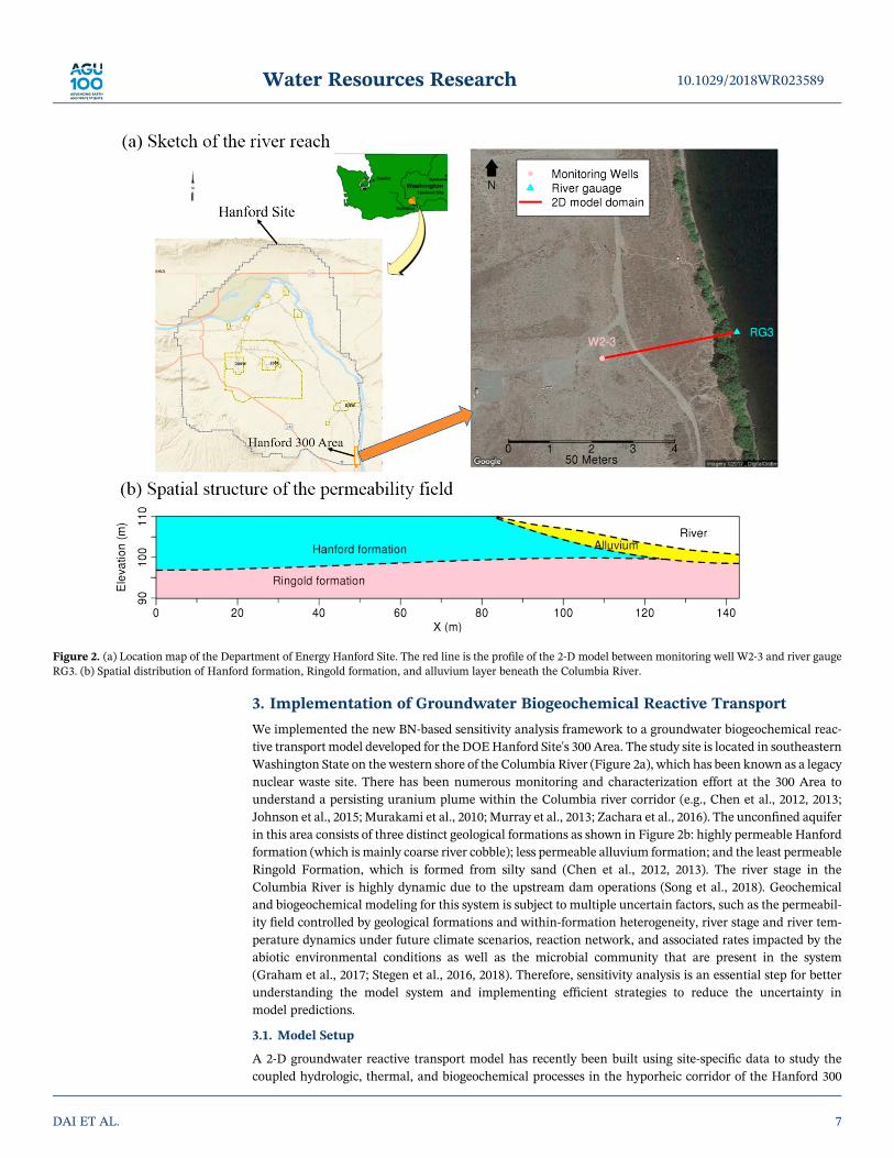
We implemented the new BN‐based sensitivity analysis framework to a groundwater biogeochemical reac-tive transport model developed for the DOEHanford Site's 300 Area. The study site is located in southeasternWashington State on the western shore of the Columbia River (Figure 2a), which has been known as a legacynuclear waste site. There has been numerous monitoring and characterization effort at the 300 Area tounderstand a persisting uranium plume within the Columbia river corridor (e.g., Chen et al., 2012, 2013;Johnson et al., 2015; Murakami et al., 2010; Murray et al., 2013; Zachara et al., 2016). The unconfined aquiferin this area consists of three distinct geological formations as shown in Figure 2b: highly permeable Hanfordformation (which is mainly coarse river cobble); less permeable alluvium formation; and the least permeableRingold Formation, which is formed from silty sand (Chen et al., 2012, 2013). The river stage in theColumbia River is highly dynamic due to the upstream dam operations (Song et al., 2018). Geochemicaland biogeochemical modeling for this system is subject to multiple uncertain factors, such as the permeabil-ity field controlled by geological formations and within‐formation heterogeneity, river stage and river tem-perature dynamics under future climate scenarios, reaction network, and associated rates impacted by theabiotic environmental conditions as well as the microbial community that are present in the system(Graham et al., 2017; Stegen et al., 2016, 2018). Therefore, sensitivity analysis is an essential step for betterunderstanding the model system and implementing efficient strategies to reduce the uncertainty inmodel predictions.

3.1. Model Setup

A 2‐D groundwater reactive transport model has recently been built using site‐specific data to study thecoupled hydrologic, thermal, and biogeochemical processes in the hyporheic corridor of the Hanford 300

Figure 2. (a) Location map of the Department of Energy Hanford Site. The red line is the profile of the 2‐D model between monitoring well W2‐3 and river gaugeRG3. (b) Spatial distribution of Hanford formation, Ringold formation, and alluvium layer beneath the Columbia River.

10.1029/2018WR023589Water Resources Research

DAI ET AL. 7

Area (Song et al., 2018). The numerical model was built using PFLOTRAN, a massively parallel three‐dimensional flow and reactive transport code (Hammond et al., 2014). The model domain is 143.2 m longin the horizontal direction and 20 m deep in the vertical direction. The domain was discretized into approxi-mately 200,000 nonuniform grid cells, with finer grids used in the area closer to the riverbed to better capturethe exchange dynamics and the associated biogeochemical processes at the groundwater‐surface water inter-face. The model domain extended from the Columbia River on the right to an inland well on the left asshown in Figure 2b. A transient hydraulic pressure head boundary and a Dirichlet temperature boundarywere used on both lateral boundaries using the monitoring data obtained from a piezometer in the riverand a groundwater monitoring well at the 300 Area. No‐flow and no‐heat transfer boundary conditions wereused at the top and bottom boundaries. Numerical tracers were placed at the right boundary to track theintrusion of river water in the model domain. The model simulation was conducted for a length of 12 weekscorresponding to one out of six climate scenarios selected from each year of 2010 to 2015 (described insection 3.2). The initial hydraulic head field under each scenario was set to be the average hydraulic headsbetween the inland and river boundaries at the starting time and the temperature field initialized usinginitial temperature at the inland boundary.

The biogeochemical reaction network and the reaction rates in the model were adopted from the work of Liet al. (2017) and H.‐S. Song et al. (2017). The reactions of oxidative respiration and denitrification for the dis-solved organic carbon (CH2O) and the synthesis of biomass (C5H7O2N) were considered as follows:

CH2Oþ O2 ¼ CO2 þH2O

CH2Oþ 2NO−3 ¼ 2NO−

2 þ CO2 þH2O

CH2Oþ 4=3NO−2 þ 4=3Hþ ¼ 2=3N2 þ CO2 þ 5=3H2O

CH2Oþ 1=5NH4þ ¼ 1=5C5H7O2Nþ 3=5H2Oþ 1=5Hþ:

(14)

We used an enzyme‐based cybernetic modeling approach to represent biogeochemical reaction regulated bymicrobial activities (H. Song et al., 2017; X. Song et al., 2018). Temperature‐dependent reaction rate, ri, isdefined using the Arrhenius equation, that is,

ri ¼ rbase;i exp −Ea

R1T−

126þ 273:15

� �� �; i ¼ 1; 2; 3; (15)

where ri is the reaction rate under temperature T (in Kelvin) with subscript i being the generic reactionindex, Ea is the activation energy (0.65 ev in this study), R is the gas constant (8.314 J·mol−1·K−1), andrbase,i is the base rate derived from laboratory batch experiments (under the room temperature of 26 °C).After incorporating microbial regulation term into the Monod kinetics, the base rate, rbase,i, is defined by

rkinbase;i ¼ ereli kidi

Kd;i þ di

aiKa;i þ ai

; i ¼ 1; 2; 3; (16)

where the relative enzyme levels, ereli ¼ rkini =∑3j¼1r

kinj , regulate the rates of oxidative respiration and denitri-

fication reactions (H. Song et al., 2017), ki (mol·L−1·day−1) is the maximum specific uptake rate of organiccarbon (CH2O), ai (mol/L) is the electron acceptor concentration, di (mol/L) is the electron donor concentra-tion, and Ka,i (mol/L) and Kd,i (mol/L) are the half‐saturation constants for electron acceptors and electrondonors, respectively. More details about the reaction network and rates can be found in X. Song et al. (2018).

3.2. Uncertainty Sources

We opt to include six important uncertainty sources: (1) climate scenarios, including time‐varying riverstage, inland well water level, and temperature; (2) the thickness of alluvial layer given a known shape;(3) heterogeneity or homogeneity formulations for the permeability field of Hanford Formation and the allu-vial layer; (4) permeability fields in all of the formations nomatter being homogeneous or heterogeneous; (5)reaction rates for r1, r2, and r3 in equation (15); and (6) whether the heat transport process is modeled toenable temperature‐dependent reaction rates. These uncertainty sources include all scenario, model, andparameter uncertainties: The climate scenario represents the scenario uncertainty, the heterogeneity orhomogeneity of formations and with/without heat transport process represents different physical or

10.1029/2018WR023589Water Resources Research

DAI ET AL. 8

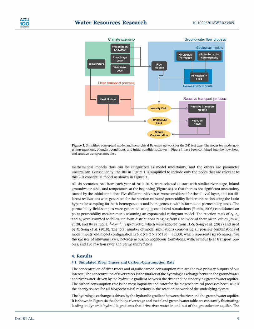
mathematical models thus can be categorized as model uncertainty, and the others are parameteruncertainty. Consequently, the BN in Figure 1 is simplified to include only the nodes that are relevant tothis 2‐D conceptual model as shown in Figure 3.

All six scenarios, one from each year of 2010–2015, were selected to start with similar river stage, inlandgroundwater table, and temperature at the beginning (Figure 4a) so that there is not significant uncertaintycaused by the initial condition. Five different thicknesses were considered for the alluvial layer, and 100 dif-ferent realizations were generated for the reaction rates and permeability fields combination using the Latinhypercube sampling for both heterogeneous and homogeneous within‐formation permeability cases. Thepermeability field samples were generated using geostatistical simulations (Rubin, 2003) conditioned onpoint permeability measurements assuming an exponential variogram model. The reaction rates of r1, r2,and r3 were assumed to follow uniform distributions ranging from 0 to twice of their mean values (28.26,23.28, and 84.78 mol·L−1·day−1, respectively), which were adopted from H.‐S. Song et al. (2017) and usedby X. Song et al. (2018). The total number of model simulations considering all possible combinations ofmodel inputs and model configuration is 6 × 5 × 2 × 2 × 100 = 12,000, which represents six scenarios, fivethicknesses of alluvium layer, heterogeneous/homogeneous formations, with/without heat transport pro-cess, and 100 reaction rates and permeability fields.

4. Results4.1. Simulated River Tracer and Carbon‐Consumption Rate

The concentration of river tracer and organic carbon consumption rate are the two primary outputs of ourinterest. The concentration of river tracer is the marker of the hydrologic exchange between the groundwaterand river water, driven by the hydraulic gradient between the river and the underlying groundwater aquifer.The carbon‐consumption rate is the most important indicator for the biogeochemical processes because it isthe energy source for all biogeochemical reactions in the reaction network of the underlying system.

The hydrologic exchange is driven by the hydraulic gradient between the river and the groundwater aquifer.It is shown in Figure 4a that both the river stage and the inland groundwater table are constantly fluctuating,leading to dynamic hydraulic gradients that drive river water in and out of the groundwater aquifer. The

Figure 3. Simplified conceptual model and hierarchical Bayesian network for the 2‐D test case. The nodes for model gov-erning equations, boundary conditions, and initial conditions shown in Figure 1 have been combined into the flow, heat,and reactive transport modules.

10.1029/2018WR023589Water Resources Research

DAI ET AL. 9

simulated river tracer concentrations in the aquifer are normalized by their concentration in the river (C0),that is, C/C0, and their snapshots at the end of the eighth, tenth, and twelfth weeks of simulation underscenario 1 are shown in Figure 4b for two distinct thicknesses of the alluvial layer. These later time pointsduring the simulation window were selected to minimize the initial condition impacts and to capture

Figure 4. (a) Time series of river stage and water elevation at the model inland boundary at simulation times from 1 January 2010 to 31 December 2015. Thevertical dotted lines demonstrate the six scenario periods under six different years. Two realizations of (b) normalized river tracer concentration and (c) organiccarbon (OC) consumption rate at the three different simulation times under scenario 1 using two distinct thicknesses of the alluvium layer. The homogeneousformation and heat transport process were used for (b) and (c).

10.1029/2018WR023589Water Resources Research

DAI ET AL. 10

longer residence time for biogeochemical reactions. The different geological formation boundaries aremarked using black lines.

The river tracer and carbon‐consumption rate vary in space and time as shown in Figures 4b and 4c, drivenby the hydrologic forcing dynamics demonstrated in Figure 4a. The two examples with distinct alluvial layerthickness shared the same geostatistical realizations of permeability formation, that is, we first selected a rea-lization for the larger spatial domain for each formation and masked the areas that fall outside of the forma-tion for the other case. The river tracer plume first spread from the alluvial layer to the Hanford formationthen started to retreat from the aquifer (Figure 4b), which led to similar spatial pattern for the carbon‐consumption rate (Figure 4c) because the river provides the primary organic carbon source for all the biogeo-chemical reactions with oxygenated conditions on both ends of the domain. Due to the continuous con-sumption of organic carbon along the river water intrusion path, the carbon consumption rates keptreducing accordingly. Consequently, the zone that is biogeochemically active appeared to be smaller thanthe river tracer plume and the biogeochemical reaction rates in the Hanford formation were significantlylower than those in the alluvial layer. The low‐permeability alluvial layer acts as a resistance layer to theriver water intrusion that increases residence time for biogeochemical reactions. Thus, the alluvial thicknessplays a significant role in controlling the spatial extent of river water intrusion. The snapshots associatedwith the case of a thick alluvium layer (Figure 4c) showed significantly more constrained extent of riverwater intrusion and biogeochemical activities compared to the case with thinner alluvial layer. The reactionfront exhibited similarity to the geometry of the thick alluvial layer. There was negligible river tracer and car-bon consumption in the Ringold formation because its low permeability prevents river water infiltration.

4.2. Sensitivity Analysis Results for Carbon‐Consumption Rate

The sensitivity indices corresponding to four primary model input uncertainty sources at the process level,that is, climate scenario, groundwater flow, heat transport, and reactive transport, were calculated for thecarbon‐consumption rates at simulation times of 8, 10, and 12 weeks after the starting point using equa-tion (7). The spatially distributed sensitivity indices are shown in Figure 5, including only the grid cells witha significant average carbon‐consumption rate of 3 × 10−8 mol·m−3·s−1 or more to avoid numerical artifacts.

Both the reactive transport and groundwater flow processes were found to contribute significant uncertain-ties to the carbon‐consumption rate at all three simulation times in most of the biogeochemically activezones, with exceptions in small areas within the river stage fluctuation range where the saturation‐desaturation dynamics controlled the biogeochemical reactions. Thus, the climate scenario contributedthe most uncertainty in these areas, while it contributed the third largest portion of uncertainty to simulatedbiogeochemical reaction rates in general. The reactive transport process appeared to be more important inthe area near the river‐sediment interface where the carbon supply was less limited and flow is slower. Incontrast, the flow process was more dominant in the areas away from river in the Hanford formation wherethe river water intrusion is faster. The heat transport process contributed little to the overall uncertainty,reflected by their small sensitivity indices across the model domain (<0.1). The thermal process was the leastimportant uncertainty source for the carbon‐consumption rate, indicating that the temperature‐dependentreaction rates caused negligible difference in regulating the biogeochemical reactions in this carbon‐limitedsystem, compared to other processes. These sensitivity analysis results were supported by the simulated spa-tial and temporal dynamics of carbon consumption shown in Figure 4 that carbon consumption was drivenby the river water intrusion, which supplied organic carbon for the biogeochemical reactions. Both thegroundwater flow process and driving force scenarios interact to define velocity field dynamics as shownin Figures 1 and 3.

Within the groundwater flow process, its input uncertainty sources can be further attributed to two primarysources: geological formation structures and the permeability field within each formation, as described insection 2.2. Their corresponding sensitivity indices were computed via equation (13) and shown inFigure 5b for simulation times at 8, 10, and 12 weeks. The results illustrated that the geological formationstructure contributed significantly more uncertainty to the flow than the within‐formation permeabilityfield in most of the modeling domain over time. The sensitivity analysis results on flow process componentswere consistent with the observation that the thickness of low‐permeability alluvial layer plays an importantrole for river water intrusion and carbon source infiltration.

10.1029/2018WR023589Water Resources Research

DAI ET AL. 11

5. Conclusions

We developed a new sensitivity analysis framework that integrates the concept of BN‐ and variance‐basedglobal sensitivity analysis. We used a BN to capture the causal relations for a complex numerical modeland represent its various uncertainty sources. The graphical representation of the model system clearlydemonstrates all the causal relationships between the system behaviors (i.e., model outputs) and the variousuncertain components, which greatly facilitates not only the understanding of a complex system but alsocommunicating the scientific understanding to various stakeholders. Combined with a variance‐based glo-bal sensitivity analysis that has been adapted to flexibly grouping variables through the BN, the new frame-work allows the identification of significant uncertainty contributors (a group of variables) in a hierarchicalway beyond a restrictive three‐layer structure. A new set of sensitivity indices on themodel processes or theircomponents was derived following the variance‐based global sensitivity analysis method.

Figure 5. Spatial distribution of sensitivity analysis indices for (a) scenario (SS), groundwater flow (SF), heat transport (SH), and reactive transport processes (SR) atthe simulation times of 8, 10, and 12 weeks. (b) Geological information (SG) and permeability (SP) subprocesses within the groundwater flow process at thesimulation times of 8, 10, 12 weeks. The five thick black lines in the domain represent five distinct alluvium layer thicknesses. OC = organic carbon.

10.1029/2018WR023589Water Resources Research

DAI ET AL. 12

For test and evaluation purposes, the new sensitivity analysis framework was implemented for a real‐worldgroundwater biogeochemical model, which simulated the hydrologic exchange flows and the associatedreactive transport processes at the DOE Hanford Site's 300 Area. A BN was built for the biogeochemicalmodel with six known input uncertainty sources grouped into four primary components at the process level.The sensitivity indices revealed that both the groundwater flow and reactive transport processes contributedsignificantly to the predictive uncertainty in carbon‐consumption rate, followed by the climate scenario thatdefines the driving forces of the system. The heat transport process wasmuch less important compared to theother three processes. Through further decomposition of the uncertainty contributed by groundwater flowprocess to the carbon‐consumption rate, we found that the geological structural information was moreimportant than the within‐formation permeability field in controlling the flow process. The sensitivityindices at the process and subprocess levels all varied in space and time. Therefore, spatial and temporal sen-sitivity indices were essential to understand a dynamic and heterogeneous system.

Although the focus of this research is developing and testing a new sensitivity analyses framework suited forcomplex biogeochemical model, we also demonstrated through the use case that important knowledge andinsights can be gained for improving general biogeochemical reactive transport model through sensitivity. Itis worthmentioning that the BN is built on an acyclic graphic structure. For some natural processes that con-tain cyclic linkages, those nodes should be combined into one aggregate node in BN, such that the sensitivitycontributed from this group could still be quantified although their individual contributions cannot be sepa-rated. The methodology in this research is also mathematically rigorous and generally applicable to a widerange of multiprocess earth system problems to reduce the predictive uncertainty by identifying the mostimportant uncertainty contributors.

ReferencesAguilera, P. A., Fernandez, A., Fernandez, R., Rumi, R., & Salmeron, A. (2011). Bayesian networks in environmental modelling.

Environmental Modelling and Software, 26(12), 1376–1388. https://doi.org/10.1016/j.envsoft.2011.06.004Aguilera, P. A., Fernandez, A., Ropero, R. F., & Molina, L. (2013). Groundwater quality assessment using data clustering based on hybrid

Bayesian networks. Stochastic Environmental Research and Risk Assessment, 27(2), 435–447. https://doi.org/10.1007/s00477‐012‐0676‐8Basso, S., Schirmer, M., & Botter, G. (2016). A physically based analytical model of flood frequency curves. Geophysical Research Letters, 43,

9070–9076. https://doi.org/10.1002/2016GL069915Chen, X., Hammond, G. E., Murray, C. J., Rockhold, M. L., Vermeul, V. R., & Zachara, J. M. (2013). Application of ensemble‐based data

assimilation techniques for aquifer characterization using tracer data at Hanford 300 area. Water Resources Research, 49, 7064–7076.https://doi.org/10.1002/2012WR013285

Chen, X., Murakami, H., Hahn, M. S., Hammond, G. E., Rockhold, M. L., Zachara, J. M., & Rubin, Y. (2012). Three dimensional Bayesiangeostatistical aquifer characterization at the Hanford 300 Area using tracer test data.Water Resources Research, 48, W06501. https://doi.org/10.1029/2011WR010675

Chu‐Agor, M. L., Muñoz‐Carpena, R., Kiker, G., Emanuelsson, A., & Linkov, I. (2011). Exploring sea level rise vulnerability of coastalhabitats through global sensitivity and uncertainty analysis. Environmental Modelling and Software, 26(5), 593–604. https://doi.org/10.1016/j.envsoft.2010.12.003

Clark, M. P., Nijssen, B., Lundquist, J. D., Kavetski, D., Rupp, D. E., Woods, R. A., et al. (2015). A unified approach for process‐basedhydrologic modeling: 2. Model implementation and case studies. Water Resources Research, 51, 2515–2542. https://doi.org/10.1002/2015WR017200

Clark, M. P., Schaefli, B., Schymanski, S. J., Samaniego, L., Luce, C. H., Jackson, B. M., et al. (2016). Improving the theoretical underpin-nings of process‐based hydrologic models. Water Resources Research, 52, 2350–2365. https://doi.org/10.1002/2015WR017910

Dai, H., Chen, X., Ye, M., Song, X., & Zachara, J. (2017). A geostatistics informed hierarchical sensitivity analysis method for complexgroundwater flow and transport modeling. Water Resources Research, 53, 4327–4343. https://doi.org/10.1002/2016WR019756

Dai, H., & Ye, M. (2015). Variance‐based global sensitivity analysis for multiple scenarios and models with implementation using sparsegrid collocation. Journal of Hydrology, 528, 286–300. https://doi.org/10.1016/j.jhydrol.2015.06034

Dai, H., Ye, M., Hu, B. X., Niedoroda, A. W., Zhang, X., Chen, X., et al. (2018). Hierarchical sensitivity analysis for simulating barrier islandgeomorphologic responses to future storms and sea‐level rise. Theoretical and Applied Climatology. https://doi.org/10.1007/s00704‐018‐2700‐5

Dai, H., Ye, M., Walker, A. P., & Chen, X. (2017). A new process sensitivity index to identify important system processes under processmodel and parametric uncertainty. Water Resources Research, 53, 3476–3490. https://doi.org/10.1002/2016WR019715

Dai, Z., & Samper, J. (2004). Inverse problem of multicomponent reactive chemical transport in porous media: Formulation and applica-tions. Water Resources Research, 40, W07407. https://doi.org/10.1029/2004WR003248

Darwiche, A. (2009). Modeling and reasoning with Bayesian networks. New York: Cambridge University Press. https://doi.org/10.1017/CBO9780511811357

Graham, E. B., Tfaily, M. M., Crump, A. R., Goldman, A. E., Bramer, L. M., Arntzen, E., et al. (2017). Carbon inputs from riparian vege-tation limit oxidation of physically bound organic carbon via biochemical and thermodynamic processes. Journal of GeophysicalResearch: Biogeosciences, 122, 3188–3205. https://doi.org/10.1002/2017JG003967

Grayson, R. B., & Bloschl, G. (2000). Spatial patterns in catchment hydrology: Observations and modeling. Cambridge, UK: CambridgeUniversity Press.

Hammond, G. E., Lichtner, P. C., & Mills, R. T. (2014). Evaluating the performance of parallel subsurface simulators: An illustrativeexample with PFLOTRAN. Water Resources Research, 50, 208–228. https://doi.org/10.1002/2012WR013483

10.1029/2018WR023589Water Resources Research

DAI ET AL. 13

AcknowledgmentsThis research was supported by the U.S.Department of Energy (DOE), Office ofBiological and Environmental Research(BER), as part of BER's SubsurfaceBiogeochemical Research Program(SBR). A portion of methodologyimprovement was supported by theLaboratory Directed Research andDevelopment Program at PacificNorthwest National Laboratory, amultiprogram national laboratoryoperated by Battelle for DOE undercontract DE‐AC05‐76RL01830. The firstauthor was supported in part by theNational Natural Science Foundation ofChina (NSFC) project 41807182. Thethird author was supported in part byDOE grants DE‐SC0019438 and DE‐SC0008272 and NSF‐EAR grant1552329. This research used resourcesof the National Energy ResearchScientific Computing Center, a DOEOffice of Science‐supported UserFacility under contract DE‐AC02‐05CH11231. The data used in the ana-lyses can be downloaded online(https://sbrsfa.velo.pnnl.gov:443/data-sets/?UUID=79b70800‐5f91‐4da1‐a1b3‐24c0058684bc).

Heckerman, D. (1997). Bayesian networks for data mining. Data Mining and Knowledge Discovery, 1(1), 79–119. https://doi.org/10.1023/A:1009730122752

Herman, J. D., Reed, P. M., & Wagener, T. (2013). Time‐varying sensitivity analysis clarifies the effects of watershed model formulation onmodel behavior. Water Resources Research, 49, 1400–1414. https://doi.org/10.1002/wrcr.20124

Johnson, T., Versteeg, R., Thomle, J., Hammond, G., Chen, X., & Zachara, J. (2015). Four‐dimensional electrical conductivity monitoring ofstage‐driven river water intrusion: Accounting for water table effects using a transient mesh boundary and conditional inversion con-straints. Water Resources Research, 51, 6177–6196. https://doi.org/10.1002/2014WR016129

Kjaerulff, U. B., & Madsen, A. L. (2008). Bayesian networks and influence diagrams: A guide to construction and analysis. New York, NY,USA: Springer Science + Business Media. https://doi.org/10.1007/978‐0‐387‐74101‐7

Li, M., Qian, W. J., Gao, Y., Shi, L., & Liu, C. (2017). Functional enzyme‐based approach for linking microbial community functions withbiogeochemical process kinetics. Environmental Science & Technology, 51(20), 11,848–11,857. https://doi.org/10.1021/acs.est.7b03158

Murakami, H., Chen, X., Hahn, M. S., Liu, Y., Rockhold, M. L., Vermeul, V. R., et al. (2010). Bayesian approach for three‐dimensionalaquifer characterization at the Hanford 300 Area.Hydrology and Earth System Sciences, 14(10), 1989–2001. https://doi.org/10.5194/hess‐14‐1989‐2010

Murray, C. J., Zachara, J. M., McKinley, J. P., Ward, A., Bott, Y. J., Draper, K., &Moore, D. (2013). Establishing a geochemical heterogeneitymodel for a contaminated vadose zone–Aquifer system. Journal of contaminant hydrology, 153, 122–140. https://doi.org/10.1016/j.jconhyd.2012.02.003

Neuman, S. P. (2003). Maximum likelihood Bayesian averaging of alternative conceptual‐mathematical models. Stochastic EnvironmentalResearch and Risk Assessment, 17(5), 291–305. https://doi.org/10.1007/s00477‐003‐0151‐7

Pearl, J. (2014). Probabilistic reasoning in intelligent systems: Networks of plausible inference (2nd ed.). San Francisco, CA: MorganKaufmann Publishers, INC.

Razavi, S., & Gupta, H. V. (2015). What do we mean by sensitivity analysis? The need for comprehensive characterization of “global”sensitivity in earth and environmental systems models. Water Resources Research, 51, 3070–3092. https://doi.org/10.1002/2014WR016527

Refsgaard, J. C., Christensen, S., Sonnenborg, T. O., Seifert, D., Hojberg, A. L., & Troldborg, L. (2012). Review of strategies for handlinggeological uncertainty in groundwater flow and transport modeling. Advances in Water Resources, 36, 36–50. https://doi.org/10.1016/j.advwatres.2011.04.006

Rubin, Y. (2003). Applied stochastic hydrogeology. Oxford University Press.Saltelli, A., & Sobol', I. M. (1995). About the use of rank transformation in sensitivity analysis of model output. Reliability Engineering and

System Safety, 50(3), 225–239. https://doi.org/10.1016/0951‐8320(95)00099‐2Saltelli, A. (2000). What is sensitivity analysis? In A. Saltelli, K. Chan, & M. Scott (Eds.), Sensitivity analysis (pp. 3–14). Chichester: Wiley.Saltelli, A., Annoni, P., Azzini, I., Campolongo, F., Ratto, M., & Tarantola, S. (2010). Variance based sensitivity analysis of model output.

Design and estimator for the total sensitivity index. Computer Physics Communications, 181(2), 259–270. https://doi.org/10.1016/j.cpc.2009.09.018

Saltelli, A., Tarantola, S., & Chan, K. P.‐S. (1998). Presenting results from model based studies to decision makers: Can sensitivity analysisbe a defogging agent? Risk Analysis, 18(6), 799–803. https://doi.org/10.1111/j.1539‐6924.1998.tb01122.x

Saltelli, A., Tarantola, S., & Chan, K. P.‐S. (1999). A quantitative model independent method for global sensitivity analysis of model output.Technometrics, 41(1), 39–56. https://doi.org/10.1080/00401706.1999.10485594

Sivakumar, B. (2004). Dominant processes concept in hydrology: Moving forward. Hydrological Processes, 18(12), 2349–2353. https://doi.org/10.1002/hyp.5606

Sivakumar, B. (2008). Dominant processes concept, model simplification and classification framework in catchment hydrology. StochasticEnvironmental Research and Risk Assessment, 22(6), 737–748. https://doi.org/10.1007/s00477‐007‐0183‐5

Sobol', I. M. (1993). Sensitivity analysis for nonlinear mathematical models. Mathematical Modeling and Computational Experiment, 1(4),407–414.

Song, H.‐S., Thomas, D., Stegen, J., Li, M., Liu, C., Song, X., et al. (2017). Regulation‐structured dynamic metabolic model provides apotential mechanism for delayed enzyme response in denitrification process. Frontiers in Microbiology, 8, 1866. https://doi.org/10.3389/fmicb.2017.01866

Song, X., Chen, X., Stegen, J., Hammond, G., Dai, H., Graham, E., & Zachara, J. M. (2018). Drought conditions maximize the impacts ofhigh‐frequency flow variations on thermal regimes and biogeochemical function in the hyporheic zone. Water Resources Research, 54,7361–7382. https://doi.org/10.1029/2018WR022586

Song, X., Zhang, J., Zhan, C., Xuan, Y., Ye, M., & Xu, C. (2015). Global sensitivity analysis in hydrological modeling: Review of con-cepts, methods, theoretical framework, and applications. Journal of Hydrology, 523, 739–757. https://doi.org/10.1016/j.jhydrol.2015.02.013

Stegen, J. C., Fredrickson, J. K., Wilkins, M. J., Konopka, A. E., Nelson, W. C., Arntzen, E. V., & Tfaily, M. (2016). Groundwater–surfacewater mixing shifts ecological assembly processes and stimulates organic carbon turnover. Nature Communications, 7(1), 11237. https://doi.org/10.1038/ncomms11237

Stegen, J. C., Johnson, T., Fredrickson, J. K., Wilkins, M. J., Konopka, A. E., Nelson, W. C., & Zachara, J. (2018). Influences of organiccarbon speciation on hyporheic corridor biogeochemistry and microbial ecology. Nature Communications, 9(1), 585. https://doi.org/10.1038/s41467‐018‐02922‐9

Tartakovsky, D. M. (2013). Assessment and management of risk in subsurface hydrology: A review and perspective. Advances in WaterResources, 51, 247–260. https://doi.org/10.1016/j.advwatres.2012.04.007

van Griensven, A., Meixner, T., Grunwald, S., Bishop, T., Diluzio, M., & Srinivasan, R. (2006). A global sensitivity analysis tool for theparameters of multi‐variable catchment models. Journal of Hydrology, 324(1‐4), 10–23. https://doi.org/10.1016/j.jhydrol.2005.09.008

Velikova, M., Scheltinga, J. T. V., Lucas, P. J. F., & Spaanderman, M. (2014). Exploiting causal functional relationships in Bayesian networkmodeling for personalised healthcare. International Journal of Approximate Reasoning, 55(1), 59–73. https://doi.org/10.1016/j.ijar.2013.03.016

Wainwright, H. M., Finsterle, S., Jung, Y., Zhou, Q., & Birkholzer, J. T. (2014). Making sense of global sensitivity analysis. ComputationalGeosciences, 65, 84–94. https://doi.org/10.1016/j.cageo.2013.06.006

Ye, M., Neuman, S. P., & Meyer, P. D. (2004). Maximum likelihood Bayesian averaging of spatial variability models in unsaturated frac-tured tuff. Water Resources Research, 40, W05113. https://doi.org/10.1029/2003WR002557

Ye, M., Neuman, S. P., Meyer, P. D., & Pohlmann, K. F. (2005). Sensitivity analysis and assessment of prior model probabilities in MLBMAwith application to unsaturated fractured tuff. Water Resources Research, 41, W12429. https://doi.org/10.1029/2005WR004260

10.1029/2018WR023589Water Resources Research

DAI ET AL. 14

Ye, M., Pohlmann, K. F., & Chapman, J. B. (2008). Expert elicitation of recharge model probabilities for the Death Valley regional flowsystem. Journal of Hydrology, 354(1‐4), 102–115. https://doi.org/10.1016/j.jhydrol.2008.03.001

Zachara, J., Brantley, S., Chorover, J., Ewing, R., Kerisit, S., Liu, C., et al. (2016). Internal domains of natural porousmedia revealed: Criticallocations for transport, storage, and chemical reaction. Environmental Science & Technology, 50(6), 2811–2829. https://doi.org/10.1021/acs.est.5b05015

10.1029/2018WR023589Water Resources Research

DAI ET AL. 15