Using Battleground States as a Natural Experiment to Test ...Using Battleground States as a Natural...

Using Battleground States as a Natural Experiment to Test Theories of Voting*

Alan S. Gerber Yale University

Department of Political Science Institution for Social and Policy Studies

77 Prospect Street, PO Box 208209 New Haven, CT 06520-8209

[email protected]

Gregory A. Huber Yale University

Department of Political Science Institution for Social and Policy Studies

77 Prospect Street, PO Box 208209 New Haven, CT 06520-8209

[email protected]

Conor M. Dowling Yale University

Institution for Social and Policy Studies 77 Prospect Street, PO Box 208209

New Haven, CT 06520-8209 [email protected]

David Doherty Yale University

Institution for Social and Policy Studies 77 Prospect Street, PO Box 208209

New Haven, CT 06520-8209 [email protected]

Nicole Schwartzberg

Yale University [email protected]

* A previous version of this paper was presented at the annual meeting of the American Political Science Association, Toronto, Canada, September 3-6, 2009. We thank Jamie Carson for comments on that earlier draft.

ABSTRACT: We use variation produced by the Electoral College—the creation of battleground and non

battleground states—to examine explanations for why people vote. We employ a longer time series

(1980-2008) than previous research to gauge the effect of battleground status on state-level turnout. Our

model includes (1) midterm elections, allowing us to directly compare the effect of battleground status

with the broader increase in turnout associated with presidential elections, and (2) state fixed effects,

which capture persistent state-level factors related to turnout. We find that the turnout boost from a

presidential election is eight times the effect of being a battleground state. This suggests turnout is

primarily linked to factors affecting the entire electorate, such as the social importance of presidential

elections, rather than factors that influence just a portion of the country, such as intensive campaigning

and mobilization efforts or a greater chance of casting a decisive vote.

Understanding the level of and variation in electoral participation rates has absorbed the attention

of scholars for decades. There is no consensus on which set of factors accounts best for the decision to

vote, but researchers have offered a number of explanations. The economic theory of voting depicts

voters weighing the costs of voting against the potential benefits of casting a decisive vote (Downs 1957).

Other theoretical and empirical studies emphasize a sense of civic duty (Riker and Ordeshook 1968),

social pressure (Gerber, Green, and Larimer 2008), mobilization efforts (Gerber and Green 2000;

Rosenstone and Hansen 1993), and cost-benefit calculations pertaining to the convenience of voting (e.g.,

Brady and McNulty 2004; Dyck and Gimpel 2005) as affecting whether a person votes.

In this paper, we exploit variation across states produced by the Electoral College system used in

U.S. Presidential elections—the creation of “battleground” and “non battleground” states—to assess some

of these explanations. Relative to their non battleground counterparts, battleground states receive an

immense amount of attention from the parties because they are believed to be pivotal to the outcome of

the election.1 The contrast between turnout in battleground and non battleground states gives us a measure

of how much both the “pivotalness” of one’s vote and intensive campaigning and mobilization efforts in

battleground states affect the chances an individual votes. Because our model includes observations from

both presidential and midterm election years, we are also able to compare the size of this “battleground”

effect to the effect a presidential election has on turnout across all states (whether a battleground or not),

which we argue encapsulates the effects of those features of presidential elections which affect all

citizens, such as the national focus on electing the most important political officer in the nation.

In addition, this paper makes three more technical contributions to the literature on the effects of

battleground status on turnout. First, we examine the effect of battleground status on state-level turnout 1 In 2008, for example, John McCain ($333 million) and Barack Obama ($730 million) combined to spend more than one billion dollars for the first time in history (Source: OpenSecrets.org), but “more than 98% of all campaign events and more than 98% of all campaign spending took place in only 15 states,” with the majority of these events and this spending taking place in only four states: Florida, Ohio, Pennsylvania, and Virginia (Source: FairVote.org). For theories and evidence on how the Electoral College influences campaign resource allocation strategies see Brams and Davis (1974); Colantoni, Levesque, and Ordeshook (1975); Bartels (1985); Cox and Munger (1989); James and Lawson (1999); Shaw (1999b, 2006); Reeves, Chen, and Nagano (2004); Strömberg (2008); Goux (2009); Shachar (2009).

from 1980-2008 using statistical models that include both presidential and midterm election years. This

allows us to estimate both the effect of being in a battleground state in a presidential election and the

effect of the presidential election (compared to the midterm election) itself. Second, the length of our time

series allows us to include state-level fixed effects in our model, thereby allowing us to control for any

(measured or unmeasured) fixed, state-level characteristics that may be correlated with battleground

status. Third, we also analyze the effect of changes in battleground status on change in turnout, which

provides a way to separate the effect of status as a battleground state in the current election from any

carryover effect from being a battleground state in the previous election.

Our main finding is that the effect of presidential elections on turnout dwarfs the effect of being

in a pivotal (battleground) state (the presidential election produces eight times the effect of battleground

status). Moreover, for all the attention devoted to battleground states—from 1988-2008, on average, they

received more than 80% of presidential campaign visits and advertising dollars (Shaw 1999a, 2006;

Huang and Shaw forthcoming), turnout is only on average about one to two percentage points higher than

in non battleground states. The large increase in turnout in presidential elections in all states, battleground

and “spectator” states alike, suggests turnout levels are linked to factors that affect the entire electorate,

such as perceptions about the importance of the presidency or the prominence of the national election as a

topic of conversation, rather than factors that influence just a portion of the country, such as targeted

campaigning and mobilization efforts or a greater chance of casting a decisive ballot.

The remainder of this paper proceeds as follows. In the next section we discuss previous research

on the effect of battleground status on voter turnout. We then present the model we use to test for the

effects of battleground status on turnout, and discuss how it is an improvement over previous research.

Next, we present our data and results, which show that the effect of status as a battleground state on

turnout using an expanded set of elections is somewhat more modest than most recent research suggests,

and is clearly much smaller than the common increase associated with the nationwide presidential

election. We conclude with a discussion of the implications our findings have for understanding

explanations for why people vote.

1. Previous Research: Battleground Status and Turnout

A handful of recent studies have examined the effect of living in a battleground state on voter

turnout. These studies employ different data, sometimes focusing on one year, other times on multiple

years, and use different methodological approaches. While nearly all studies find the effect of

battleground status to be less than about four percent, the specific estimates have been mixed. The results

of these seven studies, including years studied and measures of battleground status and turnout, are

summarized in Table 1.

<Insert Table 1 about here>

Three single-year studies find that battleground states have substantially higher turnout than non

battleground states. McDonald (2008) observes that in 2008 turnout in the ten battleground states—

classified as states that were visited by candidates from both campaigns in the last two weeks of the

election—was four percentage points higher (65.9 versus 61.9%) than the remaining forty states.2

However, McDonald’s bivariate comparison does not control for any other factors that might also be

related to turnout at the state level, such as whether a senatorial election was also being held in the state or

baseline turnout levels in the state (e.g., turnout levels irrespective of the presidential race or battleground

status). Bergan et al. (2005, see Table 4) examine the 2004 election and do control for these factors.

Controlling for lagged battleground status and the average turnout in the state in the two previous

midterm elections, they find that there was about a four or five percentage point turnout gap between

battleground (measured using CNN state rankings) and non battleground states in 2004.3 Analyzing the

2000 election, Hill and McKee (2005, 715) find that the effect of battleground status (using Shaw’s

[1999b, 2006] classification system4) on turnout is slightly less than two percentage points. Although the

2 These ten battleground states are: Colorado, Florida, Indiana, Iowa, Missouri, Nevada, North Carolina, Ohio, Pennsylvania, and Virginia. 3 Bergan et al. (2005, Table 5) estimate another model predicting change in turnout that includes a lag for previous battleground status, which accounts for a change in battleground status from one election to the next. The coefficient for current battleground status in this regression is +3.67 (p<.001). 4 Shaw (1999b, 2006) identifies battleground states based upon information given to him by campaign consultants involved in planning the Electoral College strategies of the presidential candidates. He asked campaign strategists from each party to label every state as either (1) safe for one party (e.g., “base

size of the battleground effect varies across these single-year studies, they tend to suggest that turnout is

considerably higher in battleground states.

Findings from multi-year studies are also somewhat mixed. In a study using the predicted

closeness of the presidential race in the state—estimated by Campbell’s (1992) model for forecasting

election results—to measure a state’s relative competitiveness, Shachar and Nalebuff (1999, see Table 6)

estimate a structural model of participation and conclude “a 55:45 race should have a 1-percent higher

participation rate than a 60:40 race” (532).5 In their analyses of presidential elections from 1992 to 2000,

Holbrook and McClurg (2005) and Wolak (2006) report no difference in turnout rates between those

states that are deemed to be battlegrounds and those that are not. Holbrook and McClurg use state-level

turnout and campaign (presidential visits and media purchases and party transfers to the states) data and

find that the parties focus on, and succeed at, mobilizing “core supporters” across states, but “find no

clear evidence that the importance of campaigns for mobilization is dependent on competition in the

states” (701, see Table 1). Examining the same sets of elections, but with American National Election

Study (ANES) survey data, Wolak (see Table 3) also finds no effect of campaign battleground strategy

(presidential advertising and campaign visits) on turnout intentions. Thus, two analyses of the same

presidential elections (1992, 1996, and 2000) using different sets of data reach the same conclusion that

living in a battleground state has no effect on turnout. In addition to considering only three elections,

neither of these studies includes midterm election years or state fixed effects.

In a recent article, Lipsitz (2009) argues that “we should expect to see greater E[lectoral]

C[ollege] campaign strategy effects when elections are close than when there is a clear frontrunner” Republican”), (2) leaning toward one party (e.g., “lean Republican”), or (3) as a “battleground.” This creates five possible categories for each state. Hill and McKee (2005) consider those states that both parties assert are “battlegrounds” to be battleground states in their analysis, which they argue is appropriate given the fact that there was strong agreement between the parties in 2000. Other studies have used Shaw’s Electoral College strategy data to create a five-point measure of state competitiveness ranging from 0 (if both campaigns said a state was a safe state) to 4 (if both campaigns said a state was a battleground state) by summing Shaw’s scores for each party (where “base” equals 0, “lean” equals 1, and “battleground” equals 2) (see Gimpel, Kaufmann, and Pearson-Merkowitz 2007; Lipsitz 2009). 5 For a theoretical account, see Shachar (2009), who concludes that there is no direct effect of predicted closeness on turnout. Rather, his findings suggest that the effect of predicted closeness on turnout is only an indirect one through “marketing activities” (i.e., political advertising and other campaign efforts).

(192). This leads her to hypothesize that, of the five presidential elections in her data set (1988-2004), the

“effects [of battleground status] should be largest in 1988, 2000 and 2004 because of the competitiveness

of those [national] elections” (193). According to this account, of the three elections analyzed by

Holbrook and McClurg (2005) and Wolak (2006), only one (2000) is expected to exhibit substantial

battleground state effects, which explains the null findings reported in those studies. Lipsitz finds a three

percentage point turnout gap between battleground (defined by Shaw’s classification system, see footnote

4) and spectator states in 2000 and a six percentage point gap in 2004. Although Lipsitz’s important study

controls for average turnout in the preceding two midterm elections, her model does not include midterm

elections (as cases) and also does not include state fixed effects. In addition, the ex-post classification of

races as “close” may not capture the anticipated closeness of the election. Further, if winning is the goal,

concentrating campaign resources on a set of battleground states makes strategic sense even when the

final outcome is less competitive.

1.1 Extending Previous Work on the Effects of Battleground Status on Turnout

We seek to build on previous studies in three ways. First, we include midterm elections as part of

our data set so that we can make a direct comparison between the effect of being a battleground state in a

presidential election and the effect of the presidential election itself. The relative magnitude of these

effects can offer insight into what voters are thinking when they decide whether to vote. Second, we

employ a time series (1980 to 2008) that is long enough to provide sufficient degrees of freedom to

include state fixed effects. The inclusion of state-level fixed effects ensures that the coefficient on our

indicator of battleground status can be interpreted as the effect of being a battleground state on turnout,

rather than any other state-level factors that may be correlated with both battleground status and turnout.

Third, previous work attributes the effect of being a battleground state on turnout to being a

battleground state in that election, which may produce misleading estimates because not many states

move in and out of the “battlefield” (a problem magnified by a lack of state fixed effects). Thus, it could

be the case that a longstanding history as a battleground state is what a “battleground” coefficient is

estimating. If battleground status matters more when a state first enters the battlefield (or does so after a

hiatus), then the effect of battleground status observed in previous work may overestimate the effect of

continued battleground status and underestimate the effect of becoming a battleground. Indeed, there is

some suggestive evidence that this could be the case. As McDonald notes for the 2008 election,

New entrants to the Electoral College battleground in 2008 experienced the largest turnout increases from 2004. Thus Indiana’s turnout rate rose 4.5 percentage points, from 54.8% to 59.3%; North Carolina improved 8.0 percentage points, from 57.8% to 65.8%; and Virginia increased 6.8 percentage points, from 60.6% to 67.4%. States that left the battlefield, such as Maine, Minnesota, Oregon, Washington and Wisconsin, experienced turnout declines or failed to keep pace with the national increase. Other states that remained in play essentially had the same levels of turnout (2008, 2).

Thus, we believe a potentially more informative test of whether battleground status at time t affects

turnout at time t is to examine changes in battleground status from time t-1.

2. Modeling the Effect of Battleground Status on State-level Turnout

To concretely illustrate the advantages of an approach employing (1) midterm election years, (2)

state fixed effects, and (3) changes in battleground status, we outline our modeling strategy by first

detailing how it deviates from previous work. Consider first a model of the single-year case in which

state-level turnout (TOi, the i subscript denotes states) is the dependent variable, and the independent

variable is whether a state is considered a battleground (BGi = 1) or not (BGi = 0). In this instance, we

estimate the effect of BG on TO using the following model:

(1) TOi = B0 + B1BGi + Ui,

where Ui represents unobserved error in the model. In (1), the effect of BG is biased if the disturbance

term, Ui, contains omitted determinants of TOi that are correlated with battleground status. Studies of the

effect of battleground status on turnout typically account for this concern by including some measure of

the baseline turnout rate (BTi) of a state and a vector (Zi) of other control variables, such as whether a

senatorial or gubernatorial election is also being held in the state during that year, because these factors

are also likely to affect TO in the presidential election. With these controls, we can rewrite (1) as:

(2) TOi = B0 + B1BGi + B2BTi + γZi + Ui.

However, the inclusion of BT and Z (e.g., senatorial and gubernatorial election indicators) does not solve

the problem of being able to identify the direct effect of BG on TO because what determines BG may be

correlated with omitted variables across states (e.g., the presence of particularly close House or state level

elections, or more developed state parties).

This is the case even in a panel design that only examines presidential election years:

(3) TOi,t = B0 + B1BGi,t + B2BTi,t + γZi,t + τTt + Ui,t,

where the new subscript t denotes time, and T is a vector of year-specific intercepts. In this panel design,

there is still uncertainty surrounding the causal relationship between BG and TO if there are omitted

factors (in U) that are correlated with both BG and TO. Moreover, even if model (3) were perfectly

specified (i.e., U has a mean of 0), it does not allow us to estimate the effect of having a presidential

election relative to not having one because midterm elections are not included.

In order to isolate the effects of the presidential election and being a battleground state in a

presidential election, we include in our model both midterm and presidential elections. Thus, we rewrite

(3) as:

(4) TOi,t = B0 + B1BGi,t + B2Pt + γZi,t + τTt + ψSi + Ui,t,

where the new terms are P and S. P is a dichotomous indicator for whether the current election is a

presidential or midterm election that does not vary across states. S is a vector of state indicators, used to

estimate state fixed effects. These fixed effects account for any time-invariant characteristics that affect

state-level turnout. We note that even with the inclusion of the state fixed effects, this model does not

permit us to estimate the effect of changes in battleground status on turnout. In order to do so, we employ

two approaches: (1) we introduce one and two election lags for battleground status and (2) we regress

change in turnout on changes in battleground status. (We describe each of these approaches in greater

detail below.)

3. Data and Results

We use the variation in the choice environment across battleground and non battleground states to

test theories of voting based on an assumption that any turnout effects of battleground status stem from

the fact that people in these states are (quasi-randomly) assigned to receive more intensive campaign

efforts and have a greater likelihood that their votes are decisive for the election outcome. In contrast, any

common effect of a presidential election on turnout presumably is a product of factors that affect the

entire electorate. For this study to approximate a “natural experiment,” it must be the case that

battleground states are not created by some underlying process or mechanism that is related to state-level

turnout. We offer a number of observations in defense of this assumption here.

We begin by noting that, given that we include state fixed effects in our model (see above), any

underlying source of variation that affects both status as a battleground state and voter turnout must

change over time (i.e., it cannot be a stable characteristic). One possible source of change is that new

migrants may cause a state to become more competitive because the migrants’ ideological dispositions

may mitigate the dominant ideology present in the state. While there are certainly fluctuations in state

population size, they do not appear to be linked to changes in state competitiveness. For instance, in

presidential elections from 1980-2008, the state-level change in the voting age population (VAP) is

correlated with the two-party margin of victory in the state at r = -.08 and changes in the two-party

margin of victory in the state at r = -.03. Thus, there does not appear to be any strong evidence that

changes in the adult population in a state from one presidential election to the next make the state

substantially more competitive. Moreover, changes in a state’s VAP are only weakly correlated with

changes in turnout in the state from one presidential election to the next at r = .04.

Another possibility is that presidential candidates change the competitive environment in their

home states. From 1980 to 2008 five presidential home states move into (two states) or out of (three

states) battleground status based on our measure of state pivotalness (described below).6 In addition, from

1980 to 2008 presidential home states are weakly and positively correlated with a state’s two-party

margin of victory (r = .06), suggesting that on average president’s make their home state’s less

competitive. However, changes in the two-party margin of victory are almost completely uncorrelated

with the home state of presidential candidates (r = .01), suggesting presidential candidates do not

substantially change the competitive environments of their home states. We find similarly weak

6 CA (1984 - Reagan) and TX (1988 - Bush) become pivotal states, while CA (1980 - Reagan), TX (1992 - Bush), and AZ (2008 - McCain) are no longer pivotal.

correlations between an indicator for presidential candidate home state and both turnout (r = -.07, 1980-

2008) and changes in turnout (r = -.002, 1984-2008).7

3.1 Data

Our time series extends from 1980-2008 and includes 750 observations (50 states x 15 elections

[7 midterm, 8 presidential]).8 We specify state-level voter turnout as percent turnout (0-100) among the

voting eligible population (VEP). The VEP data were collected and made available by Professor Michael

P. McDonald.9 For battleground status we cannot rely solely on Shaw’s classification of battleground

states, which is based on his reports from the campaigns, because our time series includes two elections

(1980 and 1984) that Shaw does not classify. Instead, we create a measure of state “battlegroundness” (or,

more accurately, whether the state was pivotal to the election outcome) based on actual election

outcomes, and use Shaw’s categorization as a robustness check for the years it is available (1988-2008,

see Shaw 1999b, 2006 and Huang and Shaw forthcoming).

We measure the pivotalness of the state to the overall electoral outcome based on the actual

election outcome observed in the state. Specifically, for each presidential election year, we arrayed the

states by the Democratic share of the two-party vote and then cumulatively summed the Electoral College

votes by state in this order. We then subtracted that number from 270 (the number of Electoral College

votes needed in order to be declared the victor) and took the absolute value of that figure. This gives us an

indicator of how likely it was that the state was pivotal in determining the outcome of the election. We

7 If we omit candidate home states from the analyses presented below, the substantive conclusions we draw do not change. These results are available upon request. 8 In 1982, Louisiana did not hold congressional elections in November because all of the races were settled earlier in the election season during Louisiana’s open primary. Therefore, there is no recorded turnout for Louisiana in the 1982 general election and we lose this observation from our data set, making our total number of observations 749. 9 The data can be downloaded from: http://elections.gmu.edu/Turnout.html (McDonald 2009). The data only extend back to 1980. Therefore, when we include lagged turnout in some of the model specifications presented below (Appendix Table A3), we use the voting age population (VAP) as our denominator for calculating state-level voter turnout because this allows us to calculate turnout rates for years prior to 1980.

classified any state that was within 100 electoral votes of 270 as a pivotal state (i.e., battleground).10 See

Appendix Table A1 for a list of pivotal states from 1972-2008 based on this measure. Most people are

aware of how pivotal their vote is to the election outcome (see Blais 2000, chapter 3).11 We confirm that

our measure also correlates with the distribution of campaign activity in presidential elections empirically.

Table 2 displays presidential advertising12 and campaign visit data from 1988-2008 (see Shaw 1999a,

2006; Huang and Shaw forthcoming) in battleground (BG) and non battleground (NBG) states based on

both our measure (left hand side of the table) and Shaw’s (right hand side of the table). The table

highlights the discrepancy between BG and NBG states in both the number of visits and the amount of

money spent on advertising: battleground states always receive substantially more of both. Thus, our

indicator appears to measure aspects of the presidential campaign linked to battleground states.


As a further validity and reliability check of our pivotal state measure, we compare our measure

to Shaw’s classification system (described in footnote 4 and used in previous work [Gimpel, Kaufmann,

and Pearson-Merkowitz 2007; Hill and McKee 2005; Lipsitz 2009]). Specifically, if either party reported

to Shaw that a given state was a “battleground” we give it a score of one; if neither party identified a

given state as a battleground we give it a score of zero. Our measure of pivotal states is highly correlated

with this measure (r=0.56, p<.001). Given that Shaw’s measure indicates larger discrepancies in

campaign activity between BG and NBG states than our measure (see the right hand side of Table 2), we

10 The results we present below are robust to different cutpoints—75 and 125 electoral votes. These results are available upon request. 11 We are unaware of any direct evidence on the question of whether residents of battleground states perceive their vote to be more pivotal than residents of non battleground states. 12 Presidential advertising is measured in terms of audience exposure, or gross ratings points (GRPs). “Roughly speaking, one hundred GRPs represent 100% of voters in a [media] market seeing an advertisement once. [The] statewide GRPs are calculated by multiplying the number of GRPs bought in a market by the percentage of the state’s eligible voters in that market, repeating the procedure for all markets in a state, and then summing these numbers” (Shaw 1999a, 348-9).

conduct robustness checks of our models using his measure to ensure that our pivotal state measure does

not lead us to underestimate the effect of battleground status on turnout.13

As a first look at the data, Figure 1 plots turnout (as a % of VEP) in the presidential election (y-

axis) by turnout (as a % of VEP) in the previous midterm election (x-axis) for the six most recent

presidential elections (1988-2008). In each plot, the states are marked as either battleground (B) or safe

(S), as defined by our pivotal state measure, and a linear regression line is shown for each set of states

(solid for B; dashed for S).14 Thus, the plots show the difference between battleground and safe states in

presidential election turnout relative to midterm election turnout without statistical controls.

<Insert Figure 1 about here>

Two aspects of Figure 1 are worthy of note. First, there appears to be a clear time trend: there is

more of a gap (i.e., distance between the regression lines) between battleground and safe states in 2004

and, especially, 2008 than for any other year. Second, the differences between battleground and safe

states, even in 2004 and 2008, pale in comparison to the differences between midterm and presidential

elections. As illustrated by the fact that almost all cases are substantially above the 45 degree line, the

average turnout difference between midterm and presidential elections from 1982-2008 is nearly 16

percentage points.15 Even in 2004 and 2008, the difference in turnout between the previous midterm

election and current presidential election—a difference of approximately 20 percentage points in both

years (see Table 3 below)—is far greater than the difference in turnout between battleground and safe

states in those years (4 percentage points in 2004; 6 in 2008).16 Thus, Figure 1 provides some suggestive

evidence that (1) battleground status has some impact on turnout in presidential elections, but that (2) this 13 These results are presented in the Appendix (Tables A2 and A4). In general, our results are robust to using Shaw’s measure (and the time period 1988-2008). The only discrepancy involves the analysis of changes in battleground status on changes in turnout (see Appendix Table A4 and footnote 22). However, these differences no change the substantive conclusions we make. 14 1984 looks very similar to 1988, so we omit it to save space. We do not have an estimate of the VEP in 1978, so we do not create a similar plot for 1980. Appendix Figure A1 shows plots using Shaw’s categorization of battleground states from 1988-2008. 15 During this period, average turnout in presidential elections was 58.07%; average turnout in midterm elections was 42.43%. 16 Average turnout in battleground states was 67.22% in 2008 and 64.58% in 2004; average turnout in non battleground states was 61.49% in 2008 and 60.82% in 2004.

effect is much smaller than the effect of the presidential election on all states (battleground and safe

alike). In the next section, we test these findings more rigorously.

3.2 The Effect of Pivotal State Status on Turnout

Beyond the variables discussed above, our model includes three measures to capture whether

other high profile races were occurring in the state in a given year. Specifically, we include indicators for

whether a (1) Senate or (2) gubernatorial election was held in a state and a measure (3) of the proportion

of House races that were decided by 10 points or less in a state, where 0 indicates no competitive House

races and 1 indicates that all House races were competitive in that state-year.17 These three measures are

interacted with the presidential and midterm election year indicators because the effect of having other

high profile races may be larger in midterm election years. For each measure for ease of interpretation, we

include both interaction terms—(1) presidential year with the measure and (2) midterm year with the

measure—rather than the component term and one interaction term. Table 3 presents the summary

statistics for all the variables used in the analyses that follow.


To test for the effect of status as a pivotal (or, battleground) state on voter turnout, we estimate

the following model:

(A) Turnouti,t = b + b1Pivotal Statei,t + b2Presidential Electiont + b3Proportion House Races Competitivei,t*Presidential Electiont + b4Proportion House Races Competitivei,t*Midterm Electiont + b5 Senatorial Electioni,t*Presidential Electiont + b6Senatorial Electioni,t*Midterm Electiont + b7Gubernatorial Electioni,t*Presidential Electiont + b8Gubernatorial Electioni,t*Midterm Electiont + τTt + ψSi + ei,t,

where S is a vector of state fixed effects, T is a vector of year fixed effects, and e is the error term. By

using this modeling strategy, we are able to estimate the effect of being a pivotal state in a presidential

election, holding constant the effect of the presidential election itself and any state-level characteristics

that affect turnout.

Table 4 presents the results of our model (A) in column (1), where midterm elections are given a

score of 0 on our pivotal state measure, and column (5), where midterm elections are given the score of 17 We thank Professor Gary C. Jacobson for generously sharing his U.S. House election data with us.

the previous presidential election on our pivotal state measure. The other columns introduce different lag

structures for the main independent variable as a way of testing whether the effect of battleground status

carries over from one presidential election to the next.18 Specifically, columns (2) and (6) only include the

previous presidential election’s pivotal state score, columns (3) and (7) include both the current and

previous presidential election’s pivotal state scores, and columns (4) and (8) add a second lag to the

column (3) and (7) model specification.


Two aspects of the results are particularly striking. First, the effect of the presidential election

year indicator is consistently around 16 to 17 percentage points. This result suggests the nationwide social

phenomenon of a presidential election that occurs every four years has a substantial impact on turnout in

and of itself. Second, the effect of being in a pivotal state pales in comparison to that of the presidential

election. Our results indicate that between 1980 and 2008, being in a pivotal state is associated with an

increase of, at most, about two percentage points in state-level turnout (see column [1]). When we allow

for a carryover effect into midterm elections, this effect is only about one percentage point (see column

[5]). Given the intensive campaigning that occurs in these “pivotal” states (see Table 2), it is somewhat

surprising that we do not find a more substantial effect. These results suggest that turnout is much more

strongly affected by factors that affect the entire electorate, such as the social importance of presidential

elections, than factors that influence just a portion of the country, such as intensive campaigning and

mobilization efforts or the likelihood of casting a decisive vote.

Second, the coefficients for lagged battleground status indicate that the effect of being a pivotal

state on turnout carries over from the previous election. Columns (3) and (4) suggest that the effect of

current status as a pivotal state on turnout is about 1.5 percentage points (compared to two percentage

points without the lags). Although the effects of previous battleground status are small—less than one

18 Our approach to measuring battleground status allows us to calculate lagged battleground status for 1972 and 1976.

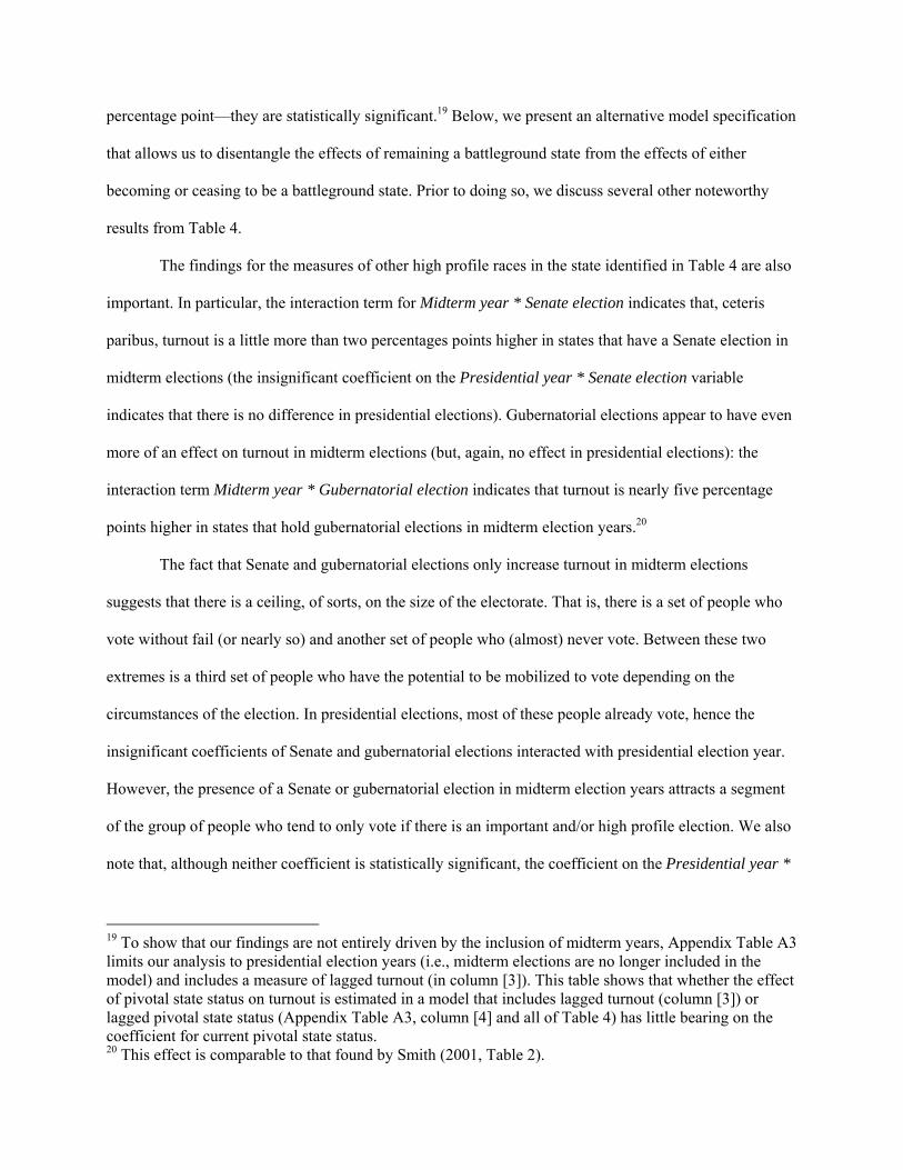
percentage point—they are statistically significant.19 Below, we present an alternative model specification

that allows us to disentangle the effects of remaining a battleground state from the effects of either

becoming or ceasing to be a battleground state. Prior to doing so, we discuss several other noteworthy

results from Table 4.

The findings for the measures of other high profile races in the state identified in Table 4 are also

important. In particular, the interaction term for Midterm year * Senate election indicates that, ceteris

paribus, turnout is a little more than two percentages points higher in states that have a Senate election in

midterm elections (the insignificant coefficient on the Presidential year * Senate election variable

indicates that there is no difference in presidential elections). Gubernatorial elections appear to have even

more of an effect on turnout in midterm elections (but, again, no effect in presidential elections): the

interaction term Midterm year * Gubernatorial election indicates that turnout is nearly five percentage

points higher in states that hold gubernatorial elections in midterm election years.20

The fact that Senate and gubernatorial elections only increase turnout in midterm elections

suggests that there is a ceiling, of sorts, on the size of the electorate. That is, there is a set of people who

vote without fail (or nearly so) and another set of people who (almost) never vote. Between these two

extremes is a third set of people who have the potential to be mobilized to vote depending on the

circumstances of the election. In presidential elections, most of these people already vote, hence the

insignificant coefficients of Senate and gubernatorial elections interacted with presidential election year.

However, the presence of a Senate or gubernatorial election in midterm election years attracts a segment

of the group of people who tend to only vote if there is an important and/or high profile election. We also

note that, although neither coefficient is statistically significant, the coefficient on the Presidential year *

19 To show that our findings are not entirely driven by the inclusion of midterm years, Appendix Table A3 limits our analysis to presidential election years (i.e., midterm elections are no longer included in the model) and includes a measure of lagged turnout (in column [3]). This table shows that whether the effect of pivotal state status on turnout is estimated in a model that includes lagged turnout (column [3]) or lagged pivotal state status (Appendix Table A3, column [4] and all of Table 4) has little bearing on the coefficient for current pivotal state status. 20 This effect is comparable to that found by Smith (2001, Table 2).

Competitive House race interaction is larger than the coefficient on the Midterm year * Competitive

House race term.

3.3 The Effect of Changes in Pivotal State Status on Change in Turnout

As noted above, our longer time series permits a more detailed analysis of the effect of

battleground status on turnout because there are more changes in which states are considered pivotal. We

examine whether becoming a pivotal state results in a larger turnout boost than being a pivotal state in

successive elections in Table 5 (all analysis shown in Table 5 includes only presidential election years).

We regress change in turnout on three indicators of pivotal state status: (1) whether the state became

pivotal since the last presidential election (i.e., new “treatment”); (2) whether the state was pivotal in the

previous presidential election but no longer is in the current presidential election (i.e., old “treatment”);

and (3) whether the state was pivotal in the previous presidential election and still is in the current

presidential election (i.e., new and old “treatment”). The inclusion of these three indicators makes the

omitted reference category states that were not battlegrounds in the previous presidential election and

remain safe in the current presidential election. Thus, the model we estimate is:

(B) ΔTurnouti,t-t-1 = b + b1New Treatmenti,t + b2Old Treatmenti,t + b3New and Old Treatmenti,t + τTt + ψSi + ei,t.

We also include controls for changes in Senate and gubernatorial election status in the same manner as

the changes in pivotal state status variables.

In Table 5, we present the results of this model using VEP in columns (1) and (2) and, so that our

series can include 1980 (which requires a lagged value of turnout in 1976; see footnote 9), Voting Age

Population (VAP) in columns (7) and (8). The other columns in Table 5 present results for slight

modifications to model (B). In particular, columns (3) and (4) [VEP] and (9) and (10) [VAP] omit the

new and old treatment indicator so that the reference category is all states that do not change status (either

because they remain pivotal states or remain not pivotal states). Columns (5) and (6) [VEP] and (11) and

(12) combine the four change in pivotal state status measures into one variable so that new treatment

states are equal to 1, old treatment states are equal to -1, and both (a) new and old treatment states and (b)

states that are not pivotal in successive elections are equal to 0. State fixed effects are included in the odd

numbered columns and excluded from the models in the even numbered columns.


The analysis of change in turnout as a function of changes in battleground status presented in

column 1 shows that states that become pivotal (i.e., are new to the battlefield) experience somewhat21

larger turnout increases than those that maintain their pivotal state status from one election to the next.

Newly pivotal states experience an increase in turnout of about 1.2 percentage points (compared to those

states that are never pivotal); turnout in states that maintain their pivotal status increases by about 65% as

much (around .8 percentage points when compared to those states that are never pivotal). Thus, while

there is a boost in turnout for being a pivotal state a second time, it is not quite as much as the increase the

state experiences when it initially becomes a battleground. These results are robust to the inclusion of

state fixed effects and the use of VAP (which allows the inclusion of 1980). Also of note is that compared

to states that are not pivotal in successive elections, there appears to be a slight persistence (or, habit)

effect caused by states that were part of the battlefield in the previous presidential election but no longer

are in the current election (see columns [1] and [2] and [7] and [8]), although this “old treatment”

coefficient never reaches statistical significance.22

4. Discussion and Conclusion

The perception that one’s vote is pivotal is thought to play an important role in the voter’s

decision-making calculus (Downs 1957; Riker and Ordeshook 1968). Yet, people in the most pivotal

states do not appear to turn out at a substantially higher rate than those in “safe” states—no more than

about two percentage points on average according to our analysis of elections from 1980-2008 (see Table

4). This is the case despite the fact that in addition to being pivotal to the election outcome, campaigns

21 A joint hypothesis test reveals that these coefficients are not statistically distinguishable from one another (p = .43). 22 We note that the results presented in Table 5 are the one instance in which using Shaw’s categorization of battleground states seems to matter. In particular, using Shaw’s measure, any effect of changing battleground status on change in turnout appears to be driven by states that leave the battlefield having lower turnout.

devote massive amounts of resources to stimulate the electorate in battleground states. This finding raises

the question of why battleground status does not have more of an effect on turnout, especially when we

consider that the mere presence of a presidential election boosts turnout by 16 percentage points, or about

eight times as much. One explanation, which finds some support in Table 5, is that the impact on voter

turnout among states that were battlegrounds in the previous election is a bit less than among formerly

safe states that move into the battlefield (although this difference is not statistically significant). Thus,

future work aimed at identifying how changes in battleground status from one election to the next affect

political behaviors and attitudes may be fruitful, particularly in identifying which stimuli (e.g., having

voted in the past [Gerber, Green, and Shachar 2003], registration [Cain and McCue 1985], political

communication [Huber and Arceneaux 2007], etc.) persist over time.

We qualify our conclusions with a number of caveats. First, our finding that the effect of

battleground status is only (in relative terms) about two percentage points does not mean that candidate

and party effort is wasted on battleground states. Indeed, in some instances a small boost in turnout for

one party or the other could mean the difference between victory and defeat. Instead, we emphasize that

the effects of these efforts are quite modest compared with the broader effects of holding a presidential

election.

Second, we note that there does appear to be some variation over time in the effect of

battleground status on turnout. Lipsitz (2009) attributes some of this variation over time to the overall

competitiveness of the election. However, she finds larger effects on turnout for battleground status in

2004 (six percentage points), which turned out to be a less competitive election than 2000 (where she

finds a three percentage point effect). Thus, overall competitiveness cannot be the sole explanation.

Future research may want to consider whether changes in what states become battlegrounds and/or

resource differences (that perhaps vary by party, see Goux 2009) account for such across-year differences.

Another possibility is that there is a greater turnout gap between battleground and safe states in recent

years (especially 2004 and 2008 as indicated by our scatter plots in Figure 1) because voter mobilization

efforts, including more targeted advertising, have become more precise and effective (see Bergan et al.

2005). Indeed, it is difficult to believe that changes in the importance of pivotalness to voters over time

are responsible for greater turnout disparities between battleground and non battleground states in 2004

and 2008. Rather, it is more likely the case that more sophisticated (i.e., targeted) campaigning at least

partially explains the turnout differences between battleground and non battleground states.

With this possibility in mind, we conducted a supplementary analysis in which we included

presidential campaign TV advertising (in GRPs, see footnote 12) as an independent variable in our Table

4, column (1) model specification. If patterns of TV advertising between battleground and non

battleground states have changed over time (e.g., became more targeted at battleground states), it is likely

that the targeting of other campaign activities has also changed in a similar manner, in which case

advertising GRPs will also serve as a proxy for those activities. Given that we only have advertising data

beginning in 1988, the supplementary analysis is only conducted for the years 1988-2008. In order to

provide a more direct comparison to our earlier results, Table 6, column (1) replicates the Table 4, column

(1) specification for this shorter time period. The coefficients for the pivotal state indicator are nearly

identical—2.152 in Table 6 compared to 2.020 in Table 4. Column (2) then presents the results when we

allow the effect of pivotal state status to vary by presidential election year. While all the interaction terms

(pivotal state status with each presidential election year) are positive, only those for 2008 and 2004 are

statistically different from zero. Therefore, there is some indication that there was more of an effect of

battleground status on turnout in the two most recent presidential elections.23


In column (3), we add the advertising data, allowing its effect to vary by presidential election year

as we did battleground status in column (2). Accounting for presidential campaign advertising reduces the

size of the pivotal state indicator by about 40%, suggesting that TV advertising (and other campaign

activities correlated with it) does account for a sizable portion of the battleground effect. Moreover, only

the advertising coefficients for 2008 and 2004 are statistically significant, suggesting that advertising and 23 Tests of the equality of the coefficients indicate that pivotal state status in 2008 and 2004 are not distinguishable from one another (p = .21), but that they are distinguishable from each of the other pivotal state/presidential election year interactions (p < .05).

correlated activities in these two years may primarily account for this portion of the effect.24 Finally, in

column (4) we allow both the effect of pivotal state status and presidential campaign advertising to vary

by presidential election year. Compared to column (2), the size of the coefficients for pivotal state in 2008

and 2004 are reduced by about 25 and 55%, respectively. This serves as some indication that campaign

activities are responsible for some portion of the “battleground effect.” Indeed, if we it were possible to

measure all campaign activities (e.g., party transfers to the states, door-to-door canvassing, etc.), the

“pure” pivotal state effect might approach zero. Therefore, while it is difficult to differentiate increases in

pivotalness from intensive campaigning and mobilization efforts in battleground states, this

supplementary analysis appears to suggest that party efforts are in part responsible for any observed

turnout effects. Moreover, regardless of how much of the battleground effect originates in campaigns, the

aggregate battleground effect is still much less than the effect of factors that affect the entire electorate

during a presidential election, captured by our presidential election indicator, which indicates a boost in

turnout of at least 17 percentages points in Table 6.

Our analysis cannot determine what factors related to presidential elections are not also present in

midterm elections.25 Possibilities range from differences in peoples’ sense of civic duty (Riker and

Ordeshook 1968), factors related to social pressure (Gerber, Green, and Larimer 2008), registration and

mobilization efforts that occur in all states during presidential elections (Gerber and Green 2000;

Rosenstone and Hansen 1993), habit (Gerber, Green, and Shachar 2003), or perhaps simply the

importance of the presidency (compared to other offices) to the American electorate. However, based on

the present analysis, it seems clear that beliefs about the instrumental value of one’s vote cannot explain

these differences. Put another way, in our data, the average difference between turnout in midterm and

presidential elections exceeds 14 percentage points in states like Utah (17.9%), Massachusetts (14.3%),

and Mississippi (23.4%). During the time period we examine these states never come close to being 24 Tests of the equality of the coefficients indicate that only the coefficient for advertising in 2004 is distinguishable from advertising in any other years (p < .05). The coefficient for 2004 is larger than the coefficients for all other years except for 1988 (p = .71). 25 From 1980-2008, there were three instances in which turnout in a presidential election was actually lower than turnout in the previous midterm election: Alaska (1984) and Hawaii (1996 & 2000).

pivotal, making it highly unlikely that these differences can be explained by expectations about the value

of one’s vote to the election outcome.

Last, we note that our measure of pivotalness (i.e., the instrumental value of one’s vote) is based

on objective election outcomes, but it is likely that perceived pivotalness is what is of direct relevance to

prospective voters. If it is the case that residents of non battleground states overestimate their probability

of being pivotal more so than residents of battleground states, then we have underestimated the effect of

pivotalness on turnout. While it seems unlikely that the perceived pivotalness among the electorate would

be skewed in this direction, we encourage future survey research that attempts to measure perceptions of

pivotalness for residents of battleground and non battleground states to see if this assumption is valid.

Our principal concern in this paper was to estimate the effect of battleground status on turnout

and compare the magnitude of this effect to the effect of simply holding a presidential election. We

employed a new modeling strategy that more precisely captures this effect than previous work. Our

finding that the boost in voter turnout associated with presidential elections dwarfs the effect of

battleground status on voter turnout suggests that the reason for the observed surge in turnout in

presidential election years is likely the result of universally held beliefs about the importance of the office

or other factors that affect the entire electorate, rather than beliefs about the instrumentality of one’s vote

or more focused campaign efforts in battleground states. Although precisely what norms are primarily

responsible for the large effects of presidential elections remains to be seen, it is clear that such norms

trump any “extra” motivation to vote—in the form of advertising and campaign visits by the parties

and/or an increased sense that one’s vote is pivotal to the election outcome—induced by residency in a

battleground state.

References

Bartels, Larry M. 1985. “Resource Allocation in a Presidential Campaign.” Journal of Politics 47 (3): 928-936.

Bergan, Daniel E., Alan S. Gerber, Donald P. Green, and Costas Panagopoulos. 2005.

“Grassroots Mobilization and Voter Turnout in 2004.” Public Opinion Quarterly 69 (5): 760-777. Blais, André. 2000. To Vote or Not To Vote? The Merits and Limits of Rational Choice Theory.

Pittsburgh: University of Pittsburgh Press. Brady, Henry. E., and John E. McNulty. 2004. “The Costs of Voting: Evidence from a Natural

Experiment.” Presented at the Annual Meeting of the Society for Political Methodology, Palo Alto, CA.

Brams, Steven J., and Morton D. Davis. 1974. “The 3/2’s Rule in Presidential Campaigning.” American Political Science Review 68 (1): 113-134.

Campbell, James E. 1992. “Forecasting the Presidential Vote in the States.” American Journal of

Political Science 36 (2): 386-407.

Colantoni, Claude S., Terrence J. Levesque, and Peter C. Ordeshook. 1975. “Campaign Resource Allocations under the Electoral College.” American Political Science Review 69 (1): 141-154.

Cox, Gary W., and Michael C. Munger. 1989. “Closeness, Expenditures, and Turnout in the 1982 U.S. House Elections.” American Political Science Review 83 (1): 217-231.

Downs, Anthony. 1957. An Economic Theory of Democracy. New York: Harper & Row. Dyck, Joshua. J., and James G. Gimpel. 2005. “Distance, Turnout, and the Convenience of Voting.”

Social Science Quarterly 86 (3): 531-548. FairVote.org. 2008. “2008’s Shrinking Battleground and Its Start Impact on Campaign Activity.”

December 4. http://fairvote.org/?page=27&pressmode=showspecific&showarticle=230 (July 9, 2009).

Gerber, Alan S., and Donald P. Green. 2000. “The Effect of a Nonpartisan Get-Out-The-Vote Drive: An

Experimental Study of Leafletting. Journal of Politics 62 (3): 846-57. Gerber, Alan S., Donald P. Green, and Ron Shachar. 2003. “Voting May Be Habit-Forming:

Evidence from a Randomized Field Experiment.” American Journal of Political Science 47 (3): 540-550.

Gerber, Alan S., Donald P. Green, and Christopher W. Larimer. 2008. “Social Pressure and Voter

Turnout: Evidence from a Large-Scale Field Experiment.” American Political Science Review 102 (1): 33-48.

Gimpel, James G., Karen M. Kaufmann, and Shanna Pearson-Merkowitz. 2007. “Battleground

States versus Blackout States: The Behavioral Implications of Modern Presidential Campaigns.” Journal of Politics 69 (3): 786-797.

Goux, Darshan. 2009. “Conceptualizing the Battleground State: The Basics.” University of

California, Berkeley. Typescript. Hill, David, and Seth C. McKee. 2005. “The Electoral College, Mobilization, and Turnout in the

2000 Presidential Election.” American Politics Research 33 (5): 700-725. Huang, Taofang, and Daron Shaw. N.d. “Beyond the Battlegrounds? Electoral College Strategies in the

2008 Presidential Election.” Journal of Political Marketing. Forthcoming. Holbrook, Thomas M., and Scott D. McClurg. 2005. “The Mobilization of Core Supporters:

Campaigns, Turnout, and Electoral Composition in United States Presidential Elections.” American Journal of Political Science 49 (4): 689-703.

James, Scott C. and Brian L. Lawson. 1999. “The Political Economy of Voting Rights

Enforcement in America’s Gilded Age: Electoral College Competition, Partisan Commitment, and the Federal Election Law.” American Political Science Review 93 (1): 115-131.

Lipsitz, Keena. 2009. “The Consequences of Battleground and ‘Spectator’ State Residency for Political Participation.” Political Behavior 31 (2): 187-209.

McDonald, Michael P. 2008. “The Return of the Voter: Voter Turnout in the 2008 Presidential

Election.” The Forum 6 (4): article 4. McDonald, Michael P. 2002. “The Turnout Rate Among Eligible Voters for U.S. States, 1980-

2000.” State Politics and Policy Quarterly 2 (2): 199-212. McDonald, Michael P. 2009. “Turnout 1980-2008.” http://elections.gmu.edu/Turnout.html (July

13, 2009). McDonald, Michael P., and Samuel Popkin. 2001. “The Myth of the Vanishing Voter.”American

Political Science Review 95 (4): 963-974.

OpenSecrets.org. 2008. “Banking on Becoming President.” http://www.opensecrets.org/pres08/index.php (July 9, 2009).

Reeves, Andrew, Lanhee Chen, and Tiffany Nagano. “A Reassessment of ‘The Methods behind

the Madness: Presidential Electoral College Strategies, 1988-1996’.” Journal of Politics 66 (2): 616-620.

Riker, William H., and Peter C. Ordeshook. 1968. “A Theory of the Calculus of Voting.” American

Political Science Review 62 (1): 25-42. Rosenstone, Steven J., and John Mark Hansen. 1993. Mobilization, Participation, and

Democracy in America. New York: MacMillian Publishing Company. Shachar, Ron. 2009. “The Political Participation Puzzle and Marketing.” Journal of Marketing

Research. Forthcoming.

Shachar, Ron, and Barry Nalebuff. 1999. “Follow the Leader: Theory and Evidence on Political Participation.” American Economic Review 89 (3): 525-547.

Shaw, Daron. 1999a. “The Effect of TV Ads and Candidate Appearances on Statewide

Presidential Votes, 1988-96.” American Political Science Review 93 (2): 345-361.

Shaw, Daron. 1999b. “The Methods behind the Madness: Presidential Electoral College Strategies, 1988-1996.” Journal of Politics 61 (4): 893-913.

Shaw, Daron. 2006. The Race to 270. Chicago: University of Chicago Press. Smith, Mark A. 2001. “The Contingent Effects of Ballot Initiatives and Candidate Races on

Turnout.” American Journal of Political Science 45 (3): 700-706. Strömberg, David. 2008. “How the Electoral College Influences Campaigns and Policy: The

Probability of Being Florida.” American Economic Review 98 (3): 769-807. Wolak, Jennifer. 2006. “The Consequences of Presidential Battleground Strategies for Citizen

Engagement.” Political Research Quarterly 59 (3): 353-361.

Table A1. List of Pivotal States, by Year

State 1972 1976 1980 1984 1988 1992 1996 2000 2004 2008AK YesAL YesAR Yes Yes YesAZ Yes Yes YesCA Yes Yes YesCO Yes Yes Yes Yes YesCT Yes Yes Yes Yes YesDE Yes Yes Yes YesFL Yes Yes Yes YesGA Yes YesHI Yes Yes YesIA Yes Yes Yes Yes Yes Yes YesIDIL Yes YesIN Yes YesKS YesKY Yes Yes Yes YesLA Yes Yes Yes Yes Yes YesMAMD YesME Yes Yes Yes Yes Yes Yes YesMI Yes Yes Yes Yes Yes Yes YesMN Yes Yes YesMO Yes Yes Yes Yes Yes Yes Yes Yes Yes YesMS YesMT Yes Yes Yes YesNC Yes YesND Yes YesNENH Yes Yes Yes Yes Yes YesNJ Yes Yes Yes Yes Yes YesNM Yes Yes Yes Yes Yes Yes Yes YesNV Yes Yes Yes Yes Yes YesNYOH Yes Yes Yes Yes Yes Yes Yes Yes Yes YesOK YesOR Yes Yes Yes Yes Yes Yes YesPA Yes Yes Yes Yes Yes Yes Yes YesRISCSD Yes YesTN Yes Yes Yes YesTX Yes Yes YesUTVA Yes Yes Yes YesVT Yes Yes Yes Yes YesWA Yes Yes Yes YesWI Yes Yes Yes Yes Yes Yes YesWV Yes YesWYTotal 22 14 15 17 18 21 14 20 18 17

Table A2. Table 4 Robustness: The Effect of Battleground Status on State-level Turnout in Presidential and Midterm Elections

Our Measure, Shaw's Years Shaw's Measure, Shaw's YearsDependent Variable = Turnout in Election as % of VEP (1) (2) (3) (4)

1996-2008 1996-2008 1996-2008 1996-2008Pivotal State, 1=Yes (EC 100), set to 0 in midterm years 2.114

[0.704]**Lagged Pivotal State (t-4), 1=Yes (EC 100), set to 0 in midterm years 0.598

[0.588]Lagged Pivotal State (t-8), 1=Yes (EC 100), set to 0 in midterm years 0.985

[0.540]Pivotal State, 1=Yes (EC 100), midterm based on prev. pres. 1.558

[0.900]Lagged Pivotal State (t-4), 1=Yes (EC 100), midterm based on prev. pres. 1.000

[0.810]Lagged Pivotal State (t-8) 1=Yes (EC 100), midterm based on prev. pres. 0.924

[0.550]Battleground, 1=Yes (Shaw: either party), set to 0 in midterm years 2.367

[0.674]**Lagged Battleground (t-4), 1=Yes (Shaw: either party), set to 0 in midterm years 0.081

[0.608]Lagged Battleground (t-8), 1=Yes (Shaw: either party), set to 0 in midterm years 0.719

[0.474]Battleground, 1=Yes (Shaw: either party), midterm based on prev. pres. 1.012

[0.637]Lagged Battleground (t-4), 1=Yes (Shaw: either party), midterm based on prev. pres. 0.566

[0.593]Lagged Battleground (t-8) 1=Yes (Shaw: either party), midterm based on prev. pres. -0.159

[0.485]Presidential election year 17.866 18.727 18.030 18.536

[2.272]** [2.474]** [2.478]** [2.515]**Pres. year * Prop. House races Comp. (within 10) 0.433 0.690 0.603 0.674

[0.975] [1.002] [0.980] [1.005]Pres. year * Senate election 0.211 0.115 0.259 0.263

[0.297] [0.271] [0.271] [0.280]Pres. year * Gubernatorial election -2.143 -1.951 -2.080 -1.949

[2.215] [2.527] [2.332] [2.536]Midterm year * Prop. House races Comp. (within 10) 2.209 1.891 2.069 1.896

[1.777] [1.945] [1.804] [1.889]Midterm year * Senate election 2.227 2.224 2.210 2.066

[0.625]** [0.639]** [0.621]** [0.624]**Midterm year * Gubernatorial election 5.538 5.183 5.433 5.199

[1.994]** [2.243]* [2.138]* [2.253]*2000 2.234 2.385 2.386 2.473

[0.424]** [0.428]** [0.431]** [0.404]**2002 2.144 2.039 2.143 2.131

[0.689]** [0.694]** [0.689]** [0.684]**2004 8.755 8.843 8.766 8.846

[0.466]** [0.489]** [0.486]** [0.509]**2006 2.900 2.886 2.907 2.891

[0.814]** [0.812]** [0.812]** [0.806]**2008 9.944 10.026 10.219 10.177

[0.645]** [0.647]** [0.710]** [0.713]**Constant 31.390 31.041 31.246 31.078

[2.155]** [2.336]** [2.330]** [2.390]**State Fixed Effects Yes Yes Yes YesYear Fixed Effects Yes Yes Yes YesObservations 350 350 350 350R-squared 0.930 0.930 0.930 0.930F test: Joint Significance of BG 3.490 1.620 5.900 1.650Prob > F 0.020 0.200 0.000 0.190Note : OLS regression coefficients with robust standard errors clustered by state in brackets. State fixed effects not reported to save space. Columns (1) and (3) correspond to Table 4, column (4); columns (2) and (4) correspond to Table 4, column (8)."Pivotal State" is equal to 1 if the closeness of a state's two-party vote share places it within 100 electoral votes of being decisive, and is explained in greater detail in the text.Shaw's measure of "battleground" status is equal to 1 if either party reports that the state was a battleground, and is explained in greater detail in the text and in Shaw (1999b, 2006) and Huang and Shaw (forthcoming).* significant at 5%; ** significant at 1%

Table A3. The Effect of being a Pivotal State on State-level Turnout in Presidential Elections, 1980-2008

Dependent Variable = Turnout in Election as % of VEP (1) (2) (3) (4)1980-2008 1984-2008 1984-2008 1984-2008

Pivotal State, 1=Yes (EC 100) 1.266 1.427 1.137 1.211[0.468]** [0.535]* [0.381]** [0.450]**

Lagged Pivotal State (t-4), 1=Yes (EC 100) 0.841[0.384]*

Lagged TO (VEP), previous election 0.557[0.077]**

Proportion House races decided by 10 points or less 1.338 0.867 0.871 0.844[0.757] [0.699] [0.588] [0.675]

Senate election year 0.254 0.333 0.280 0.348[0.227] [0.220] [0.294] [0.222]

Gubernatorial election year 3.896 3.187 1.574 3.342[0.672]** [0.606]** [0.347]** [0.503]**

1984 0.515[0.351]

1988 -1.438 -1.997 -2.296 -2.025[0.362]** [0.269]** [0.368]** [0.265]**

1992 3.904 3.398 4.270 3.369[0.531]** [0.458]** [0.463]** [0.463]**

1996 -2.728 -3.215 -5.539 -3.321[0.641]** [0.541]** [0.544]** [0.535]**

2000 -0.337 -0.887 0.651 -0.851[0.715] [0.594] [0.493] [0.596]

2004 6.137 5.566 5.740 5.491[0.714]** [0.617]** [0.418]** [0.611]**

2008 7.347 6.811 3.441 6.767[0.949]** [0.845]** [0.663]** [0.830]**

Constant 50.592 51.385 23.218 51.324[0.435]** [0.398]** [3.976]** [0.385]**

State Fixed Effects Yes Yes Yes YesYear Fixed Effects Yes Yes Yes YesObservations 400 350 350 350R-squared 0.890 0.900 0.930 0.900F test: Joint Significance of BG 3.870Prob > F 0.030Note : OLS regression coefficients with robust standard errors clustered by state in brackets. State fixed effects not reported to save space. VEP not available prior to 1980. Models using VAP (and, therefore, include 1980) produce similar results."Pivotal State" is equal to 1 if the closeness of a state's two-party vote share places it within 100 electoral votes ofbeing decisive, and is explained in greater detail in the text. * significant at 5%; ** significant at 1%

Table A4. Table 5 Robustness: Effect of Changes in Battleground Status on Change in State-level Turnout in Presidential Elections

Our Measure, Shaw's Years Shaw's Measure, Shaw's YearsDependent Variable = Change in Presidential Election Turnout as a % of VEP (1) (2) (3) (4) (5) (6)

1992-2008 1992-2008 1992-2008 1992-2008 1992-2008 1992-2008Became Pivotal state since last Pres, EC 100 (1=Yes) 0.913 0.403 New "treatment" [0.651] [0.614]No longer Pivotal state since last Pres, EC 100 (1=Yes) 0.416 0.187 Old "treatment" (persistence) [0.492] [0.552]Was Pivotal state last Pres. and still pivotal, EC 100 (1=Yes) 0.917 New and old "treatment" [0.647]Change in Pivotal State Status, EC 100 (-1,0,1) 0.117

[0.426]Became Battleground state since last Pres, Shaw (1=Yes) -0.039 -0.117 New "treatment" [0.787] [0.663]No longer Battleground state since last Pres, Shaw (1=Yes) -1.648 -1.843 Old "treatment" (persistence) [0.603]** [0.578]**Was Battleground last Pres and still Battleground, Shaw (1=Yes) 0.368 New and old "treatment" [0.654]Change in Battleground Status, Shaw (-1,0,1) 0.858

[0.417]*Senate race this time, not last Pres. (1=Yes) 2.621 0.750 2.596 0.915

[1.345] [0.444] [1.297] [0.416]*No Senate race this time, Yes last Pres. (1=Yes) -0.230 -0.080 -0.071 0.031

[0.510] [0.540] [0.473] [0.500]Was Senate last pres and still Senate (1=Yes) -2.039 -1.786

[1.265] [1.270]Change in Senate Election from last Pres. (-1,0,1) 0.405 0.411

[0.266] [0.257]No governor race this time, Yes last Pres. (1=Yes) -1.339 -1.359 -1.412 -1.446

[0.557]* [0.555]* [0.550]* [0.536]**Was governor last Pres and still governor (1=Yes) 2.393 2.328 2.270 2.257

[0.586]** [0.589]** [0.573]** [0.565]**Change in Governor Election from last Pres. (-1,0,1) 1.873 1.856

[0.545]** [0.537]**1996 -12.283 -12.345 -12.392 -12.402 -12.384 -12.364

[0.631]** [0.643]** [0.632]** [0.620]** [0.643]** [0.649]**2000 -3.060 -3.082 -3.182 -2.989 -2.978 -3.141

[0.530]** [0.538]** [0.512]** [0.508]** [0.508]** [0.508]**2004 0.897 0.844 0.762 0.643 0.642 0.802

[0.549] [0.556] [0.539] [0.593] [0.590] [0.550]2008 -4.210 -4.196 -4.313 -4.306 -4.256 -4.185

[0.603]** [0.633]** [0.600]** [0.570]** [0.590]** [0.574]**Constant 6.401 6.329 6.601 6.358 6.280 6.553

[0.430]** [0.467]** [0.360]** [0.389]** [0.425]** [0.365]**State Fixed Effects Yes Yes Yes Yes Yes YesYear Fixed Effects Yes Yes Yes Yes Yes YesObservations 250 250 250 250 250 250R-squared 0.830 0.820 0.820 0.830 0.830 0.830Note : OLS regression coefficients with standard errors clustered by state in brackets. State fixed effects not reported to save space.Columns (1) & (4), (2) & (5), and (3) & (6) correspond to Table 6, columns (1), (3), and (5), respectively."Pivotal State" is equal to 1 if the closeness of a state's two-party vote share places it within 100 electoral votes of being decisive, and is explained in greater detail in the text. Shaw's measure of "battleground" status is equal to 1 if either party reports that the state was a battleground, and is explained in greater detail in the text and in Shaw (1999b, 2006)and Huang and Shaw (forthcoming).Change in Presidential Election Turnout = (%TO at t - %TO at t-4).The omitted, reference category for the change in pivotal status indicators are states that were not pivotal in the previous presidential election (t-4) and still are not pivotal in the currentpresidential election (t).* significant at 5%; ** significant at 1%

BB

B BB

B

B

B

BB

B

S

S

SS

SS

S

S

S

S

S

S

S

S

S

S

S

S

S

S

S

S

S

S

S

S

S

S

S

S

S

S

S

SS

SS

S

S

2030

4050

6070

80T

urno

ut in

Pre

side

ntia

l Ele

ctio

n (%

VE

P)

20 30 40 50 60 70 80Turnout in Previous Midterm Election (% VEP)

1988

B

B

B

B

B

BB

B

B

BB

B

B

B

S

S

SS

S

S

SS

S

S

S

S

SS

S

S

S

S

S

S

S

S

S

S

S

S

S

S

S S

S

S

S

S

S

S

2030

4050

6070

80T

urno

ut in

Pre

side

ntia

l Ele

ctio

n (%

VE

P)


1992

B

BBB

B

B

B

B

BB

BB

B

BS

S

S

S

S

S

S

SS

SS

S

S

S

S

S

S

S

S

S

S

S

S

S

S

S

S

S

S

S

S

S

S

S

SS

2030

4050

6070

80T

urno

ut in

Pre

side

ntia

l Ele

ctio

n (%

VE

P)


1996

B

B

B

B

B

B

B

B

B

B

B

B

B

B

B

S

S

S

SS

SS

SS

SS

S

S

S

S S

S

S

S

S

S

SS

S

S

S

S

S

S

S

S

S

S

S

S

2030

4050

6070

80T

urno

ut in

Pre

side

ntia

l Ele

ctio

n (%

VE

P)


2000

B

B

B

B

B

B

B

B

B

B

B

B

B

B

B

S

S

S S

S

SSS

S

S

SS

S

SS

SS

S

S

SSS

S S

S

S S

S

S

SS

S

S

S

S

2030

4050

6070

80T

urno

ut in

Pre

side

ntia

l Ele

ctio

n (%

VE

P)


2004

BB

BB

B

B

B

BB

B

S

S

SS

S

SS

S

S

SS

S

S

S

S

S

S

SS

S

S

S

S

S

S

S S

S

S

S

S

S

SS

S

SS

S

S

S

2030

4050

6070

80T

urno

ut in

Pre

side

ntia

l Ele

ctio

n (%

VE

P)


2008

Note: Solid lines are linear regressions in battleground (B) states as defined by Shaw (1999b, 2006) and Huang and Shaw (forthcoming)− one or both parties said state was battleground. Dashed lines are linear regressions in safe (S) states.

as a Function of Turnout in the Previous Midterm Election, 1988−2008Figure A1. Presidential Election Turnout in Battleground and Safe States

Table 1. Previous Research on the Effect of Battleground Status on Voter Turnout in Presidential Elections, 1980-2008

Increase in turnout rate for full rangeArticle Election(s) Measure of "Battleground" State (range) Dependent Variable (range) of "battleground" measure (p-value)

Lipsitz (2009) 1988-2004 Shaw (1999b, 2006) (0, 4) [Note 1] turnout rate (0, 1) +.04 (p<.10)

McDonald (2008) 2008 Candidate visits in last 2 weeks of election (0, 1) % turnout (0, 100) +.04 (none, descriptive)

Wolak (2006) 1992-2000 Campaign advertising (GRPs) and candidate visits ANES "plans to vote" (0, 1=Yes) .009 and .002 (not stat. sig.)

Bergan et al. (2005) 2004 CNN state rankings (0,1) % turnout (0, 100) +.05 (p<.001)

Holbrook & McClurg (2005) 1992-2000 Closeness based on pre-election polls (0, 1) change in turnout (-100, 100) .002 (not stat. sig.)

Hill & McKee (2005) 2000 Shaw (2006) (0, 1) [Note 1] % turnout (0, 100) +.015 and +.001 (p<.05) [Note 2]

Shachar & Nalebuff (1999) 1980-1988 Predicted closeness (based on Campbell 1992) (-1, 0) turnout rate (0, 1) +.17 (p<.01)

Note : Wolak's (2006) analysis is of self-reported voter turnout on the American National Election Study (ANES); all other studies use state-level turnout statistics. Shachar and Nalebuff's study extends back to 1948, but our analysis focuses on the years 1980-2008 in order to have comparable estimates of state-level voter turnout based on the state's voting eligible population (VEP, see McDonald 2002; McDonald and Popkin 2001).Note 1: Shaw (1999b, 2006) identifies battleground states based upon information given to him by campaign consultants involved in planning the Electoral College strategies of the presidential candidates. See text and Shaw (1999b, 2006) for further details.Note 2: Hill & McKee's (2005) analysis proceeds in two steps. First, they estimate the effect of battleground states on campaign advertising and candidate visits, and then estimate the effect of these two variables on turnout. The figures reported in this table were obtained from their estimates of the indirect effect of battleground status (through campaign advertising [.015] and candidate visits [.001]) on voter turnout (2005, footnotes 25 & 26).

Table 2. Media Spending and Candidate Visits in Battleground (BG) and Non Battleground (NBG) States, 1988-2008

Pivotal State Measure a Shaw's Measure b

BG NBGDifference

BG NBGDifference

1988 All States (BG-NBG) (BG-NBG)Total Advertising (GRPs in 100s)c 38 55 29 26 67 30 37

[23] [21] [18] [18] [16]Total Visits 4.7 8.2 2.7 5.5 14.5 1.9 12.7

[7.1] [9.0] [5.0] [8.7] [3.0]Numer of States 50 18 32 11 39

BG NBGDifference

BG NBGDifference

1992 All States (BG-NBG) (BG-NBG)Total Advertising (GRPs in 100s) 81 124 49 75 157 51 106

[55] [54] [25] [24] [27]Total Visits 3.6 5.3 2.4 2.9 7.6 2.1 5.5

[3.8] [4.6] [2.6] [4.4] [2.2]Numer of States 50 21 29 14 36

BG NBGDifference

BG NBGDifference


[44] [47] [34] [42] [29]Total Visits 4.8 6.9 4.0 2.9 10.4 2.7 7.7

[5.9] [5.1] [6.1] [7.7] [3.2]Numer of States 50 14 36 14 36

BG NBGDifference

BG NBGDifference


[154] [146] [17] [132] [66]Total Visits 4.7 9.3 1.6 7.7 11.1 1.9 9.2

[7.3] [8.1] [4.7] [8.2] [4.7]Numer of States 50 20 30 15 35

BG NBGDifference

BG NBGDifference


[80] [88] [34] [63] [28]Total Visits 4.3 11.2 0.5 10.8 12.6 0.8 11.8

[8.9] [12.0] [1.5] [12.7] [2.0]Numer of States 50 18 32 15 35

BG NBGDifference

BG NBGDifference


[251] [283] [40] [256] [109]Total Visits 5.5 12.5 1.9 10.6 16.3 2.8 13.5

[7.1] [7.5] [3.3] [6.9] [4.0]Numer of States 50 17 33 10 40Note : cell entries are means with standard deviations in brackets.a "Pivotal State" is equal to 1 if the closeness of a state's two-party vote share places it within 100 electoral votes of being decisive, and is explained in greater detail in the text. b Shaw's measure of "battleground" status is equal to 1 if either party reports that the state was a battleground, and is explained in greater detail in the text and in Shaw (1999b, 2006)and Huang and Shaw (forthcoming).c Campaign advertising and candidate visit data obtained from Shaw (1999a, 2006) and Huang and Shaw (forthcoming). For 1988, 1992, & 1996 Shaw's (1999a) GRP figures do not include spending by the Republican and Democratic National Committees; 2000 & 2004 do (Shaw 2006). Candidate visits for 2000 & 2004 do not include private fund-raising events and vacation days (Shaw 2006); the three earlier years do count such events if the campaigns recorded them as "appearances" (Shaw 1999a, 2006). Part of the reason for the sharp increase in total spending and visits in 2008 is that the estimates include part of the primary season, beginning in mid-June rather than August (Huang and Shaw forthcoming).

Table 3. Summary Statistics for Model Variables, Overall and by Year

Variable 1972-2008 1972 1976 1980 1984 1988 1992 1996 2000 2004 2008Turnout as % of Voting Eligible Population (VEP 57.844 56.242 56.734 54.663 60.266 53.401 55.829 62.175 63.440

[7.2526] [7.3727] [6.2886] [6.2711] [6.7767] [6.1582] [6.5007] [6.2948] [5.8126]Turnout as % of Voting Age Population (VAP) 55.196 56.132 55.151 54.809 54.993 52.705 57.657 50.670 52.588 58.149 59.120

[7.5316] [8.751] [7.4782] [7.5344] [6.5169] [6.5657] [7.2136] [6.6412] [6.97] [7.0819] [6.5048]Change in Pres. Turnout from Previous Pres. Election (VEP) 1.028 0.492 -2.071 5.604 -6.865 2.428 6.346 1.265

[4.8429] [2.2027] [1.741] [2.5442] [2.5435] [2.7405] [2.197] [2.8188]Change in Pres. Turnout from Previous Pres. Election (VAP) 0.321 -1.107 -0.342 0.184 -2.288 4.952 -6.987 1.918 5.561 0.971

[4.355] [3.3539] [2.7818] [2.0854] [1.7105] [2.4841] [2.5256] [2.5346] [2.0956] [2.6683]Pivotal State, 1=Yes (EC 100), set to 0 in midterm yearsa 0.352 0.440 0.280 0.300 0.340 0.360 0.420 0.280 0.400 0.360 0.340

[.4781] [.5014] [.4536] [.4629] [.4785] [.4849] [.4986] [.4536] [.4949] [.4849] [.4785]Battleground, 1=Yes (Shaw: either party), set to 0 in midterm yearsb 0.263 0.220 0.280 0.280 0.300 0.300 0.200

[.4412] [.4185] [.4536] [.4536] [.4629] [.4629] [.4041]Senate election year 0.667 0.660 0.680 0.640 0.660 0.680 0.660 0.680 0.680 0.660

[.4719] [.4785] [.4712] [.4849] [.4785] [.4712] [.4785] [.4712] [.4712] [.4785]Gubernatorial election year 0.238 0.260 0.260 0.260 0.240 0.240 0.220 0.220 0.220 0.220

[.4262] [.4431] [.4431] [.4431] [.4314] [.4314] [.4185] [.4185] [.4185] [.4185]Proportion of House races decided by 10 points or less 0.147 0.169 0.179 0.167 0.120 0.068 0.202 0.223 0.133 0.075 0.139

[.2097] [.2319] [.2394] [.2062] [.1446] [.1108] [.2244] [.2624] [.2208] [.1769] [.195]Observations 500 50 50 50 50 50 50 50 50 50 50

Variable 1974-2006 1974 1978 1982 1986 1990 1994 1998 2002 2006Turnout as % of Voting Eligible Population (VEP 42.433 44.573 41.458 41.534 43.279 40.377 42.502 43.350

[8.1215] [8.2629] [8.5141] [8.8773] [8.0344] [7.9514] [7.0457] [7.7828]Turnout as % of Voting Age Population (VAP) 40.407 43.304 40.107 39.911 41.210 38.099 39.845 40.433

[8.2299] [8.2379] [8.6098] [8.8543] [8.0311] [7.9126] [7.3696] [8.09]Change in Pres. Turnout from Previous Pres. Election (VEP)

Change in Pres. Turnout from Previous Pres. Election (VAP)

Pivotal State, 1=Yes (EC 100), set to 0 in midterm yearsa 0.000 0.000 0.000 0.000 0.000 0.000 0.000 0.000 0.000 0.000[0] [0] [0] [0] [0] [0] [0] [0] [0] [0]

Battleground, 1=Yes (Shaw: either party), set to 0 in midterm yearsb 0.000 0.000 0.000 0.000 0.000 0.000[0] [0] [0] [0] [0] [0]

Senate election year 0.675 0.660 0.680 0.680 0.680 0.680 0.680 0.680 0.660[.469] [.4785] [.4712] [.4712] [.4712] [.4712] [.4712] [.4712] [.4785]

Gubernatorial election year 0.720 0.720 0.720 0.720 0.720 0.720 0.720 0.720 0.720[.4496] [.4536] [.4536] [.4536] [.4536] [.4536] [.4536] [.4536] [.4536]

Proportion of House races decided by 10 points or less 0.173 0.244 0.140 0.216 0.121 0.142 0.236 0.137 0.128 0.190[.2239] [.2519] [.1424] [.2552] [.1586] [.1912] [.2613] [.197] [.222] [.2698]

Observations 450 50 50 50 50 50 50 50 50 50Note : Table entries are averages with standard deviations in brackets. a "Pivotal State" is equal to 1 if the closeness of a state's two-party vote share places it within 100 electoral votes of being decisive, and is explained in greater detail in the text. b Shaw's measure of "battleground" status is equal to 1 if either party reports that the state was a battleground, and is explained in greater detail in the text and in Shaw (1999b, 2006).

Table 4. The Effect of Being a Pivotal State on State-level Turnout in Presidential and Midterm Elections, 1980-2008

Dependent Variable = Turnout in Election as % of VEP (1) (2) (3) (4) (5) (6) (7) (8)1980-2008 1980-2008 1980-2008 1980-2008 1980-2008 1980-2008 1980-2008 1980-2008

Pivotal State, 1=Yes (EC 100), set to 0 in midterm years 2.020 1.565 1.584[0.554]** [0.441]** [0.455]**

Lagged Pivotal State (t-4), 1=Yes (EC 100), set to 0 in midterm years 1.724 1.060 0.821[0.503]** [0.351]** [0.306]*

Lagged Pivotal State (t-8), 1=Yes (EC 100), set to 0 in midterm years 0.785[0.317]*

Pivotal State, 1=Yes (EC 100), midterm based on prev. pres. 0.903 0.724 0.834[0.445]* [0.409] [0.431]

Lagged Pivotal State (t-4), 1=Yes (EC 100), midterm based on prev. pres. 0.911 0.741 0.650[0.414]* [0.378] [0.365]

Lagged Pivotal State (t-8) 1=Yes (EC 100), midterm based on prev. pres. 0.653[0.372]

Presidential election year 16.591 16.622 16.390 16.111 17.169 17.145 17.157 17.216[1.774]** [1.806]** [1.787]** [1.846]** [1.777]** [1.787]** [1.774]** [1.763]**

Pres. year * Prop. House races Comp. (within 10) 0.724 0.748 0.693 0.691 0.814 0.788 0.776 0.774[0.927] [0.983] [0.930] [0.956] [0.980] [0.998] [0.973] [0.995]

Midterm year * Prop. House races Comp. (within 10) 1.396 1.389 1.403 1.420 1.361 1.193 1.220 1.223[1.076] [1.083] [1.077] [1.076] [1.125] [1.112] [1.136] [1.133]

Pres. year * Senate election 0.247 0.284 0.269 0.250 0.240 0.260 0.251 0.232[0.226] [0.233] [0.229] [0.226] [0.223] [0.227] [0.225] [0.227]

Midterm year * Senate election 2.316 2.318 2.320 2.325 2.320 2.310 2.319 2.330[0.426]** [0.427]** [0.427]** [0.428]** [0.426]** [0.423]** [0.423]** [0.427]**

Pres. year * Gubernatorial election -1.196 -1.078 -1.118 -1.120 -1.218 -1.209 -1.215 -1.235[1.810] [1.849] [1.811] [1.811] [1.868] [1.869] [1.863] [1.858]

Midterm year * Gubernatorial election 4.923 4.880 4.898 4.872 4.917 4.931 4.927 4.960[1.610]** [1.633]** [1.611]** [1.620]** [1.652]** [1.648]** [1.645]** [1.637]**

1984 0.455 0.504 0.452 0.580 0.504 0.521 0.495 0.596[0.366] [0.334] [0.347] [0.332] [0.325] [0.319] [0.323] [0.315]

1986 -2.896 -2.898 -2.892 -2.888 -2.950 -2.929 -2.958 -2.846[0.801]** [0.801]** [0.802]** [0.802]** [0.805]** [0.808]** [0.808]** [0.793]**

1988 -1.647 -1.624 -1.684 -1.562 -1.571 -1.574 -1.609 -1.519[0.378]** [0.408]** [0.404]** [0.388]** [0.357]** [0.373]** [0.373]** [0.376]**

1990 -2.849 -2.852 -2.846 -2.843 -2.921 -2.914 -2.952 -2.852[0.932]** [0.932]** [0.933]** [0.935]** [0.924]** [0.920]** [0.920]** [0.899]**

1992 3.733 3.839 3.705 3.801 3.864 3.900 3.827 3.886[0.547]** [0.519]** [0.543]** [0.538]** [0.517]** [0.506]** [0.518]** [0.514]**

1994 -1.236 -1.238 -1.234 -1.232 -1.358 -1.300 -1.381 -1.311[0.774] [0.775] [0.774] [0.774] [0.798] [0.785] [0.802] [0.788]

1996 -2.883 -3.161 -3.035 -2.939 -2.911 -3.055 -3.016 -2.950[0.631]** [0.626]** [0.627]** [0.619]** [0.622]** [0.621]** [0.621]** [0.615]**

1998 -3.999 -4.001 -3.996 -3.992 -3.998 -4.138 -4.104 -4.027[0.873]** [0.873]** [0.873]** [0.873]** [0.883]** [0.867]** [0.874]** [0.856]**

2000 -0.637 -0.430 -0.590 -0.576 -0.523 -0.434 -0.507 -0.505[0.725] [0.701] [0.716] [0.714] [0.719] [0.706] [0.713] [0.713]

2002 -1.862 -1.864 -1.859 -1.855 -1.970 -1.875 -1.952 -1.939[0.877]* [0.877]* [0.878]* [0.879]* [0.875]* [0.864]* [0.870]* [0.868]*

2004 5.831 5.752 5.732 5.884 5.906 5.848 5.824 5.932[0.729]** [0.733]** [0.719]** [0.711]** [0.743]** [0.744]** [0.735]** [0.725]**

2006 -1.054 -1.056 -1.051 -1.048 -1.124 -1.164 -1.193 -1.074[0.960] [0.961] [0.960] [0.961] [0.971] [0.963] [0.971] [0.950]

2008 7.095 7.044 7.031 7.080 7.141 7.104 7.088 7.116[0.931]** [0.923]** [0.918]** [0.918]** [0.946]** [0.941]** [0.933]** [0.932]**

Constant 35.102 35.110 35.194 35.278 34.803 34.820 34.771 34.576[1.697]** [1.727]** [1.708]** [1.723]** [1.712]** [1.726]** [1.717]** [1.666]**

State Fixed Effects Yes Yes Yes Yes Yes Yes Yes YesYear Fixed Effects Yes Yes Yes Yes Yes Yes Yes YesObservations 749 749 749 749 749 749 749 749R-squared 0.890 0.890 0.890 0.890 0.890 0.890 0.890 0.890F test: Joint Significance of BG 6.860 4.580 2.950 2.240Prob > F 0.000 0.010 0.060 0.100Note : OLS regression coefficients with robust standard errors clustered by state in brackets. State fixed effects not reported to save space. Louisiana did not hold a general election in 1982, explaining the 1missing observation."Pivotal State" is equal to 1 if the closeness of a state's two-party vote share places it within 100 electoral votes of being decisive, and is explained in greater detail in the text. * significant at 5%; ** significant at 1%

Table 5. The Effect of Changes in Pivotal State Status on Change in State-level Turnout in Presidential Elections

Dependent Variable = Change in Presidential Election Turnout (1) (2) (3) (4) (5) (6) (7) (8) (9) (10) (11) (12)VEP: 1984-

2008VEP: 1984-

2008VEP: 1984-

2008VEP: 1984-

2008VEP: 1984-

2008VEP: 1984-

2008VAP: 1980-

2008VAP: 1980-

2008VAP: 1980-

2008VAP: 1980-

2008VAP: 1980-

2008VAP: 1980-

2008Became Pivotal state since last Pres, EC 100 (1=Yes) 1.261 1.229 0.920 1.005 1.295 1.128 1.018 0.951 New "treatment" [0.459]** [0.389]** [0.439]* [0.387]* [0.400]** [0.354]** [0.369]** [0.343]**No longer Pivotal state since last Pres, EC 100 (1=Yes) 0.481 0.300 0.195 0.108 0.555 0.308 0.290 0.099 Old "treatment" (persistence) [0.368] [0.330] [0.362] [0.328] [0.356] [0.311] [0.355] [0.308]Was Pivotal state last Pres. and still pivotal, EC 100 (1=Yes) 0.846 0.702 0.801 0.672 New and old "treatment" [0.436] [0.249]** [0.343]* [0.238]**Change in Pivotal State Status, EC 100 (-1,0,1) 0.392 0.460 0.396 0.433

[0.291] [0.264] [0.253] [0.232]Senate race this time, not last Pres. (1=Yes) 2.146 1.499 0.648 0.576 2.288 2.079 0.842 0.822

[1.481] [1.443] [0.328] [0.321] [0.940]* [0.916]* [0.311]** [0.297]**No Senate race this time, Yes last Pres. (1=Yes) -0.025 -0.064 0.052 0.004 -0.044 -0.111 0.026 -0.034

[0.384] [0.361] [0.405] [0.378] [0.337] [0.312] [0.348] [0.325]Was Senate last pres and still Senate (1=Yes) -1.582 -0.992 -1.536 -1.342

[1.415] [1.387] [0.885] [0.862]Change in Senate Election from last Pres. (-1,0,1) 0.291 0.287 0.407 0.433

[0.202] [0.191] [0.186]* [0.173]*No governor race this time, Yes last Pres. (1=Yes) -0.970 -1.813 -1.000 -1.952 -0.935 -1.637 -0.971 -1.763

[0.412]* [0.294]** [0.423]* [0.300]** [0.441]* [0.278]** [0.445]* [0.287]**Was governor last Pres and still governor (1=Yes) 0.278 -0.421 0.316 -0.445 0.388 -0.286 0.347 -0.325

[0.428] [0.365] [0.466] [0.384] [0.699] [0.338] [0.667] [0.360]Change in Governor Election from last Pres. (-1,0,1) 0.807 1.583 0.762 1.397

[0.368]* [0.337]** [0.360]* [0.349]**1984 0.438 0.463 0.443 0.461 0.542 0.543

[0.565] [0.527] [0.555] [0.521] [0.565] [0.529]1988 -2.486 -2.484 -2.439 -2.434 -2.556 -2.539 -1.947 -1.945 -1.894 -1.897 -1.932 -1.919

[0.503]** [0.459]** [0.499]** [0.463]** [0.496]** [0.458]** [0.496]** [0.455]** [0.486]** [0.452]** [0.490]** [0.455]**1992 5.097 5.077 5.134 5.116 5.087 5.085 5.196 5.201 5.234 5.228 5.278 5.277

[0.490]** [0.451]** [0.486]** [0.454]** [0.502]** [0.465]** [0.484]** [0.446]** [0.479]** [0.448]** [0.476]** [0.446]**1996 -7.205 -7.215 -7.202 -7.199 -7.276 -7.248 -6.574 -6.570 -6.564 -6.559 -6.550 -6.531

[0.454]** [0.419]** [0.461]** [0.426]** [0.455]** [0.423]** [0.544]** [0.503]** [0.536]** [0.498]** [0.541]** [0.505]**2000 2.026 1.975 2.043 2.005 1.888 1.882 2.281 2.239 2.303 2.257 2.220 2.216

[0.525]** [0.478]** [0.525]** [0.482]** [0.500]** [0.460]** [0.526]** [0.488]** [0.523]** [0.487]** [0.528]** [0.492]**2004 5.980 5.936 5.987 5.961 5.874 5.880 5.955 5.931 5.968 5.942 5.934 5.937

[0.529]** [0.474]** [0.533]** [0.491]** [0.519]** [0.481]** [0.564]** [0.513]** [0.564]** [0.521]** [0.558]** [0.521]**2008 0.916 0.886 0.976 0.949 0.791 0.795 1.395 1.356 1.462 1.418 1.345 1.348

[0.476] [0.442] [0.488] [0.451]* [0.470] [0.436] [0.538]* [0.507]* [0.559]* [0.522]** [0.568]* [0.531]*Constant 0.774 0.069 0.794 0.203 1.252 0.485 0.255 -0.770 0.246 -0.649 0.695 -0.359

[0.404] [0.449] [0.417] [0.445] [0.297]** [0.323] [0.366] [0.411] [0.381] [0.412] [0.366] [0.385]State Fixed Effects Yes No Yes No Yes No Yes No Yes No Yes NoYear Fixed Effects Yes Yes Yes Yes Yes Yes Yes Yes Yes Yes Yes YesObservations 350 350 350 350 350 350 400 400 400 400 400 400R-squared 0.800 0.770 0.800 0.760 0.790 0.760 0.770 0.740 0.770 0.730 0.760 0.720Note : OLS regression coefficients with standard errors clustered by state in brackets. State fixed effects included in odd numbered columns, but not reported to save space."Pivotal State" is equal to 1 if the closeness of a state's two-party vote share places it within 100 electoral votes of being decisive, and is explained in greater detail in the text. Change in Presidential Election Turnout = (TO % at t - TO % at t-4).The omitted, reference category for the change in pivotal status indicators are states that were not pivotal in the previous presidential election (t-4) and still are not pivotal in the current presidential election (t).* significant at 5%; ** significant at 1%

Table 6. The Effect of Being a Pivotal State on State-level Turnout in Presidential and Midterm Elections, 1988-2008, Controlling for Total Advertising in the State

Dependent Variable = Turnout in Election as % of VEP (1) (2) (3) (4)

Just BG IndicatorBG Indicator * Pres. Years

BG Indicator Plus Total GRPs

BG Indicator * Pres. Years Plus

Total GRPsPivotal State, 1=Yes (EC 100), set to 0 in midterm years 2.152 1.243

[0.623]** [0.812]Pivotal State 2008 5.325 3.940

[1.217]** [1.833]*Pivotal State 2004 3.992 1.816

[1.032]** [1.101]Pivotal State 2000 1.824 1.164

[0.964] [1.977]Pivotal State 1996 1.065 1.038

[0.875] [0.844]Pivotal State 1992 0.476 0.659

[0.978] [1.882]Pivotal State 1988 0.730 0.028

[0.838] [0.914]Total GRPs 2008 (in 100s) 0.008 0.004

[0.002]** [0.003]Total GRPs 2004 (in 100s) 0.022 0.020

[0.005]** [0.005]**Total GRPs 2000 (in 100s) 0.003 0.003

[0.004] [0.006]Total GRPs 1996 (in 100s) 0.003 0.004

[0.008] [0.008]Total GRPs 1992 (in 100s) -0.004 -0.001

[0.010] [0.016]Total GRPs 1988 (in 100s) 0.014 0.028

[0.024] [0.022]Presidential election year 17.711 18.305 17.640 17.546

[2.053]** [1.972]** [2.133]** [2.095]**Pres. year * Prop. House races Comp. (within 10) -0.438 -0.270 -0.379 -0.329

[0.812] [0.794] [0.818] [0.806]Pres. year * Senate election 0.570 0.569 0.670 0.646

[0.284] [0.307] [0.285]* [0.297]*Pres. year * Gubernatorial election -1.436 -1.525 -1.452 -1.493

[2.064] [2.007] [2.077] [2.026]Midterm year * Prop. House races Comp. (within 10) 0.787 0.773 0.819 0.794

[1.357] [1.342] [1.360] [1.363]Midterm year * Senate election 2.167 2.174 2.168 2.171

[0.517]** [0.518]** [0.519]** [0.520]**Midterm year * Gubernatorial election 5.241 5.336 5.488 5.497

[1.832]** [1.777]** [1.844]** [1.798]**1992 5.522 5.691 6.433 6.498

[0.437]** [0.510]** [0.967]** [0.984]**1994 1.671 1.672 1.668 1.670

[0.941] [0.945] [0.948] [0.952]1996 -1.050 -1.286 -0.789 -0.664

[0.511]* [0.692] [1.119] [1.095]1998 -1.152 -1.152 -1.152 -1.152

[0.834] [0.838] [0.839] [0.844]2000 1.069 0.675 1.305 1.417

[0.603] [0.905] [1.281] [1.284]2002 0.979 0.979 0.979 0.979

[0.892] [0.896] [0.897] [0.902]2004 7.475 6.298 6.877 6.898

[0.610]** [0.871]** [1.240]** [1.218]**2006 1.822 1.822 1.820 1.821

[1.077] [1.082] [1.084] [1.090]2008 8.822 7.218 8.139 7.935

[0.808]** [1.128]** [1.427]** [1.436]**Constant 32.401 32.311 32.265 32.269

[1.934]** [1.859]** [1.910]** [1.877]**State Fixed Effects Yes Yes Yes YesYear Fixed Effects Yes Yes Yes YesObservations 550 550 550 550R-squared 0.910 0.910 0.910 0.910Note : OLS regression coefficients with robust standard errors clustered by state in brackets. State fixed effects not reported to save space. "Pivotal State" is equal to 1 if the closeness of a state's two-party vote share places it within 100 electoral votes of being decisive, and is explained in greater detail in the text. * significant at 5%; ** significant at 1%

B

BB

B

B

B

B

B

B B

B

B

B

B

B

B

B

B

S

S

SSS

S

S

S

S

S

S

S

S

S

S

S

S

S

S

S

S

S

S

S

S

S

S

S

S

S

S

S

2030

4050

6070

80T

urno

ut in

Pre

side

ntia

l Ele

ctio

n (%

VE

P)


1988

B

B

B

BB

B

B

B

B

BB

B

B

B

B

B

B

B

BB

B

S

S

SS

S

S

S

S

S

S

S

S

S

S

S

S

S

S

SS

S

S

S

S

S

S

S

S

S

2030

4050

6070

80T

urno

ut in

Pre

side

ntia

l Ele

ctio

n (%

VE

P)


1992

B

B

BBB

B

B

B

B

B

BB

BB

S

S

S

SS

S

S

S S

S

SS

S

S

S

S

S

S

S

S

S

SS

S

S

S

S

S

S

S

S

S

S

S

S

S

2030

4050

6070

80T

urno

ut in

Pre

side

ntia

l Ele

ctio

n (%

VE

P)


1996

BB

B

B

B

B

B

B

B

B

B

B

B

B

B

B

B

B

B

B

S

S

SS

SS

SS

SS

S

S

S

S

S

S

S

SSS

S

S

S

S

S

S

S

SS

S

2030

4050

6070

80T

urno

ut in

Pre

side

ntia

l Ele

ctio

n (%

VE

P)


2000

B B

BB

B

B

B

B

B

B

B

BB

B

B

BB

B

S

S

S

SS

S

S

SS

S

SS

S

S

SS

S

SS

S

S

S S

S

S

SS

S

SS

S

S

2030

4050

6070

80T

urno

ut in

Pre

side

ntia

l Ele

ctio

n (%

VE

P)


2004

BB

B

B B

B

B

B

B

B

B

B B B

B

B

B

S

S

SS

S

SS

S

S

SS S

S

S

S

SS

S

S

S

S

S

S

S

S

S

SS

S

SS

S

S

2030

4050

6070

80T

urno

ut in

Pre

side

ntia

l Ele

ctio

n (%

VE

P)


2008

Note: Solid lines are linear regressions in battleground (B) states. Dashed lines are linear regressions in safe (S) states.

as a Function of Turnout in the Previous Midterm Election, 1988−2008Figure 1. Presidential Election Turnout in Battleground and Safe States

Using Battleground States as a Natural Experiment to Test ...Using Battleground States as a Natural...

Documents

Transcript of Using Battleground States as a Natural Experiment to Test ...Using Battleground States as a Natural...