Using Automated Scheduling to Assess Coverage for Europa Clipper and JUpiterICy moons Explorer

Martina Troesch and Steve Chien and Eric FergusonJet Propulsion Laboratory

California Institute of TechnologyUSA

firstname.lastname@jpl.nasa.gov

AbstractWe describe the use of an automated scheduling systemto assess mapping coverage for space missions. Thistool uses a gridded representation of target body sur-face regions of interest to calculate surface coveragebased on science objectives, such as distance to targetand lighting conditions, and spacecraft constraints, suchas data volume. The science objectives and constraintsare modelled in a greedy optimization, scheduling algo-rithm that generates observation schedules. We demon-strate the application of this tool to evaluating achieve-ment of mission science criteria for the planned EuropaClipper mission and the JUpiter ICy moons Explorer(JUICE).

IntroductionThe development of space missions involves the coordina-tion of many complex parts, including the interaction be-tween trajectory design and the opportunity to observe de-sired science targets. The use of automated scheduling toolsaids in analyzing the achievement of science goals againstdifferent spacecraft configurations and trajectories by usingmodels of the instruments, spacecraft, and targets. One use-ful application for automated scheduling is for flyby mis-sions, where the limited opportunities for scientific observa-tions with specific geometric constraints and restrictions ontrajectory design result in a need for multiple analyses andoptimizations.

Two such future missions include NASA’s planned Eu-ropa Clipper mission [National Aeronautics and SpaceAdministration] and ESA’s JUpiter ICy moons Explorer(JUICE) [European Space Agency]. The Europa Clippermission aims to determine if the Jovian moon Europa hasconditions amenable for life. To achieve this objective, thespacecraft would use nine instruments and perform 45 flybysof Europa at altitudes between 25 km and 2,700 km.

The JUICE mission would also visit the Jovian system,but with the intent to understand its formation and devel-opment, as well as to investigate there exists the possibil-ity of sustaining life. To complete this investigation, JUICEwould use its ten instruments and perform tours and flybysof Jupiter and its moons Ganymede, Callisto, and Europa,with an emphasis on Ganymede.

Copyright c© 2017, California Institute of Technology.

We use these two missions as case studies to describe theuse of an adaptation of the Compressed Large-scale ActivityScheduler and Planner (CLASP) [Knight and Chien 2006],an automated scheduling tool which uses Squeaky WheelOptimization [Joslin and Clements 1999]. To use CLASP,we must first define the spacecraft and instrument geome-tries and constraints, such as when instruments can take data,data volume limits, and fields-of-view. Next, the sciencegoals need to be specified, including constraints such as ge-ometry and instrument modes, as well as the priority for thegoal. From these definitions, CLASP can generate an obser-vation schedule that maximizes the science priorities whilemaintaining all spacecraft and scientific constraints.

The remainder of this paper is organized as follows. Firstwe describe the problem formulation, followed by an expla-nation of the scheduling algorithm. Next we present the re-sults of the case studies, and provide discussion and relatedworks. Finally, we present our conclusions.

This work is a continuation of work in [Rabideau, Chien,and Ferguson 2015], thus the structure of this paper followsthe structure of that work, using similar text and informationthroughout as well as replicating text in the following sec-tions: “Observation Selection” and “Discussion and RelatedWork”. This paper uses updated instrument models and anew trajectory for Europa Clipper, and also evaluates cover-age for the JUICE mission using regions of interest insteadof solely global coverage.

Spacecraft and Instrument ModellingFor both the Europa Clipper mission and the JUICE mission,the position and orientation of the target bodies, the positionof the spacecraft, and the instruments are modelled. Thetarget body for Europa Clipper is Europa, whereas there aremultiple target bodies for the JUICE mission, which for thisanalysis include Europa, Io, Callisto, and Ganymede.

Although the Europa Clipper spacecraft would carry a va-riety of scientific instruments, our analysis is focused onthe remote sensing instruments. These include the EuropaImaging System (EIS) with wide-angle (WAC) and narrow-angle (NAC) cameras each with a pushbroom and fram-ing mode, the Europa THermal Emission Imaging System(E-THEMIS) with a single mode, the Mapping ImagingSpectrometer for Europa (MISE) with a single mode, theRadar for Europa Assessment and Sounding: Ocean to Near-

surface (REASON) with a low and high PRF mode, andthe Ultraviolet Spectrograph/Europa (UVS) with one mode,ESAA stare, out of many analyzed.

The JUICE instruments that are included for analysis arethe GAnymede Laser Altimeter (GALA), the camera sys-tem (JANUS), the Moons and Jupiter Imaging Spectrometer(MAJIS), the Radar for Icy Moons Exploration (RIME), theSub-millimeter Wave Instrument (SWI), and the UV imag-ing Spectrograph (UVS). Each of these instruments is mod-elled with a single mode.

Each instrument is defined by its field-of-view, one ormore modes, and an optional duty cycle. Since this analysisis focused on the maximum coverage, no data rate restric-tions were imposed.

The data for the Clipper instrument models were extractedfrom instrument kernels produced for APGEN [Maldague etal. 2014]. The instrument data for JUICE was provided byESA. This data was then written in a format that could beingested by CLASP.

Science CampaignsScientists achieve research goals by acquiring data from spe-cific instruments over particular regions of interest underdesired geometric constraints. Science data acquisition inCLASP is defined through campaigns. Each campaign spec-ifies one or more instruments with their operating modes(e.g. mono, stereo), the region of investigation on the tar-get body (e.g. the north pole), required geometric condi-tions (e.g. emission angle, distance), as well as a prioritychosen by the scientists. These campaigns are specified inKeyhole Markup Language (KML), which can be ingestedby CLASP.

This study focuses on global coverage, therefore the sur-face region for investigation used by all campaigns is definedby multiple polygons covering the entire target body. Specif-ically, each target body is divided into 14 polygons with 4 ateach of the poles (± 60 degrees Latitude) and 6 around theequator (± 30 degrees Latitude). The JUICE investigationalso includes latitude, longitude point regions of interest.

Observation SelectionIn order to assess areal coverage, CLASP uses a griddedrepresentation of regions. In this representation, the plan-etary surface is represented by a set of roughly equidistantgrid points with separation D. Specifically, grid points ex-ist along lines of latitude that are spaced distance D apart.Along these lines, there are grid points spaced D apart, sur-rounding the globe.

This gridded representation allows CLASP to computeoverlap between regions very efficiently. With this repre-sentation, rather than computing polygon overlap on a sur-face directly, the computation simply intersects grid pointsets. Gridded overlap computation is bit set intersectionand is O(n) theoretically, where n is the number of pointsin the grid, but in practice these bit vector operations areeffectively constant time. Polygon overlap computation isO(n log n) theoretically and in practice O(n) where n is thenumber of points defining the polygons.

For this application, we use 800 grid points around theequator of Europa for the Europa Clipper mission. This re-sults in 12.3 km between grid points and 200,000 potentialtargets of observation. For the JUICE mission, we use 1600grid points around the equator of each target body.

First, CLASP computes the visibility of the Europa sur-face as seen from each instrument. The proposed trajectoriesfor both the Europa Clipper mission and the JUICE missionhave the spacecraft making a series of flybys around the tar-get body. Each flyby results in a set of visibility “swaths”across the surface, where each swath represents observationopportunities for an instrument. The size, shape, and loca-tion of the swath depend on the position and orientation ofthe spacecraft, and the field-of-view of the instrument. Togenerate swaths, CLASP makes use of the CSPICE Toolkitprovided by the Navigation and Ancillary Facility (NAIF) atJPL. CLASP was originally designed for nadir pointing cov-erage calculation, although adaptations have been developedthat handle off nadir pointing by modelling this as differentinstrument modes. However, this problem formulation is notcomputationally efficient, since CLASP computes potentialcoverage for every alternate pointing for each timestep asa different instrument mode and then searches in the sub-set selection of possible instrument modes (e.g. instrumentpointings).

Next, CLASP computes the intersection points betweeninstrument swaths and campaigns. This is done by iteratingthrough instrument swath points and creating a “potentialobservation” record for each such point, and for each cam-paign requiring a unique instrument mode. For example,if one campaign requires E-THEMIS and another campaignrequires MISE, and a point is visible by both instruments,then two potential observation records are created. If bothcampaigns use the same instrument, only one observationrecord is created. Each observation record is then accordedthe highest priority from each of its campaigns.

The observation selection problem is the following:

Givena set of potential observation records O = {o1...on}a set of regions of interest R = {r1...rn}a set of instrument swaths I = {i1...in}

where ∀oi ∈ O∃(ri, ii) such that(grid(oi) ∈ grid(ri)) ∧ (grid(oi) ∈ grid(ii))

a scoring function U(ri)→ Ra constraint function C(S)→ T, F

where S ⊆ O and C(S) is Tif S satisfies spacecraft constraints

Select a set of observation records A ⊆ OTo maximize U(ri)∀ri ∈ Rsubject to C(A)→ T

CLASP for the Europa Clipper and JUICE missions cur-rently validates several operations constraints when select-ing observations:

• Instrument field-of-view: each instrument is defined by adifferent field-of-view, which results in different visibili-ties for each instrument during the flybys.

• Distance from target: since the resolution, and thus qual-ity, of data is dependent on the distance from the surface,and since flybys result in a large amount of time spentvery far the target body, the campaigns are all defined withmaximum distance constraints.

• Lighting conditions: lighting conditions affect the qualityof the data, therefore the campaigns impose constraints onthe solar zenith angle, emission angle, phase angle, andoccassionaly a range of target body local times.

CLASP uses squeaky wheel optimization (SWO), an iter-ative heuristic approach to optimization. SWO uses a sim-ple, priority-based, greedy scheduler as an inner loop withan outer loop that iteratively tweaks inputs to the inner loop.Each iteration is a call to SWO INNER below and consistsof iterating through the potential observation records in or-der of decreasing priority. The observation record is addedto the schedule if it can be performed without violating anyspacecraft operations constraints. Otherwise, the observa-tion record is discarded and the next observation record isconsidered.

Whenever an observation record is added to the schedule,CLASP must compute which additional observation recordsare also implied to be in the schedule (the Propagate func-tion below). This propagation occurs based on two checks.The instrument swath polygon associated with the selectedobservation record may include multiple grid points. Forany of these grid points, other observation records with thesame instrument mode will also be added to the schedule.The result of SWO INNER is a set of observation records Asuch that C(A) is satisfied.

The outer loop of SWO consists of first initializing theobservation record priorities to the priorities of the par-ent science campaigns. Then, SWO OUTER repeatedlycalls SWO INNER to produce a set of selected observationrecords A. Note that the propagation in SWO INNER onlyadds observation records that are logically entailed by se-lected observations. For example, imaging an area (or gridpoint) with instrument I at 4m spatial resolution subsumesimaging with I and 8m spatial resolution. Or imaging anarea with instrument I with spectral bands 2, 4, and 6 sub-sumes imaging with instrument I with spectral bands 2 and4. Therefore there is no search (and no backtracking) in thepropagation step. As long as a progress metric is satisfied,we increment the priority of all observation records that didnot make it into the current schedule A, and re-run. This re-running proceeds a number of iterations, which is specifiedby the user, and the best schedule (scored by initial priori-ties) is returned.

Europa Clipper Coverage AnalysisThe Europa Clipper campaigns were run in CLASP to pro-duce a schedule of observations from a single squeaky wheelouter loop. The coverage analysis was performed for globalcoverage using a single trajectory of the first five flybys ofEuropa, with only nadir pointing, and allowing all instru-ments to be on simultaneously without data limits. The tra-jectory used was 15F10 DIR L220614 A250305 V1 scpseand the flybys were approximately every two weeks starting

procedure SWO OUTERInitialize prioritieswhile progress made do

SWO INNER()→ Afor each o in (O −A) do

increase the priority of oend for

end whileend procedure

procedure SWO INNERO = all candidate observation recordsB = {}for each o in O in decreasing priority order do

if C(B + o+ PROPAGATE(o)) = True thenB := B + o+ PROPAGATE(o)

end ifend for

end procedure

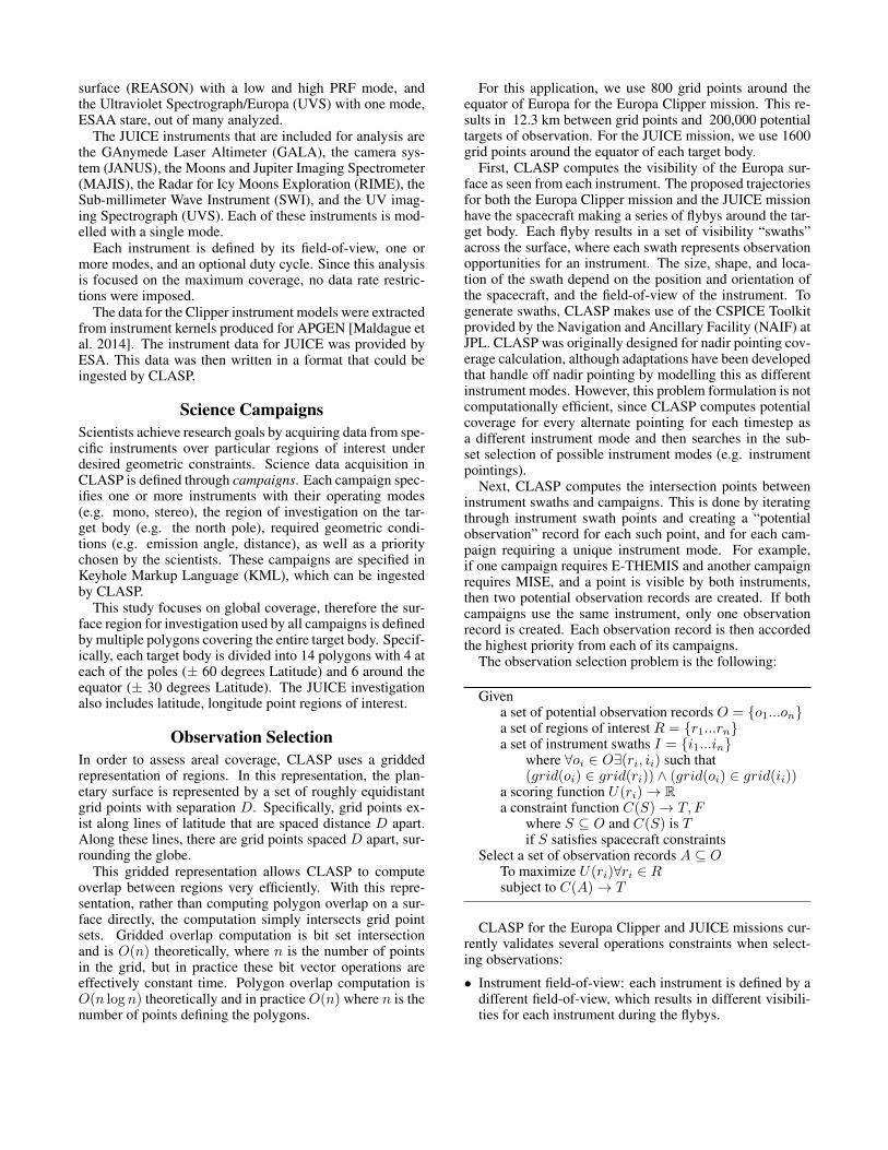
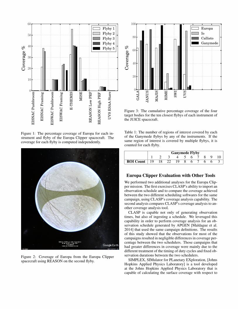
in February 2026. Each flyby was run as a separate simu-lation by changing the start time and simulation duration.A single flyby takes approximately forty minutes of wallclock time to simulate. If desired, it is possible to performpost-processing to dermine how much additional coverageis achieved by each flyby or the consequences of choosingonly a subset of flybys. Figure 1 reports the coverage re-sults for each of the instruments by flyby, where each flybycoverage is computed independently. As an example, Fig. 2shows the swath covered by REASON on the second flyby.

JUICE Coverage Analysis

CLASP was run for the JUICE campaigns and generated anobservation schedule from one squeaky wheel outer loop.Only nadir pointing was considered and all instruments wereallowed to be taking data simultaneously with no data limits.First, the coverage analysis for the JUICE mission was per-formed for the cumulative global coverage of the ten clos-est flybys for each target body: Europa, Io, Callisto, andGanymede. Like the Europa Clipper coverage analysis, eachflyby was simulated separately. These coverage results areshown in Fig. 3.

Next, at the request of ESA scientists, the coverage forregions of interest on Ganymede were determined. Each re-gion of interest is defined as a single latitude, longitude pointon the surface of Ganymede. The coverage is calculated likethe global coverage problem, but instead of having an evengrid covering the entire surface of the target body, the onlygrid points are those that make up the regions of interest.A total of 92 regions of interest were considered. Table 1summarizes the number of regions of interest that were ob-served by any instrument for each of the Ganymede flybys.If the same region of interest is seen for multiple flybys, it iscounted for each flyby.

EIS

NA

CP

ushb

room

EIS

NA

CF

ram

ing

EIS

WA

CP

ushb

room

EIS

WA

CF

ram

ing

E-T

HE

MIS

MIS

E

RE

ASO

NL

owP

RF

RE

ASO

NH

igh

PR

F

UV

SE

SAA

Star

e0

10

20

30

40

50

60C

over

age

%Flyby 1Flyby 2Flyby 3Flyby 4Flyby 5

Figure 1: The percentage coverage of Europa for each in-strument and flyby of the Europa Clipper spacecraft. Thecoverage for each flyby is computed independently.

Figure 2: Coverage of Europa from the Europa Clipperspacecraft using REASON on the second flyby.

GA

LA

JAN

US

MA

JIS

RIM

E

SWI

UV

S0

20

40

60

80

100

Cov

erag

e%

EuropaIoCallistoGanymede

Figure 3: The cumulative percentage coverage of the fourtarget bodies for the ten closest flybys of each instrument ofthe JUICE spacecraft.

Table 1: The number of regions of interest covered by eachof the Ganymede flybys by any of the instruments. If thesame region of interest is covered by multiple flybys, it iscounted for each flyby.

Ganymede Flyby1 2 3 4 5 6 7 8 9 10

ROI Count 19 18 22 19 8 6 7 6 6 3

Europa Clipper Evaluation with Other ToolsWe performed two additional analyses for the Europa Clip-per mission. The first exercises CLASP’s ability to import anobservation schedule and to compare the coverage achievedbetween the two different scheduling softwares for the samecampaign, using CLASP’s coverage analysis capability. Thesecond analysis compares CLASP’s coverage analysis to an-other coverage analysis tool.

CLASP is capable not only of generating observationtimes, but also of ingesting a schedule. We leveraged thiscapability in order to perform coverage analysis for an ob-servation schedule generated by APGEN [Maldague et al.2014] that used the same campaign definitions. The resultsof this study showed that the observations for most of thecampaigns resulted in negligible differences in coverage per-centage between the two schedulers. Those campaigns thathad greater differences in coverage were mainly due to thedifferent treatment of the timing of duty cycles and fixed ob-servation durations between the two schedulers.

SIMPLEX, SIMulator for PLanetary EXploration, [JohnsHopkins Applied Physics Laboratory] is a tool developedat the Johns Hopkins Applied Physics Laboratory that iscapable of calculating the surface coverage with respect to

science requirements. Inputs to the instrument models andscience constraints were entered into the SIMPLEX frame-work as similar as possible to those used for the CLASPcampaigns. However, the coverage calculated by SIMPLEXrevealed that the differences in modelling result in very dif-ferent coverage percentage. Particularly, the different field-of-view shapes for some of the instruments and the inabilityto specify a duty cycle created discrepencies in the coverageresults for the two different tools.

Related WorkSpacecraft operations have been a major area of applicationfor automated planning and scheduling. Numerous spacemissions have used automated planning and scheduling onthe ground to enable significant operational efficiencies in-cluding the Hubble Space Telescope [Johnston et al. 1993],space shuttle refurbishment [Deale et al. 1994], shuttle pay-load operations [Chien et al. 1999], The Modified Antarc-tic Mapping Mission [Smith, Engelhardt, and Mutz 2002],Mars Exploration Rovers [Bresina et al. 2005], Earth Ob-serving One (EO-1) [Chien et al. 2005a], Mars Express[Cesta et al. 2007; Rabenau et al. 2008], Orbital Express[Chouinard et al. 2008], and Rosetta [Chien et al. 2015].

Automated planning has even flown as a technologydemonstration on the Deep Space One (DS1) Mission[Muscettola et al. 1998] and as the primary operations sys-tem on 3CS [Chien et al. 2001], EO-1 [Chien et al. 2005b],and IPEX [Chien et al. 2016]. However, all of the above ap-plications focused on the state, resource, and timing aspectsof mission operations rather than automating both the spatialcoverage as well the state and resource reasoning.

Notable exceptions are [Knight and Hu 2009; Doubledayand Knight 2014; Rabideau et al. 2010; Doubleday 2016]which also use the CLASP system. AEOS [Lemaıtre et al.2002] also considered mapping regions but is generally fo-cused on directing an extremely agile earth observing plat-form to cover small areas from a regular earth orbit gen-erally or potentially within a single overflight. In contrastwe examine a problem with a non-agile spacecraft coveringlarge areas from a highly eccentric flyby typically in mul-tiple overflights. In [Verfaillie et al. 2012], observation re-quests are expressed in terms of time instead of geometriclocations, and the search explores the space of all possi-ble instrument start and stop times. A heuristic is used tochoose times that are expected to have the best impact onthe plan, which includes short durations to keep resource uselow. CLASP explicitly prunes times that will cause resourceviolations.

This paper is a continuation of work performed in [Ra-bideau, Chien, and Ferguson 2015], which also performedcoverage analysis for the Europa Clipper mission. However,the work in [Rabideau, Chien, and Ferguson 2015] usednotional payload instrument definitions, earlier trajectories,and focused on the comparison between choices of trajecto-ries as well as imposed data volume limits. This paper re-visited the coverage analysis of the Europa Clipper missionwith updated instruments and trajectory and also exploredcoverage analysis of the JUICE mission, which has regionsof interest.

Future WorkPossible future work for this application includes improv-ing campaign definitions and updating the state and resourcemodels to provide more accurate observation schedules thatsatisfy resource constraints and thus reflect more accuratecoverage possibilities.

Future work with respect to the CLASP software includesrepresenting articulated instruments such as in the Eagle Eyesoftware in [Knight, Donnellan, and Green 2013], which de-scribes planning and scheduling to maximize coverage bymodelling both spacecraft and instrument pointing. This isparticularly relevant to Europa Clipper as the EIS and MISEinstruments are articulated, and additionally the E-THEMISand UVS instruments can perform scans across the planetarydisk to achieve greater coverage.

Another area where this tool could be used in the futureis for mission operations, where the coverage plan could berecomputed rapidly in cases where the coverage request mixis dynamic.

ConclusionsThe work in this paper presented a tool for automatedscheduling and coverage analysis, which was used to assescoverage for the Europa Clipper and JUICE missions. Byusing geometric knowledge of the position of the spacecraft,its instruments, and a gridded representation of the observa-tion region on the target body, CLASP is able to generatea set of observable points. Then, campaign and spacecraftconstraints are applied using the Squeaky Wheel greedy op-timization algorithm. This produces possible observationschedules with the accompanying surface coverage, whichcan be used by scientists for mission analysis. A furthercomparison of the CLASP tool was performed using twodifferent tools. The first investigation used the CLASP cov-erage analysis using an observation schedule generated byAPGEN. The second comparison used the SIMPLEX toolto both generate the observation schedule and perfrom thecoverage calculation. Differences in the coverage calculatedrevealed that the scheduling algorithms and thus coverageachieved are sensitive the exact modeling of the instrumentsand cadence of the observations.

AcknowledgementsWe gratefully acknowledge the contributions of Nicolas Al-tobelli and Claire Vallat of the European Space Astron-omy Centre (ESAC)/ European Space Agency (ESA) in Vil-lanueva de la Canada, Spain, for both the JUICE relevantdata and many informative discussions.

This research was carried out at the Jet Propulsion Lab-oratory, California Institute of Technology, under a contractwith the National Aeronautics and Space Administration.

ReferencesBresina, J. L.; Jonsson, A. K.; Morris, P. H.; and Rajan, K.2005. Activity planning for the mars exploration rovers. InInternational Conference on Planning & Scheduling. Mon-terey, CA.

Cesta, A.; Cortellessa, G.; Denis, M.; Donati, A.; Fratini,S.; Oddi, A.; Policella, N.; Rabenau, E.; and Schulster, J.2007. Mexar2: AI solves mission planner problems. IEEEIntelligent Systems 22(4).Chien, S.; Rabideau, G.; Willis, J.; and Mann, T. 1999.Automating planning and scheduling of shuttle payload op-erations. Artificial Intelligence 114(1-2):239–255.Chien, S.; Engelhardt, B.; Knight, R.; Rabideau, G.; Sher-wood, R.; Hansen, E.; Ortiviz, A.; Wilklow, C.; and Wich-man, S. 2001. Onboard autonomy on the three corner satmission. In International Symposium on Artificial Intelli-gence, Robotics, and Automation in Space (i-SAIRAS 2001).Montreal, Canada.Chien, S.; Cichy, B.; Davies, A.; Tran, D.; Rabideau, G.;Castano, R.; Sherwood, R.; Mandl, D.; Frye, S.; Shulman,S.; et al. 2005a. An autonomous earth-observing sensorweb.IEEE Intelligent Systems 20(3):16–24.Chien, S.; Sherwood, R.; Tran, D.; Cichy, B.; Rabideau,G.; Castano, R.; Davis, A.; Mandl, D.; Trout, B.; Shul-man, S.; et al. 2005b. Using autonomy flight softwareto improve science return on earth observing one. Journalof Aerospace Computing, Information, and Communication2(4):196–216.Chien, S. A.; Tran, D.; Rabideau, G.; Schaffer, S. R.; Mandl,D.; and Frye, S. 2010. Timeline-based space operationsscheduling with external constraints. In International Con-ference on Planning & Scheduling. Toronto, Canada.Chien, S. A.; Rabideau, G.; Tran, D.; Troesch, M.; Double-day, J.; Nespoli, F.; Ayucar, M. P.; Sitja, M. C.; Vallat, C.;Geiger, B.; et al. 2015. Activity-based scheduling of sciencecampaigns for the rosetta orbiter. In IJCAI.Chien, S.; Doubleday, J.; Thompson, D. R.; Wagstaff, K. L.;Bellardo, J.; Francis, C.; Baumgarten, E.; Williams, A.; Yee,E.; Stanton, E.; et al. 2016. Onboard autonomy on the in-telligent payload experiment cubesat mission. Journal ofAerospace Information Systems 1–9.Chouinard, C.; Knight, R.; Jones, G.; Tran, D.; and Koblick,D. 2008. Automated and adaptive mission planning for or-bital express. In Space Operations Conference (SpaceOps2008). Heidelberg, Germany.Deale, M.; Yvanovich, M.; Schnitzuius, D.; Kautz, D.; Car-penter, M.; Zweben, M.; Davis, G.; and Daun, B. 1994. Thespace shuttle ground processing scheduling system. Intelli-gent Scheduling 423–449.Doubleday, J., and Knight, R. 2014. Science mission plan-ning for desdyni with clasp. In Space Operations Confer-ence (SpaceOps 2014). Pasadena, CA.Doubleday, J. R. 2016. Three petabytes or bust: planningscience observations for NISAR. In SPIE Asia-Pacific Re-mote Sensing. International Society for Optics and Photon-ics.European Space Agency. juice. http://sci.esa.int/juice/.Fox, B. 1996. An algorithm for scheduling improvementby schedule shifting. Technical Report 96.5.1, McDonnell

Douglas Aerospace, Houston. See also Scheduling Opti-mizer B. R. Fox US Patent 5,890,134 (1999).Google. Google Earth. https://www.google.com/earth/.Johns Hopkins Applied Physics Laboratory. SIM-PLEX SIMulator for PLanetary EXploration. http://simplex.jhuapl.edu/. Build 6.Johnston, M.; Henry, R.; Gerb, A.; Giuliano, M.; Ross, B.;Sanidas, N.; Wissler, S.; and Mainard, J. 1993. Improvingthe observing efficiency of the hubble space telescope. AIAAComputing 9.Joslin, D. E., and Clements, D. P. 1999. Squeaky wheeloptimization. Journal of Artificial Intelligence Research10:353–373.Knight, R., and Chien, S. 2006. Producing large observa-tion campaigns using compressed problem representations.In International Workshop on Planning and Scheduling forSpace (IWPSS2006). Space Telescope Science Institute,Maryland.Knight, R., and Hu, S. 2009. Compressed large-scale ac-tivity scheduling and planning (clasp) applied to desdyni.In International Workshop on Planning and Scheduling forSpace (IWPSS2009). Pasadena, California.Knight, R., and Smith, B. 2005. Optimally solving nadirobservation scheduling problems. In International Sympo-sium on Artificial Intelligence, Robotics, and Automation inSpace (i-SAIRAS 2005). Munich, Germany.Knight, R.; Donnellan, A.; and Green, J. J. 2013. Mis-sion Design Evaluation Using Automated Planning for HighResolution Imaging of Dynamic Surface Processes from theISS. In International Workshop on Planning and Schedulingfor Space (IWPSS2013). San Jose, California.Knight, R. L. 2005. Solving the constrained coverage prob-lem with flow networks as linear program approximations.Ph.D. Dissertation, University of California at Los Angeles.Lemaıtre, M.; Verfaillie, G.; Jouhaud, F.; Lachiver, J.-M.;and Bataille, N. 2002. Selecting and scheduling observa-tions of agile satellites. Aerospace Science and Technology6(5):367–381.Maldague, P. F.; Wissler, S. S.; Lenda, M. D.; and Finnerty,D. F. 2014. APGEN scheduling: 15 years of Experiencein Planning Automation. In Space Operations Conference(SpaceOps 2014). Pasadena, CA.Muscettola, N.; Nayak, P. P.; Pell, B.; and Williams, B. C.1998. Remote agent: To boldly go where no ai system hasgone before. Artificial Intelligence 103(1-2):5–47.National Aeronautics and Space Administration. EuropaClipper. https://www.nasa.gov/europa.National Aeronautics and Space Administration, NavigationAncillary Information Facility. NAIF/SPICE. https://naif.jpl.nasa.gov/naif/.Rabenau, E.; Donati, A.; Denis, M.; Policella, N.; Schul-ster, J.; Cesta, A.; Cortellessa, G.; Oddi, A.; and Fratini, S.2008. The raxem tool on mars express-uplink planning op-timisation and scheduling using ai constraint resolution. InSpaceOps 2008 Conference, 3560.

Rabideau, G.; Chien, S.; Mclaren, D.; Knight, R.; Anwar, S.;Mehall, G.; and Christensen, P. 2010. A tool for schedulingthemis observations. In International Symposium on Arti-ficial Intelligence, Robotics, and Automation for Space (i-SAIRAS 2010). European Space Agency Sapporo, Japan.Rabideau, G.; Chien, S.; and Ferguson, E. 2015. Using auto-mated scheduling for mission analysis and a case study usingthe europa clipper mission concept. In International Work-shop on Planning and Scheduling for Space (IWPSS2015).Buenos Aires, Argentina.Smith, B. D.; Engelhardt, B. E.; and Mutz, D. H. 2002. Theradarsat-mamm automated mission planner. AI Magazine23(2):25.Verfaillie, G.; Olive, X.; Pralet, C.; Rainjonneau, S.; andSebbag, I. 2012. Planning acquisitions for an ocean globalsurveillance mission. In International Symposium on Ar-tificial Intelligence, Robotics, and Automation in Space (i-SAIRAS 2012). Turin, Italy.