Using Assessed Values in Property Valuations

Dr Song ShiSchool of Economics and Finance

Massey University

Motivation

• Using assessed values to improve the sales comparison approach in property valuations– Identify valuation error sources– How to correct them– Provide new thinking and technique for real estate

appraisals

Literature

• The selection and comparison of sales can be sophisticated and complicated– Lentz and Wang (1998) classify the evolution of the

appraisal methodologies into three categories– The contemporary adjustment-grid method by Vandell

(1991), Gau, et al. (1992, 1994), and Lai, et al. (2008).– Non-traditional regression model ,artificial intelligence

and spatial analysis methods , e.g. by Peterson and Flanagan (2009), Zurada, et al. (2011), Bourassa, et al. (2010), Osland (2010) and Beamonte, et al. (2013).

What Is The Research Problem?

• However, as pointed out by Epley (1997) all these methods are“based on the presumption that a sufficient number of closed sales of comparable properties always exist in a finite time period such that a statistically reliable sample can be found…The theory is good, but not measurable or applicable (p.175-176)”.

Review of The Traditional Sales Comparison Approach

• (1)

• (2)

Where represents the ith property’s sale price at time period t1, represents the vector of land

characteristics (including lot size, shape, contour, views and other amenities), represents the

vector of building characteristics (including building age, floor area, construction materials,

condition, modernisation, number of bathrooms, garage and others), and is the

submarket/neighbourhood dummy variables.

The Proposed Approach – “The Improved Net Rate” Analysis

• Using the property’s assessed land value as a proxy to represent the land component in property valuations

• (5)– is the estimated total value of the subject property using assessed land value

statistics– is the assessed land value of the subject property– is the derived improvement value for the ith comparable property using its

assessed land value– A denotes the assessed value.

An Example of the Improved Net Rate Methodology

Comparable sales Sale 1 Sale 2 Sale 3 Sale 4 Sale 5

  Calculations of net rates

Total sale price 175,000 215,000 230,000 250,000 245,000

Less assessed land value 38,000 81,000 87,000 52,000 78,000

Improvement value 137,000 134,000 143,000 198,000 167,000

Less other improvements 10,000 15,000 15,000 18,000 14,000

Value of the dwelling 127,000 119,000 128,000 180,000 153,000

Floor area (sqm) 130 120 120 120 120

Net Rate ($psm) 977 992 1,067 1,500 1,275

Adjustments of net rates

Sales time 5.00% 3.00% 2.00% 2.00% 2.00%

Building age -3.00% 0.00% -5.00% 0.00% 0.00%

Construction materials 5.00% 0.00% 0.00% 0.00% 5.00%

Condition 0.00% 0.00% 0.00% -10.00% -15.00%

Floor area 0.00% -3.00% -3.00% -3.00% -3.00%

Modernisation/Character/Appeal 0.00% 0.00% 0.00% -10.00% -5.00%

Total adj. 7.00% 0.00% -6.00% -21.00% -16.00%

Adjusted net rate ($psm) 1,045 992 1,003 1,185 1,071

Weights on comparable sales 30% 30% 15% 10% 15%

Weighted average net rate 1,041        

Property valuation

Floor area of the subject property 130 sqm

Calculated dwelling value 135,330

Plus the assessed land value 80,000

Plus other improvements 10,000

Total current market value of property 225,330

Market value breakup

Market value of land 90,000

Market value of improvements 135,330

Current market value of property   225,330 say 225,000  

Notes: For the subject property, its assessed land value is given at $80,000; its market land value is assumed at $90,000. Other improvements value (garage, shed and fencing, etc.) is estimated at $10,000.

Estimation Errors In The Proposed Approach

• “Within” estimation error due to the proposed estimation approach– Controlled and correctable

• “Outside” estimation error due to the assessment errors in tax assessment– Non-controlled, but its impact is small when

adding more sales.

The “Within” Estimation Error

• ((β-1))/((γ*β(1+δ))/(α-(1+δ))+1), (8)

– α= , the ratio of the jth (subject) property’s assessed land value to the ith (comparable)

property’s assessed land value

– β =, the ratio of the ith (comparable) property’s assessed land value to its market land value

at time of sale

– γ= , the ratio of the ith (comparable) property’s sale price to its assessed land value at time of

sale

– δ= , building structure adjustments in percentage between the subject property and

comparable property

An Example Of Calculation α, β, γ, δ and The “Within” Estimation Error

• The “within” estimation error is calculated at 0.3%, assuming δ=15%

The “Outside” Estimation Error• Due to assessment process and methods• Assessment errors are almost unavoidable, but systematic errors such

as horizontal and vertical inequities are discouraged – Assessments must meet the minimum compliance requirements (e.g. the

IAAO (1999) standard)• Empirical test show the systematic errors are small

– Allen & Dare (2002); Cornia & Slade (2005); Goolsby (1997)– Clapp (1990); Sirmans, Diskin & Friday (1995); Cornia & Slade (2005)– Shi (2014)

• It is arguable problems of assessment errors in assessed land values are likely to be smaller than assessed values in whole, due to– The Rich GIS information for land and neighbourhoods is ready to obtain– New sophisticated techniques for land valuations (e.g. Clapp (2003), Longhofer

and Redfearn (2009), and Özdilek (2012).

Empirical Study AreaFigure 1: Suburbs and assessment boundaries for Palmerston North city

Summarised Statistics Of Dwelling Sales for Palmerston North city, March 2011 to February 2012

Total sale price ($)

Assessed total values

($)

Assessed land values

($)

Age of dwelling

(year) Floor area

(M2) Land area

(M2) Ratio of sale price to assessed land value

City

Mean 302,010 303,695 137,480 47 154 798 2.28

Maximum 1,101,500 1,375,000 780,000 >100 500 9589 5.71

Minimum 100,000 113,000 55,000 1 67 220 1.01

Std. Dev. 112,591 115,302 62,757 27 58 624 0.67

Observations 1,171 1,171 1,171 1,171 1,171 1,171 1,171

Sub 1: Hokowhitu/Aokautere Urban

Mean 388,886 400,390 207,584 44 182 737 1.98

Maximum 880,000 980,000 780,000 >100 500 2218 3.96

Minimum 175,000 190,000 85,000 1 80 312 1.01

Std. Dev. 128,332 131,526 88,204 28 64 256 0.68

Observations 191 191 191 191 191 191 191

Sub 2: Terrace End/Roslyn/Brightwater

Mean 272,758 273,064 133,340 59 138 792 2.11

Maximum 650,000 700,000 390,000 >100 345 9589 4.05

Minimum 100,000 138,000 74,000 1 67 279 1.06

Std. Dev. 90,864 90,312 54,158 24 53 752 0.53

Observations 156 156 156 156 156 156 156

Sub 3: Riverdale/Awapuni/West End/Papaeoia

Mean 287,847 289,020 150,035 68 144 725 1.92

Maximum 850,000 827,000 492,000 >100 400 2465 3.47

Minimum 110,000 160,000 80,000 10 76 220 1.01

Std. Dev. 101,200 100,801 51,573 24 54 244 0.42

Observations 254 254 254 254 254 254 254

Sub 4: Kelvin Grove/Milson/Cloverlea

Mean 313,875 310,571 111,751 27 164 698 2.75

Maximum 680,000 650,000 240,000 >100 308 2162 5.12

Minimum 143,000 170,000 72,000 1 80 383 1.56

Std. Dev. 87,483 85,054 23,299 21 54 153 0.56

Observations 289 289 289 289 289 289 289

Sub 5: Highbury/Westbrook/Takaro

Mean 236,286 237,168 111,207 48 130 726 2.11

Maximum 422,500 440,000 215,000 100 359 2082 3.35

Minimum 140,000 139,000 63,000 1 80 422 1.11

Std. Dev. 58,803 55,772 27,254 15 43 186 0.39

Observations 179 179 179 179 179 179 179 Note: Sub 1 includes valuation rolls 14700, 14660, 14670, 14710 and 14720 ; Sub 2 includes valuation rolls 14570, 14580, 14620, 14680 and 14690; Sub 3 includes valuation rolls 14480, 14730, 14550, 14560, 14600, 14610, 14650 and 14740; Sub 4 includes valuation rolls 14470, 14500, 14510 and 14590; Sub 5 includes valuation rolls 14520, 14530, 14540, 14630 and 14640. Suburb classifications are from Quotable Value New Zealand. The assessed land valuations were carried out in September 2009.

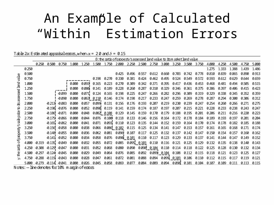
An Example of Calculated “Within” Estimation Errors

Table 2a: Estimated appraisal errors, when 𝛼= 2.0 and 𝛿 = 0.15

Notes: -- line denotes for 10% margin of errors

0.250 0.500 0.750 1.000 1.250 1.500 1.750 2.000 2.250 2.500 2.750 3.000 3.250 3.500 3.750 4.000 4.250 4.500 4.750 5.0000.250 1.275 1.333 1.388 1.439 1.4860.500 0.425 0.496 0.557 0.612 0.660 0.703 0.742 0.778 0.810 0.839 0.865 0.890 0.9130.750 0.198 0.270 0.330 0.381 0.424 0.462 0.495 0.524 0.549 0.572 0.593 0.612 0.629 0.644 0.6591.000 0.000 0.093 0.165 0.223 0.270 0.309 0.342 0.371 0.395 0.417 0.436 0.453 0.468 0.481 0.494 0.505 0.5151.250 0.000 0.080 0.141 0.189 0.228 0.260 0.287 0.310 0.329 0.346 0.361 0.375 0.386 0.397 0.406 0.415 0.4231.500 -0.099 0.000 0.071 0.124 0.165 0.198 0.225 0.247 0.266 0.282 0.296 0.309 0.319 0.329 0.338 0.345 0.352 0.3591.750 -0.090 0.000 0.063 0.110 0.146 0.174 0.198 0.217 0.233 0.247 0.259 0.269 0.278 0.287 0.294 0.300 0.306 0.3122.000 -0.213 -0.083 0.000 0.057 0.099 0.131 0.156 0.176 0.193 0.207 0.219 0.230 0.239 0.247 0.254 0.260 0.266 0.271 0.2752.250 -0.198 -0.076 0.000 0.052 0.090 0.119 0.141 0.159 0.174 0.187 0.197 0.207 0.215 0.221 0.228 0.233 0.238 0.243 0.2472.500 -0.186 -0.071 0.000 0.048 0.082 0.108 0.129 0.145 0.159 0.170 0.179 0.188 0.195 0.201 0.206 0.211 0.216 0.220 0.2232.750 -0.175 -0.066 0.000 0.044 0.076 0.100 0.118 0.133 0.146 0.156 0.164 0.172 0.178 0.184 0.189 0.193 0.197 0.201 0.2043.000 -0.165 -0.062 0.000 0.041 0.071 0.093 0.110 0.123 0.135 0.144 0.152 0.159 0.164 0.170 0.174 0.178 0.182 0.185 0.1883.250 -0.156 -0.058 0.000 0.038 0.066 0.086 0.102 0.115 0.125 0.134 0.141 0.147 0.153 0.157 0.161 0.165 0.168 0.171 0.1743.500 -0.148 -0.055 0.000 0.036 0.062 0.081 0.096 0.107 0.117 0.125 0.132 0.137 0.142 0.147 0.150 0.154 0.157 0.160 0.1623.750 -0.141 -0.052 0.000 0.034 0.058 0.076 0.090 0.101 0.110 0.117 0.123 0.129 0.133 0.137 0.141 0.144 0.147 0.149 0.1524.000 -0.319 -0.135 -0.049 0.000 0.032 0.055 0.072 0.085 0.095 0.103 0.110 0.116 0.121 0.125 0.129 0.132 0.135 0.138 0.140 0.1434.250 -0.308 -0.129 -0.047 0.000 0.031 0.052 0.068 0.080 0.090 0.098 0.104 0.110 0.114 0.118 0.122 0.125 0.128 0.130 0.132 0.1344.500 -0.297 -0.124 -0.045 0.000 0.029 0.049 0.064 0.076 0.085 0.092 0.099 0.104 0.108 0.112 0.115 0.118 0.121 0.123 0.125 0.1274.750 -0.288 -0.119 -0.043 0.000 0.028 0.047 0.061 0.072 0.081 0.088 0.094 0.099 0.103 0.106 0.110 0.112 0.115 0.117 0.119 0.1215.000 -0.279 -0.114 -0.041 0.000 0.026 0.045 0.058 0.069 0.077 0.084 0.089 0.094 0.098 0.101 0.104 0.107 0.109 0.111 0.113 0.115

β: the ratio of property's assessed land value to its market land value

γ: th

e ra

tio o

f pro

pert

y's s

ale

price

to it

s ass

esse

d la

nd v

alue

Theoretical Simulation Results of “Within” Estimation Errors

Theoretical Simulation Results Of “Outside” Estimation Errors

Empirical Simulation Results

Estimation Strategy

Comparable sales Sale 1 Sale 2 Sale 3 Sale 4 Sale 5

α 2.11 0.99 0.92 1.54 1.03

β 0.89 0.89 0.89 0.89 0.89

γ 4.61 2.65 2.64 4.81 3.14

δ 0.07 0.00 -0.06 -0.21 -0.16

Estimated valuation errors -1.93% 0.05% 0.09% -1.83% -0.73%

Land & dwelling values prior to adjustment 215,850 208,960 210,390 234,050 219,230

Land & dwelling values post to adjustment 220,096 208,852 210,196 238,411 220,843 Equally weighted average land & dwelling values 219,679

Plus other improvements values 10,000 Total property value 229,679 say 230,000

Conclusions

• The method provides a very attractive solution to the traditional sales comparison approach when comparable sales are limited.

• The impact of assessment errors is small and when more sales are added, the accuracy of valuation is improved.

• The key assumption is that neighbourhood effects are capitalised into land assessments which are uniformly assessed in an urban residential area.

• The method is easy to adopt in practice.