USING APPLIED DEMOGRAPHY IN PRODUCT DEVELOPMENT: …
32
1 USING APPLIED DEMOGRAPHY IN PRODUCT DEVELOPMENT: RESPONSE TO CHANGING MARKET CONDITIONS IN EDUCATIONAL TESTING Victoria Locke Pearson Education & University of Texas at San Antonio April 2, 2012
Transcript of USING APPLIED DEMOGRAPHY IN PRODUCT DEVELOPMENT: …

1
USING APPLIED DEMOGRAPHY IN PRODUCT DEVELOPMENT:
RESPONSE TO CHANGING MARKET CONDITIONS IN EDUCATIONAL TESTING
Victoria Locke
Pearson Education &
University of Texas at San Antonio
April 2, 2012

2
USING APPLIED DEMOGRAPHY IN PRODUCT DEVELOPMENT:
RESPONSE TO CHANGING MARKET CONDITIONS IN EDUCATIONAL TESTING
Introduction Educational reform has an impact not only on students, teachers, and schools, but also the
publishing and assessment corporations that serve the education market. As new education
reforms are enacted through Federal law, these corporations must adapt and change their
processes and procedures to remain profitable. The purpose of this research is to assist Pearson
Education adapt new sampling methodology when conducting data collection for large-scale
assessments used in schools in the United States (US). This new methodology will reduce costs
in product development while the education assessment market is changing its focus from state
assessments to national assessments.
Pearson PLC acquired Harcourt Assessment in 2008, and with it the company inherited a
line of assessment products geared towards the education market (Pearson, 2007). This market
has been in flux since accountability testing began in the 1990s. For several decades, the
standard in achievement testing in US schools was the use of norm-referenced tests such as the
Stanford series, published by Harcourt Assessment, the Iowa Tests of Basic Skills (ITBS),
published by Riverside, and the Terra-Nova, published by McGraw Hill. These assessments were
standardized using a national, representative sample of students and they provided information
on how a student ranked in areas of achievement or cognitive ability. Scores are provided that
include a Percentile Rank, Standard score, Normal Curve Equivalent or T-score. These various
scores are commonly referred to as “norms”. Within Pearson Education, the Stanford 10 is in the
product line known as Learning Assessments. This line also includes the Aprenda 3, which is an
achievement test in Spanish for children in US schools; the Naglieri NonVerbal Ability Test

3
(NNAT), the Otis-Lennon School Ability Test (OLSAT), the Orleans-Hanna Algebra Prognosis
Test, and the Stanford English or Spanish Language proficiency tests (Pearson Education, 2012)
Background
Accountability Testing, School Reform and Changing Market Conditions
Prior to the educational reform legislation known as No Child Left Behind (NCLB), norm-
referenced assessments were used to determine how children were faring cognitively and
academically in comparison with their peers. Norm-referenced tests by definition will separate
those who are doing well and able to demonstrate a high level of achievement, versus those who
are not performing as well: Half of the children will be below the 50th percentile (Rothstein,
Jacobsen, & Wilder, 2009). In particular, poor, Black and Hispanic children often scored much
lower than their Non-Hispanic White, middle-class counterparts (Kim & Sunderman, 2005). This
discrepancy is known as the achievement gap.
To hold schools, children, and districts accountable for eliminating the achievement gap
observed on norm-referenced tests, accountability assessments were implemented in several
states in the late 1980s and 1990s. Accountability took one giant leap further in 2002 with
NCLB, a reauthorization of the Elementary and Secondary Education Act (Garcia, National
Center for Research on Cultural, & Second Language Learning), commonly referred to as Title
I. NCLB mandates annual testing, and schools are held accountable for the proficiency of all
students. Schools and districts report accountability data disaggregated by race/ethnicity,
disability status, and socioeconomic status to demonstrate evidence that the gap is being reduced
(Rebell & Wolff, 2008).

4
Accountability and Impact on Learning Assessments The Stanford 10 was published the year after NCLB was enacted. After NCLB, revenue
for norm-referenced tests dropped as states turned to local standards and state-specific
proficiency testing. Product development for Learning Assessments went dormant as the
company focused on winning contracts with state departments of education to conduct their
testing. However, this assessment model also proved flawed. NCLB has been criticized for
creating a “Race to the Bottom” as states lowered standards so that more children could pass the
test (DeBray-Pelot & McGuinn, 2009). States also found that it was incredibly expensive to
create a new assessment, with unique items geared towards unique standards, year after year
(DeBray-Pelot & McGuinn, 2009).
State Consortiums Bring Market Changes
Under President Obama, the focus has changed on getting children ready for college and
careers with A Race to the Top, which encourages states to compete for money to improve
student outcomes and graduation rates through reform of the school system (U.S. Department of
Education, 2010). This change in emphasis has lead states to band together to develop a common
core curriculum. The Council of Chief State School Officers (CCSSO) and the National
Governors Association Center for Best Practices (NGA Center) produced standards in English/
language arts, history, social studies, science and mathematics that all students must achieve
upon high school graduation (Common Core State Standards Initiative, 2011). Two consortiums
of states formed to produce an assessment system, funded by the US Department of Education,
that will be based on the common core standards: The Smarter Balanced consortium, lead by the
state of Washington, and the Partnership for the Assessment of Readiness for College and
Careers (PARCC) consortium (Tamayo, 2010). Most states have aligned themselves with one or

5
both consortiums, and Pearson is now planning on updates of the norm-referenced test line of
products that will be geared towards meeting the assessment requirements of the new initiative.
The Smarter Balanced consortium is focused on being self-contained and is not planning on
using an outside vendor for assessment testing, however the PARCC consortium has opened up
the field to testing companies, including Pearson. The primary market for these assessments is
the states in the PARCC, or states that have not joined a consortium.
Prior Research Practices
Prior to 2011, when the company developed a norm-referenced test, the sample was
stratified by region, urbanicity (rural, urban, or suburban), and socioeconomic status. The regions
aligned with census regions with these differences: Maryland, Delaware, Virginia and West
Virginia were in the Northeast region, and Texas was in the West region (Pearson Education,
2003). Sample targets on these variables were created for percentages of the school age
population based on information in the decennial census. School districts were paid incentives to
participate in data collection including cash or company catalog credit.
SES Calculation
Because socioeconomic status (SES) is highly correlated with achievement (Kaushal &
Nepomnyaschy, 2009; Orfield, Frankenberg, & Lee, 2002; Tajalli & Opheim, 2005), it is a key
stratification variable to ensure the sample is representative of different levels of achievement.
Socioeconomic status was assigned at the district level, and it was derived from information
from the decennial census. A ratio was composed that took into account the percentage of the
population 18 years or older that had a high school diploma, multiplied by the median income in
the school district, and divided by 1000. This index was then divided into either thirds of the

6
distribution, used for academic tests, or fifths of the distribution, used for cognitive ability tests.
This categorical value was assigned to all schools within the district (Pearson Education, 2003).
After each school district was assigned these stratification values, districts were randomly
selected for recruiting. As school districts or schools were recruited, schools were randomly
assigned to a study: the normative study, a levels equating study (e.g., where children take on
and off grade level tests), and a forms equating study (e.g., where children take the new test, as
well as a previous edition). After the data were collected and scored, the sample was weighted to
reflect the census targets (Pearson Education, 2003).
This method worked well with samples that were large. For the Stanford 10,
approximately 500,000 children nationwide participated in the norming or equating studies
(Pearson Education, 2003). This sample size was used to ensure a wide range of performance on
the test items, which is important for norming purposes. As new forms were being developed for
the Stanford in the mid 2000s, and the sample sizes were reduced, the method did not work as
well. As sample sizes were reduced, the random district selection process yielded sample frames
that were predominately Non-Hispanic White, overwhelmingly rural, or otherwise unbalanced.
Recruiting methods grew more complicated in an effort to meet national representation, thus
increasing labor and incentive costs in data collection.
Changing Sampling Procedures to Remain Competitive
As the company responds to the common core curriculum, a major hurdle is the cost of
data collection. Using the old methods and sampling 500,000 students is not feasible in the
fluctuating market conditions. Composing a new assessment product in the very volatile
education market is risky. To save costs and mitigate the risk, the sample size for an assessment
aligned with the common core standards is 200,000 – 100,000 students. While this reduction in

7
sample size will result in reducing costs of data collection by $4 – $6 million, it presents its own
risk if the sample does not have a wide distribution of performance. Therefore, a more accurate
SES measure is needed at the school level to ensure the sample has the variability of
achievement necessary to conduct norming procedures. The goal of this research is to compose
and validate a new measure of SES at the school level that will be a more accurate predictor of
student achievement than using district-level information.
School-Level SES
Socioeconomic status is one of the most important influences in student achievement
(Orfield et al., 2002; Tajalli & Opheim, 2005). Poverty influences aspects of achievement
including absenteeism, mobility, (Tajalli & Opheim, 2005), and access to good teachers
(Darling-Hammond, 2004). Race/ethnicity, poverty, and SES are highly correlated, however in
some research student race is more important than SES as a predictor variable (Caldas &
Bankston III, 1998), other research has found that the level of poverty at a school is paramount
for predicting achievement (Aikens & Barbarin, 2008; Burros, 2008; Sanchez, Bledsoe,
Sumabat, & Ye, 2009; Southworth, 2010).
One measure commonly available to measure poverty at the school level is the
percentage of students who qualify for free or reduced price lunch (FRPL), and this percentage is
often used as a proxy variable for the socioeconomic conditions at a school (Chen-Su, 2011).
The program is administered by the U. S. Department of Agriculture, and it provides free meals
to children who live in households at or below 130% of poverty. Children who live between
130%–185% of poverty are eligible for reduced-price lunch (U.S. Department of Agriculture,
2011). In 2009, 47 percent of students were eligible for the program. The highest was in
Washington, D.C., and the lowest was in New Hampshire (Chen-Su, 2011). This measure is
8
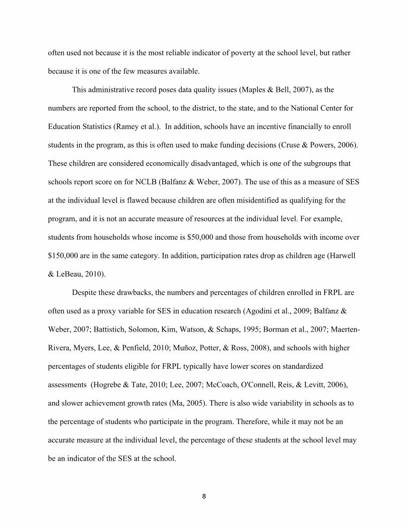
often used not because it is the most reliable indicator of poverty at the school level, but rather
because it is one of the few measures available.
This administrative record poses data quality issues (Maples & Bell, 2007), as the
numbers are reported from the school, to the district, to the state, and to the National Center for
Education Statistics (Ramey et al.). In addition, schools have an incentive financially to enroll
students in the program, as this is often used to make funding decisions (Cruse & Powers, 2006).
These children are considered economically disadvantaged, which is one of the subgroups that
schools report score on for NCLB (Balfanz & Weber, 2007). The use of this as a measure of SES
at the individual level is flawed because children are often misidentified as qualifying for the
program, and it is not an accurate measure of resources at the individual level. For example,
students from households whose income is $50,000 and those from households with income over
$150,000 are in the same category. In addition, participation rates drop as children age (Harwell
& LeBeau, 2010).
Despite these drawbacks, the numbers and percentages of children enrolled in FRPL are
often used as a proxy variable for SES in education research (Agodini et al., 2009; Balfanz &
Weber, 2007; Battistich, Solomon, Kim, Watson, & Schaps, 1995; Borman et al., 2007; Maerten-
Rivera, Myers, Lee, & Penfield, 2010; Muñoz, Potter, & Ross, 2008), and schools with higher
percentages of students eligible for FRPL typically have lower scores on standardized
assessments (Hogrebe & Tate, 2010; Lee, 2007; McCoach, O'Connell, Reis, & Levitt, 2006),
and slower achievement growth rates (Ma, 2005). There is also wide variability in schools as to
the percentage of students who participate in the program. Therefore, while it may not be an
accurate measure at the individual level, the percentage of these students at the school level may
be an indicator of the SES at the school.

9
Preliminary Analysis
To determine if the percentage of children receiving FRPL at the school would be reliable
as a proxy variable for SES, data from the 2008 – 2009 year school file were downloaded from
the Common Core of Data (CCD) available from NCES. This file had 15,983 school districts and
92,491 schools. Schools outside the 50 states were dropped from the data set, as were schools
run by the Department of Defense or the Bureau of Indian Affairs, as these schools do not
participate in field trials. Schools that had closed were dropped, as were those that were
vocational or focused only on serving a special population, such as students who are deaf or
blind.
Next, the percentage of students receiving FRPL was computed, and a univariate analysis
was run in SAS statistical software. Percentiles representing fifths of the distribution were run,
each school in the sample frame was given an SES code of 1 to 5 depending on their place in the
distribution. Upon preliminary investigation it appeared that several high poverty school
districts, including Brownsville Unified School District in Texas, had schools with a high SES
value because the number of students receiving FRPL was reported as less than 10% of the
student body. As Brownsville is in one of the poorest districts in the United States, with a child
poverty rate of 50% (U.S. Census Bureau, 2006-2008), it appeared that this measure alone would
not be an accurate means of assessing SES at the school level without identifying other areas
where the measure may be inaccurate.
To meet the research goal of having a more reliable measure of student achievement at
the school level, a more detailed process was conducted to identify the school districts that had
unreliable measures of FRPL, impute a new value for the schools in these districts, and then
assess the reliability of the measure before it is used in expensive field trials. The results are

10
reported in two sections below. The first section explains how the school-level variable was
imputed, and the second section involves its validation across state achievement tests.
Data and Methods
Composing a School level SES variable
A main challenge in this research is that there is no uniformity in how school districts are
organized across the US. Some states only have unified districts, others have unified, elementary,
and secondary school districts, resulting in some geographies overlapping. Some school districts
have sub-districts within a parent district. Some states have districts that are contiguous with
county or town boundaries, others will have multiple school districts in a single county, and
districts may overlap county lines.
The first step in the analysis was to identify districts that have a reporting error for the
percentage of students on FRPL, and the second step was to impute a value for these outlier
districts. Some indices that can be used to measure group disadvantage of an area, including
poverty, are the age and sex distribution, racial/ethnic distribution, education level of an area,
distribution of households by type, poverty ratio, child poverty, number of female headed
households, the dropout rate, proportion of housing units with 1.01 or more people per room,
median family income, and the unemployment ratio in the highest quintile (Siegel, 2002). The
percentage of people on public assistance, or welfare receipts also predict disadvantage
(McNulty & Bellair, 2003).
Data Sources
Three data sources provided information used in the analysis. The first data source was
the American Community Survey 5 year estimates 2005–2009, provided by the US Census
Bureau. The American Community Survey is a continuing monthly survey. Sampled housing

11
units receive a questionnaire, and ten to eleven million responding households are in the five
year estimates (National Research Council, 2007). The ACS 5-year estimates provide
information at the school district level. They do not provide separate information for sub-
districts. The 5 year estimates are the only estimates from the ACS that are available for small
geographic areas such as school districts (U.S. Census Bureau). For these small areas,
particularly very small school districts, the margins of error can be large.
The second data source was the Common Core Data (CCD) file from NCES as described
above, and the third data source was a list of US school districts and public schools from Market
Data Retrieval (MDR). Pearson Education subscribes to this database. MDR is owned by Dunn
and Bradstreet, and they provide databases that amalgamate information from several sources
includes NCES, Claritas, and the US Census Bureau, in addition to conducting their own surveys
of schools and school districts. The database contains information on 13,889 public school
districts, and over 116,000 total schools (Market Data Retrieval, 2010). The variables from each
data source are available in Table 1.
[Table 1 about here]
American Community Survey.
The American Community Survey 5-year estimates were downloaded from the US
Census web site to obtain demographic information at the district level, including unified,
elementary, and secondary school districts. The total number of districts from the US Census file
was 14,282 observations. Small school districts with missing data in the ACS were dropped from
analysis. Two larger school districts were missing from the file, but they were contiguous with
county boundaries; therefore, county-level information was imported from ACS and this served
as district-level information.

12
Total poverty was calculated by dividing the number of people for whom poverty status
was assessed versus the estimated population. Child poverty was calculated similarly, only
confining the ages to less than 19 years of age. The percentage of families headed by single
mothers was calculated by dividing the number of female headed families with children 18 or
under by the total number of families with children 18 or under.
Education levels in the district were calculated into four categories for adults 25 and over:
1) less than a high school education; 2) high school diploma or equivalent; 3) some college or
technical school or an Associate’s degree; 4) undergraduate degree or more. Local dropout rates
can be difficult to obtain, and are often unreliable when aggregated below the state level due to
students moving, ninth grade retention, and changes in the student population (Virginia Board of
Education, 2006). Therefore, to ascertain a more reliable proxy variable, a ratio of the number of
18 – 24 year olds in the district without a high school education was divided by the total number
of 18 – 24 year olds.
The public assistance ratio was calculated by dividing the number of households
receiving public assistance, by the total number of households. The number of rentals was the
number of rental units divided by the total number of housing units. Occupants per room was
calculated for those households with more than 1.05 per room divided by the total number of
households.
The unemployment rate was calculated as the number of people in the civilian work force
ages 20 – 69 that were unemployed, divided by the total number ages 20 – 69 in the civilian
work force. An index was calculated specifically for males aged 25–34, with the total number
not in the work force divided by the male 25–34 population.

13
The adult foreign born population was calculated for those that were foreign born divided
by the estimated population, and the percentage of adults who do not speak English was
calculated by the number of people 18+ who spoke English only divided by the total population
18+. This item was then reverse-scored.
Coefficients of variation and derived margins of error were calculated for these variables
according to procedures outlined by the US Census Bureau (U.S. Census Bureau, 2009), and
districts with derived margins of error for child poverty greater than 100 were dropped from the
data set. Most of these school districts had populations that were less than 100 total persons.
Because these variables have high multi-collinearity, a factor analysis was conducted for
data reduction. First, the data were standardized across school districts. The mean was 0 and the
standard deviation was 1 for all variables. Then a factor analysis was run with varimax rotation.
Four factors had an eigenvalue greater than 1.0. The first factor included family income and
adults 25+ with an undergraduate degree or more. These variables had factor loadings of .80 or
greater. The z-scores were added together, and this factor was named District SES. The second
factor included variables that indicate group disadvantage, including total poverty, child poverty,
public assistance, rentals, single mothers, and civilian unemployment. Each of these variables
had a factor loading of .60 or greater. The z-scores were added together, and this factor was
named District Group Disadvantage. The next factor included the variables for adults who speak
English, adults who are foreign born, and a high number of occupants per room, which is often
an indicator of large numbers of immigrants (Reitmanova & Gustafson, 2012; Yoshikawa &
Kalil, 2011). Each of these variables had a factor loading of .70 or greater. This factor was
named District Foreign Population. The last factor contained only one item, the variable for

14
adults with some college, and it was dropped from analysis. Some variables did not load on any
factor, including the proxy for dropouts, and males 25 – 34 not in the workforce.
Common Core Data and Market Data Retrieval.
Next, these data were merged with the CCD and MDR files. The MDR file was critical as
it had linking information for sub-districts and parent districts, which the CCD and ACS files did
not have. The variables downloaded from these files included the enrollment count at the school
by age, grade, race, ethnicity, and gender; number of children receiving FRPL; the school NCES
number; the NCES district number, the school operational status, sub-district status, mean
income in the zip code for the school, and the amount of money received per pupil from Title I.
Schools and districts from areas outside the fifty states, such as the Virgin Islands, Puerto Rico,
Guam, and American Samoa were deleted; Archdiocese, Military, Special Education, and
Vocational Education districts were deleted. Private, Catholic, and other parochial schools were
deleted. Charter schools were kept only if they were run by one of the school districts with
census data. If there was missing information for FRPL at the school, this school was given a
value of 0 (a new value will be imputed using the methods below), and if 5-digit zip code income
information was missing, the mean for the first 3 digits of the zip code was used. The final file
had 13,337 school districts and a total of 82,325 public schools in the fifty states.
Description of the District-Level Sample
A description of the district characteristics by region is available in Table 2. Since some
of these geographies overlap, these results cannot be inferred to accurately represent a
geographic region. Therefore, a full bivariate analysis was not conducted.
[Table 2 about here]

15
The North East had the lowest mean district percentage of students receiving FRPL at
28.95%, and the South had the highest at 59.23%. The factor for District SES was highest in the
North East (1.38), and lowest in the South (-.85). District Group Disadvantage was similarly
lowest in the North East (-1.35), and highest in the South at 1.67. The West had the highest index
for the District Foreign Population (1.95). The West also had the highest percentage of males
25 – 34 who were not in the workforce (12%) and the highest percentage of adults 18 – 24
without a High School diploma (22.6%).
Description of the School-Level Sample
Variables at the school level, available through CCD and MDR, are described in Table 3.
Since all levels of public schools were included in the analysis, and thus there are overlapping
boundaries, these results again cannot be taken to accurately describe a geographic region; they
are provided to describe the sample for the school-level imputation of an SES value. The mean
percentage of students receiving FRPL at the school level was the lowest in the North East
(31.2%) and highest in the South (56.7%). The percentage of Non-Hispanic White students was
highest in the Midwest (75.0%) and lowest in the West (46.7%). The South had the lowest
percentage of schools receiving less than $150 per student in Title 1 funds (26.2%), and the
North East had the highest percentage (57.2%). The North East had the highest median income
in the zip code at $63.8k, and the South had the lowest at $50.24k.
[Table 3 about here]
Results from OLS Regression Models
To identify outlier districts, a district mean for the percentage of the students who
qualified for FRPL was computed using OLS regression in SAS statistical software. This mean
value was then merged with the ACS variables, and it served as the outcome variable. The

16
independent variables were the District SES, District Group Disadvantage, and District Foreign
Population factors, people 18 – 24 without a high school diploma (proxy for drop outs), males
age 25 – 34 who were not in the labor force, and region, with the North East serving as the
referent group. The results are available in Table 4.
[Table 4 about here]
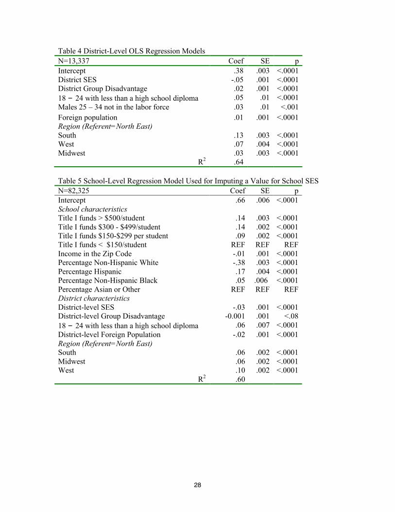
All of these variables were significant and in the expected directions. As District SES
went up, FRPL went down; similarly, as District Group Disadvantage went up, so did FRPL. As
the proxy for dropouts and males 25 – 34 not the in workforce went up, so did FRPL. The South,
Midwest, and West regions also had significantly higher district FRPL means than did the
referent region, the North East. Diagnostic graphs revealed that the regression line had the
predicted slope, and the outlier districts were easily discernible when the regression and residual
lines were plotted. The R2 was .64. All variables had a variance inflation factor less than 2.0.
All districts who had a deviance from the regression line of > .40 or < - .40 were
identified as outliers. This level was selected, as it appeared to be the point at which outlier
districts with a high index of District Group Disadvantage yet with free/reduced price lunch
status with less than 5%, were identified. This resulted in identifying 864 outlier districts, or
6.48% of the sample, with a combined total of 4,554 schools.
Next, an OLS regression was run to impute a value for FRPL at the school level for the
schools in outlier districts, or those that had a missing value. The results from the district-level
analysis were merged back into the school file. The mean of FRPL at the school was the outcome
variable, and the independent variables were: The racial/ethnic composition of the school; the
amount the school received in Title I funds; the income level in the school’s zip code; and
district level SES indicators. The results are presented in Table 5. In this model, all variables
17
were significant and in the expected direction. As the amount received in Title I funds went up,
so did the coefficient for FRPL. With the percentage of Asian or Other students serving as the
referent group, the percentage of White students was negatively significant, and the percentage
of Black students or Hispanics students was positively significant. The district level information
for SES was also significant, as was region of the country. The R2 for the school-level model was
.60. A SAS data set with the predicted values for FRPL was used to compose a school-level SAS
value. If the school was in an outlier district or had a missing value for FRPL in the CCD file,
then the predicted value of FRPL was used for school-level SES. If the school was not in an
outlier district, then the percentage of FRPL at the school was used as the school-level SES. This
variable was named school SES.
[Table 5 about here]
Validating the School SES Variable as an Indicator of Achievement Data Sources To validate that School SES was a more accurate predictor than the prior Pearson practice
of using district-level information, school-level achievement data from five states were obtained
from five state education agencies for the 2009 – 2010 academic year. The states selected for
analysis were Texas, North Carolina, New York, Missouri, and California. These states were
selected for regional representation, and the data had unrestricted access from the state education
agency. Data at the eighth grade level were selected for analysis because achievement levels tend
to dip in middle school (Shim, Ryan, & Anderson, 2008), and school lunch participation also
tends to drop during middle school (Harwell & LeBeau, 2010). Therefore the assumption was
made that if it were reliable for eighth grade, then it would be reliable for the lower grades. The
school-level achievement data were merged in with the school file with the SES indicators:
NCES FRPL, School SES, District SES, and District Group Disadvantage. Schools that were not

18
in the CCD or did not have district level information were eliminated from analysis. Separate
analyses were run for each state’s achievement tests, as they were not all on the same scale, nor
did they cover the same content as standards vary across the states. Descriptive information is
available in Table 6. New York had the most outlier schools, but this was primarily because New
York City schools did not have FRPL information in the CCD. Texas had the next highest
number of outlier schools at 10.9%. Full bivariate analyses were not conducted as the
achievement scores are all on a different scale.
Results from the OLS Regression Models
Texas.
In Texas, the mean scores for the reading/language arts (reading) and math assessment
were selected for analysis. Separate regression analyses were run with the NCES FRPL measure,
the school SES measure, and the district level information. The R2 for the NCES FRPL was .23
for reading and .19 for math. However, the School SES measure had an R2 of .52 for reading,
and .37 for math. The regression model for district level information had an R2 of .35 for reading
and .29 for math. In Texas, the school SES explained the most variance, followed by the district
level. Results are available in Table 7.
[Table 7 about here]
North Carolina.
The situation in North Carolina was somewhat different. The results in Table 8 show that
in North Carolina the R2 values for NCES FRPL were .54 for reading and .45 for math; the R2
values for the school SES were .57 for reading and .48 for math; and the model with the district
level indicators had an R2 of .14 for reading and .10 for math. Again, in North Carolina the
school SES is the most accurate predictor of school-level achievement. The difference with the

19
Texas results was that in North Carolina, the district level SES indicators were much lower than
either NCES FRPL or school SES.
[Table 8 about here]
New York.
Two separate regression analyses were run for New York, one with New York City
schools, and one without New York City schools. These were conducted separately as all New
York City schools all had a missing value for NCES FRPL, thus every school in New York City
public schools had an imputed value for school SES. In addition, without New York City, New
York state school districts are predominately small, and have very few schools. With very small
school districts, it is likely that the district-level information will be more accurate. The subject
test scores selected for analyses were English/language arts and math. The results are available in
Table 9. For the entire state, the R2 values for NCES FRPL were .02 for English/language arts
and .08 for math. Without New York City, the R2 values jumped to .64 for English/language arts
and .58 for math. The school SES also differed between these two analyses. With New York City
the R2 values were .57 for English/Language Arts and .41 for math; without New York City the
R2 values for school SES were .64 for English/language arts and .41 for math. With New York
City, district level predictors had R2 values that were .45 for English/language arts and .30 for
math; without New York City they jumped to .63 for English/language arts and .56 for math.
[Table 9 about here]
Missouri and California.
In Missouri, the subjects selected for analysis were communication arts and math. The R2
values for the NCES FRPL and school SES were the same for both of these subject areas; and
the R2 values the district level SES were less. Results are available in Table 10. In California, the

20
subjects selected were English/language arts and science. Math was not selected because the
curriculum standards changed during this school year, and it was not a reliable indicator of
school achievement. In California, the R2 values for NCES FRPL and school SES were very
similar for the two subject areas. The R2 values for district level SES were lower at .28 for
English/language arts and .29 for science. Results are available in Table 11.
[Table 10 about here]
[Table 11 about here]
Discussion
Overall, the results indicate that the percentage of students receiving free or reduced price
lunch at the school is a reliable indicator of mean student achievement at the school if the data
are scrutinized, and unrealistic or missing data are adjusted. In every state except New York
(without New York City), the new school SES was a more reliable indicator of mean student
achievement than was the district level information. These differences are especially meaningful
when a state has a larger percentage of outlier districts. Achievement in Texas was better
predicted by the school SES value, as was achievement in North Carolina. Results in that state
were especially interesting, as the district level SES appears to have very little predictive value of
student achievement. This may be because in North Carolina, school district boundaries are
mostly contiguous with either a county or city lines. In Texas, there is much more variability in
district geographical boundaries.
For sampling purposes, the next step was to divide the index for school SES into thirds of
the distribution for use in field trials for achievement products, and fifths of the distribution for
use in ability products. Univariate analyses were run separately for elementary, middle, and high

21
schools, and schools were categorized into the appropriate level of SES. This variable is
currently being piloted to determine its applicability in future data collection efforts.
Limitations and Conclusion
This research has a few limitations worthy of note. First, the state achievement data were
only analyzed for one grade level, and the assumption that the new SES variable will be valid in
other grades is being tested in the current pilot study. Second, the paucity of reliable data at the
school level to indicate SES forced the inclusion of some of the district level SES indicators to
achieve an R2 greater than .60, as some over-saturation of the model was necessary to impute a
reliable school level SES. Third, this variable is not meant to predict achievement by each
student. Within each school there will be a range of achievement, but the use of this variable will
help ensure that a wide range of achievement is obtained during data collection efforts conducted
by Pearson.

22
REFERENCES
Agodini, R., Harris, B., Atkins-Burnett, S., Heaviside, S., Novak, T., & Murphy, R. (2009). Achievement Effects of Four Early Elementary School Math Curricula: Findings from First Graders in 39 Schools. NCEE 2009-4052: National Center for Education Evaluation and Regional Assistance.
Aikens, N. L., & Barbarin, O. (2008). Socioeconomic differences in reading trajectories: The contribution of family, neighborhood, and school contexts. [Article]. Journal of Educational Psychology, 100(2), 235-251. doi: 10.1037/0022-0663.100.2.235
Balfanz, R., Legters, N., West, T.C., & Weber, L. M. (2007). Are NCLB’s measures, incentives, and improvement strategies the right ones for the nation’s low-performing High Schools? American Educational Research Journal, 44(3), 559 –593.
Battistich, V., Solomon, D., Kim, D. I., Watson, M., & Schaps, E. (1995). Schools as communities, poverty levels of student populations, and students attitudes, motives, and performance – A multilevel analysis. [Article]. American Educational Research Journal, 32(3), 627-658.
Borman, G. D., Slavin, R. E., Cheung, A. C. K., Chamberlain, A. M., Madden, N. A., & Chambers, B. (2007). Final reading outcomes of the national randomized field trial of success for all. [Article]. American Educational Research Journal, 44(3), 701-731. doi: 10.3102/0002831207306743
Burros, H. L. (2008). Change and Continuity in Grades 3-5: Effects of Poverty and Grade on Standardized Test Scores. [Article]. Teachers College Record, 110(11), 2464-2474.
Caldas, S. J., & Bankston III, C. (1998). The inequality of separation: Racial composition of schools and academic achievement. Educational Administration Quarterly, 34(4), 533-557.
Chen-Su, C. (2011). Numbers and Types of Public Elementary and Secondary Schools from the Common Core of Data: School Year 2009-2010 (NCES 2011-345). Washington, DC: U.S. Department of Education: National Center for Education Statistics.
Common Core State Standards Initiative. (2011). The Standards Retrieved April 1, 2012, from http://www.corestandards.org/about-‐the-‐standards
Cruse, C., & Powers, D. (2006). Estimating School District Poverty with Free and Reduced-Price Lunch Data. Washington, DC: U.S. Census Bureau.
Darling-Hammond, L. (2004). The color line in American education: Race, resources, and student achievement. [Electronic version]. . Du Bois Review, 1(2), 213–246.
DeBray-Pelot, E., & McGuinn, P. (2009). The New Politics of Education: Analyzing the Federal Education Policy Landscape in the Post-NCLB Era. [Article]. Educational Policy, 23(1), 15-42.

23
Garcia, E., National Center for Research on Cultural, D., & Second Language Learning, S. C. C. A. (1991). Education of Linguistically and Culturally Diverse Students: Effective Instructional Practices. Educational Practice Report: 1.
Harwell, M., & LeBeau, B. (2010). Student Eligibility for a Free Lunch as an SES Measure in Education Research. [Article]. Educational Researcher, 39(2), 120-131. doi: 10.3102/0013189x10362578
Hogrebe, M. C., & Tate, W. F. I. V. (2010). School Composition and Context Factors that Moderate and Predict 10th-Grade Science Proficiency. Teachers College Record, 112(4), 1096-1136.
Kaushal, N., & Nepomnyaschy, L. (2009). Wealth, race/ethnicity, and children's educational outcomes. [Article]. Children & Youth Services Review, 31(9), 963-971. doi: 10.1016/j.childyouth.2009.04.012
Kim, J. S., & Sunderman, G. L. (2005). Measuring Academic Proficiency Under the No Child Left Behind Act: Implications for Educational Equity. Educational Researcher, 34(8), 3–13.
Lee, J. (2007). Do national and state assessments converge for educational accountability? A meta-analytic synthesis of multiple measures in Maine and Kentucky. Applied Measurement In Education, 20(2), 171-203.
Ma, X. (2005). A Longitudinal Assessment of Early Acceleration of Students in Mathematics on Growth in Mathematics Achievement. Developmental Review, 25(1), 104-131.
Maerten-Rivera, J., Myers, N., Lee, O., & Penfield, R. (2010). Student and school predictors of high-stakes assessment in science. [Article]. Science Education, 94(6), 937-962.
Maples, J. J., & Bell, W. R. (2007). Small area estimation of school district child population and poverty: Studying use of IRS income tax data.
Market Data Retrieval. (2010). MDR Education Universe: 2010-2011. McCoach, D. B., O'Connell, A. A., Reis, S. M., & Levitt, H. A. (2006). Growing readers:
A hierarchical linear model of children's reading growth during the first 2 years of school. [Article]. Journal of Educational Psychology, 98(1), 14-28. doi: 10.1037/0022-0663.98.1.14
McNulty, T. L., & Bellair, P. E. (2003). EXPLAINING RACIAL AND ETHNIC DIFFERENCES IN ADOLESCENT VIOLENCE: STRUCTURAL DISADVANTAGE, FAMILY WELL-BEING, AND SOCIAL CAPITAL. [Article]. JQ: Justice Quarterly, 20(1), 1.
Muñoz, M. A., Potter, A. P., & Ross, S. M. (2008). Supplemental Educational Services as a Consequence of the NCLB Legislation: Evaluating its Impact on Student Achievement in a Large Urban District. [Article]. Journal of Education for Students Placed at Risk, 13(1), 1-25. doi: 10.1080/10824660701860342
National Research Council (Ed.). (2007). Using the American Community Survey: Benefits and Challenges. Washington, DC: The National Academies Press.
Orfield, G., Frankenberg, E. D., & Lee, C. (2002). The resurgence of school segregation. [Article]. Educational Leadership, 60(4), 16.
Pearson. (2007). Pearson Aquires Harcourt Assessment and Harcourt Education International from Reed Elsevier. London.

24
Pearson Education. (2003). Stanford 10: Technical Data Report. San Antonio, TX: Pearson Education.
Pearson Education. (2012). Learning Assessments Retrieved April 1, 2012, from http://www.pearsonassessments.com/pai/ea/school/schoolhome.htm
Ramey, C. T., Campbell, F. A., Burchinal, M., Skinner, M. L., Gardner, D. M., & Ramey, S. L. (2000). Persistent Effects of Early Childhood Education on High-Risk Children and Their Mothers. [Article]. Applied Developmental Science, 4(1), 2-2.
Rebell, M. A., & Wolff, J. R. (2008). Moving every child ahead: From NCLB hype to meaningful educational opportunity. New York: Teachers College Press.
Reitmanova, S., & Gustafson, D. (2012). Rethinking Immigrant Tuberculosis Control in Canada: From Medical Surveillance to Tackling Social Determinants of Health. [Review]. Journal of Immigrant and Minority Health, 14(1), 6-13. doi: 10.1007/s10903-011-9506-1
Rothstein, R., Jacobsen, R., & Wilder, T. (2009). "Proficiency for all"-an oxymoron. In M. A. Rebell & J. R. Wolff (Eds.), Reexamining the Federal effort to close the achievement gap (pp. 134-162). New York: Teachers College Press.
Sanchez, K. S., Bledsoe, L. M., Sumabat, C., & Ye, R. (2009). Hispanic students’ reading situations and problems. Journal of Hispanic Higher Education, 3(1), 50-63.
Shim, S. S., Ryan, A. M., & Anderson, C. J. (2008). Achievement goals and achievement during early adolescence: Examining time-varying predictor and outcome variables in growth-curve analysis. [Article]. Journal of Educational Psychology, 100(3), 655-671. doi: 10.1037/0022-0663.100.3.655
Siegel, J. S. (2002). Applied Demography. San Diego, CA: Academic Press. Southworth, S. (2010). Examining the Effects of School Composition on North Carolina
Student Achievement over Time. Education Policy Analysis Archives(1829). Tajalli, H., & Opheim, C. (2005). Strategies for Closing the Gap: Predicting Student
Performance in Economically Disadvantaged Schools. [Article]. Educational Research Quarterly, 28(4), 44-54.
Tamayo, J. (2010). Assessment 2.0: “Next-Generation” Comprehensive Assessment Systems: An Analysis of Proposals by the Partnership for the Assessment of Readiness for College and Careers and SMARTER Balanced Assessment Consortium: The Aspen Institute Education & Society Program.
U.S. Census Bureau. (2006-2008). American Community Survey. Accessed November 15, 2009. http://factfinder.census.gov/servlet/ADPTable?_bm=y&-‐geo_id=97000US4824990&-‐qr_name=ACS_2008_3YR_G00_DP3YR4&-‐context=adp&-‐ds_name=&-‐tree_id=3308&-‐_lang=en&-‐redoLog=false&-‐format=.
U.S. Census Bureau. (2009). A Compass for Understanding and Using American Community Survey Data: What Researchers Need to Know. Washington, DC: U.S. Census Bureau.
U.S. Department of Agriculture. (2011). Child Nutrition Programs–Income Eligibility Guidelines. edited by Food and Nutrition Service (USDA). .
U.S. Department of Education. (2010). Race to the Top Fund Retrieved April 1, 2012, from www2.ed.gov/programs/racetothetop/index.html
Virginia Board of Education. (2006). The High School Graduation Rate Formula. Richmond, VA: Virginia Board of Education.

25
Yoshikawa, H., & Kalil, A. (2011). The Effects of Parental Undocumented Status on the Developmental Contexts of Young Children in Immigrant Families. [Article]. Child Development Perspectives, 5(4), 291-297. doi: 10.1111/j.1750-8606.2011.00204.x

26
Table 1 Variables from the Data Sources American Community
Survey Common Core Data Market Data Retrieval
District Number (parent districts only)
NCES District Number (reported at sub-district level)
Sub-district status and linking information to the main district as reported in ACS
Total Population by age and sex
Percentage of race/ethnicity at the school
Income at the zip code
Total Population by sex by age, by race/ethnicity
Percentage of students receiving free or reduced price lunch
Title I funds received by the school
Own children under 18 years by Family Type and Age
Region of the country NCES Parent District Number
Family type by presence and age of related children
NCES School Number NCES School Number
Sex by age by Educational Attainment for the Population 18 years and over
Sex by age by Educational Attainment for the Population 25 years and over
Poverty Status in the Past 12 months by Sex by Age
Families Income in the past 12 months below the poverty level
Median Household Income Median Family Income Public Assistance Income for Households
Occupied Housing Units Occupancy Status Occupants per room Civilian labor force participation rates, by age, sex and race
Number of foreign born in the population, by age and sex
Language spoken by the adult population, by age and sex

27
Table 2 Descriptive Statistics – District Level of Analysis North East Midwest South West Number of districts 2,806 4,815 3,135 2,581 Free/Reduced Price Lunch 28.9% 40.3% 59.2% 49.7% District SES 1.38 -.22 -.85 -.02 District Group Disadvantage -1.35 -.87 1.67 1.16 District Foreign Population -.06 -.89 -.02 1.95 Males 25 – 34 not in the workforce 10% 9% 15% 12% 18 – 24 with less than a HS diploma 9.5% 18.1% 22.4% 22.6% Table 3 Descriptive Statistics – School level of Analysis North East Midwest South West Number of Schools 13,757 22,320 27,901 17,506 % SD % SD % SD % SD Free/Reduced price lunch 31.2 .27 43.6 .25 56.7 .25 51.9 .28 Percent White at School 65.6% 75.0% 51.5% 46.7% Percentage Hispanic at the School 14.4% 7.6% 18.6% 33.9% Percentage Black at the School 13.7% 11.7% 25.1% 4.6% Percentage Asian or Other at the School
6.3% 5.7% 4.8% 14.8%
Title I funds $500 or more per student 12.5% 11.2% 11.7% 7.7% Title I funds $300-$499 per student 10.7% 13.7% 26.2% 20.0% Title I funds $150-$299 per student 19.6% 25.1% 35.9% 29.5% Title I funds < $150 per Student, or receives no Title I
57.2% 50.0% 26.2% 42.8%
Income in the Zip Code (in thousands) 63.84 54.01 50.24 59.73
28
Table 4 District-Level OLS Regression Models N=13,337 Coef SE p Intercept .38 .003 <.0001 District SES -.05 .001 <.0001 District Group Disadvantage .02 .001 <.0001 18 – 24 with less than a high school diploma .05 .01 <.0001 Males 25 – 34 not in the labor force .03 .01 <.001 Foreign population .01 .001 <.0001 Region (Referent=North East) South .13 .003 <.0001 West .07 .004 <.0001 Midwest .03 .003 <.0001
R2 .64 Table 5 School-Level Regression Model Used for Imputing a Value for School SES N=82,325 Coef SE p Intercept .66 .006 <.0001 School characteristics Title I funds > $500/student .14 .003 <.0001 Title I funds $300 - $499/student .14 .002 <.0001 Title I funds $150-$299 per student .09 .002 <.0001 Title I funds < $150/student REF REF REF Income in the Zip Code -.01 .001 <.0001 Percentage Non-Hispanic White -.38 .003 <.0001 Percentage Hispanic .17 .004 <.0001 Percentage Non-Hispanic Black .05 .006 <.0001 Percentage Asian or Other REF REF REF District characteristics District-level SES -.03 .001 <.0001 District-level Group Disadvantage -0.001 .001 <.08 18 – 24 with less than a high school diploma .06 .007 <.0001 District-level Foreign Population -.02 .001 <.0001 Region (Referent=North East) South .06 .002 <.0001 Midwest .06 .002 <.0001 West .10 .002 <.0001
R2 .60

29
Table 6 Means, Standard Deviations, and Frequencies for Achievement Analysis in Five States
Texas North
Carolina New York
New York w/o
New York City Missouri California
Number of Schools 1,878 586 1,256 802 576 1,733 Percent of Schools That Were Outliers
10.9% < 1% 39.1% 4.6% <1% 3.6%
Outcome variables English/Language Arts / Reading Score
819.10 (28.64)
359.73 (3.76)
657.92 (13.15)
661.94 (11.24)
- 362.70 (27.19)
Communication Arts Score
- - - - 694.37 (12.76)
-
Math Score 770.77 (32.89)
362.80 (4.26)
675.39 (15.79)
677.52 (14.10)
707.44 (15.24)
-
Science Score - - - - - 384.33 (45.28)
Predictor Variables NCES FRPL .51
(.24) .56
(.20) .22
(.25) .35
(.23) .48
(.20) .57
(.28) School SES .56
(.21) .57
(.20) .43
(.22) .35
(.22) .48
(.21) .56
(.28) District SES -.35
(1.57) -.16
(1.33) .82
(1.84) .04
(2.30) -.11
(1.58) 1.46
(2.16) District Group Disadvantage
1.28 (4.02)
2.02 (2.51)
2.86 (5.55)
.05 (5.11)
1.33 (4.27)
2.62 (4.19)

30
Table 7 Texas Eighth Grade School Achievement By SES Indicators Texas Reading Math N=1878 Coef SE p Coef SE p Intercept 848.46 1.37 <.0001 801.43 1.61 <.0001 NCES FRPL -57.98 2.43 <.0001 -60.54 2.87 <.0001
R2 .23 .19 Intercept 873.96 1.29 <.0001 823.64 1.71 <.0001 School SES -97.84 2.16 <.0001 -94.30 2.85 <.0001
R2 .52 .37 Intercept 824.29 .56 <.0001 775.66 .67 <.0001 District SES 6.64 .40 <.0001 9.24 .47 <.0001 District Group Disadvantage
-2.21 .15 <.0001 -1.27 .18 <.0001
R2 .34 .29 Table 8 North Carolina Eighth Grade School Achievement By SES Indicators North Carolina Reading Math N=586 Coef SE p Coef SE p Intercept 367.36 .31 <.0001 370.76 .38 <.0001 NCES FRPL -13.53 .52 <.0001 -14.10 .64 <.0001
R2 .54 .45 Intercept 367.86 .31 <.0001 371.23 .39 <.0001 School SES -14.30 .51 <.0001 -14.83 .64 <.0001
R2 .57 .48 Intercept 360.77 .19 <.0001 363.77 .22 <.0001 District SES .24 .12 <.05 .20 .14 <.0001 District Group Disadvantage
-.50 .06 <.0001 -.46 .07 <.0001
R2 .14 .10

31
Table 9 New York Eighth Grade School Achievement By SES Indicators New York English/ Language Arts Math N=1256 Coef SE p Coef SE p Intercept 659.41 .49 <.0001 679.37 .58 <.0001 NCES FRPL -6.61 1.47 <.0001 -17.60 1.70 <.0001
R2 .02 .08 Intercept 677.23 .53 <.0001 694.96 .75 <.0001 School SES -44.55 1.09 <.0001 -45.14 1.54 <.0001
R2 .57 .41 Intercept 660.14 .37 <.0001 676.50 .51 <.0001 District SES 1.69 .16 <.0001 2.30 .08 <.0001 District Group Disadvantage
-1.26 .06 <.0001 -1.04 .08 <.0001
R2 .45 .30 New York (without New York City)
English/ Language Arts Math
N=802 Coef SE p Coef SE p Intercept 675.68 .44 <.0001 693.97 .59 <.0001 NCES FRPL -38.88 1.04 <.0001 -46.57 1.40 <.0001
R2 .64 .58 Intercept 675.83 .44 <.0001 694.14 .60 <.0001 School SES -39.99 1.07 <.0001 -47.85 1.44 <.0001
R2 .64 .41 Intercept 660.29 .27 <.0001 675.88 .37 <.0001 District SES 1.81 .13 <.0001 1.82 .17 <.0001 District Group Disadvantage
-1.15 .06 <.0001 -1.49 .08 <.0001
R2 .63 .56

32
Table 10 Missouri Eighth Grade School Achievement By SES Indicators Missouri Communication Arts Math N=577 Coef SE p Coef SE p Intercept 713.26 1.04 <.0001 731.98 1.17 <.0001 NCES FRPL -39.40 2.01 <.0001 -51.47 2.25 <.0001
R2 .40 .48 Intercept 713.22 1.04 <.0001 731.91 1.16 <.0001 School SES -39.49 2.00 <.0001 -51.29 2.24 <.0001
R2 .40 .48 Intercept 696.60 .45 <.0001 710.16 .53 <.0001 District SES .73 .32 <.05 1.21 .38 <.001 District Group Disadvantage
-1.59 .12 <.0001 -1.94 .14 <.0001
R2 .35 .39 Table 11 California Eighth Grade School Achievement By SES Indicators California English/Language Arts Science N=1732 Coef SE p Coef SE p Intercept 402.34 1.04 <.0001 444.07 1.89 <.0001 NCES FRPL -69.84 1.65 <.0001 -105.27 3.00 <.0001
R2 .51 .42 Intercept 402.49 1.05 <.0001 444.23 1.90 <.0001 School SES -70.86 1.67 <.0001 -106.65 3.04 <.0001
R2 .51 .41 Intercept 370.08 .74 <.0001 394.95 1.26 <.0001 District SES .58 .17 <.001 1.29 .30 <.0001 District Group Disadvantage
-3.14 .13 <.0001 -4.77 .23 <.0001
R2 .28 .29