Using Advanced Formulas - Cabarrus County Schools€¦ · 10 Using Advanced Formulas 170 LESSON...

170

Using Advanced Formulas10

170

LESSON SKILL MATRIX

Skills Exam Objective Objective Number

Using Formulas to Conditionally

Summarize Data

Perform logical operations by using the SUMIF function.

Perform logical operations by using the COUNTIF function.

Perform logical operations by using the AVERAGEIF function.

4.2.2

4.2.4

4.2.3

Adding Conditional Logic

Functions to Formulas

Perform logical operations by using the IF function. 4.2.1

Using Formulas to Modify Text Format text by using RIGHT, LEFT, and MID functions.

Format text by using UPPER, LOWER, and PROPER functions.

Format text by using the CONCATENATE function.

4.3.1

4.3.2

4.3.3

SOFTWARE ORIENTATION

The Formulas Tab

In this lesson, you use commands on the Formulas tab to create formulas and functions to con-ditionally summarize data, look up data, apply conditional logic, and modify text. �e Formulas tab is shown in Figure 10-1.

Create and use named ranges in formulas.

Find statistical functions such as COUNTIF, COUNTIFS, AVERAGEIF, and AVERAGEIFS here.

Math & Trig contains SUMIF and SUMIFS.

Use to create VLOOKUP and HLOOKUP functions.

Use to apply conditional logic (IF, AND, OR). Use to modify text.

Figure 10-1

The Formulas tab

�e Formulas tab contains the command groups you use to create and apply advanced formulas in Excel. Use this illustration as a reference throughout the lesson. Table 10-1 summarizes the functions covered in this lesson and speci!es where the functions are located on the Formulas tab.

Using Advanced Formulas 171

Function Category Syntax Description

SUMIF Math & Trig SUMIF(Range, Criteria,

Sum_range)

Adds the cells in Range or Sum_

range speci!ed by a given Criteria.

SUMIFS Math & Trig SUMIFS(Sum_range,

Criteria_range1, Criteria1,

Criteria_range2, Criteria2, ...)

Adds the cells in Sum_range that

meet multiple Criteria.

COUNTIF More

Functions >

Statistical

COUNTIF(Range, Criteria) Counts the number of cells within

Range that meet the Criteria.

COUNTIFS More

Functions >

Statistical

COUNTIFS(Criteria_range1,

Criteria1, Criteria_range2,

Criteria2, …)

Counts the number of cells within

multiple Criteria_range# that

meet Criteria#.

AVERAGEIF More

Functions >

Statistical

AVERAGEIF(Range, Criteria,

Average_range)

Returns the arithmetic mean of

cells in Range or Average_range

that meet a Criteria.

AVERAGEIFS More

Functions >

Statistical

AVERAGEIFS(Average_range,

Criteria_range1, Criteria1,

Criteria_range2, Criteria2, …)

Returns the mean of cells in

Average_range that meet

multiple Criteria.

VLOOKUP Lookup &

Reference

VLOOKUP(Lookup_value,

Table_array, Col_index_num,

Range_lookup)

Searches for a value in the !rst

column of Table_array and

returns a value in the same row

from Col_index_num.

HLOOKUP Lookup &

Reference

HLOOKUP(Lookup_value,

Table_array, Row_index_

num, Range_lookup)

Searches for a value in the top

row of Table_array and returns a

value in the same column from

Row_index_num.

IF Logical IF(Logical_test, Value_if_true,

Value_if_false)

When Logical_test is TRUE,

returns Value_if_true; otherwise,

it returns Value_if_false.

AND Logical AND(Logical1, Logical2, ...) Returns TRUE if all arguments are

TRUE; returns FALSE if any

argument is FALSE.

OR Logical OR(Logical1, Logical2, ...) Returns TRUE if any argument is

TRUE; returns FALSE if all

arguments are FALSE.

LEFT Text LEFT(Text, Num_chars) Returns the left Num_chars from

Text.

RIGHT Text RIGHT(Text, Num_chars) Returns the right Num_chars

from Text.

MID Text MID(Text, Start_num,

Num_chars)

Returns Num_chars from the

Text starting at Start_num.

TRIM Text TRIM(Text) Removes spaces at beginning and

end of text.

PROPER Text PROPER(Text) Capitalizes the !rst letter in each

word of text.

UPPER Text UPPER(Text) Converts text to uppercase.

LOWER Text LOWER(Text) Converts text to lowercase.

CONCATENATE Text CONCATENATE(Text1,

Text2, ...)

Joins Text1, Text2, …into a single

text string.

Table 10-1

Location and description of functions used in this lesson

Lesson 10172

USING FORMULAS TO CONDITIONALLY SUMMARIZE DATA

As you learned in Lesson 4, “Using Basic Formulas,” a formula is an equation that performs cal-culations—such as addition, subtraction, multiplication, and division—on values in a worksheet. When you enter a formula in a cell, the formula is stored internally and the results are displayed in the cell. Formulas give results and solutions that help you assess and analyze data. As you learned in Lesson 6, “Formatting Cells and Ranges,” you can use a conditional format—which changes the appearance of a cell range based on a criterion—to help you analyze data, detect critical issues, identify patterns, and visually explore trends.

Conditional formulas add yet another dimension to data analysis by summarizing data that meets one or more criteria. Criteria can be a number, text, or expression that tests which cells to sum, count, or average. A conditional formula is one in which the result is determined by the presence or absence of a particular condition. Conditional formulas used in Excel include the functions SUMIF, COUNTIF, and AVERAGEIF that check for one criterion, or their counterpoints SUM-IFS, COUNTIFS, and AVERAGEIFS that check for multiple criteria.

Using SUMIF

!e SUMIF function calculates the total of only those cells that meet a given criterion or condi-tion. !e syntax for the SUMIF function is SUMIF(Range, Criteria, Sum_range). !e values that a function uses to perform operations or calculations in a formula are called arguments. !us, the arguments of the SUMIF function are Range, Criteria, and Sum_range, which, when used together, create a conditional formula in which only those cells that meet a stated Criteria are add-ed. Cells within the Range that do not meet the criterion are not included in the total. If you use the numbers in the range for the sum, the Sum_range argument is not required. However, if you are using the criteria to test which values to sum from a di"erent column, then the range becomes the tested values and the Sum_range determines which numbers to total in the same rows as the matching criteria. In this chapter, optional arguments will be in italics.

STEP BY STEP Use the SUMIF Function

Table 10-2 explains the meaning of each argument in the SUMIF syntax. Note that if you omit Sum_range from the formula, Excel evaluates and adds the cells in the range if they match the criterion.

Argument Explanation

Range The range of cells that you want the function to evaluate. Also add the matched cells

if the Sum_range is blank.

Criteria The condition or criterion in the form of a number, expression, or text entry that

de!nes which cells will be added.

Sum_range The cells to add if the corresponding row’s cells in the Range match the criteria. If

this is blank, use the Range for both the cells to add and the cells to evaluate the

criteria against.

GET READY. LAUNCH Excel.

1. OPEN the 10 Fabrikam Sales !le for this lesson, and SAVE it to your Excel Lesson 10

folder as 10 Fabrikam Sales Solution.

2. Select H5. Click the Formulas tab and then in the Function Library group, click Math

& Trig. Scroll to and click SUMIF. The Function Arguments dialog box opens with

text boxes for the arguments, a description of the formula, and a description of each

argument.

3. In the Function Arguments dialog box, click the Collapse Dialog button for the Range

argument. This allows you to see more of the worksheet. Select the cell range C5:C16.

Press Enter. By doing this, you apply the cell range that the formula will use in the

calculation.

Table 10-2

Arguments in the SUMIF syntax


4. In the Criteria box, type >200000 and then press Tab. Figure 10-2 shows that the Sum_

range text box is not bold. This means that this argument is optional. If you leave the

Sum_range blank, Excel sums the cells you enter in the Range box. You now applied

your criteria to sum all values that are greater than $200,000.

Select cells or type range to be evaluated by the criteria. Collapse Dialog buttons

Description of current argumentRequired arguments are bold

Take Note It is not necessary to type dollar signs or commas when entering dollar amounts in the Function Arguments dialog box. If you type them, Excel removes them from the formula and returns an accurate value. �e cells in column H where you will enter formulas have already been formatted for the data.

5. Click OK to accept the changes and close the dialog box. You see that $1,657,100 of

Fabrikam’s December revenue came from properties valued in excess of $200,000.

6. If for some reason you need to edit the formula, select the cell that contains the

function, and on the Formulas tab, or in the Formula Bar, click the Insert Function

button to return to the Function Arguments dialog box (see Figure 10-3).

Insert Function buttons Excel adds quotation marks when it recognizes text or equations.

Preview of formula result

Figure 10-2

The Function Arguments dialog box guides you in building functions.

Figure 10-3

Insert Function buttons allow you to return to the Function Arguments dialog box.

Lesson 10174

Take Note �e result of the SUMIF formula in H5 does not include the property value in C15 because the formula speci�ed values greater than $200,000. To include this value, the criterion needs to be >= (greater than or equal to).

7. Click OK or press Esc if you have no changes.

8. Select cell H6, and then in the Function Library group, click Recently Used and then

click SUMIF to once again open the Function Arguments dialog box. The insertion point

should be in the Range box.

Take Note When you click Recently Used, the last function that you used appears at the top of the list. Similarly, when you click Insert Function, the Insert Function dialog box opens with the last used function highlighted.

9. In the Range !eld, select cells E5:E16. The selected range is automatically entered into

the text box. Press Tab.

Take Note You do not need to collapse the dialog box as you did in Step 3. You can directly highlight the range if the dialog box is not in the way. Another option is to move the dialog box by dragging the title bar.

10. In the Criteria box, type <3% and then press Tab. You enter the criteria to look at

column E and !nd values less than 3%.

11. In the Sum_range !eld, select cells C5:C16. The formula in H6 is different than the

formula in H5. In H6, the criteria range is different than the sum range. In H5, the

criteria range and the sum range are the same. In H6, SUMIF checks for values in

column E that are less than 3% (E8 is the !rst one) and !nds the value in the same

row and column C (C8 in this case) and adds this to the total. Click OK to accept your

changes and close the dialog box. Excel returns a value of $1,134,200.

12. SAVE the workbook.

PAUSE. LEAVE the workbook open for the next exercise.

Using SUMIFS

�e SUMIFS function adds cells in a range that meet multiple criteria. It is important to note that the order of arguments in this function is di!erent from the order used with SUMIF. In a SUMIF formula, the Sum_range argument is the third argument; in SUMIFS, however, it is the �rst argument. In this exercise, you create and use two SUMIFS formulas, each of which analyzes data based on two criteria. �e �rst SUMIFS formula adds the selling price of the properties that Fabrikam sold for more than $200,000 and that were on the market 60 days or less. �e second formula adds the properties that sold at less than 3% di!erence from their listed price within 60 days.

STEP BY STEP Use the SUMIFS Function

GET READY. USE the workbook from the previous exercise.

1. Click cell H7. On the Formulas tab, in the Function Library group, click Insert Function.

2. In the Search for a function box, type SUMIFS and then click Go. SUMIFS is highlighted

in the Select a function box.

3. Click OK to accept the function.

4. In the Function Arguments dialog box, in the Sum_range box, select cells C5:C16. This

adds your cell range to the argument of the formula.

5. In the Criteria_range1 box, select cells F5:F16. In the Criteria1 box, type <=60. This

speci!es that you want to calculate only those values that are less than or equal to 60.

When you move to the next text box, notice that Excel places quotation marks around

your criteria. It applies these marks to let itself know that this is a criterion and not a

calculated value.


6. In the Criteria_range2 box, select cells C5:C16. You are now choosing your second cell

range.

7. In the Criteria2 box, type >200000. Click OK. You now applied a second criterion that

will calculate values greater than 200,000. Excel calculates your formula, returning a

value of $742,000.

8. Select H8 and then in the Function Library group, click Recently Used.

9. Select SUMIFS. In the Sum_range box, select C5:C16.

10. In the Criteria_range1 box, select cells F5:F16. Type <=60 in the Criteria1 box.

11. In the Criteria_range2 box, select cells E5:E16. Type <3% in the Criteria2 box and then

press Tab. To see all arguments, scroll back to the top of the dialog box (see Figure

10-4).

Preview indicates total will be 433000.

Troubleshooting It is a good idea to press Tab after your last entry and preview the result of the function to make sure you entered all arguments correctly.

12. Click OK. After applying this formula, Excel returns a value of $433,000.



�e formulas you use in this exercise analyze the data on two criteria. You can continue to add up to 127 criteria on which data can be evaluated.

Because the order of arguments is di�erent in SUMIF and SUMIFS, if you want to copy and edit these similar functions, be sure to put the arguments in the correct order (�rst, second, third, and so on).

Using COUNTIF

�e COUNTIF function counts the number of cells in a given range that meet a speci�c condi-tion. �e syntax for the COUNTIF function is COUNTIF(Range, Criteria). �e Range is the

Figure 10-4

The SUMIFS function applies two or more criteria.

Lesson 10176

range of cells to be counted by the formula, and the Criteria are the conditions that must be met in order for the cells to be counted. �e condition can be a number, expression, or text entry. In this exercise, you practice using the COUNTIF function twice to calculate the number of homes sold and listed >=200,000. �e ranges you specify in these COUNTIF formulas are prices of homes. �e criterion selects only those homes that are $200,000 or more.

STEP BY STEP Use the COUNTIF Function


1. Select H9. In the Function Library group, click More Functions, select Statistical, and

then click COUNTIF.

2. In the Function Arguments dialog box, in the Range box, select cells B5:B16.

3. In the Criteria box, type >=200000 and then press Tab. Preview the result and then click

OK. You set your criteria of values greater than or equal to $200,000. Excel returns a

value of 9.

4. Select H10 and then in the Function Library group, click Recently Used.

5. Select COUNTIF. In the Functions Arguments dialog box, in the Range box, select cells

C5:C16.

6. In the Criteria box, type >=200000 and then press Tab. Preview the result and then click

OK. Excel returns a value of 7 when the formula is applied to the cell.



Using COUNTIFS

�e COUNTIFS function counts the number of cells within a range that meet multiple criteria. �e syntax is COUNTIFS(Criteria_range1, Criteria1, Criteria_range2, Criteria2, …). You can create up to 127 ranges and criteria. In this exercise, you perform calculations based on multiple criteria for the COUNTIFS formula.

STEP BY STEP Use the COUNTIFS Function


1. Select H11. In the Function Library group, click Insert Function.

2. In the Search for a function box, type COUNTIFS and then click Go. COUNTIFS is

highlighted in the Select a function box.

3. Click OK to accept the function and close the dialog box.

4. In the Function Arguments dialog box, in the Criteria_range1 box, type F5:F16. You

selected your !rst range for calculation.

5. In the Criteria1 box, type >=60 and then press Tab. The descriptions and tips for each

argument box in the Function Arguments dialog box are replaced with the value

when you move to the next argument box (see Figure 10-5). The formula result is also

displayed, enabling you to review and make corrections if an error message occurs

or an unexpected result is returned. You now set your !rst criterion. Excel shows the

calculation up to this step as a value of 8.


Preview formula result. Watch this change as each criterion is added.

6. In the Criteria_range2 box, select cells E5:E16. You selected your second range to be

calculated.

7. In the Criteria2 box, type >=5% and then press Tab to preview. Click OK. Excel returns a

value of 2.



A cell in the range you identify in the Function Arguments dialog box is counted only if all of the corresponding criteria you speci�ed are TRUE for that cell. If a criterion refers to an empty cell, COUNTIFS treats it as a 0 value.

Take Note When you create formulas, you can use the wildcard characters, question mark (?) and asterisk (*), in your criteria. A question mark matches any single character; an asterisk matches any number of characters. If you want to �nd an actual question mark or asterisk, type a grave accent ( )̀ pre-ceding the character.

Using AVERAGEIF

!e AVERAGEIF function returns the arithmetic mean of all the cells in a range that meet a given criteria. !e syntax is similar to SUMIF and is AVERAGEIF(Range, Criteria, Average_range). In the AVERAGEIF syntax, Range is the set of cells you want to average. For example, in this exer-cise, you use the AVERAGEIF function to calculate the average number of days that properties valued at $200,000 or more were on the market before they were sold. !e range in this formula is B5:B16 (cells that contain the listed value of the homes that were sold). !e criterion is the con-dition against which you want the cells to be evaluated, that is, >=200000. Average_range is the actual set of cells to average—the number of days each home was on the market before it was sold. As in the SUMIF formula, the last argument, Average_range, is optional if the range contains the cells that both match the criteria and are used for the average. In this exercise, you �rst �nd the average of all cells in a range and then �nd a conditional average.

Figure 10-5

Arguments and results for the COUNTIFS function

Lesson 10178

STEP BY STEP Use the AVERAGEIF Function


1. Select H12 and then in the Function Library group, click More Functions. Select

Statistical and then click AVERAGE.

2. In the Number1 box, type B5:B16 and then click OK. A mathematical average for this

range is returned.

3. Select H13 and then in the Function Library group, click Insert Function.

4. Select AVERAGEIF from the function list or use the function search box to locate and

accept the AVERAGEIF function. The Function Arguments dialog box opens.

5. In the Function Arguments dialog box, in the Range box, select cells B5:B16.

6. In the Criteria box, type >=200000.

7. In the Average_range box, select F5:F16 and then press Tab to preview the formula. In

the preview, Excel returns a value of 63.33.

8. Click OK to close the dialog box.



Using AVERAGEIFS

An AVERAGEIFS formula returns the average (arithmetic mean) of all cells that meet multiple criteria. �e syntax is AVERAGEIFS(Average_range, Criteria_range1, Criteria1, Criteria_range2, Criteria2, …). You learn to apply the AVERAGEIFS formula in the following exercise to !nd the average of a set of numbers where two criteria are met.

STEP BY STEP Use the AVERAGEIFS Function


1. Click cell H14. In the Function Library group, click Insert Function.

2. Type AVERAGEIFS in the Search for a function box and then click Go. AVERAGEIFS is

highlighted in the Select a function box.

3. Click OK to accept the function and close the dialog box.

4. In the Function Arguments dialog box, in the Average_range box, select cells F5:F16.

Press Tab.

5. In the Criteria_range1 box, select cells B5:B16 and then press Tab. You selected your

!rst criteria range.

6. In the Criteria1 box, type <200000. You set your !rst criteria.

7. In the Criteria_range2 box, select cells E5:E16 and then press Tab. You have selected

your second criteria range.

8. In the Criteria2 box, type <=5% and then press Tab. Click OK. Excel returns a value of

60.

9. SAVE the workbook and then CLOSE it.

PAUSE. LEAVE Excel open for the next exercise.

You entered only two criteria for the SUMIFS, COUNTIFS, and AVERAGEIFS formulas you created in the previous exercises. However, in large worksheets, you often need to use multiple cri-teria in order for the formula to return a value that is meaningful for your analysis. You can enter up to 127 conditions that data must match in order for a cell to be included in the conditional summary that results from a SUMIFS, COUNTIFS, or AVERAGEIFS formula.


�e following statements summarize how values are treated when you enter an AVERAGEIF or AVERAGEIFS formula:

• If Average_range is omitted from the function arguments, the range is used.

• If a cell in Average_range is an empty cell, AVERAGEIF ignores it.

• If the entire range is blank or contains text values, AVERAGEIF returns the #DIV/0! error value.

• If no cells in the range meet the criteria, AVERAGEIF returns the #DIV/0! error value.

USING FORMULAS TO LOOK UP DATA IN A WORKBOOK

When worksheets contain long and sometimes cumbersome lists of data, you need a way to quick-ly "nd speci"c information within these lists. �is is where Excel’s lookup functions come in handy. Lookup functions are an e$cient way to search for and insert a value in a cell when the desired value is stored elsewhere in the worksheet or even in a di%erent worksheet or workbook. VLOOKUP and HLOOKUP are the two lookup functions that you use in this section. �ese functions can return the contents of the found cell. As you work through the following exercises, note that the term table refers to a range of cells in a worksheet that can be used by a lookup function.

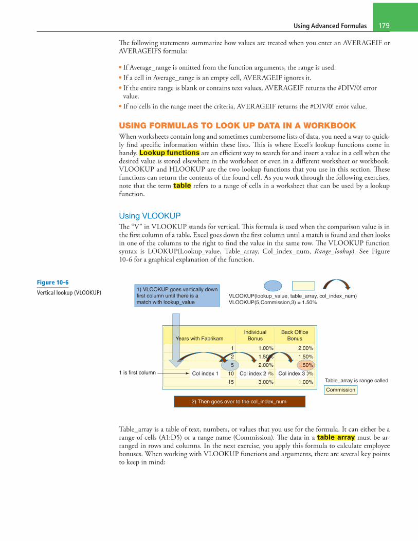
Using VLOOKUP

�e “V” in VLOOKUP stands for vertical. �is formula is used when the comparison value is in the "rst column of a table. Excel goes down the "rst column until a match is found and then looks in one of the columns to the right to "nd the value in the same row. �e VLOOKUP function syntax is LOOKUP(Lookup_value, Table_array, Col_index_num, Range_lookup). See Figure 10-6 for a graphical explanation of the function.

1

2

5

10

15

1.00%

1.50%

2.00%

2.50%

3.00%

2.00%

1.50%

1.00%

1.00%

Individual

Bonus

Back Office

Bonus

Table_array is range called

Commission

VLOOKUP(lookup_value, table_array, col_index_num)

VLOOKUP(5,Commission,3) = 1.50%

2) Then goes over to the col_index_num

1) VLOOKUP goes vertically down

first column until there is a

match with lookup_value

Col index 11 is first column Col index 2 Col index 3

1.50%

Years with Fabrikam

Table_array is a table of text, numbers, or values that you use for the formula. It can either be a range of cells (A1:D5) or a range name (Commission). �e data in a table array must be ar-ranged in rows and columns. In the next exercise, you apply this formula to calculate employee bonuses. When working with VLOOKUP functions and arguments, there are several key points to keep in mind:

Figure 10-6

Vertical lookup (VLOOKUP)

Lesson 10180

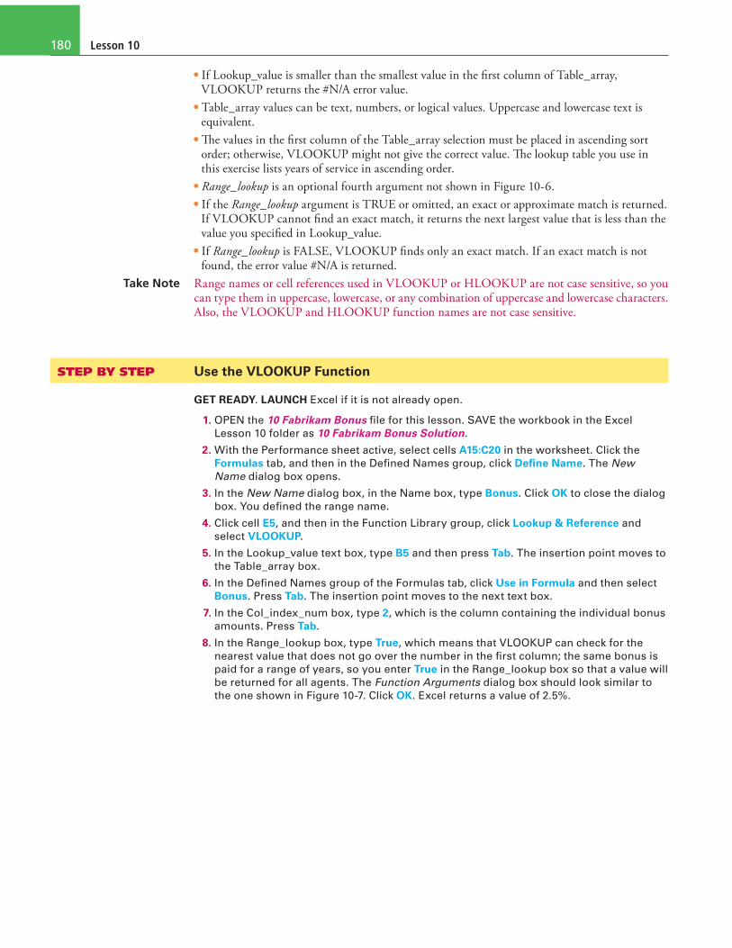
• If Lookup_value is smaller than the smallest value in the �rst column of Table_array, VLOOKUP returns the #N/A error value.

• Table_array values can be text, numbers, or logical values. Uppercase and lowercase text is equivalent.

• !e values in the �rst column of the Table_array selection must be placed in ascending sort order; otherwise, VLOOKUP might not give the correct value. !e lookup table you use in this exercise lists years of service in ascending order.

• Range_lookup is an optional fourth argument not shown in Figure 10-6.

• If the Range_lookup argument is TRUE or omitted, an exact or approximate match is returned. If VLOOKUP cannot �nd an exact match, it returns the next largest value that is less than the value you speci�ed in Lookup_value.

• If Range_lookup is FALSE, VLOOKUP �nds only an exact match. If an exact match is not found, the error value #N/A is returned.

Take Note Range names or cell references used in VLOOKUP or HLOOKUP are not case sensitive, so you can type them in uppercase, lowercase, or any combination of uppercase and lowercase characters. Also, the VLOOKUP and HLOOKUP function names are not case sensitive.

STEP BY STEP Use the VLOOKUP Function

GET READY. LAUNCH Excel if it is not already open.

1. OPEN the 10 Fabrikam Bonus !le for this lesson. SAVE the workbook in the Excel

Lesson 10 folder as 10 Fabrikam Bonus Solution.

2. With the Performance sheet active, select cells A15:C20 in the worksheet. Click the

Formulas tab, and then in the De!ned Names group, click De!ne Name. The New

Name dialog box opens.

3. In the New Name dialog box, in the Name box, type Bonus. Click OK to close the dialog

box. You de!ned the range name.

4. Click cell E5, and then in the Function Library group, click Lookup & Reference and

select VLOOKUP.

5. In the Lookup_value text box, type B5 and then press Tab. The insertion point moves to

the Table_array box.

6. In the De!ned Names group of the Formulas tab, click Use in Formula and then select

Bonus. Press Tab. The insertion point moves to the next text box.

7. In the Col_index_num box, type 2, which is the column containing the individual bonus

amounts. Press Tab.

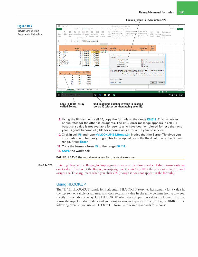
8. In the Range_lookup box, type True, which means that VLOOKUP can check for the

nearest value that does not go over the number in the !rst column; the same bonus is

paid for a range of years, so you enter True in the Range_lookup box so that a value will

be returned for all agents. The Function Arguments dialog box should look similar to

the one shown in Figure 10-7. Click OK. Excel returns a value of 2.5%.


Lookup_value is B5 (which is 12).

Look in Table_array called Bonus.

Find in column number 2; value is in same row as 10 (closest without going over 12).

9. Using the �ll handle in cell E5, copy the formula to the range E6:E11. This calculates

bonus rates for the other sales agents. The #N/A error message appears in cell E11

because a value is not available for agents who have been employed for less than one

year. (Agents become eligible for a bonus only after a full year of service.)

10. Click in cell F5 and type =VLOOKUP(B5,Bonus,3). Notice that the ScreenTip gives you

information and help as you go. This looks up values in the third column of the Bonus

range. Press Enter.

11. Copy the formula from F5 to the range F6:F11.



Take Note Entering True as the Range_lookup argument returns the closest value. False returns only an exact value. If you omit the Range_lookup argument, as in Step 10 in the previous exercise, Excel assigns the True argument when you click OK (though it does not appear in the formula).

Using HLOOKUP

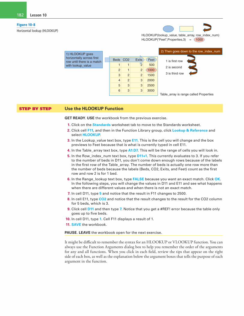
!e “H” in HLOOKUP stands for horizontal. HLOOKUP searches horizontally for a value in the top row of a table or an array and then returns a value in the same column from a row you specify in the table or array. Use HLOOKUP when the comparison values are located in a row across the top of a table of data and you want to look in a speci"ed row (see Figure 10-8). In the following exercise, you use an HLOOKUP formula to search standards for a house.

Figure 10-7

VLOOKUP Function Arguments dialog box

Lesson 10182

1 is first row

2 is second

3 is third row

Table_array is range called Properties

HLOOKUP(lookup_value, table_array, row_index_num)

HLOOKUP(“Feet”,Properties,3) = 1000

1) HLOOKUP goes

horizontally across first

row until there is a match

with lookup_value 1

2

3

4

5

6

1

1

2

2

3

3

2

2

2

3

3

3

500

Beds CO2 Exits

1500

2000

2500

3000

Feet

1000

2) Then goes down to the row_index_num

STEP BY STEP Use the HLOOKUP Function


1. Click on the Standards worksheet tab to move to the Standards worksheet.

2. Click cell F11, and then in the Function Library group, click Lookup & Reference and

select HLOOKUP.

3. In the Lookup_value text box, type E11. This is the cell you will change and the box

previews to Feet because that is what is currently typed in cell E11.

4. In the Table_array text box, type A1:D7. This will be the range of cells you will look in.

5. In the Row_index_num text box, type D11+1. This currently evaluates to 3. If you refer

to the number of beds in D11, you don’t come down enough rows because of the labels

in the !rst row of the Table_array. The number of beds is actually one row more than

the number of beds because the labels (Beds, CO2, Exits, and Feet) count as the !rst

row and row 2 is for 1 bed.

6. In the Range_lookup text box, type FALSE because you want an exact match. Click OK.

In the following steps, you will change the values in D11 and E11 and see what happens

when there are different values and when there is not an exact match.

7. In cell D11, type 5 and notice that the result in F11 changes to 2500.

8. In cell E11, type CO2 and notice that the result changes to the result for the CO2 column

for 5 beds, which is 3.

9. Click cell D11 and then type 7. Notice that you get a #REF! error because the table only

goes up to !ve beds.

10. In cell D11, type 1. Cell F11 displays a result of 1.



It might be di�cult to remember the syntax for an HLOOKUP or VLOOKUP function. You can always use the Function Arguments dialog box to help you remember the order of the arguments for any and all functions. When you click in each �eld, review the tips that appear on the right side of each box, as well as the explanation below the argument boxes that tells the purpose of each argument in the function.

Figure 10-8

Horizontal lookup (HLOOKUP)


ADDING CONDITIONAL LOGIC FUNCTIONS TO

FORMULAS

You can use the AND and OR functions to create conditional formulas that result in a logi-cal value, that is, TRUE or FALSE. Such formulas test whether a series of conditions evaluate to TRUE or FALSE. In addition, you can use the IF conditional formula that checks if a calculation evaluates as TRUE or FALSE. You can then tell IF to return one value (text, number, or logical value) if the calculation is TRUE or a di!erent value if it is FALSE.

Using IF

"e result of a conditional formula is determined by the state of a speci#c condition or the answer to a logical question. An IF function sets up a conditional statement to test data. An IF formula returns one value if the condition you specify is true and another value if it is false. "e IF function requires the following syntax: IF(Logical_test, Value_if_true, Value_if_false). In this exercise, you use an IF function to determine who achieved his goal and is eligible for the performance bonus.

STEP BY STEP Use the IF Function


1. Click the Performance worksheet tab to make it the active worksheet.

2. Click cell G5. In the Function Library group, click Logical and then click IF. The Function

Arguments dialog box opens.

3. In the Logical_test box, type D5>=C5. This component of the formula determines

whether the agent has met his or her sales goal.

4. In the Value_if_true box, type Yes. This is the value returned if the agent met his or her

goal.

5. In the Value_if_false box, type No and then click OK.

6. With G5 still selected, use the !ll handle to copy the formula to G6:G12. Excel returns

the result that three agents earned the performance award by displaying Yes in the

cells.

Take Note "e entire company is evaluated on making the goal, and bonuses are awarded to the back o$ce sta! if the company goal is met. "e result in G12 will be used for the formulas in column I. When you copy, the formatting is included.

7. Click the Auto Fill Options button in the lower-right corner of the range and choose Fill

Without Formatting. See Figure 10-9.

IF function in the Formula Bar

8. In cell H5, type =IF(G5=”Yes”,E5*D5,0. Before you complete the formula, notice the

ScreenTip, the cells selected, and the colors. Move the mouse pointer to each of the

Figure 10-9

Using the IF function

Lesson 10184

arguments and they become a hyperlink. E5 is the individual bonus rate and D5 is the

actual sales. The bonus is the rate times the sales.

9. Press Enter to complete the formula.

Take Note In some cases, Excel completes the formula. In Step 8, the closing parenthesis was not added, and Excel was able to complete the formula.

10. Click cell H5 and use the !ll handle to copy the formula to H6:H11.

11. In I5, type =IF($G$12=”Yes”,F5*D5,0) and then press Enter.

12. Use the !ll handle in I5 to copy the formula to I6:I11. Notice that Richard Carey, the

Senior Partner, did not receive an Agent Bonus and there was no bonus for Back Of!ce.

13. The !nal pending sale of $700,000 of the year came through. In D5, type $3,900,000.

Notice that H5 and the amounts in column I go from 0 to bonuses (see Figure 10-10).

G12 now displays Yes. Actual Sales now exceed the Sales Goal.



Using AND

!e AND function returns TRUE if all its arguments are true, and FALSE if one or more argu-ments are false. !e Syntax is AND(Logical1, Logical2, …). In this exercise, you use the AND function to determine whether Fabrikam’s total annual sales met the strategic goal and whether the sales goal exceeded the previous year’s sales by 5 percent.

STEP BY STEP Use the AND Function


1. Click the Annual Sales worksheet tab. Click the Formulas tab if necessary.

2. Click cell B6. In the Function Library group, click Logical and then click the AND option.

The Function Arguments dialog box opens with the insertion point in the Logical1 box.

3. Click cell B16, type >=, select cell B3, and then press Enter. This argument represents

the !rst condition: Did actual sales equal or exceed the sales goal? Because this is the

!rst year, only one logical test is entered.

4. Select cell C6, click the Recently Used button, and then click AND. In the Logical1 box,

type C16>=C3. This is the same as the condition in Step 3 (sales exceed or equals sales

goal).

Figure 10-10

Bonuses change by adding sales to D5.


5. In the Logical2 box, type C16>=B16*1.05 and then press Tab. The preview of the

formula returns TRUE, which means that both conditions in the formula have been met.

See Figure 10-11.

Result to be returned

Formula description

6. Click OK to complete the formula.

7. Select cell C6 and copy the formula to D6:F6.



Again, the AND function returns a TRUE result only when both conditions in the formula are met. For example, consider the results you achieved in the preceding exercise. Sales in the second year exceeded sales for the previous year; therefore, the �rst condition is met. Year 2 sales also exceeded Year 1 sales by 5 percent. Because both conditions are met, the formula returns a TRUE result.

Now consider the arguments for the logical tests for Year 3 (the formula in D6). Sales did not exceed the sales goal; therefore, the �rst argument returns a FALSE value. However, sales did exceed the previous year’s sales by 5 percent. When only one condition is met, the formula returns FALSE.

Using OR

Although all arguments in an AND function have to be true for the function to return a TRUE value, only one of the arguments in the OR function has to be true for the function to return a TRUE value. !e syntax for an OR function is similar to that for an AND function. With this function, the arguments must evaluate to logical values such as TRUE or FALSE or references that contain logical values. In this exercise, you create a formula that evaluates whether sales agents are eligible for the back o"ce bonus when they are new or when they did not get the sales bonus (less than 4 years with the company or did not get the agent bonus). !e OR formula returns TRUE if either of the conditions are true.

Figure 10-11

AND function arguments

Lesson 10186

STEP BY STEP Use the OR Function


1. Click on the Performance worksheet tab to activate this worksheet. Select J5 and in the

Function Library group, click Logical.

2. Click OR. The Function Arguments dialog box opens. You create a formula that answers

the following question: Has Richard Carey worked with the company for less than 4

years?

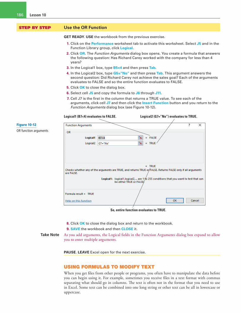
3. In the Logical1 box, type B5<4 and then press Tab.

4. In the Logical2 box, type G5=”No” and then press Tab. This argument answers the

second question: Did Richard Carey not achieve the sales goal? Each of the arguments

evaluates to FALSE and so the entire function evaluates to FALSE.

5. Click OK to close the dialog box.

6. Select cell J5 and copy the formula to J6 through J11.

7. Cell J7 is the !rst in the column that returns a TRUE value. To see each of the

arguments, click cell J7 and then click the Insert Function button and you return to the

Function Arguments dialog box (see Figure 10-12).

Logical1 (B7<4) evaluates to FALSE. Logical2 (G7=”No”) evaluates to TRUE.

So, entire function evaluates to TRUE.

8. Click OK to close the dialog box and return to the workbook.

9. SAVE the workbook and then CLOSE it.

Take Note As you add arguments, the Logical �elds in the Function Arguments dialog box expand to allow you to enter multiple arguments.


USING FORMULAS TO MODIFY TEXT

When you get �les from other people or programs, you often have to manipulate the data before you can begin using it. For example, sometimes you receive �les in a text format with commas separating what should go in columns. !e text is often not in the format that you need to use in Excel. Some text can be combined into one long string or other text can be all in lowercase or uppercase.

Figure 10-12

OR function arguments


You might be familiar with Microsoft Word’s Change Case command that enables you to change the capitalization of text. Similarly, in Excel, you can use the PROPER, UPPER, and LOWER functions to capitalize the �rst letter in each word of a text string or to convert all characters in a text string to uppercase or lowercase. �is section presents you with a text �le from the alarm company. �ere is a lot of useful information in the �le, but it is coded for the alarm system rather than for use in a spreadsheet. �e company’s president has asked you to keep the �le con�den-tial because it contains the codes for each employee, but he has also asked you to use your Excel knowledge to convert the information into a usable format.

Converting Text to Columns

You can use the Convert Text to Columns Wizard to separate simple cell content, such as �rst names and last names, into di!erent columns. Depending on how your data is organized, you can split the cell contents based on a delimiter (divider or separator), such as a space or a comma, or based on a speci�c column break location within your data. In the following exercise, you convert the data in column A to two columns.

STEP BY STEP Convert Text to Columns

GET READY. LAUNCH Excel if necessary.

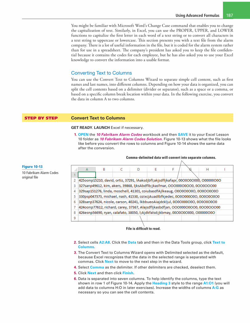
1. OPEN the 10 Fabrikam Alarm Codes workbook and then SAVE it to your Excel Lesson

10 folder as 10 Fabrikam Alarm Codes Solution. Figure 10-13 shows what the !le looks

like before you convert the rows to columns and Figure 10-14 shows the same data

after the conversion.

Comma-delimited data will convert into separate columns.

File is dif!cult to read.

2. Select cells A2:A8. Click the Data tab and then in the Data Tools group, click Text to

Columns.

3. The Convert Text to Columns Wizard opens with Delimited selected as the default,

because Excel recognizes that the data in the selected range is separated with

commas. Click Next to move to the next step in the wizard.

4. Select Comma as the delimiter. If other delimiters are checked, deselect them.

5. Click Next and then click Finish.

6. Data is separated into seven columns. To help identify the columns, type the text

shown in row 1 of Figure 10-14. Apply the Heading 3 style to the range A1:O1 (you will

add data to columns H:O in later exercises). Increase the widths of columns A:G as

necessary so you can see the cell contents.

Figure 10-13

10 Fabrikam Alarm Codes original �le

Lesson 10188

Type and format column headers. Resize columns to �t the data.



Using LEFT

�e LEFT function evaluates a string and takes any number of characters on the left side of the string. �e format of the function is LEFT(Text, Num_chars). �e !rst string in the Alarm Data workbook contains the employee’s phone extension and "oor number, which you extract by using the LEFT function.

STEP BY STEP Use the LEFT Function


1. Click cell H1, type Ext, and then in I1, type Floor to label the columns.

2. Select cell H2.

3. Click the Formulas tab. In the Function Library group, click Text and choose LEFT. The

Function Arguments dialog box opens.

4. In the Text box, click A2 and then press Tab.

5. In the Num_chars box, type 3 and then press Tab. The preview of the result shows 425.

6. Click OK and double-click on the !ll handle in the lower-right corner of cell H2 to copy

the formula in H2 to H3:H8.

7. Select cell I2, click the Recently Used button, and then select LEFT.

8. In the Text box, type A2, press Tab, and then in the Num_chars box, type 1. Click OK.

9. Copy the formula in I2 to I3:I8.



Take Note You can see the results of this and the following exercises in Figure 10-15, later in the lesson.

Using RIGHT

�e RIGHT function is almost identical to the LEFT function except that the function returns the number of characters on the right side of the text string. In the Alarm codes !le, the !rst con-verted column contains the !ve-digit employee ID at the end, and the Alarm code in column E contains the employee’s birth month.

Figure 10-14

Text is converted to columns.


STEP BY STEP Use the RIGHT Function


1. Click cell J1 and then type Birthday. In cell K1, type EmpID to label the columns.

2. Select cell J2.

3. Click the Formulas tab and then in the Function Library group, click Text and choose

RIGHT. The Function Arguments dialog box opens.

4. In the Text box, click E2 and then press Tab.

5. In the Num_chars box, type 3 and then press Tab. The preview of the result shows apr.

6. Click OK and copy the formula in J2 to J3:J8.

7. Select cell K2, type =RIGHT(A2,5), and then press Enter.

8. Copy the formula in K2 to K3:K8.



Using MID

Whereas LEFT and RIGHT return the number of the characters on either side of a text string, MID returns characters in the middle. For this reason, your arguments need to include the Text string and then a starting point (Start_num) and number of characters (Num_chars). In the �rst column of the Alarm �le, there are codes indicating two di�erent categories of employees.

STEP BY STEP Use the Mid Function


1. Click cell L1, type empcat1, and then in cell M1, type empcat2 to label the columns.

2. Select cell L2.


MID. The Function Arguments dialog box opens.

4. In the Text box, click A2 and then press Tab.

5. The starting point of the empcat1 value is the fourth character of (425oonp15210), so

type a 4 in the Start_num text box.

6. In the Num_chars box, type 2. The preview of the result shows oo.

7. Click OK and copy the formula in L2 to L3:L8.

8. Select cell M2, type =MID(A2,6,2), and then press Enter.

9. Copy the formula in M2 to M3:M8.



Using TRIM

Sometimes there are extra spaces in a cell—either at the end or the beginning of the string, es-pecially after converting a text �le like the Alarm �le—see the SPFirst and SPLast columns. !e TRIM function removes characters at both ends of the string. !ere is only one argument: Text. !us the syntax of the function is TRIM(Text).

Lesson 10190

STEP BY STEP Use the TRIM Function


1. Click cell N1, type !rst, and then in cell O1, type last to label the columns.

2. Click cell N2.


TRIM. The Function Arguments dialog box opens.

4. In the Text box, click B2. If you look closely, you see that the original value of cell B2 is

“david” with a space before the !rst name.

5. Click OK and copy the formula in N2 to N3:N8.

6. Select cell O2, type =TRIM(C2), and then press Enter.

7. Copy the formula in O2 to O3:O8.



Using PROPER

�e PROPER function capitalizes the �rst letter in a text string and any other letters in text that follow any character other than a letter. All other letters are converted to lowercase. In the PROPER(Text) syntax, Text can be text enclosed in quotation marks, a formula that returns text, or a reference to a cell containing the text you want to capitalize. In this exercise, you use PROPER to change lowercase text to initial capitals.

STEP BY STEP Use the PROPER Function


1. Click cell A11 and type First. In cell B11, type Last, and then in cell C11, type Birthday to

label the columns. Apply the Heading 3 cell style to these cells.

2. Click cell A12.


PROPER. The Function Arguments dialog box opens.

4. In the Text box, click N2. You see that david is converted to David.

5. Click OK and copy the formula in A12 to cells A12:B18 (both First and Last columns).

6. Select cell C12, type =PROPER(J2), and then press Enter.

7. Copy the formula in C12 to C13:C18.

8. SAVE the workbook and then CLOSE the !le.


Take Note �e PROPER function capitalizes the �rst letter in each word in a text string. All other letters are converted to lowercase. If you have an apostrophe within the text, such as David’s, Excel recogniz-es the apostrophe as a break and capitalizes the result as David’S.

Using UPPER

�e UPPER function allows you to convert text to uppercase (all capital letters). �e syntax is UPPER(Text), with Text referring to the text you want converted to uppercase. Text can be a ref-erence or a text string. In this exercise, you convert the employee category (empcat1 and empcat2) to uppercase.


STEP BY STEP Use the UPPER Function

GET READY. Open THE 10 Fabrikam Alarm Codes 2 WORKBOOK.

1. SAVE the workbook as 10 Fabrikam Alarm Codes Solution 2.

2. Click cell D11, type EmpCat1, and then in cell E11, type EmpCat2 to label the columns.

3. Click cell D12.


UPPER. The Function Arguments dialog box opens.

5. In the Text box, click L2. You see that oo is converted to OO.

6. Click OK and copy the formula in D12 to D12:E18 (both EmpCat1 and EmpCat2

columns).



Using LOWER

�e LOWER function converts all uppercase letters in a text string to lowercase. LOWER does not change characters in text that are not letters. You use the LOWER function in the following exercise to apply lowercase text in order to more easily tell an O (letter O) from a 0 (zero).

STEP BY STEP Use the LOWER Function


1. Click cell F11 and type oCode1. In cell G11, type oCode2 to label the columns.

2. Click cell F12.


LOWER. The Function Arguments dialog box opens.

4. In the Text box, click F2. You see that 00O0O0O000 is converted to 00o0o0o000.

5. Click OK and copy the formula in F12 from cell F12 through G18 (both oCode1 and

oCode2 columns).



Using CONCATENATE

In some cases, you need to combine text strings together. Use CONCATENATE for this pur-pose. �e syntax of the function is CONCATENATE(Text1, Text2, Text3, …). In this case, you combine the !rst and last names into two di"erent formats for future mail merges. In the !rst format, you use a comma to separate the last and !rst name but because the character can change to a semi-colon or other character, you type the comma in a cell and use the cell reference in the CONCATENATE formula.

Lesson 10192

STEP BY STEP Use the CONCATENATE Function


1. Click cell H11 and type , (a comma followed by a space). In cell I11, type First Last to

label the columns.

2. Click cell H12.


CONCATENATE. The Function Arguments dialog box opens.

4. In the Text box, click cell B12 and then press Tab. Click cell H11, press Tab, and then

click A12. In the preview area, you see “Ortiz, David.”

5. Click OK and copy the formula in cell H12 to H13:H18. The result is incorrect. Notice that

the string gets longer and longer and Ortiz is in every string.

6. Click cell H12. In the Formula Bar, click the cell H11 reference and then press F4

(Absolute). Cell H11 should become $H$11.

7. Press Enter and copy the formula in cell H12 to H13:H18 again. This time the formula is

copied correctly.

8. Select cell I12 and type =CONCATENATE(A12,” “,B12). Notice that the second argument

is a quote, space, and a quote. This separates the !rst and last names.

9. Press Enter and copy the formula in cell I12 to I13:I18.

10. Apply the Heading 3 cell style to the range D11:I11. Widen columns as necessary to

display the data. Your worksheet should be similar to Figure 10-15.


PAUSE. CLOSE the workbook and then CLOSE Excel.

Figure 10-15

The completed Fabrikam worksheet


Knowledge Assessment

Multiple Choice

Select the best response for the following statements.

1. Which of the following functions automatically counts cells that meet multiple

conditions?

a. COUNTIF

b. COUNT

c. COUNTIFS

d. SUMIFS

2. Which of the following functions automatically counts cells that meet a speci!c

condition?

a. COUNTIF

b. COUNT

c. COUNTIFS

d. SUMIFS

3. In the formula =SUMIFS(C5:C16, F5:F16, “<=60”, B5:B16, “>200000”), which of the

following is the range of cells to be added?

a. =C5:C16

b. =F5:F16

c. =B5:B16

d. =C5:F16

4. In the formula =SUMIFS(C5:C16, F5:F16,”<=60”, B5:B16, “>200000”), what does “<=60”

mean?

a. If the value in C5:C16 is greater than or equal to 60, the value in C5:C16 will be

included in the total.

b. If the value in F5:F16 is greater than or equal to 60, the value in C5:C16 will be

included in the total.

c. If the value in B5:B16 is less than or equal to 60, the value in C5:C16 will be included

in the total.

d. If the value in F5:F16 is less than or equal to 60, the value in C5:C16 will be included

in the total.

5. What does criteria range in a formula refer to?

a. The worksheet data to be included in the formula’s results

b. The range containing a condition that must be met in order for data to be included in

the result

c. The type of formula being used for the calculation

d. The type of data contained in the cells to be included in the formula

6. Which of the following functions returns one value if a condition is true and a different

value when the condition is not true?

a. AND

b. OR

c. IF

d. SUM

7. Which of the following functions returns a value if all conditions are met?

a. AND

b. OR

c. IF

d. SUM

Lesson 10194

8. Which of the following functions searches for a value in the �rst column of Table_array

and returns a value in the same row from Col_index_num?

a. AVERAGEIF

b. VLOOKUP

c. MID

d. HLOOKUP

9. Which of the following functions converts text from uppercase to title case?

a. UPPER

b. PROPER

c. LOWER

d. TRIM

10. Which of the following functions joins two or more text strings into a single text string?

a. AND

b. MID

c. TRIM

d. CONCATENATE

Projects

Project 10-1: Separating Text into Columns

In this project, you will take a text �le of student grades and separate the information into seven columns rather than one.

GET READY. LAUNCH Excel if it is not already running.

1. OPEN the 10 SFA Grades Import �le.

2. Select cells A4:A41. Click the Data tab and then in the Data Tools group, click Text to

Columns.

3. The Convert Text to Columns Wizard opens with Delimited selected as the default,

because Excel recognized that the data in the selected range is separated with

delimiters. Click Next.

4. Select Comma and Space as the delimiters. If other delimiters are checked (such as

Tab), deselect them and then click Next. Click Finish.

5. Label each of the columns in row 3 (A3 through G3): Last, First, Initial, ID, Final,

Quarter, Semester.

6. Apply the Heading 3 cell style to the column headings. Adjust the column widths to �t

the data.

7. SAVE the workbook in the Excel Lesson 10 folder as 10 SFA Grades Import Solution.

CLOSE the workbook.

LEAVE Excel open for the next project.


Project 10-2: Creating SUMIF and SUMIFS Formulas to Conditionally Summarize Data

Salary information for Contoso, Ltd. has been entered in a workbook so the o�ce manager can analyze and summarize the data. In this project, you will calculate sums with conditions.

GET READY. LAUNCH Excel if it is not already running.

1. OPEN the 10 Contoso Salaries data !le for this lesson.

2. Select cell C35. Click the Formulas tab and then in the Function Library group, click

Insert Function.

3. If the SUMIF function is not visible, type SUMIF in the Search for a function box and

then click Go. From the Select a function list, click SUMIF. Click OK.

4. In the Function Arguments dialog box, in the Range !eld select C4:C33.

5. In the Criteria box, type >100000.

6. Click OK. Because the range and sum range are the same, it is not necessary to enter a

Sum_range argument.

7. Select C36 and then click Insert Function. Select SUMIFS and then click OK.

8. In the Function Arguments dialog box, select C4:C33 as the sum range.

9. Select D4:D33 as the !rst criteria range.

10. Type >=10 as the !rst criterion.

11. Select C4:C33 as the second criteria range.

12. Type <60000 as the second criterion. Click OK to !nish the formula.

13. SAVE the workbook as 10 Contoso Salaries Solution. CLOSE the !le.

CLOSE Excel.

Using Advanced Formulas - Cabarrus County Schools€¦ · 10 Using Advanced Formulas 170 LESSON...

Documents

Transcript of Using Advanced Formulas - Cabarrus County Schools€¦ · 10 Using Advanced Formulas 170 LESSON...