Using a Hybrid Automated Valuation Model to Estimate Capital and

Eleventh Annual Pacific-Rim Real Estate Society Conference Melbourne Australia, January 23rd - 27th January, 2005

Using a Hybrid Automated Valuation Model to Estimate Capital and Site Values

Peter Rossini and Paul Kershaw Centre for Land Economics and Real Estate Research (CLEARER)

University of South Australia, Australia

Keywords: Automated Valuation Models, Property Taxation, Mass Appraisal, Residential Valuation, Hybrid Models

Abstract: In recent years the use of Hybrid Automated Valuation Models has been widely discussed in the property taxation literature. Such models are now recognised in the IAAO's standard for AVM's. These models may produce superior results to simpler AVM's and may be particularly useful in a situation where improved properties need to be used to estimate site value. Given recent court decisions in Australia that seem to require valuers to consider sales with improvements when assessing site value in "thin markets", such models may prove to be a useful tool in mass appraisal. This paper examines the use of a hybrid model to estimate capital and site values for residential properties in a small pilot study in Adelaide, South Australia. The model uses both vacant land and improved residential sales in a single model to estimate site and capital values simultaneously. This initial research shows that such models may prove to be a useful addition to the methodologies used by property tax authorities in Australia.

Introduction In recent years the use of hybrid Automated Valuation Models (AVM’s) has been widely discussed in the property taxation literature as well as in many individual reports where the results of such models are used in jurisdictions for mass appraisals. Such models are now recognised in the International Association of Assessing Officers (IAAO) standard for AVM's. These models may produce superior results to simpler AVM's and may be particularly useful in a situation where improved properties need to be used to estimate site value. Given recent court decisions in Australia that seem to require valuers to consider sales with improvements when assessing site value in "thin markets", such models may prove to be a useful tool in mass appraisal. This paper examines the use of a hybrid model to estimate capital and site values for residential properties in a small pilot study in Adelaide, South Australia. The model uses both vacant land and improved residential sales in a single model to estimate both site and capital values.

This research is partly funded through a research grant from UPmarket Software Services who provided in kind support for this research project. This research is part of a wider commercial research project to develop an automated valuation system for South Australia. This project is being developed jointing by UPmarket Software Services and the Centre for Land Economics and Real Estate Research (CLEARER) at the University of South Australia.

Rossini & Kershaw, Using a Hybrid Automated Valuation Model to Estimate Capital and Site Values

Hybrid Automated Valuation Models The IAAO standards define an automated valuation model (AVM) as

"a mathematically based computer software program that produces an estimate of market value based on market analysis of location, market conditions, and real estate characteristics from information that was previously and separately collected. The distinguishing feature of an AVM is that it is a market appraisal produced through mathematical modelling. Credibility of an AVM is dependent on the data used and the skills of the modeller producing the AVM" (IAAO, 2003 pp148)

They further recognize that these may be in an additive, multiplicative or hybrid form where the hybrid form is a

"model that incorporates both additive and multiplicative components" (IAAO, 2003 pp150)

and that these are normally hedonic models which attempt "to take observations on the overall good or service and obtain implicit prices for the goods and services. Prices are measured in terms of quantity and quality. When valuing real property, the spatial attributes and property specific attributes are valued in a single model. Calibration of the attribute components is performed statistically by regressing the overall price onto the characteristics." (IAAO, 2003 pp149)

In a study researching the valuation of land and improvements in the City of Philadelphia, McCain, Jensen et al. (2003) use some 40,000 arm’s length transactions to develop a two stage hybrid model. The first stage involved estimating a neighbourhood index for each property which was then used as input to a hybrid regression model. The neighbourhood index was estimated from the residuals of a simple hedonic model (using building and site characteristics) and then using a Kriging process to smooth out the variation. This neighbourhood variable was then used with land area, liveable area and building condition in a non-linear regression. The hybrid model was specified as (op cit)

))()(4())()()(0( 65321 bbbbb odNeighborhoLandAreabodNeighborhoConditioneaLiveableArbp +=

Where p is the price of the property.

This model is applied using both improved and unimproved sales and allows for the neighbourhood influence to be attached to both the land and improvements components at a different rate. Values for improved properties use the whole equation while vacant land estimates effectively use only the second component (since liveable area and condition are zero). This model proved to be effective even with a small set of descriptive variables. McCluskey, Deddis et al. (1998) discuss various methods of building spatial variation into mass appraisal. They discuss the problems of using submarket analysis where the submarkets often become small and the statistical analysis becomes unsound and biased (they do not discuss this in terms of non-statistical methods but the same problem applies). They then discuss the problems of using dummy variables for discrete locations such as suburbs. They point out that this "presupposes that the affect of location is uniform across all properties within a particular neighbourhood". This method also causes problems for mass appraisal authorities because of the lumpiness of assessments and broader conflicts. They suggest at more continuous approach using methods such as surface response analysis and the kriging method. These methods are applied through several of the standard GIS packages. A study of three alternative models (additive, multiplicative and non-linear) was reported by O'Connor (2002) based on work in Calgary. They used a large geographical area and used some 35,000 records randomly split into about 4/5th for model building and 1/5th for testing. They used a two level cleaning process each involving the removal of the lowest and highest 2.5% of estimate to sale ratios. They use two methods to allow for location influences; a location value response surface (LVRS) based on median prices and one based on fixed neighbourhood boundaries. Models are generated for each of the three model types and using both locational methods. The results are compared using assessment ratio statistics the



coefficient of dispersion (COD), coefficient of variation (COV) and price-related differential (PRD) as specified by the IAAO Standards on Ratio Studies (1999). They found a multiplicative model with LVRS to be superior when using both the within model and hold out data with a COV of 7 and 7.91 respectively. In a similar study involving Calgary, Gloudemans (2002, see also Gloudemans, 2002a) followed similar procedures but used more discriminating sales selection based on transaction characteristics as well as high AS ratios. They split the data into testing and model build subgroups of 5000 and 25,303 sales respectively using random selection. They then created additive (linear), multiplicative (log-linear) and Hybrid (non-linear) models. Location included in the model via a large number (hundreds) of neighbourhood dummies. The non-linear model is specified in a similar manner to that of McCain, Jensen et al. (2003) with the site and building parts being multiplicative and added together. They concluded that all three models produced good results but the multiplicative model produced the best results although they felt that it might not have produced the best results across the whole city and that the non-linear specification most closely fitted the appraisal theory.

Estimating Site and Capital Values One important advantage of these hybrid models is that they may offer a suitable solution to the valuation of land for site value purposes in situations where the number of sales is low generally called a "thin market". In the Maurici Case (High Court of Australia, February 13, 2003) summarised by Collins (2003) and applauded by Robbins (2003), the valuer was criticised for failing to consider improved properties when estimating the unimproved value and relying upon a small number of sales from a very thin market. The relative judgments in this case will not be debated in this paper but the case has re-opened the debate about using such traditional methods as the cost approach. While it is clear some of the writers on this issue have a fundamental misunderstanding of market valuation and a naive understanding of the use of cost to estimate value, the opportunity to reopen the analysis of improved sales to value vacant sites in a quantitative manner should be welcomed by academics and practitioners. One particular use of such analysis is in the derivation of site values for rating and taxation purposes. In Australia the basis for valuation for rating and taxation purposes varies from state to state. New South Wales and Queensland use unimproved value; Victorian councils have a choice of assessing capital value, net annual value or site value; Tasmania assesses capital improved value, land value and assessed annual value; Western Australia assess gross rental value, site value (urban), unimproved value (rural) and capital value (government owned properties) and South Australia asses both capital value and site value for every property. Generally site or unimproved value is used for land tax while the other bases may be used for other purposes. Site or unimproved value is assessed in all jurisdictions but is fraught with difficulties in many of the established urban (and rural) areas due to the low number of market transactions. While unimproved value is a hypothetical and non-market testable construct in most cases, its foundation is in the market for vacant rather than improved sales. If the findings of Maurici are accepted as reasonable then the scarce sales of vacant land may not be sufficient to indicate the true market value of vacant land (and therefore unimproved land) and transactions of improved properties should also be considered. Since the cost of construction rarely equals the added value of improvements (the added value tends to be either above or below the cost of construction depending on the relative supply-demand situation) this is not a suitable method for “splitting” improved sales prices into a land and building component. But this may be possible using market analysis that jointly considers the sales of both improved and vacant properties. A properly calibrated hybrid model may meet these demands. In South Australia where every property must be assessed for both capital and site value, such a hybrid model may serve the purpose of completing all valuations from a single model and lead to acceptable estimates of both site and capital value. It is with these aims in view that this research has been carried out.



Methodology Study Area This study is conducted in a small section of Metropolitan Adelaide incorporating nine suburbs. The area is located in the southern suburbs (see Appendix Figure 1) wedged between the sea to the west, hills to the east, a river and commercial district to the south and an industrial area to the north. The location contains a mixture of housing established over a 40 year period in a number of expanding developments. As a result some parts of the study area have predominantly improved sales and few vacant land sales while the newer locations have larger volumes of vacant land sales.

Study Period The study is completed using data from 1998 ands 1999. This period was chosen for three reasons. It reflects a period of time when the residential property market in the area was relatively stable and therefore no requirements for time adjustments are necessary within the models. It is also a period when the quality of data is considered to be superior. In recent years there has been a concern that some property characteristic data held by the government (and made available to industry and research groups) has become less reliable as funding for appropriate staff is reduced. This data period is more likely to have a better quality of data. Thirdly this period was used in a pervious study of Adelaide that included results for parts of this location (Rossini, 1998) and provides valuable additional information. As in previous studies the data was broken into two groups. The first group would be used to create models and the second group to test the models. This is a standard holdout sample procedure typical of most forecasting and prediction methodologies and is designed to prevent overestimating the accuracy of the models where over-fitting occurs. For this study, designation of these two data sets was based on a logical rather then random approach. If the model were to be used to assess capital and site values then the normal procedure would be to use sales from one period to estimate the values for the forthcoming assessment period. In this study we assume that the task is to create capital and site assessments in 1999 using the data from the previous year (1998) and that the assessments are then evaluated at the end of 1999 using the sales that occur during the 1999 period as the accuracy test. While this is likely to cause some “on-average” under-assessments if prices have been increasing, it does create a more realistic model and test situation.

Data For this study only detached houses and vacant land are used and allotment sizes are limited to those between 200 and 2000 sq metres. This would include the vast majority of all land uses in the study area. A large amount of data is available for each property but many of these are descriptors (such as the title reference) are not used in AVM’s and some other variables are not collected for every property. One significant set of data not available on the sales history file is a geographic midpoint for each property (which might typically be generated from a GIS). These were added to the data set from a matched file of latitudes and longitudes. The variables listed in Table 1 are suitable for the use in the AVMs and were available for every property with the building characteristics being zero in the case of vacant properties.



Table 1 - Variables used in the AVM's

Variable Variable Name/Description Sale Price SalePrice Sale Price SaleDate Longitude Easting and converted to a simple grid reference (X) Latitude Northing and converted to a simple grid reference (Y) Land Area Larea Building Area Barea Number of Main Rooms Rooms Building Condition Code Condition Building Age Bage Outer Wall cladding Converted to Dummy Variables Roof cladding Converted to Dummy Variables Building Style Converted to Dummy Variables

All relevant transactions were extracted from the sale history file and cleaned for observations with missing data or where the price was demonstrably incorrect. This was based on properties with a current A/S Ratio between .25 and 4 (the price is no more than 4 times or less than ¼ of the current assessed value). Unlike previous studies, properties that did not accurately model were not excluded. All data removed was on an a-priori basis rather the ex post approach taken by both O’Conner and Gloudemans where properties that are poorly estimated in the models are removed. That approach will tend to overestimate the accuracy of the models as some of these will be properties that are genuine transactions with correct data but that the model is incapable of properly estimating. The likely cause being omitted variables. By removing such data the opportunities to investigate these omitted variables is lost and the accuracy of the model appears better both in terms of the model statistics and the test statistics where difficult to assess properties have been removed. The approach taken in this study is to remove only those observations that are clearly incorrect or where there is missing data making it impossible to use the observations. This means that the estimates of model accuracy become quite conservative and would only be improved by diligent sales analysis and data rechecking. These would normally be carried out by a rating authority in the process of mass appraisal. As a result it is likely that a number of gross outliers will appear in the tests assessments that would not occur in a true mass appraisal. After this basic cleaning process there were 2300 observations with 47% for the model building and 53% for model testing. A break down of these observations by suburbs and land use is shown in Table 3 and by model-test and land use in Table 4.

Modelling The following is a summary of the process was used in the muti-stage modelling.

Step 1. Split the data into model and test data Step 2. Use the model data to develop linear and log-linear AVM’s using the building

and site characteristics. Select the best model and save the standardised residuals.

Step 3. Using the standardised residuals from step 2 use the latitude and longitude as and X and Y coordinate and polynomial expansions of these variables to establish a location value response surface.

Step 4. Using the surface in step 3 – estimate a new locational variable (LOCATION) for all observations. This location variable should account for major locational effects but ignore more local neighbourhood effects.



Step 5. Use the model data to develop linear, log-linear and non-linear (hybrid) models using the location, site and building characteristics. Select the best model and save the residuals.

Step 6. Using the residuals from step 2 – use a coordinate (X-Y) grid to find smoothed residual effects using a kriging approach.

Step 7. Using the “kriged” coordinate grid in step 3 – estimate a new neighbourhood variable (N-B-HOOD) for all observations. This variable should account for localised neighbourhood effects that exist in addition to the more general locational effects.

Step 8. Use the model data to develop linear, log-linear and non-linear (hybrid) models using the location, neighbourhood, site and building characteristics.

Step 9. Estimate the value for all properties using each of the three models developed at steps 5 and 8.

Step 10. Calculate accuracy statistics for model and test data and for both vacant and improved properties for each of the models in step 9. The test statistics used for this study are the mean absolute percentage error which is a standard forecast accuracy test, the mean, coefficient to variation of the assessment of sale price (A/S) ratio. These are two of the standard tests defined in the IAAO standard for ratio studies (IAAO 1999).

Results Model estimates The results of the various regression models are shown in the appendix. Models were estimated using a stepwise approach with manual manipulations to prevent multicollinearity becoming an issue. Table 5 shows the linear regression using the site and building characteristics while Table 6 shows the equivalent log-linear model. Each model uses similar variables in particular the building and land areas and building age and a number of dummy variables. In each case the variance inflation factor (VIF) indicates that there is no significant multicollinearity between any of the variables. Both models produce an R squared value of around .85 and highly significant F values. The log-linear model produces slightly superior forecasts with a higher F value and was selected as the superior model. The residuals from this model were then used in the second stage regression to estimate the locational factors using the location value response surface. The surface was estimated with an OLS estimate using a quartic order polynomial expansion of the X and Y coordinates that were derived from each properties latitude and longitude and the standardised residuals from the previous model. The results are shown as Table 7 and a graphical representation of the value surface is shown in Figure 2. The surface shows the expected responses with higher values along the coast line to the west and along the elevated hills area to the east. Values in the central area and near the industrial estate are lower with the lowest value being associated with a newer estate located near the commercial-shopping area to the south. The model shows an expected low R squared value of .217 but which is still statistically significant at greater than a 99% level of confidence. This model was used to estimate the new location variable for each property based on the properties relative position on the location value response surface. This variable was added to the data set and the models re-estimated with the inclusion of the location variable. Table 8 shows the results for the linear model and Table 9 the model for the log-linear model. In each case the model improved in its explanatory power with an increased R squared and F ratio and decreased standard error of the estimate. The log-linear model now shows clear superiority however this is to be expected since the added locational variable was estimated from the log-linear residuals at the previous step. A non-linear model was also estimated. Since the non-linear model uses a generalised least squares approach (as opposed to ordinary least squares) and this is based on an iterative



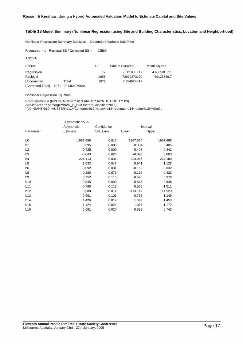
approach, it is necessary to provide starting estimates for all the model parameters (regression coefficients). These starting values were estimated from 2 preliminary regression modles firstly using vacant land sales and then using the improved sales. In each case a log-log form was used to arrive at these starting values. This followed the procedure taken by McCain, Jensen et al. (2003). The estimates for the non-linear (hybrid) model are shown in Table 10 The model is quite robust but has no better explanatory power than the linear and log-linear models. The residuals from the log-linear model were then used to estimate the neighbourhood variations using a kriging approach. The three models were then re-estimated using variables form the previous stage and the new neighbourhood variable. Results for these models are shown as linear (Table 11) log-linear (Table 12) and non-linear (Table 13). Again each model showed a statistical improvement from the previous steps with increases in R squared and F ratios and decreases in the standard errors of the estimate. Again each model showed about the same explanatory power.

Assessment estimates and accuracy While the statistical testing of models is useful, the only true test of a predictive model is to conduct out of sample testing. Table 2 shows the results for the predictive accuracy of assessments using the linear, log-linear and non-linear models with the inclusions of the locational and neighbourhood variables estimated at steps 5 and 8 and described earlier as step 9 in the methodology. The accuracy is shown separately for the improved dwellings and for the vacant properties and for the properties used within the models (1998 sales) and those held out of the model (1999 sales).

Table 2 - Accuracy tests for all models for in and out of sample data.

Absolute Percentage Errors A/S Ratio Statistics Data Model Mean

(MAPE) within 10% Average St Dev COV

Linear 9.9% 61.1% 1.016 0.128 12.631 Linear with N-Hood 9.7% 66.1% 1.008 0.124 12.291 Log-Linear 9.6% 61.1% 1.041 0.126 12.072 Log-Linear with N-Hood 6.8% 83.7% 1.071 0.129 12.042 Hybrid 9.7% 64.8% 1.031 0.111 10.734

Dwellings Model Data (1998)

Hybrid with N-Hood 7.4% 79.4% 1.033 0.110 10.622 Linear 10.6% 54.2% 0.967 0.127 13.151 Linear with N-Hood 11.6% 50.6% 0.957 0.125 13.054 Log-Linear 10.6% 54.6% 0.985 0.126 12.781 Log-Linear with N-Hood 10.0% 56.6% 1.027 0.145 14.143 Hybrid 9.6% 61.4% 0.986 0.125 12.694

Dwellings Test Data (1999)


Vacant Model Data (1998)


Vacant Test Data (1999)

Hybrid with N-Hood 13.5% 49.4% 0.968 0.294 30.331



Improved properties The results for the improved dwellings shows that the models including the neighbourhood variable were significantly better for the log-linear and hybrid models when considering the in sample data but when using the holdout or test data, these models did not perform better. This suggests that that the use of the neighbourhood variable based on the kriging of the residuals does not improve the predictive accuracy of the models and that the original model is over-fitted. The out of sample tests for dwellings show that the hybrid model does produce superior assessment although the addition of the neighbourhood variables does not improve the model. The accuracy of these assessments is comparable to current assessed values in South Australia. In his paper discussing the accuracy requirements of automated and intelligent systems, Rossini (1999) analyses the accuracy of assessed values for detached dwellings over the whole Adelaide metropolitan area for sales within a 3 month period in 1998. He found the mean error of -8.48% suggesting a systematic underestimation of values with a MAPE of 11.47% and only 50.8% of values being within a 10% margin of errors. After correcting for the systematic underestimation (which has not been carried out in this study) the results showed an MAPE of 9.53% with 62.5% of values being with the 10% margin for error. This is consistent with the results from the hybrid model. This is impressive when considering that these estimates are based on a single model and where sales circumstances and the physical data have not been validated. Typical sales analysis and data validation would significantly improve these results.

Vacant Properties The results for the vacant land models are less accurate. The estimates for the properties within the model are less accurate than those for the improved properties with the basic linear and hybrid models (without the neighbour hood) producing the best and similar results. The accuracy of the predictions for the out of sample hold out properties are considerably worse than for the improved properties. Some of this is due to the higher levels of growth in vacant land prices. While the A/S ratios are just below 1 for the improved test data suggesting that prices may have risen by around 2 %, the A/S ratios for the vacant land test data are considerably less than 1 for all models and would suggest that prices had risen by about 4 to 6 percent. This would explain the higher MAPE and lower numbers of estimates within 10% however it does not explain why the standard deviation and hence the COV are so much greater. These results are probably what we would expect given that we have only one property descriptor (land area) as well as the wider location variables. There are also less observations and many of the estimates will be based on locations where there are very few sales. While these errors cast some doubt on the suitability of using such a mode for site value estimates (the calculation can be applied to the improved properties to estimate site value as well) these values are at least highly consistent and could be defended as using all available sales in the location. Broader locational influences are estimated better through the use of the improved sales as well. The resultant site values would show sensible patterns for land size and location but would lack the definition that other qualitative factors might provide.

Improvements to the models As mentioned earlier the validation of the circumstances of sale and of the physical characteristics of the properties involved would lead to significant increases in predictive accuracy. In each category a small number of observations with very large errors contributes to both poor models and lower than expected overall assessment accuracy. Adoption of the ex post procedures used by both O’Conner and Gloudemans would undoubtable improve the tests statistics but may not be reflected in actual final assessments. One clear problem of the models is the omission of some key variables. In particular the addition of a site features variable would contribute to the model. The data set contained only one useful indicator of site value which was the land area. While this is undoubtedly important this suggests that all vacant properties of the same size and in the same general location will sell for the same amount. Anecdotally we know that issues such as access, corner allotments and main roads will also significantly affect values. For improved properties other site features



such as gardens, shedding and features such as swimming pools will also affect value. The inclusion of other variables is supported by Rossini (1998) who found that in Morphett Vale and Woodcroft, regression models were improved by adding additional data such as a site features rating to that held on the standard sales history file. Some location and neighbourhood factors could also be considered differently. While the kriging approach should allow for local variations the averaging used in this method would probably dampen highly specific relationships such as main roads and coastal frontage. Future research will investigate other ways to incorporate some of these issues.

Conclusions This study aimed to investigate the usefulness of hybrid AVM’s to estimate both capital and site values. The results suggest that these models would be a useful addition to the armoury of techniques available for mass appraisal. While the predictive accuracy of the hybrid model is only slightly better than the more simple models, they have the added advantage of being specified in a manner that is more theoretically acceptable to some analysts. The model can be used to estimate both capital and site values with good accuracy and may be particularly useful for estimating site values in situations where there is a scarcity of vacant land transactions. While the results of this study suggest less accurate results than some previous studies using the same methods, this is probably due to the different data cleaning that is used. In this study very limited data cleaning was used resulting in a conservative estimate of the accuracy that could be achieved with these models given the types of in field sales analysis typically conducted prior to a mass appraisal. Peter Rossini, Lecturer - University of South Australia School of International Business North Terrace, Adelaide, Australia, 5000 Phone (61-8) 83020649 Fax (61-8) 83020512 Mobile 041 210 5583 E-mail [email protected]


mailto:[email protected]


References Collins, M. (2003). "High Court Overturns Land Value Method Maurici-v-Chief Commissioner of State

Revenue (NSW)." Australian Property Journal May 2003: 436-437. Gloudemans, R. J. (2002a). A Comparison of Citywide Additive, Multiplicative, and Hybrid Condo

Models. International Association of Assessing Officers, Los Angeles, California. Gloudemans, R. J. (2002). "Comparison of Three Residential Releasing Models: Additive, Multiple and

Nonlinear." Assessment Journal(July/August 2002): 25-36. IAAO (1999). "Standard on Ratio Studies." Assessment Journal(Sept/Oct 1999): 24-65. IAAO (2003). "Standard on Automated Valuation Models (AVM's)." Assessment Journal(Fall 2003):

109-154. McCain, R. A., P. Jensen, et al. (2003). Research on Valuation of Land and Improvements in

Philadelphia, Department of Economics and International Business, LeBow College of Business Administration, Drexel University, Philadelphia: 1-24.

McCluskey, W., Deddis, et al. (1998). The Application of Spatially Derived Location Factors within a GIS

Environment, RICS: 1-11. O'Connor, P. M. (2002). "Comparison of Three Residential Regression Models: Additive, Multiplicative

and Nonlinear." Assessment Journal July/August 2002: 37 - 43. Robbins, A. (2003). "Taxable Land Valuation After Maurici." Australian Property Journal May 2003: 432-

435. Rossini, P. (1998). Improving the Results of Artifical Neural Network Models for Residential Valuation.

Fourth Annual Pacific-Rim Real Estate Society Conference, Perth, Western Australia. Rossini, P. (1999). Accuracy Issues for Automated and Artificial Intelligent Residential Valuation

Systems. International Real Estate Society Conference 1999, Kuala Lumpur.



Appendix Figure 1 - Metropolitan Adelaide showing Study Area



Table 3 Summary of data by Suburb and Land Use

Suburb Land Use Total

Dwelling -

Established Dwelling - not Established Vacant

CHRISTIE DOWNS 140 1 0 141 CHRISTIES BEACH 156 1 9 166 HACKHAM 122 2 5 129 HACKHAM WEST 102 0 0 102 HUNTFIELD HEIGHTS 122 6 4 132 MORPHETT VALE 783 14 56 853 ONKAPARINGA HILLS 61 13 25 99 O'SULLIVAN BEACH 58 0 1 59 WOODCROFT 290 79 250 619 Total 1834 116 350 2300

Table 4 Summary of data by type and year

Type Year of Sale Frequency Percent Dwelling - Model 1998 898 39.0% Dwelling - Test 1999 1052 45.7% Vacant - Model 1998 174 7.6% Vacant - Test 1999 176 7.7% Total 2300 100.0%



Table 5 Model Summary (Linear Regression using Site and Building Characteristics)

Model R R Square Adjusted R Square

Std. Error of the Estimate

12 0.922 0.851 0.850 12338.672 ANOVA

Model Sum of Squares df Mean Square F Sig.

12 Regression 1.98762E+12 12 1.65635E+11 503.785 0.000 Residual 3.48179E+11 1059 328781273.6 Total 2.3358E+12 1071 Coefficients(a)

Model Unstandardized Coefficients

Standardized Coefficients t Sig. Collinearity Statistics

B Std. Error Beta Tolerance VIF 12 (Constant) 24662.818 1144.551 21.548 0.0000

BArea 494.250 5.037 0.876 98.132 0.0000 0.818 1.222 Bage -630.386 23.990 -0.242 -26.277 0.0000 0.767 1.303 SAHT -9517.880 738.456 -0.111 -12.889 0.0000 0.886 1.129 LArea 22.887 1.690 0.117 13.540 0.0000 0.872 1.147 Villa 11209.567 1891.867 0.052 5.925 0.0000 0.837 1.195 Shack 23426.363 4052.125 0.048 5.781 0.0000 0.931 1.074 GIRoof 4967.183 1113.106 0.040 4.462 0.0000 0.830 1.205 Colonial 4957.720 1325.152 0.031 3.741 0.0002 0.962 1.040 Tudor 17323.570 6199.690 0.023 2.794 0.0052 0.992 1.008 Ranch -4944.454 1868.296 -0.021 -2.647 0.0082 0.989 1.012 Bungalo 9447.283 3922.537 0.020 2.408 0.0161 0.994 1.006 Spanish -6298.892 2856.816 -0.018 -2.205 0.0276 0.990 1.010 a Dependent Variable: SalePrice

Table 6 Model Summary (Log-Linear Regression using Site and Building Characteristics)



10 0.922 0.850 0.849 0.158 ANOVA


10 Regression 321.936236 10 32.1936236 601.384 0.000 Residual 56.79802052 1061 0.053532536 Total 378.7342565 1071 Coefficients(a)




BArea 0.005 0.000 0.652 27.639 0.0000 0.118 1.482 SAHT -0.101 0.009 -0.093 -10.768 0.0000 0.887 1.128 Averoomsize 0.012 0.001 0.267 11.085 0.0000 0.113 1.849 Bage -0.004 0.000 -0.122 -12.341 0.0000 0.676 1.480 LArea 0.000 0.000 0.094 10.639 0.0000 0.837 1.195 Shack 0.214 0.052 0.035 4.137 0.0000 0.931 1.074 Villa 0.066 0.024 0.024 2.702 0.0069 0.829 1.206 Colonial 0.039 0.017 0.019 2.296 0.0218 0.963 1.038 GIRoof 0.030 0.014 0.019 2.102 0.0357 0.830 1.204 tfwall -0.315 0.159 -0.016 -1.981 0.0477 0.979 1.022 a Dependent Variable: lnSalePrice



Table 7 Model Summary (Linear Regression using Polynomial Expansions of Latitude and Longitude)



12 0.466 0.217 0.213 0.885 ANOVA(b)


12 Regression 496.10164 12 41.3418034 24.446 1.043E-48 Residual 1790.8984 1059 1.691122152 Total 2287 1071 Coefficients(a)

Model Unstandardized Coefficients Standardized Coefficients t Sig.

B Std. Error Beta 12 (Constant) -0.147 1.071 -0.137 0.8910

XCord -0.591 0.388 -1.492 -1.521 0.1285 YCord 0.278 0.477 0.454 0.584 0.5591 XSqd 0.084 0.041 2.360 2.063 0.0392 XbyY 0.173 0.139 1.658 1.239 0.2153 YSqdX -0.041 0.015 -2.211 -2.729 0.0064 YCubed 0.002 0.021 0.131 0.108 0.9136 XSqdYSqd -0.004 0.005 -1.300 -0.783 0.4339 XCubYSqd 0.001 0.000 1.427 1.517 0.1295 XSqdYCub 0.001 0.000 1.088 2.441 0.0147 XCubY -0.003 0.001 -1.407 -2.665 0.0078 XQuart 0.000 0.000 -0.232 -0.681 0.4957 YQuart 0.000 0.002 -0.134 -0.194 0.8463 a Dependent Variable: Standardized Residual

Table 8 Model Summary (Linear Regression using Site and Building Characteristics and Location)



11 0.936 0.877 0.875 10773.551 ANOVA(l)


11 Regression 8.73693E+11 11 79426650075 684.303 0 Residual 1.23034E+11 1060 116069400.8 Total 9.96727E+11 1071 Coefficients(a)


Standardized Coefficients t Sig.

Collinearity Statistics


BArea 504.092 8.383 0.948 60.131 0.0000 0.468 2.136 LOCATION 14950.181 764.380 0.234 19.559 0.0000 0.815 1.227 SAHT -11415.823 952.088 -0.137 -11.990 0.0000 0.887 1.128 LArea 17.737 2.138 0.094 8.296 0.0000 0.914 1.094 Contemp -15802.858 2231.679 -0.080 -7.081 0.0000 0.919 1.089 Villa 10144.727 2584.668 0.045 3.925 0.0001 0.885 1.130 TiledRof -6296.259 1250.701 -0.088 -5.034 0.0000 0.380 2.633 Shack -15141.505 6050.080 -0.030 -2.503 0.0125 0.796 1.257 Auster -16247.475 4149.224 -0.043 -3.916 0.0001 0.969 1.031 Tudor 27199.557 7646.079 0.038 3.557 0.0004 0.995 1.005 ImTilRof -12519.293 5454.944 -0.028 -2.295 0.0219 0.784 1.276 a Dependent Variable: SalePrice



Table 9 Model Summary (Log-Linear Regression using Site and Building Characteristics and Location)



12 0.947 0.897 0.896 0.129 t Sig. Collinearity Statistics

ANOVA(m)


12 Regression 153.093375 12 12.75778125 766.413 0 Residual 17.62821316 1059 0.016646094 Total 170.7215882 1071 Coefficients(a)


Standardized Coefficients t Sig.

Collinearity Statistics


BArea 0.004 0.000 0.601 20.336 0.0000 0.112 1.963 LOCATION 0.204 0.009 0.244 21.596 0.0000 0.765 1.307 Condition 0.034 0.003 0.251 9.688 0.0000 0.145 2.900 SAHT -0.158 0.012 -0.145 -13.511 0.0000 0.843 1.187 LArea 0.000 0.000 0.108 10.231 0.0000 0.882 1.133 Contemp -0.147 0.026 -0.057 -5.651 0.0000 0.966 1.036 Villa 0.117 0.030 0.040 3.881 0.0001 0.939 1.064 Shack -0.236 0.065 -0.036 -3.611 0.0003 0.980 1.021 Averoomsize 0.005 0.002 0.129 3.503 0.0005 0.072 1.810 Auster -0.170 0.049 -0.034 -3.449 0.0006 0.981 1.019 Tudor 0.203 0.092 0.022 2.216 0.0269 0.992 1.008 tfwall -0.291 0.132 -0.022 -2.197 0.0282 0.952 1.050 a Dependent Variable: lnSalePrice

Table 10 Model Summary (Nonlinear Regression using Site and Building Characteristics and Location)

Nonlinear Regression Summary Statistics Dependent Variable SalePrice R squared = 1 - Residual SS / Corrected SS = .89354 ANOVA Source DF Sum of Squares Mean Square Regression 15 7.84952E+12 5.23302E+11 Residual 1057 1.0449E+11 98855616.04 Uncorrected Total 1072 7.95402E+12 (Corrected Total) 1071 981468279684 Nonlinear Regression Equation

PredSalePrice = (b0*LOCATION ** b1*LAREA ** b2)+((b4*BArea ** b5*BAge**b6*Condition**b16)*(b9**SAHT*b10**AUSTER*b11**Contemp*b12**shack*b13**bungalo*b14**tudor*b15**villa)) . Asymptotic 95 % Asymptotic Confidence Interval Parameter Estimate Std. Error Lower Upper b0 1597.733 0.028 1597.677 1597.788 b1 0.383 0.010 0.364 0.403 b2 0.474 0.032 0.410 0.537 b4 145.154 0.056 145.045 145.264 b5 1.012 0.037 0.940 1.084 b6 -0.143 387.773 -761.034 760.749 b9 0.761 0.155 0.458 1.065 b10 0.985 0.000 0.985 0.985 b11 0.837 0.137 0.569 1.105 b12 0.770 45.318 -88.154 89.694 b13 0.954 0.113 0.731 1.176 b14 1.334 0.020 1.295 1.374 b15 1.134 0.029 1.077 1.191


Rossini & Kershaw, Using a Hybrid Automated Valuation Model to Estimate Capital and Site Values b16 0.669 0.043 0.584 0.754

Table 11 Model Summary (Linear Regression using Site and Building Characteristics, Location and Neighborhood)



13 0.960 0.921 0.920 8637.768 ANOVA


13 Regression 9.17788E+11 13 70599094734 946.228 0.000 Residual 78938484167 1058 74611043.64 Total 9.96727E+11 1071 Coefficients(a)

Model Unstandardized Coefficients Standardized Coefficients t Sig. Collinearity Statistics

B Std. Error Beta Tolerance VIF 13 (Constant) -17136.827 1683.334 -10.180 0.0000

BArea 486.617 6.039 0.916 80.585 0.0000 0.580 1.724 LOCATION 16180.081 591.855 0.253 27.338 0.0000 0.874 1.145 N_B_HOOD 203885.439 8315.621 0.214 24.518 0.0000 0.981 1.019 SAHT -13913.060 925.795 -0.167 -15.028 0.0000 0.603 1.659 LArea 17.739 1.719 0.094 10.319 0.0000 0.909 1.100 Contemp -16630.568 1897.315 -0.084 -8.765 0.0000 0.817 1.224 Auster -22297.931 3488.700 -0.059 -6.391 0.0000 0.882 1.134 Shack -25702.320 4404.492 -0.051 -5.835 0.0000 0.965 1.036 GIRoof 4497.431 1356.522 0.036 3.315 0.0009 0.646 1.549 Tudor 25170.656 6151.148 0.036 4.092 0.0000 0.988 1.012 Bungalo -12703.031 3622.196 -0.031 -3.507 0.0005 0.953 1.049 Villa 5357.961 2254.861 0.024 2.376 0.0177 0.748 1.337

Convent -1926.83172 813.254135 -0.031566246 -

2.3692861 0.0180012 0.4217122 2.3712854 a Dependent Variable: SalePrice

Table 12 Model Summary (Log-Linear Regression using Site and Building Characteristics, Location and Neighborhood)



13 0.962 0.926 0.925 0.109 ANOVA(n)


13 Regression 158.1221213 13 12.1632401 1021.369 0.000 Residual 12.59946684 1058 0.011908759 Total 170.7215882 1071 Coefficients(a)




BArea 0.004 0.000 0.595 23.789 0.0000 0.112 2.965 LOCATION 0.213 0.008 0.255 26.645 0.0000 0.763 1.311 N_B_HOOD 2.164 0.105 0.174 20.549 0.0000 0.976 1.024 Condition 0.040 0.003 0.295 13.397 0.0000 0.144 2.965 SAHT -0.164 0.010 -0.151 -16.559 0.0000 0.842 1.188 LArea 0.000 0.000 0.106 11.975 0.0000 0.882 1.133 Contemp -0.157 0.022 -0.060 -7.113 0.0000 0.965 1.036 Shack -0.297 0.055 -0.045 -5.371 0.0000 0.977 1.024 Auster -0.219 0.042 -0.044 -5.245 0.0000 0.978 1.022 Averoomsize 0.004 0.001 0.106 3.400 0.0007 0.072 1.828 Villa 0.077 0.025 0.026 3.013 0.0026 0.934 1.071 tfwall -0.311 0.112 -0.024 -2.780 0.0055 0.952 1.050 Tudor 0.206 0.078 0.022 2.659 0.0080 0.992 1.008 a Dependent Variable: lnSalePrice



Table 13 Model Summary (Nonlinear Regression using Site and Building Characteristics, Location and Neighborhood)

Nonlinear Regression Summary Statistics Dependent Variable SalePrice

R squared = 1 - Residual SS / Corrected SS = .92569

ANOVA

Source DF Sum of Squares Mean Square

Regression 17 7.88108E+12 4.63593E+11 Residual 1055 72930873130 69128789.7 Uncorrected Total 1072 7.95402E+12 (Corrected Total) 1071 981468279684

Nonlinear Regression Equation

PredSalePrice = (b0*LOCATION ** b1*LAREA ** b2*N_B_HOOD ** b3) +((b4*BArea ** b5*BAge**b6*N_B_HOOD**b8*Condition**b16) *(b9**SAHT*b10**AUSTER*b11**Contemp*b12**shack*b13**bungalo*b14**tudor*b15**villa)) .

Asymptotic 95 % Asymptotic Confidence Interval Parameter Estimate Std. Error Lower Upper b0 1967.656 0.017 1967.624 1967.688 b1 0.395 0.005 0.384 0.405 b2 0.425 0.009 0.408 0.442 b3 -0.043 0.024 -0.090 0.003 b4 224.113 0.034 224.046 224.180 b5 1.032 0.047 0.941 1.123 b6 -0.092 0.031 -0.152 -0.032 b8 0.280 0.073 0.136 0.423 b9 0.752 0.115 0.526 0.979 b10 0.845 0.000 0.845 0.845 b11 0.790 0.113 0.569 1.011 b12 0.688 58.014 -113.147 114.523 b13 0.951 0.101 0.753 1.149 b14 1.426 0.014 1.399 1.453 b15 1.124 0.024 1.077 1.172 b16 0.691 0.027 0.639 0.743



Figure 2 LOCATION variable – Quartic Polynomial Surface

Figure 3 N_B_HOOD Variable – Kriged residuals


Using a Hybrid Automated Valuation Model to Estimate Capital and

Documents

Transcript of Using a Hybrid Automated Valuation Model to Estimate Capital and