users.encs.concordia.causers.encs.concordia.ca/~kadem/ENGR251/ENGR251_LK_2012.pdf · Thermodynamics...
99
Thermodynamics against Malaria Malaria kills one child in Africa every 30 seconds Everyday, malaria kills 3000 children: equal to 7 Boeing 747 plane crashes The most proven and cost-effective way to save lives is with a $7 bed-net. Insecticide- treated nets provide a protective barrier around families, especially at night when malaria-carrying mosquitoes strike. Sleeping under mosquito nets saves lives. A single net can protect one or more children for up to five years. By purchasing this course pack you are contributing in fighting malaria in Africa. As a support, for each course pack purchased a donation of $1 will be given by your professor. I would like to personally thank you for your support. . Dr. Lyes Kadem Source: www.redcross.ca/malariabites
-
Upload
nguyenmien -
Category
Documents
-
view
219 -
download
0
Transcript of users.encs.concordia.causers.encs.concordia.ca/~kadem/ENGR251/ENGR251_LK_2012.pdf · Thermodynamics...

Thermodynamics against Malaria Malaria kills one child in Africa every 30 seconds Everyday, malaria kills 3000 children: equal to 7 Boeing 747 plane crashes The most proven and cost-effective way to save lives is with a $7 bed-net. Insecticide- treated nets provide a protective barrier around families, especially at night when malaria-carrying mosquitoes strike. Sleeping under mosquito nets saves lives. A single net can protect one or more children for up to five years. By purchasing this course pack you are contributing in fighting malaria in Africa. As a support, for each course pack purchased a donation of $1 will be given by your professor. I would like to personally thank you for your support. .
Dr. Lyes Kadem Source: www.redcross.ca/malariabites

Contents Chapter 1: Introduction and basic concepts 1 Chapter 2: Properties of pure substances 26 Chapter 3: Energy transfer by heat and work 49 Chapter 4: First law of thermodynamics 56 Chapter 5: Second law of thermodynamics 68 Chapter 6: Entropy 81

CHAPTER I
Introduction and Basic Concepts

Thermodynamics [ENGR 251] [Lyes KADEM 2010]
CHAPTER I Introduction and Basic Concepts I.1. Definition The most common definition of Thermodynamics is “The science of energy”. Thermodynamics stems from the Greek words: “Therm” for heat “dynamis” for power Therefore, thermodynamics deals with the conversion of heat to power or the inverse. Like all sciences, the basis of thermodynamics is experimental observation. These observations have been formalized into laws: zeroth law; first law; second law and third law of thermodynamics. The engineer’s objective in studying thermodynamics is most often the analysis or design of a large scale system [from an air-conditioner to a nuclear power plant] I.2. Dimensions and units We will usually use the system MLT of primary dimensions to solve our problems. M Mass L Length T Time From this primary system, secondary dimensions can be derived. Example: Velocity m/s LT-1
Acceleration m/s2 LT-2
Force N MLT-2
We will also use the SI units systems [SI for Système International]. Why? Because the relationship between the various units in the SI system is simple and logical and based on a decimal relationship.
SI system Imperial system 1 km = 1000 m 1 mile = 5280 ft 1 m = 1000 mm 1 ft = 12 in
Table.1.1. Comparison between the SI units systems and the Imperial units system.
Introduction and Basic Concepts 1

Thermodynamics [ENGR 251] [Lyes KADEM 2010]
The SI system is based on seven fundamental quantities:
Dimension Units Length meter (m) Mass kilogram (kg) Time second (s) Temperature kelvin (K) Electric current ampere (A) Amount of light candela (cd) Amount of matter mole (mol)
Table.1.2. Fundamental dimensions and their units in the SI system. I.3. Rule for notations Here are the two principal rules for the notation of the units:
1. Do not use the degree symbol (o) with the absolute temperature (K). 2. All unit names are to be written without capitalization even if they were derived from
proper names (newton (not Newton); pascal (not Pascal); ampere (not Ampere); kelvin (not Kelvin); …)
However, if the abbreviation of the unit derived from a proper name is used, the first letter of the abbreviation must be capitalized. 10 newton (not 10 Newton) but 10 N (not 10 n) 5 ampere (not 5 Ampere) but 5 A (not 5 a) 101 pascal (not 101 Pascal) but 101 Pa (not 101 pa) 300 kelvin (not 300 Kelvin) but 300 K (not 300 k)
I.4. Unit prefixes
1012 tera (T) 10-1 deci (d) 109 giga (G) 10-2 centi (c) 106 mega (M) 10-3 milli (m) 103 kilo (k) 10-6 micro (μ) 102 hecto (h) 10-9 nano (n) 101 deka (da) 10-12 pico (p)
I.5. (-1) law of thermodynamics: dimensional homogeneity “Never add apples to oranges principle” When solving a physical problem, all the equations must be dimensionally homogeneous, i.e, all the terms in the equation have to have the same units. So, if at a certain step of the solution, you are adding two quantities with different units: that means that there is an error somewhere. Example Heat input: Qin = 200 kJ Heat ouput: Qout = 100 kJ/kg The work generated is:
Introduction and Basic Concepts 2

Thermodynamics [ENGR 251] [Lyes KADEM 2010]
W = Qin - Qout= 200 kJ – 100 kJ/kg Our equation is not homogeneous, and to solve the problem we have to multiply Qout by the mass (in kg) to get kJ, and then we will be able to do the addition and to compute the work (W). [Note that we can also divide Qin by the mass in (kg)]. I.6. Systems and Control volumes I.6.1. System It is defined as a quality of matter or region in space chosen for the study. The region outside the system is called: the surroundings The surface (real or imaginary) that separates the system from its surroundings is the boundary. A boundary of a system can be fixed or movable. Surroundings
System System
Boundary Boundary
Surroundings
Figure.1.1. A system, its boundary and its surroundings.
I.6.2. Closed and open systems I.6.2.1. Closed system (control mass) In a closed system, the amount of mass is fixed. Therefore, no mass can cross the boundary of the system. However, energy in the form of heat or work can cross the boundary of the system. In the particular case where no energy crosses the boundary of the system, the system is considered as isolated.
No mass crossing the boundary ⇒ closed system
Introduction and Basic Concepts 3

Thermodynamics [ENGR 251] [Lyes KADEM 2010]
Closed system with fixed
boundaries Closed system with movable boundaries
Boundary Initial position
Final position
Figure.1.2. Closed system with fixed or movable boundaries.
I.6.2.2. Open system (control volume) It is a specific region in space that usually encloses a device that involves mass flow such as a compressor, turbine or nozzle. Both mass and energy can cross the boundary of a control volume. There is no general rule for the selection of the control volume. However, a good selection of the control volume makes the analysis of the problem easier. I.6.2.2.1. Control surface The boundaries of a control volume are called: control surface. They can be real (physical boundary) or imaginary (no physical boundary).
imaginary boundary Flow in Flow out
real boundary
Figure.1.3. Control surface with real or imaginary boundaries.
Remark: A control volume can be fixed in size and shape or it may involve a moving boundary. However, most control volumes have fixed boundaries.
Introduction and Basic Concepts 4

Thermodynamics [ENGR 251] [Lyes KADEM 2010]
Control volume
Mass flow
Moving boundary
Fixed boundary
Figure.1.4. Control volume with a fixed and a moving boundary.
I.7. Properties of a system Any characteristic of a system is called a property. Examples of properties are: temperature of the system (T), pressure of the system (P), volume of the system (V), mass of the system (m) and some other properties such as viscosity, thermal conductivity, electric resistivity and even the velocity of the system and its elevation. The properties of a system are divided into two distinct families: I.7.1. Intensive properties They are the properties that are independent from the mass of the system.
Intensive ⇒ Independent Examples: temperature; pressure, density, … I.7.2. Extensive properties They are the properties that are dependent on the size –or extent- of the system. Examples: total mass, total volume, …
Figure.1.5. Difference between intensive and extensive properties.
m V T P ρ
½ m ½ m ½ V ½ V T T P P ρ ρ
extensive properties
intensive properties
To determine if a property is intensive or extensive use an imaginary partition of the system. → divide the system into two equal parts with an imaginary partition. If a property still the same for both parts, it is an intensive property. If a property is equal to half the initial state, it is an extensive property.
Introduction and Basic Concepts 5

Thermodynamics [ENGR 251] [Lyes KADEM 2010]
I.7.3. Designation of the properties: “a not so general rule !” Usually, uppercase letters are used for extensive properties (with mass (m) as an exception) and lower case letters for intensive properties (temperature (T) and pressure (P) are major exceptions). I.7.4. Specific properties A specific property is the result of the division of an extensive property by mass. Example
Volume (V) Specific volume ( volumevmass
= )
Extensive property Intensive property I.7.5. Continuum The matter is composed of atoms that are widely spaced in gas phase. However, as it might be complex to analyze a system in which the properties vary from one point to the other, we make the realistic assumption, at our scale, that the properties are the same everywhere (we do not consider the holes between the atoms). The matter is considered, therefore, as continuous and homogeneous, that is, continuum.
atom atom
x
Property
Continuum approach
Figure.1.6. Schematic representation of the continuum approach. I.7.5.1. Validity and limitations of the continuum approach Considering matter as a continuum is valid as long as the characteristic length of the system (such as its diameter) is much larger than the mean free path of the molecules. The mean free path is the distance that a molecule has to cover before it collides with another molecule.
Introduction and Basic Concepts 6

Thermodynamics [ENGR 251] [Lyes KADEM 2010]
Free path
Free path Free path << system characteristic length Free path ≈ system characteristic length Continuum approach is applicable Continuum approach is not applicable
Figure.1.7. Limitations of the continuum approach. High free paths are encountered in very high vacuums or very high elevations. In this case, rarified gas flow theory should be used. Example: Free path of O2 at 1 atm is 6.3 10-8 m, which represents 200 times its diameter.
In this course, substances will always be modeled as a continuum
Additional information
The Knudsen number (Kn) is a dimensionless number defined as the ratio of the molecular mean free path length to a representative physical length scale. This length scale could be, for example, the radius of a body in a fluid. The number is named after Danish physicist Martin Knudsen (1871–1949).
The Knudsen number is defined as:
free pathKncharateristic length
=
The Knudsen number is useful for determining whether statistical mechanics or the continuum mechanics formulation of fluid dynamics should be used: If the Knudsen number is near or greater than one, the mean free path of a molecule is comparable to a length scale of the problem, and the continuum assumption of fluid mechanics is no longer a good approximation. In this case statistical methods must be used.
I.8. Density and specific gravity I.8.1. Density It is defined as the mass per unit of volume:
3
m kgV m
ρ ⎡ ⎤= ⎢⎣ ⎦⎥ [Intensive property]
Introduction and Basic Concepts 7

Thermodynamics [ENGR 251] [Lyes KADEM 2010]
The inverse of density is called specific volume:
31 V mvm kgρ
⎡ ⎤= = ⎢ ⎥
⎣ ⎦
I.8.1.1. Variation of density with pressure and temperature
Gas Liquid or solid ↑ P ρ ↑ ρ ≈ constant [incompressible substance] ↑ T ρ ↓
I.8.2. Specific gravity Specific gravity represents the density of a substance relative to the density of a well-known substance (at a specific temperature). For liquids, we use water at 4oC and ρH2O=1000 kg/m3.
[ ]2H O
Specific gravity SG ρρ
=
This is a very intersting property since it will allow us to immediately determine if our liquid floats on water (SG<1).
Substance SG Water 1.0 Blood 1.05 Seawater 1.025 Gasoline 0.7 Wood 0.3-0.9 Ice 0.92 Bones 1.7-2.0
Table.1.3. Specific gravity for several substances.
Note: when dealing with a gas, its density is compared to the density of air. Linguistic note: masse volumique = density densité = specific gravity I.8.3. Specific weight It is defined as the weight of a unit volume of a substance:
3sNgm
γ ρ ⎡ ⎤= ⎢ ⎥⎣ ⎦
g is the gravitational acceleration.
Introduction and Basic Concepts 8

Thermodynamics [ENGR 251] [Lyes KADEM 2010]
I.9. State and equilibrium I.9.1. State Imagine a system not undergoing any change. At this point, all the properties of the system can be determined (T, P, v, …). We are, therefore, able to completely describe the conditions or the state of the system. For each state correspond fixed values of the properties of the system. If any property is changed, the state also changes.
m T1 v1
m T2 v2
state 1 state 2
Figure.1.8. A system at two different states. I.9.2. Equilibrium Thermodynamics deals with equilibrium states. A system in equilibrium experiences no changes when it is isolated from its surroundings. I.8.2.1. Thermal equilibrium A system is in thermal equilibrium if the temperature is the same through the entire system.
15oC
15oC
15oC
15oC
15oC
15oC
Figure.1.9. Thermal equilibrium.
I.9.2.2. Mechanical equilibrium A system is in mechanical equilibrium if there is no change in pressure at any point of the system with time. This does not mean (such as for thermal equilibrium) that the pressure must be the same everywhere.
Introduction and Basic Concepts 9

Thermodynamics [ENGR 251] [Lyes KADEM 2010]
P2
P1
Pressure
P2
P1
Mechanical equilibrium
Non-mechanical equilibrium
Time
Figure.1.10. Schematic representation of mechanical equilibrium. I.9.2.3. Phase equilibrium When a system involves two phases (or more), the phase equilibrium is reached when the mass of each phase reaches an equilibrium level and stays there. I.9.2.4. Chemical equilibrium A system is in chemical equilibrium if its chemical composition remains the same with time: no chemical reactions are involved. I.9.2.5. Thermodynamics equilibrium
THERMODYNAMICS EQUILIBRIUM
Thermal equilibrium + Mechanical equilibrium + Phase equilibrium + Chemical equilibrium
Introduction and Basic Concepts 10

Thermodynamics [ENGR 251] [Lyes KADEM 2010]
I.10. The state postulate To determine the state of a system, it is necessary to know its properties, but what is the minimal sufficient number of properties to know? This number of properties required to determine the state of a system is given by the state postulate:
Very important The state of a system is completely specified by
TWO INDEPENDENT INTENSIVE
This postulate is valid for compressible systems [systems in the absence of electrical, magnetic, gravitational, motion, and surface tension], which will be the case in mostly all our problems. In the special case where one of these effects has to be taken into account, an additional property (specific to this effect, example: the elevation, if the gravitational effect is significant) has to be added in order to determine the state of the system. I.10.1. Selecting the appropriate intensive variables As stated by the state postulate, the two intensive variables have to be independent, that is, one property can be varied while the other one is held constant. Example Temperature (T) and specific volume (v) are independent variables, and they can be used to fix the state of our system. I.10.2. The ambiguity of the couple (T,P) It is important to pay attention to the two intensive properties which are temperature and pressure. Why specifically T and P? Because, they are the easiest intensive properties to measure. Why do we have to pay attention to T and P? Because T and P are independent for a single phase state, but T=f(P) during a phase change. Hence, the temperature is a function of the pressure, and as a consequence T and P are not independent and are not sufficient to fix the state of a system. Example at P=0.1 MPa water boils at 100°C P=1.0 MPa water boils at 179.88°C P=10 MPa water boils at 311°C We are unable to change one property and maintain the other constant, so T and P are not independent. Single phase Phase change (T,P) are sufficient (T,P) are insufficient ⇒ (T, other intensive property) or (P, other intensive property)
Introduction and Basic Concepts 11

Thermodynamics [ENGR 251] [Lyes KADEM 2010]
I.11. Processes and Cycles Imagine we have a system at a state (1) and we want to bring it to another state (state (2)). This change from the equilibrium state (1) to the equilibrium state (2) is called a process, and the series of states from state (1) to state (2) is called the path of the process. Property (A)
Property (B)
State (1)
State (2)
Path of the process
Figure.1.11. The process between state (1) to state (2) and its path.
To completely define a process we need to specify, therefore:
Where you are coming from? Where are you going? Which road will you take? State (1) State (2) Path
We have also to specify the interactions between the system and the surroundings (heat addition, heat rejection, work …). I.11.1. Quasi-static or quasi-equilibrium process The quasi-equilibrium process is a specific process in which the system remains infinitesimally close to the equilibrium state at all times. To do so, the process must be sufficiently slow to allow the system to adjust itself internally. As a consequence, no property at a certain point changes faster than at the other points.
gas
Figure.1.12. Quasi-static process: The compression of the gas is performed by putting small weights one after the other.
Example We will always replace combustion processes (like in combustion engines) [non-quasi-static process] by a slow heat addition [quasi-static process].
Introduction and Basic Concepts 12

Thermodynamics [ENGR 251] [Lyes KADEM 2010]
A quasi-static process is an idealized process, but it is a very convenient model because:
1- It is very easy to analyze [at each instant, the system is in equilibrium] 2- A work-producing device delivers the most work when it operates on quasi-static processes. The
work computed under such conditions will serve as a reference that will be compared to the actual work.
I.11.1.1. Process diagrams It is very convenient to visualize a process from state (1) to state (2) through a certain path using a process diagram. The most common process diagrams are (T, v); (P, v) and (T, s) [s for entropy] T
v
P
v
T
s State (1)
State (2)
State (1)
State (2)
State (1)
State (2)
Figure.1.13. (T,v); (P,v); (T, s) process diagrams.
I.11.1.2. Prefixes The prefix (iso) represents a process in which a particular property remains constant. Isothermal process the temperature remains constant during the process Isobaric process the pressure remains constant during the process Isochoric process the specific volume remains constant during the process
T
v
P
v
P
v
State (1) State (2)
State (1)
State (2) State (1) State (2)
Isothermal process Isobaric process Isochoric process
Figure.1.14. Isothermal, isobaric and isochoric processes.
Introduction and Basic Concepts 13

Thermodynamics [ENGR 251] [Lyes KADEM 2010]
I.11.2. Cycle The process is said to have a cycle, if it returns to its initial state at the end of the process.
Initial state = final state
P
v
State (1)
State (2)
Figure.1.15. a cycle.
I.11.3. Steady flow process A steady flow process is a process where the properties do not change with time. The opposite of a steady flow process is an unsteady flow process or transient flow process. It is important to know the difference between a steady flow and a uniform flow: A uniform flow is a flow where a specific property does not change with location over a specific region. Using the concept of control volume, a steady flow process is defined as a process during which a fluid flows through a control volume steadily. That is, the fluid properties can change from one to the other within the control volume but at a specific point the properties must remain the same during the process. Property A
Time (s)
Property A
X (mm)
Steady not uniform
Steady and uniform
Not steady but uniform
Figure.1.16. Difference between steady and uniform flow processes.
Introduction and Basic Concepts 14

Thermodynamics [ENGR 251] [Lyes KADEM 2010]
Devices working in continuous operation can be considered as steady flow devices (example: turbines, pumps, boilers …). Some cyclic devices such as reciprocating engines can still be considered as steady flow devices, if we use the time-averaged values for the properties. Property A
Time
Time-averaged value
Figure.1.17. Time-averaged value for a cyclic property. I.12. Temperature and zeroth law of thermodynamics Although we are very familiar with the concept of temperature (thanks to our weather networks !!!!), it is very difficult to exactly define what is temperature. We usually refer to it by considering its effect: this is cold, this is hot, this is warm … However, we cannot assign numerical values to the temperature based on our sensations alone: A metal chair will feel much colder than a wooden one even when both are at the same temperature. The only way that we have to estimate the temperature is to consider the variation of properties of a material with temperature. As an example, the mercury in glass thermometer is based on the expansion of mercury with temperature. Then, when you want to measure the temperature of your cup of tea, you will put the thermometer within the cup. What is happening? The thermometer is first at much lower temperature than the tea. Then, heat is transferred from tea (body at high temperature) to the thermometer (body at law temperature) until both bodies reach the same temperature. At that point, heat transfer stops and the cup of tea and the thermometer are said to be in thermal equilibrium. Thermal equilibrium means the equality in temperature. ZEROTH LAW OF THERMODYNAMICS
“If two bodies are in thermal equilibrium with a third body, they are also in thermal equilibrium with each other”
The zeroth law of thermodynamics may seem obvious, but this simple law cannot be concluded from other laws of thermodynamics, and it is the basis of temperature measurement. This law is called zeroth law, because it was formulated after the first and the second laws of thermodynamics and it should have preceded them. It was formulated by R.H. Fowler in 1931.
Introduction and Basic Concepts 15

Thermodynamics [ENGR 251] [Lyes KADEM 2010]
A B
Thermometer Thermometer
If The thermometer and A are in thermal equilibrium and The thermometer and B are in thermal equilibrium Therefore A and B are in thermal equilibrium [TA = TB] B
Figure.1.18. Zeroth law of thermodynamics.
I.12.1. Temperature scales The definition of a temperature scale is an important step, since it allows us to use the same reference for the computation. The most common temperature scales used are: 1- Celsius scale The references are: 0°C represents the ice point (freezing point at 1 atm) 100°C represents the steam point (boiling point at 1 atm)
Anders Celsius (11/27/1701 – 4/25/1744) was a Swedish astronomer. Celsius was born in Uppsala in Sweden. He was professor of astronomy at Uppsala University from 1730 to 1744.
Celsius founded the Uppsala Astronomical Observatory in 1741, and in 1742 he proposed the Celsius temperature scale in a paper to the Royal Swedish Academy of Sciences. His thermometer had 0 for the boiling point of water and 100 for the freezing point.
In 1744 he died of tuberculosis in Uppsala, and his scale was later reversed to its present form.
2- Fahrenheit scale The references are: 0°C = 32°F 100°C = 212°F
Daniel Gabriel Fahrenheit (Gabriel Daniel Fahrenheit) (24 May 1686 in Danzig (Gdańsk) – 16 September 1736 in The Hague, Netherlands) was a German physicist and engineer who worked most of his life in the Netherlands. The °F Fahrenheit scale of temperature is named after him. This was used long before the Celsius scale.
Fahrenheit developed precise thermometers. He filled his first thermometers with alcohol before using mercury, which gave better results.
The coldest temperature attainable under laboratory conditions at that time, using a mixture of water, salt and ice, was defined by him as 0°F (approx. -17,8°C). The body temperature of a healthy horse was defined about 100°F (~37,8°C).
Introduction and Basic Concepts 16

Thermodynamics [ENGR 251] [Lyes KADEM 2010]
These scales are very useful, but they are problematic since they depend on the property of a substance (the boiling and the freezing point may change with pressure). Therefore, it is very interesting to look for a temperature scale that is not substance dependent. This scale designed as thermodynamic temperature scale was introduced by Lord Kelvin and is called the Kelvin scale, the temperature in the Kelvin scale is designed by K (remember not °K). The degree symbol was officially dropped from Kelvin in 1967. The lowest temperature on the Kelvin scale is absolute zero or 0 K. In English units, the thermodynamic scale is the Rankine scale, the temperature is designed by R.
Relationship between thermodynamic scales Fahrenheit 32)(8.1)( +×= CTFT oo Kelvin scale 15.273)()( += CTKT o Rankine scale
)(8.1)(67.459)()(
KTRTFTRT o
×=+=
PROBLEM A physical process is able to freeze a body to -470°F. Compute the temperature in rankine and in kelvin. Additional information How to build an air-thermometer When you put the hot body on the upper reversed bottle, air expends. You Will notice some air bubbles escaping from the bottom. Then, if you remove the hot body, colored water will rise into the tube to compensate for air. By reading the elevation on a pre-calibrated scale, you will be able to determine the temperature of the body.
air
Hot body
Reversed scale
Colored water
Introduction and Basic Concepts 17

Thermodynamics [ENGR 251] [Lyes KADEM 2010]
I.13. Pressure Pressure is defined as a normal force exerted by a fluid per unit area. The term pressure is only used for liquids and gases, for solids we use the term normal stress.
2222 mN
LTM
TLML
AFP ====
and
PamN 11 2 = [pascal]
As the pascal is a too small unit to represent practically engineering problems, we often use the kPa or MPa. 1 kPa = 1000 Pa 1 MPa = 1000 kPa = 106 Pa Other pressure units are usually used in practice, especially: 1 bar = 105 Pa = 0.1 MPa = 100 kPa and, the standard atmosphere: 1 atm = 101 325 Pa = 101.325 kPa = 1.01325 bar I.13.1. Absolute, gage and vacuum pressures Absolute pressure (Pabs) is the pressure relative to the absolute vacuum (absolute zero
pressure).
Gage pressure (Pgage) is the difference between the measured pressure (absolute pressure) and the local atmospheric pressure. Pgage = Pabs - Patm
Vacuum pressure (Pvac) is a pressure below atmospheric pressure. Pvac = Patm – Pabs
Introduction and Basic Concepts 18

Thermodynamics [ENGR 251] [Lyes KADEM 2010]
Absolute vacuum Pabs = 0
Pabs
Pvac
Patm
Atmospheric Pressure Patm
Patm
Pabs
Pgage
Figure.1.19. absolute, atmospheric and gauge pressures.
In thermodynamics, in order to have the same reference everywhere, we will always use absolute pressure and it will be noted P
I.13.2. Variation of pressure with depth Although pressure does not change in the horizontal direction, it does in the vertical direction in a gravity field. The deeper you go, the higher amount of fluid is above you, and the higher pressure you feel. To find the expression of pressure variation with depth, let us consider a rectangular fluid element of height Δz, length Δx in equilibrium. If we apply, Newton’s second law to this element, we will get:
0==∑ amF rr z
x
w Δz
Δx
P1
P2
P2 Δx Δy - P1 Δx Δy - ρ g Δz Δy = 0 Thus ΔP = P2 – P1 = ρ g Δz = γs Δz γs is the specific weight of the fluid. Hence, pressure increases linearly with depth. Figure.1.20. A rectangular fluid element
for the determination of the pressure distribution
Introduction and Basic Concepts 19

Thermodynamics [ENGR 251] [Lyes KADEM 2010]
Note 1: for a given fluid, the vertical distance Δz is sometimes used as a measure of pressure, and it is called the pressure head. Note 2: For gases the effect of variation in high is damped by the small density of the gas. The increase in pressure in the liquid (in this case water) is 1603 times the increase in pressure in the vapor for the same Δz.
Liquid
Gas
Δz = 0.1 m ρ = 0.597 kg/m3
ΔP = 0.5866 Pa
Δz = 0.1 m ρ = 958.77 kg/m3
ΔP = 940.55 Pa
If we consider now the special case where one point is at the free surface (atmospheric pressure), therefore the pressure at a depth (h) from the free surface becomes: P = Patm + ρ g h or Pgage= ρ g h The above relations have been developed for a constant density. Now, imagine there is a significant variation of density with elevation (due to compressive effects). The variation of pressure with elevation can be obtained by:
gdzdP ρ−=
(-) sign because when z increases; P decreases. Therefore
dzgPPP ∫−=−=2
112 ρ
In this case, the variation in density with elevation must be known to integrate and to compute ΔP. I.13.3. Stevin principle The pressure in a fluid at rest is independent of the shape or cross section of the container. It changes with depth, but remains constant in the horizontal direction. As a consequence, the pressure is the same at all points on a horizontal plane in a given fluid whatever is the shape of the container [Figure.1.21]. This principle is due to the Dutch mathematician Simon Stevin [1548-1620].
Introduction and Basic Concepts 20

Thermodynamics [ENGR 251] [Lyes KADEM 2010]
Figure.1.21. Stevin principle: the pressure is the same at all points on a horizontal plan
A B C D E
PA = PB = PC = PD = PE = Patm + ρ g h h
[Considering the same fluid above all points].
If we consider know the case in the figure below:
Fluid 1
Fluid 2
Fluid 3
h1
h2
h3
Patm P1
Figure.1.22. a tacked fluid layers.
Patm + ρ1 g h1 + ρ2 g h2 +ρ3 g h3 = P1 We can verify that in the particular case where: ρ1 = ρ2 = ρ3 Patm + ρ g (h1 + h2 + h3) = P1 Patm + ρ g h = P1
I.13.4. The manometer When we look at the equation:
zgP Δ=Δ ρ
Introduction and Basic Concepts 21

Thermodynamics [ENGR 251] [Lyes KADEM 2010]
It can be rearranged in such a why that:
gPz
ρΔ
=Δ
As a consequence, the elevation change can be used to measure the pressure. The device based on this principle is called a manometer.
gas h
1 2
3
Figure.1.23. The principle of a manometer. On the above figure, we have: P2 = P1 [no horizontal change in pressure] P2 – P3 = ρ g h but; P3 = 1 atm therefore; P2 = Patm + ρ g h To determine the pressure using a manometer it is important to know:
1- the pressure change across a fluid column of height h is ΔP = ρ g h 2- pressure increases downward in a given fluid and decreases upward (i.e, Pbottom > Ptop) 3- two points at the same elevation in a continuous fluid at rest are the at the same
pressure. Manometers are also very useful to compute the pressure drop due to the presence of a device (inducing an hydraulic resistance) in the flow.
1 2 Flow
h
a
Figure.1.24. Measurement of the pressure drop caused by a device using a manometer.
Introduction and Basic Concepts 22

Thermodynamics [ENGR 251] [Lyes KADEM 2010]
The two legs of the manometer are connected to the wall of the device. If the working fluid has a density ρ1 and the density of the manometer fluid is ρ2 and the differential fluid height is h, therefore: P1 + ρ1 g (a + h) - ρ2 g h - ρ1 g a = P2; Therfore P1 – P2 = (ρ2 - ρ1) g h Note 1: the parameter (a) has no effect on the computation of the pressure. Note 2: if the fluid considered is a gas (ρ2 >> ρ1) The relation becomes: P1 – P2 ≈ ρ2 g h I.13.5. The barometer and atmospheric pressure The atmospheric pressure is measured using a barometer. The first device invented to measure the atmospheric pressure was designed by Evangelista Torricelli [1608-1647].
Evangelista Torricelli (October 15, 1608 – October 25, 1647) was an Italian physicist and mathematician, best known for his invention of the barometer. Torricelli's chief invention was the barometer, which arose from solving an important practical problem. Pumpmakers of the Grand Duke of Tuscany attempted to raise water to a height of 12 meters of more, but found that 10 meters was the limit to which it would rise in the suction pump. Torricelli thought to employ mercury, fourteen times as heavy as water. In 1643 he created a tube c. 1 meters long, sealed at the top end, filled it with mercury, and set it vertically into a basin of mercury. The column of mercury fell to about 70cm, leaving a Torricellian vacuum above. As we now know, the column's height fluctuated with changing atmospheric pressure; this was the first barometer. This discovery has perpetuated his fame, and the torr, a unit of pressure, was named in his honor.
Consider the following device below, the force balance for the dashed element within the tube gives: PB Δs – PB A Δs = ρ Δs h g But PB is equal to the atmospheric pressure and we can easily consider that PB A << PBB, therefore: PB = atmospheric pressure = ρ g h B
Introduction and Basic Concepts 23

Thermodynamics [ENGR 251] [Lyes KADEM 2010]
B
A
Mercury
h
Figure.1.25. Schematic representation of the device used by Torricelli to measure the atmospheric pressure. Usually, the atmospheric pressure is determined using a specific unit: standard atmosphere. It is defined as the pressure produced by a column of mercury of 760 mm height at 0°C and for g=9.807 m s-2. The standard atmospheric pressure is 760 mmHg at 0°C. The unit mmHg (millimeter of mercury) is also called [Torr] in honor to Torricelli. PROBLEMS 1- The manometer is used to measure the pressure in a water pipe. Determine the water pressure if the manometer reading is 0.6 m. Mercury is 13.6 times heavier that water. 2- Calculate the force due to the pressure acting on the 1-m-diameter horizontal hatch of a submarine submerged 600 m below the surface.
gas
Pipe
Additional information
1- your popcorn is ready when its temperature reaches 180°C and its pressure 8 atm. 2- Since atmospheric pressure represents physically the weight of the air above a certain location, atmospheric pressure will obviously change with elevation.
Introduction and Basic Concepts 24

Thermodynamics [ENGR 251] [Lyes KADEM 2010]
Physical Properties of Standard Atmosphere in SI Units Altitude (meters)
Temperature (degrees K)
Pressure (Pa)
Density (kg/m3)
Viscosity (N-s/m2)
-5,000 320.7 1.778E+5 1.931 1.942E-5 -4,000 314.2 1.596E+5 1.770 1.912E-5 -3,000 307.7 1.430E+5 1.619 1.882E-5 -2,000 301.2 1.278E+5 1.478 1.852E-5 -1,000 294.7 1.139E+5 1.347 1.821E-5
0 288.2 1.013E+5 1.225 1.789E-5 1,000 281.7 8.988E+4 1.112 1.758E-5 2,000 275.2 7.950E+4 1.007 1.726E-5 3,000 268.7 7.012E+4 9.093E-1 1.694E-5 4,000 262.2 6.166E+4 8.194E-1 1.661E-5 5,000 255.7 5.405E+4 7.364E-1 1.628E-5 6,000 249.2 4.722E+4 6.601E-1 1.595E-5 7,000 242.7 4.111E+4 5.900E-1 1.561E-5 8,000 236.2 3.565E+4 5.258E-1 1.527E-5 9,000 229.7 3.080E+4 4.671E-1 1.493E-5 10,000 223.3 2.650E+4 4.135E-1 1.458E-5 15,000 216.7 1.211E+4 1.948E-1 1.422E-5 20,000 216.7 5.529E+3 8.891E-2 1.422E-5 30,000 226.5 1.197E+3 1.841E-2 1.475E-5 40,000 250.4 2.871E+2 3.996E-3 1.601E-5 50,000 270.7 7.978E+1 1.027E-3 1.704E-5 60,000 255.8 2.246E+1 3.059E-4 1.629E-5 70,000 219.7 5.520 8.754E-5 1.438E-5 80,000 180.7 1.037 1.999E-5 1.216E-5 90,000 180.7 1.644E-1 3.170E-6 1.216E-5
Introduction and Basic Concepts 25

CHAPTER II
Properties of Pure Substances

Thermodynamics [ENGR 251] [Lyes KADEM 2010]
CHAPTER II Properties of Pure Substances II.1. What is a pure substance? A pure substance is defined as a substance that has a fixed chemical composition (example: water; Co2; nitrogen; …). A mixture of several gases can be considered as a pure substance, if it has a uniform chemical composition. Vapor
Liquid
Vapor
Liquid
Wa Air ter ubstance) (not a pure substance because
the composition of liquid air is different from the composition of
vapor air)
(pure s
Figure.2.1. Liquid vapor mixture and the definition of a pure substance.
If we add ice to a mixture of water liquid and water vapor, as water ice is also considered as pure substance, the mixture will be considered, therefore, as a pure substance. As noticed above, a substance can exist under several forms: solid; liquid or gas. Furthermore, each phase may not be unique. Example: there are two possible arrangements for solid carbon: graphite or diamond. The difference between the phases is highly related to intermolecular bonds: - Strong intermolecular bonds → solid - Intermediate intermolecular bonds → liquid - Weak intermolecular bonds → gas II.2. Phase-change processes of pure substances In several applications two phases coexist in the same device (example: in refrigerators; the refrigerant turns from liquid to vapor in the freezer). In this part, we will focus our attention on the coexistence of liquid and vapor phases. Why? Because remember that in thermodynamics, “dynamis” means “power”, and almost all power plants use the conversion of a liquid to gas to generate power.
Properties of Pure Substances 26

Thermodynamics [ENGR 251] [Lyes KADEM 2007]
Imagine you put some water at room temperature (20°C=293.15 K) and normal atmospheric pressure (1 atm) in a piston-cylinder device. The water is in liquid phase, and it is called compressed liquid or subcooled liquid (liquid is not ready yet to vaporize) (Fig.II.3. Point 1) Now, if we add heat to water, its temperature will increase; let us say until 50°C (325.15 K). Due to the increase in temperature, the specific volume v (volume/mass) will increase (the same mass of water will occupy more volume). As a consequence, the piston will move slightly upward (as a result, the pressure will remain constant) Now, if we continue to add some heat to water, the temperature will increase until 100°C (373.15 K). At this point, any additional addition of heat will vaporize some water. This specific point where water starts to vaporize is called saturated liquid (Fig.II.3. Point 2). If we continue to add heat to water, more and more vapor will be created, while the temperature and the pressure remain constant (T=100°C=373.15 K and P=1 atm), the only property that changes is the specific volume. These conditions will remain the same until the last drop of liquid is vaporized. At this point, the entire cylinder is filled with vapor at 100°C (373.15 K). This state is called saturated vapor (Fig.II.3. Point 4). The state between saturated liquid (only liquid) and saturated vapor (only vapor) where two phases exist is called saturated liquid-vapor mixture (Fig.II.3. Point 3). After the saturated vapor phase, any addition of heat will increase the temperature of the vapor, this state is called superheated vapor (Fig.II.3. Point 5). . The difference between saturated vapor and superheated vapor is that for saturated vapor, if we extract relatively small amount of heat from the vapor, it will start to condense. Whereas, for superheated vapor, the state will remain only vapor.
Figure.2.2. Different states for a pure substance. Liquid Liquid vapor Liquid Liquid
vapor
vapor
Compressed liquid
Compressed liquid
Saturated liquid
Saturated -vapor
mixture
Saturated vapor
liquid
Properties of Pure Substances 26

Thermodynamics [ENGR 251] [Lyes KADEM 2007]
Figure.2.3. Phase change for a pure substance. II.3. Saturation temperature and saturation pressure Remember that during a phase change, pressure and temperature are not independent intensive properties. As a consequence, the temperature at which water starts boiling depends on the pressure. At a given pressure, the temperature at which a pure substance changes phase is called the saturation temperature (Tsat). Likewise, at a given temperature, the pressure at which a pure substance changes phase is called the saturation pressure (Psat). II.4. Latent heat The energy absorbed during vaporization is called latent heat of vaporization and it is equivalent to the energy released during condensation. Example: at 1 atm, the latent heat of vaporization of water is 2257.1 kJ/kg. Note: the latent energy is a function of the temperature and the pressure at which the phase change occurs. II.5. Relation between the saturation temperature and the saturation pressure In all pure substances, the relation between the temperature of saturation and the pressure of saturation can be plotted under the following form:
Properties of Pure Substances 26

Thermodynamics [ENGR 251] [Lyes KADEM 2007]
Pressure
Temperature
Figure.2.4. Saturated pressure and saturated temperature relation for a pure substance. One of the consequences of the dependence of the saturation temperature upon the saturation pressure is that we are able to control the boiling temperature of a pure substance by changing its pressure. II.5.1. Effect of elevation As the atmospheric pressure changes with elevation, the saturation temperature also changes. As a consequence, water boils at a lower temperature with elevation. A simple law states that for each 1000 m of elevation, the saturation temperature decreases by 3°C. Therefore, it takes longer to cook at higher altitudes than it does at sea level. II.6. Property diagrams for phase-change processes II.6.1. T-v Diagram If we increase the pressure of water in the piston-cylinder device, the process from compressed liquid to superheated vapor will follow a path that looks like the process for P=1 atm, the only difference is that the width of the mixture region will be shorter. Then, at a certain pressure, the mixture region will be represented only by one point. This point is called the critical point. It is defined as the point at which the saturated liquid and saturated vapor states are identical. At the critical point, the properties of a substance are called critical properties (critical temperature (Tcr), critical pressure (Pcr) and critical specific volume (vcr)). Example Water Pcr = 22.09 MPa Tcr = 374.148°C = 647.298 K vcr = 0.003155 m3/kg Air Pcr = 3.77 MPa Tcr = 132.5°C = 405.65 K vcr = 0.0883 m3/kg
Properties of Pure Substances 27

Thermodynamics [ENGR 251] [Lyes KADEM 2007]
Figure.2.5. T-v diagram. Above the critical point, there is only one phase that will resemble to a vapor, but we are unable to say when the change has occurred. II.6.1.1 Saturated liquid and saturated vapor lines If we connect all the points representing saturated liquid we will obtain the saturated liquid line. If we connect all the points representing saturated vapor we will obtain the saturated vapor line. The intersection of the two lines is the critical point.
Figure.2.6. T-v diagram and saturation lines.
Properties of Pure Substances 28

Thermodynamics [ENGR 251] [Lyes KADEM 2007]
II.6.2. P-v Diagram If we consider the pressure-cylinder device, but with some weights above the piston, if we remove the weights one by one to decrease the pressure, and we allow a heat transfer to obtain an isothermal process, we will obtain one of the curves of the P-v diagram.
Figure.2.7. P-v diagram. The P-v diagram can be extended to include the solid phase, the solid-liquid and the solid-vapor saturation regions. As some substances, like water, expand when they freeze, and the rest (the majority) contracts during freezing process, we have two configurations for the P-v diagram with solid phase.
Figure.2.8. P-v diagram for a substance that contracts during freezing (left) and for a substance that expends during freezing (right).
Properties of Pure Substances 29

Thermodynamics [ENGR 251] [Lyes KADEM 2007]
II.6.2.1. Triple point Until now, we have defined the equilibrium between two phases. However, under certain conditions, water can exist at the same time as ice (solid), liquid and vapor. Theses conditions define the so called triple point. On a P-T diagram, these conditions are represented by a point. Example Water T = 0.01°C = 273.16 K and P = 0.6113 kPa
Figure.2.9. P-T diagram and the triple point.
uid melting apor vaporization
II.6.3. P-T Diagram The P-T diagram is often called the phase diagram since all three phases are separated by three lines. Solid → vapor sublimation Solid → liq
iquid → vL
Properties of Pure Substances 30

Thermodynamics [ENGR 251] [Lyes KADEM 2007]
II.6.4. P-T-v Diagram
re.2.10. P-T-v diagram for a substance that contracts during freezing (left) and for a substance that expends during freezing (right).
Figu
Properties of Pure Substances 31

Thermodynamics [ENGR 251] [Lyes KADEM 2010]
Properties of Pure Substances 32
II.7. Property Tables In addition to the temperature, pressure, and volume data, Tables A-4 through A-8 contain the data for the specific internal energy u the specific enthalpy h and the specific entropy s. The enthalpy is a convenient grouping of the internal energy, pressure, and volume and is given by
PVUH +=
The enthalpy per unit mass is
Pvuh += We will find that the enthalpy h is quite useful in calculating the energy of mass streams flowing into and out of control volumes. The enthalpy is also useful in the energy balance during a constant pressure process for a substance contained in a closed piston-cylinder device. The enthalpy has units of energy per unit mass, kJ/kg. The entropy s is a property defined by the second law of thermodynamics and is related to the heat transfer to a system divided by the system temperature; thus, the entropy has units of energy divided by temperature. The concept of entropy is explained in Chapters 6. II.7.1. Saturated Water Tables Since temperature and pressure are dependent properties using the phase change, two tables are given for the saturation region. Table A-4 has temperature as the independent property; Table A-5 has pressure as the independent property. These two tables contain the same information and often only one table is given. For the complete Table A-4, the last entry is the critical point at 373.95 oC.
TABLE A-4 Saturated water-Temperature table

Thermodynamics [ENGR 251] [Lyes KADEM 2010]
Properties of Pure Substances 33
TABLE A-5 Saturated water-Pressure table
For the complete Table A-5, the last entry is the critical point at 22.064 MPa. Saturation pressure is the pressure at which the liquid and vapor phases are in equilibrium at a given temperature. Saturation temperature is the temperature at which the liquid and vapor phases are in equilibrium at a given pressure. The subscript fg used in Tables A-4 and A-5 refers to the difference between the saturated vapor value and the saturated liquid value region. That is,
fgfg
fgfg
fgfg
sss
hhh
uuu
−=
−=
−=
The quantity hfg is called the enthalpy of vaporization (or latent heat of vaporization). It represents the amount of energy needed to vaporize a unit of mass of saturated liquid at a given temperature or pressure. It decreases as the temperature or pressure increases, and becomes zero at the critical point. II.7.2. Quality and Saturated Liquid-Vapor Mixture Now, let’s review the constant pressure heat addition process for water shown in Figure 2-3 (page 26). Since state 3 is a mixture of saturated liquid and saturated vapor, how do we find it on the T-v diagram? To establish the location of state 3, a new parameter called the quality x is defined as:
gf
g
mmm
masstotalvaporsaturatedofmassx
+==

Thermodynamics [ENGR 251] [Lyes KADEM 2010]
Properties of Pure Substances 34
The quality is zero for the saturated liquid and one for the saturated vapor ( 10 ≤≤ x ). The average specific volume at any state 3 is given in terms of the quality as follows: consider a mixture of saturated liquid and saturated vapor. The liquid has a mass mf and occupies a volume Vf. The vapor has a mass mg and occupies a volume Vg.
We note
gggfff
gf
gf
vmVvmVmvV
mmm
VVV
===
+=
+=
,,
mvm
mvm
v
vmvmmv
ggff
ggff
+=
+=
Using the definition of the quality x
gf
gg
mmm
mm
x+
==
Then
xm
mmmm gf −=
−= 1

Thermodynamics [ENGR 251] [Lyes KADEM 2010]
Properties of Pure Substances 35
Note, quantity 1- x is often given the name moisture. The specific volume of the saturated mixture becomes
( ) gf vxvxv +−= 1
The form that we use most often is
( )fgf vvxvv −+=
It is noted that the value of any extensive property per unit mass in the saturation region is calculated from an equation having a form similar to that of the above equation. Let Y be any extensive property and let y be the corresponding intensive property, Y/m, then
( )
fgfg
fgf
fgf
yyywhere
yxyy
yyxymyy
−=
+=
−+==
The term yfg is the difference between the saturated vapor and the saturated liquid values of the property y; y may be replaced by any of the variables v, u, h, or s. We often use the above equation to determine the quality x of a saturated liquid-vapor state. The following application is called the Lever Rule:
fg
f
yyy
x−
=
The Lever Rule is illustrated in the following figures.

Thermodynamics [ENGR 251] [Lyes KADEM 2010]
Properties of Pure Substances 36
II.7.3. Superheated Water Table A substance is said to be superheated if the given temperature is greater than the saturation temperature for the given pressure. State 5 in Figure 2-3 (page 26) is a superheated state. In the superheated water Table A-6, T and P are the independent properties. The value of temperature to the right of the pressure is the saturation temperature for the pressure. The first entry in the table is the saturated vapor state at the pressure.

Thermodynamics [ENGR 251] [Lyes KADEM 2010]
Properties of Pure Substances 37
II.7.4. Compressed Liquid Water Table A substance is said to be a compressed liquid when the pressure is greater than the saturation pressure for the temperature. It is now noted that state 1 in Figure 2-3 (page 26) is called a compressed liquid state because the saturation pressure for the temperature T1 is less than P1. Data for water compressed liquid states are found in the compressed liquid tables, Table A-7. Table A-7 is arranged like Table A-6, except the saturation states are the saturated liquid states. Note that the data in Table A-7 begins at 5 MPa or 50 times atmospheric pressure.
At pressures below 5 MPa for water, the data are approximately equal to the saturated liquid data at the given TEMPERATURE. We approximate intensive parameter y, that is v, u, h, and s data as
Tfyy @≅
The enthalpy is more sensitive to variations in pressure; therefore, at high pressures the enthalpy can be approximated by
( )satfTf PPvhh −+≅ @
For our work, the compressed liquid enthalpy may be approximated by
Tfhh @≅

Thermodynamics [ENGR 251] [Lyes KADEM 2010]
Properties of Pure Substances 38
II.7.5. Saturated Ice-Water Vapor Table When the temperature of a substance is below the triple point temperature, the saturated solid and liquid phases exist in equilibrium. Here we define the quality as the ratio of the mass that is vapor to the total mass of solid and vapor in the saturated solid-vapor mixture. The process of changing directly from the solid phase to the vapor phase is called sublimation. Data for saturated ice and water vapor are given in Table A-8. In Table A-8, the term Subl. refers to the difference between the saturated vapor value and the saturated solid value.
The specific volume, internal energy, enthalpy, and entropy for a mixture of saturated ice and saturated vapor are calculated similarly to that of saturated liquid-vapor mixtures.
igi
igig
yxyy
yyy
+=
−=
where the quality x of a saturated ice-vapor state is
gi
g
mmm
x+
=
II.7.6. How to Choose the Right Table The correct table to use to find the thermodynamic properties of a real substance can always be determined by comparing the known state properties to the properties in the saturation region. Given the temperature or pressure and one other property from the group v, u, h, and s, the following procedure is used. For example if the pressure and specific volume are specified, three questions are asked: For the given pressure,

Thermodynamics [ENGR 251] [Lyes KADEM 2010]
Properties of Pure Substances 39
?
?
?
g
gf
f
vvis
vvvis
vvis
>
<<
<
The answer to one of these questions must be yes. If the answer to the first question is yes, the state is in the compressed liquid region, and the compressed liquid tables are used to find the properties of the state. If the answer to the second question is yes, the state is in the saturation region, and either the saturation temperature table or the saturation pressure table is used to find the properties. Then the quality is calculated and is used to calculate the other properties, u, h, and s. If the answer to the third question is yes, the state is in the superheated region and the superheated tables are used to find the other properties. Some tables may not always give the internal energy. When it is not listed, the internal energy is calculated from the definition of the enthalpy as
Pvhu −=

Thermodynamics [ENGR 251] [Lyes KADEM 2010]
Properties of Pure Substances 40
II.8. Equations of State The tables we have been working with can provide an accurate relationship between temperature, pressure and other important thermodynamic properties. If we restrict consideration to only the vapor state, then we may often find a simple algebraic relationship between temperature, pressure and specific volume; such a relationship is called an equation of state.
For gases at low pressure it has been observed that pressure, P, is directly proportional to temperature, T, (this is known as Charles’ law) and inversely proportional to specific volume, v (Boyle’s law).
P R Tv
= ⋅
Here, R is known as the gas constant.
It is further found that there is a relationship between the various gas constants and the molecular weight of the particular gas. Specifically, it is found that the product of the gas constant and the gas molecular weight yields the same constant for all gases. This product is known as the Universal Gas Constant.
Jacques Alexandre César Charles (November 11, 1746 - April 7, 1823) was a French inventor, scientist, mathematician, and balloonist. Circa 1787 he discovered Charles' Law, which states that under constant pressure, an ideal gas' volume is proportional to its temperature. The volume of a gas at constant pressure increases linearly with the temperature of the gas. The formula he created was V1/T1=V2/T2. His discovery anticipated Joseph Louis Gay-Lussac's published law of the expansion of gases with heat (1802). Charles was elected to the Institut Royal de France, Académie des sciences, in 1793, and subsequently became professor of physics at the Conservatoire des Arts et Métiers. He died in Paris on April 7, 1823.
Robert Boyle (January 25, 1627 – December 30, 1691) was an Irish natural philosopher, chemist, physicist, inventor, and early gentleman scientist, noted for his work in physics and chemistry. Although his research and personal philosophy clearly has its roots in the alchemical tradition, he is largely regarded today as the first modern chemist. Among his works, The Sceptical Chymist is seen as a cornerstone book in the field of chemistry.

Thermodynamics [ENGR 251] [Lyes KADEM 2010]
Properties of Pure Substances 41
Calculate the product in the final column
Gas Molecular Weight kg/kmol
Gas Constant kJ/kg K
Product kJ/ kmol K
Argon 39.948 0.2081
Ethane 30.070 0.2765
Helium 4.003 2.0769
Therefore, the gas constant (R) for a specific gas is equal to:
MR
R u=
The Universal gas constant is considered a fundamental constant, similar to the gravitational constant. RU = 8.314 kJ/kmol K Alternate forms of the ideal gas law: P·v = R·T P = ρ·R·T P·V = m·R·T P·V = N·Ru·T Remember that: mass (m) = Number of moles (N) × Molecular Mass (M) Following the ideal gas law, for a process from (1) to (2), we can write:
2
22
1
11
TVP
TVP
=
II.8.1. Compressibility Factor It has been previously stated that the ideal gas law is valid for low pressure. Now “what is low”? One way to approach this question is through the compressibility factor, defined as follows:
Z P vR T
=⋅⋅
For an ideal gas, Z = 1. As the compressibility factor deviates from 1, the gas may be considered to be increasingly non-ideal. In attempting to make a general characterization of many gases, it has proven useful to try to put the phase diagrams for many gases together. In order to “normalize” the graphs, we introduce a normalized pressure and temperature:

Thermodynamics [ENGR 251] [Lyes KADEM 2010]
Properties of Pure Substances 42
P PPR
critical
= T TTR
critical
=
The critical temperature and pressure of several gases are tabulated in tables. The ratio of the vapor pressure to the critical pressure for the same gas and the temperature to the critical temperature for the same gas is termed the reduced pressure and reduced temperature, respectively.
The figure below represents the compressibility factor, Z, as a function of the reduced pressure, PR, for various reduced temperatures, TR.
Figure.2.13. Compressibility factor as a function of reduced pressure and reduced temperature.
The worst correlation for the ideal gas law is near the critical point, i.e. PR = 1 and TR = 1. These charts show the conditions for which Z = 1 and the gas behaves as an ideal gas:
1- PR < 10 and TR > 2 2- PR << 1
Important

Thermodynamics [ENGR 251] [Lyes KADEM 2010]
Properties of Pure Substances 43
The tables for fluid properties provided in the appendix of the textbook will always provide the most accurate means of determining fluid properties. However, for fluids for which tables are not available it may prove sufficiently accurate to use the ideal gas law as corrected by the compressibility factor. It is the general applicability of the compressibility factor to all gases at all temperatures and pressures that makes the concept such a powerful tool. II.8.2. Other Equations of State A simple, accurate equation of state has long been desired in engineering practice. The wide spread use of computer programs in engineering has increased the need for such an equation. Obviously, virtually any algebraic equation, either implicit or explicit, would be easier to program and solve than trying to work with something so cumbersome as the vapor tables. When the program must deal with a variety of fluids, the impetus is increased even more. II.8.2.1. Van der Waals equation
Van der Waals examined the ideal gas equation and concluded that it failed near the critical point because it failed to fully account for the attraction forces between molecules and molecular volume. Molecular repulsive forces in gases are generally quite small. Since these forces drop rapidly as the molecules move apart, it is only at very high pressure, when molecules are unusually close together, that such forces are significant. Similarly, gaseous molecules are often widely spaced and do not physically occupy a large fraction of the space in which they exist. At very high pressures, these molecules are forced together and their volume may become significant. Van der Waals proposed the model:
( )P av
v b R T+⎛⎝⎜
⎞⎠⎟
− = ⋅2
Note 1: When PR is small, we must make sure that the state is not in the compressed liquid region for the given temperature. A compressed liquid state is certainly not an ideal gas state. Note 2: The fact that gases behave as ideal gases when the reduced temperature is greater than 2, TR > 2, is the most commonly encountered. Consider the boiling point of several gases, taken from Tables A-1 and A-1E, shown below:
Substance Critical Temperature Argon 151K Helium 5.3K Hydrogen 33.3K Nitrogen 126.2K Oxygen 154.8K
We think of each of these substances as gases because the maximum temperatures at which they are liquids are very low, far below temperatures normally encountered in nature. For that reason, it is common in nature that the TR > 2 for these substances and they can be treated as ideal gases

Thermodynamics [ENGR 251] [Lyes KADEM 2010]
Properties of Pure Substances 44
where the constant a accounts for the repulsion between molecules and increases the forces between them. The constant b accounts for the volume physically occupied by molecules and decreases the effective open volume. Numerical values of a & b can be calculated as follows:
a R TP
critical
critical
=⋅ ⋅⋅
2764
2 2
b R TP
critical
critical
=⋅⋅8
II.8.2.2. Beattie-Bridgeman equation The Beattie Bridgemen Equation of State represents another attempt, patterned after the approach used by Van der Waals, to improve the accuracy of the ideal gas law by accounting for repulsion forces and the volume of the gaseous molecules. While the algebraic form is slightly different, the major difference is that the constants, corresponding to a & b, are obtained experimentally for the particular gas. While accuracy is improved the model can only be applied to gases for which data is available.
( ) 232 1vABv
Tvc
vTR
P U −+⎟⎠⎞
⎜⎝⎛ −=
Where
⎟⎠⎞
⎜⎝⎛ −=⎟
⎠⎞
⎜⎝⎛ −=
vbBBand
vaAA 11 00
The constants are given in specific tables for various substances. II.8.2.3. Benedict-Webb-Rubin equation This represents a more recent attempt to improve on the Van der Waals equation by introducing a more complicated model with additional experimental constants. Again, it is successful in improving accuracy but continues to be limited by available data.
Johannes Diderik Van der Waals (November 23, 1837 – March 8, 1923) was a Dutch scientist famous "for his work on the equation of state for gases and liquids", for which he won the Nobel Prize in physics in 1910. Van der Waals was the first to realize the necessity of taking into account the volumes of molecules and the intermolecular forces (now generally called "Van der Waals forces") in establishing the relationship between the pressure, volume and temperature of gases and liquids

Thermodynamics [ENGR 251] [Lyes KADEM 2010]
Properties of Pure Substances 45
II.8.2.4. Virial equation This represents an alternate means of improving the Van der Waals equation of state, this time using an infinite series to represent the dependence of temperature and specific volume on pressure.
( ) ( ) ...32 +++=vTC
vTB
vRTP


CHAPTER III
Energy Transfer by Heat and Work

Thermodynamics [ENGR 251] [Lyes KADEM 2010]
Energy Transfer by Heat and Work
49
CHAPTER III
Energy Transfer by Heat and Work
This chapter is an important transition between the properties of pure substances and the most important chapter which is: the first law of thermodynamics In this chapter, we will introduce the notions of heat, work and conservation of mass. III.1. Work Work is basically defined as any transfer of energy (except heat) into or out of the system. In the next part, we will define several forms of work. But, first we will focus our attention on a particular kind of work called: compressive/expansive work. Why is this important? Because it’s the main form of work found in gases and it’s vitally important to many useful thermodynamic applications such as engines, refrigerators, free expansions, liquefactions, etc. By definition, if an applied force F causes an infinitesimal displacement ds then, the work done dW is given by:
dsFdW .=
and as that force keep acting, those infinitesimal work contributions add up such that:
∑ ∫== dsFdWW .
This is the general definition of work, however, for a gas it is more convenient to write this expression under an other form. Consider first the piston-cylinder arrangement:
Here we can apply a force F to the piston and cause it to be displaced by some amount dx. But, in thermodynamics, it’s better to talk about the pressure P = F/A rather than the force because the pressure is size-independent. Making this shift gives a key result:
( )∫ ∫== PdVdxPAW
dx
Force = FPiston area = A

Thermodynamics [ENGR 251] [Lyes KADEM 2010]
Energy Transfer by Heat and Work
50
Note that if the piston moves in, then dV is negative, so W is negative which means work is done on the system and its internal energy is increased. If the piston moves out, then dV is positive, so W is positive and the system does work on its environment and its internal energy is reduced. This is a general expression of work for a gas, it isn’t piston and cylinder specific. For example, in a balloon you use the same equation, but dV is just calculated slightly differently (for a spherical balloon, it would be 4πr2dr). As you may notice from the expression above, work is related to pressure and volume. As a consequence, work can be represented using a P-V diagram. Furthermore to compute the work, for any process we are interested in what the initial volume Vi and the final volume Vf are since dV = Vf – Vi. As shown in Fig.3.3, the work done is just the area underneath the process on a PV-curve.
Figure.3.3. PV diagram and work definition.
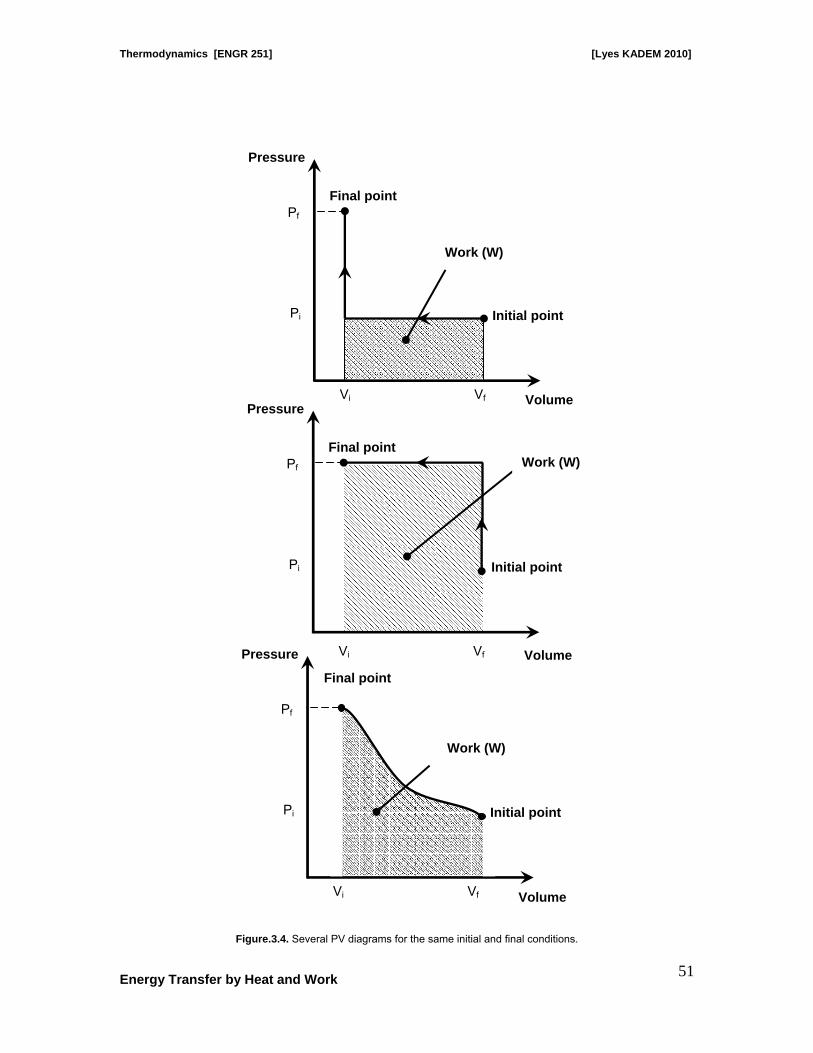
An important thing to realize is that this has significant impact on how much work is done by a particular process between a given (Pi,Vi) and (Pf,Vf). If you look at Fig.3.4, you’ll see just three of many possible PV-processes between (Pi,Vi) and (Pf,Vf), the areas under these curves are different, which means that each has a different W. This is known as a path dependent process. In contrast, a path independent process depends only on the start and end point and not how you get between them – an example is gravitational potential energy it only depends on the change in height, not the path you take in changing that height.
Volume
Pressure
Work = Area = P × (Vf - Vi)
P
Vi Vf Volume
Pressure
Vi Vf
∫= PdVArea
Thermodynamics [ENGR 251] [Lyes KADEM 2010]
Energy Transfer by Heat and Work
51
Figure.3.4. Several PV diagrams for the same initial and final conditions.
Volume
Pressure
Pf
Vi Vf
Pi Initial point
Final point
Volume
Pressure
Pf
Vi Vf
Pi Initial point
Final point
Work (W)
Volume
Pressure
Pf
Vi Vf
Pi
Final point
Initial point
Work (W)
Work (W)

Thermodynamics [ENGR 251] [Lyes KADEM 2010]
Energy Transfer by Heat and Work
52
III.1.1. Some Common works Constant Volume: In a constant volume process dV=0, and so the work W must be 0 also. There is no work in a gas unless it changes its volume. Constant Pressure: Here P is constant, hence:
( )if
V
V
VVPdVPWf
i
−== ∫
Isothermal Expansion: if we use the ideal gas law as P=nRTV, we obtain:
∫=f
i
V
V
dVV
nRTW
Here, R is a constant; n and T (isothermal) are constant, therefore:
( )∫ −==f
i
V
Vif VVnRT
VdVnRTW lnln
III.1.3. Polytropic process
Example A gas in a piston-cylinder assembly undergoes an expansion process for which the relationship between pressure and volume is given by
ctPV n =
The initial pressure is 3 bar, the initial volume is 0.1 m3, and the final volume is 0.2 m3. Determine the work for the process, in kJ if:
a- n = 1.5 b- n = 1.0 c- n = 0

Thermodynamics [ENGR 251] [Lyes KADEM 2010]
Energy Transfer by Heat and Work
53
III.2. Several forms of work III.2.1. Electrical Work If electrons cross the boundaries of the system a work is generated. This work can be computed as:
∫=2
1
dtVIW Where (I) is the current and V is the voltage. III.2.2. Shaft Work In a large majority of engineering devices, the work is transmitted by a rotating shaft. This kind of work can be computed as follow:
TNW &π2= Where, N& is the number of tours per unit of time (tours/min ; tours/second, …) and T is the torque. III.2.3. Spring Work For a linear elastic spring the work can be computed as: ( )2
1222
1 xxkW −= Where; x1 and x2 are the initial and final displacements of the spring, and k is the spring constant.
Example [Schaum’s page 48] The air in a circular cylinder is heated until the spring is compressed 50 mm. Find the work done by the air on the frictionless piston. The spring is initially unstretched.
50 kg
10 cm
K = 2500 N/m

Thermodynamics [ENGR 251] [Lyes KADEM 2010]
Energy Transfer by Heat and Work
54
III.3. Heat Heat can be transmitted through the boundaries of the system only during a non-thermal equilibrium state. Heat is transmitted, therefore, solely due to the temperature difference. The net heat transferred to a system is defined as: ∑ ∑−= outinnet QQQ
Here, Qin and Qout are the magnitudes of the heat transfer values. In most thermodynamic texts, the quantity Q is meant to be the net heat transferred to the system, Qnet. We often think about the heat transfer per unit mass of the system, q.
mQq =
Heat transfer has the units of energy measured in joules (we will use kilojoules, kJ) or the units of energy per unit mass, kJ/kg. Since heat transfer is energy in transition across the system boundary due to a temperature difference, there are three modes of heat transfer at the boundary that depend on the temperature difference between the boundary surface and the surroundings. These are conduction, convection, and radiation. However, when solving problems in thermodynamics involving heat transfer to a system, the heat transfer is usually given or is calculated by applying the first law, or the conservation of energy, to the system. An adiabatic process is one in which the system is perfectly insulated and the heat transfer is zero. III.4. Summary
- Heat is defined as the spontaneous transfer of energy across the boundary of a system due to a temperature difference between the system and its surroundings. There is no external force mediating this process.
- Work is basically defined as any other transfer of energy into or out of the system. The most important form of work in thermodynamics is compressive work, which is due to a change in volume against or due to an external force (or pressure) on a gas.
III.5. The mechanical equivalent of heat (Joule’s experiment) In the 1800s Joule spent a lot of time pondering the quantitative relationship between different forms of energy, looking to see how much is lost in converting from one form to another. As you’ll already know, when friction is present in some mechanical system we always end up losing some of the mechanical energy, and in 1843 Joule did a famous experiment showing that this lost mechanical energy is converted to heat.
As shown in the figure below, Joule’s apparatus consists of water in a thermally insulated vessel. Heavy blocks falling at a constant speed (mechanical energy) are connected to a paddle immersed in the liquid. Some of the mechanical energy is lost to the water as friction between the water and the paddles. This results in an increase in the temperature of the water, as measured by a thermometer immersed in the water. If we ignore the energy lost in the bearings and through the walls, then the loss in gravitational potential energy associated with the blocks equals the work done by the paddles on the water. By varying the conditions of the experiment, he noticed that the loss in mechanical energy 2mgh was proportional to the increase in water temperature ∆T, with a proportionality constant 4.18J/°C. This was one of the key experiments leading up to the discovery of the 1st law

Thermodynamics [ENGR 251] [Lyes KADEM 2010]
Energy Transfer by Heat and Work
55
of thermodynamics.
James Prescott Joule, (December 24, 1818 – October 11, 1889) was an English physicist, born in Sale, near Manchester. Joule studied the nature of heat, and discovered its relationship to mechanical work . This led to the theory of conservation of energy, which led to the development of the first law of thermodynamics. The SI unit of work, the joule, is named after him. He worked with Lord Kelvin to develop the absolute scale of temperature, made observations on magnetostriction, and found the relationship between the flow of current through a resistance and the heat dissipated, now called Joule's law.

CHAPTER IV
First Law of Thermodynamics

Thermodynamics [ENGR 251] [Lyes KADEM 2010]
First Law of Thermodynamics
56
CHAPTER IV
First Law of Thermodynamics
IV.1. First Law of thermodynamics for a closed system
The first law of thermodynamics is usually written as:
WQE −=Δ
The variation in energy = Heat - Work Where Q is heat; W is work and the term E includes numerous types of energy: Internal energy U=U(T,P) It is the form of stored energy which can
be directly influenced by a heat transfer. It is the energy stored microscopically in two forms: as the kinetic energies due to random molecular translations, vibrations and rotations, and as potential energy arising from forces between molecules.
Kinetic energy 2
21 mVKE = Due to the velocity of the system
Potential energy mgzPE = Due to the elevation of the system in a gravitational field.
and:
...+++= PEKEUE You can add other terms (atomic, electromagnetic, chemical, …) to the expression of energy. However, we will usually limit ourselves to the three terms above. It is important to note that this is the most frequent version of the first law of thermodynamics (with minus sign). This is because when people dealt with heat engines, they cared about heat in and work out. You may also find a version with a (+) sign [ΔE=Q+W], this means that the convention of work in and out is not the same. The first law can be also written under the instantaneous time rate form as:
WQdtdE && −=
It is also interesting to note that the first law can not be derived; no algebra can be used to show how it is obtained. This is because it is a blind observation about how the world seems to work.
Note The relative magnitude of the three components of energy (U; KE; PE) is often quite different. The statement of a problem should give a quick clue to which types of terms will predominate. Modest velocities will result in negligible changes in kinetic energy. Similarly, small changes in elevation will result in negligible changes in potential energy.
Thermodynamics [ENGR 251] [Lyes KADEM 2010]
First Law of Thermodynamics
57
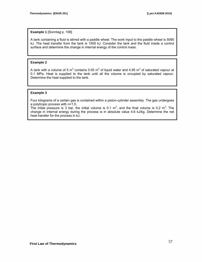
Example 1 [Sonntag p. 108] A tank containing a fluid is stirred with a paddle wheel. The work input to the paddle wheel is 5090 kJ. The heat transfer from the tank is 1500 kJ. Consider the tank and the fluid inside a control surface and determine the change in internal energy of the control mass.
Example 2 A tank with a volume of 5 m3 contains 0.05 m3 of liquid water and 4.95 m3 of saturated vapour at 0.1 MPa. Heat is supplied to the tank until all the volume is occupied by saturated vapour. Determine the heat supplied to the tank.
Example 3 Four kilograms of a certain gas is contained within a piston-cylinder assembly. The gas undergoes a polytropic process with n=1.5. The initial pressure is 3 bar, the initial volume is 0.1 m3, and the final volume is 0.2 m3. The change in internal energy during the process is in absolute value 4.6 kJ/kg. Determine the net heat transfer for the process in kJ.

Thermodynamics [ENGR 251] [Lyes KADEM 2010]
First Law of Thermodynamics
58
IV.2. First Law of thermodynamics for a control volume
IV.2.1. Mass rate balance When analyzing a control volume, the first reflex is to apply the conservation of mass. At each instant the following principle must be valid:
eiCV mm
dtdm
&& −= Where the term on the left side represents the time rate of change of mass contained within the control volume at time (t); and im& is the time rate of flow of mass IN across inlet (i) at time (t); and and em& is the time rate of flow of mass OUT across exit (e) at time (t) (see Figure.4.1).
Figure.4.1. Control volume for a single inlet and a single exit.
The above formulation is valid for one inlet and one outlet. However, in general, there may be several locations on the boundary through which mass enters or exits. In this case, the general form is:
∑∑ −=e
ei
iCV mm
dtdm
&& IV.2.2. Computation of the mass flow rate The mass flow rate can be computed under the following general form:
dAVmd nρ=&
Where ρ is the fluid density; Vn is the normal velocity and dA is surface element. By integration we get:
∫=A
n dAVm ρ&
For the special case of a one-dimensional flow, where the velocity profile is flat and normal to the surface (A) and the surface A does not change with time, we can compute the mass flow rate using the following expression:
υρ AVAVm n
n ==&
IV.2.2.1. Computation of the mass flow rate for a steady flow In the particular case of a steady flow meaning that all properties are unchanging in time, the left term in the general expression of the mass rate balance vanishes. We obtain, therefore, the following expression:
∑∑ −=
ee
ii mm &&0
Exit (e)
Inlet (i)
dtdmCV
im&
em&

Thermodynamics [ENGR 251] [Lyes KADEM 2010]
First Law of Thermodynamics
59
Or
∑∑ =
ee
ii mm &&
IV.2.2.3 First Law of thermodynamics for a control volume
If we consider one inlet and one exit, the energy balance can be written under the following form:
⎟⎟⎠
⎞⎜⎜⎝
⎛++−⎟⎟
⎠
⎞⎜⎜⎝
⎛+++−= e
eeei
iii
CV gzVumgzVumWQdt
dE22
22
&&&&
Now we will try to write this energy balance under an alternative form that is more convenient for our applications. This will be done, first by writing the term W& under another form where we are able to separate the work associated with the fluid pressure as mass is introduced at the inlets and removed at exits from the work due to all other effects (rotating shaft, electrical effects, …). This latest term will be denoted CVW& .
The first term due to pressure can be written under the following form:
( )VPAWPressure =&
Where V is the velocity.
Therefore, the total work can be expressed under the following form:
( ) ( ) iiieeeCV VAPVAPWW −+= &&
Here note that the work at the exit has a positive sign and the work at the inlet has a negative sign.
As we have, for a one-dimensional flow:
υυ
mAVVA
m && =⇔=
Then,
( ) ( )iiieeeCV PmPmWW υυ &&&& −+=
If we replace this expression in the energy balance, we can get:
Example 4 A feedwater heater operating at steady state has two inlets and one exit. At inlet 1, water vapour enters at P1=7 bar, T1=200°C with a mass flow rate of 40 kg/s. At inlet 2, liquid water at P2=7 bar, T2=40°C enters through an area A2=25 cm2. Saturated liquid at 7 bar exits at 3 with a volumetric flow rate of 0.06 m3/s. Determine the mass flow rates at inlet 2 and at the exit, in kg/s, and the velocity at inlet 2, in m/s.

Thermodynamics [ENGR 251] [Lyes KADEM 2010]
First Law of Thermodynamics
60
⎟⎟⎠
⎞⎜⎜⎝
⎛+++−⎟⎟
⎠
⎞⎜⎜⎝
⎛++++−= e
eeeeei
iiiiiCVCV
CV gzVPumgzVPumWQdt
dE22
22
υυ &&&&
It is interesting now to introduce the property: specific enthalpy as,
υPuh +=
We can, therefore, write the energy balance under the form:
⎟⎟⎠
⎞⎜⎜⎝
⎛++−⎟⎟
⎠
⎞⎜⎜⎝
⎛+++−= e
eeei
iiiCVCV
CV gzVhmgzVhmWQdt
dE22
22
&&&&
Note that the introduction of enthalpy was only for convenience.
Now, for several inputs and exists, the general form for the first law of thermodynamics for a control volume is:
∑∑ ⎟⎟⎠
⎞⎜⎜⎝
⎛++−⎟⎟
⎠
⎞⎜⎜⎝
⎛+++−=
ee
eee
ii
iiiCVCV
CV gzVhmgzVhmWQdt
dE22
22
&&&&
For a steady state, we obtain the following form:
44444 344444 21
&&
4444 34444 21
&&
outEnergy
ee
eeeCV
inEnergy
ii
iiiCV gzVhmWgzVhmQ ∑∑ ⎟⎟
⎠
⎞⎜⎜⎝
⎛+++=⎟⎟
⎠
⎞⎜⎜⎝
⎛+++
22
22

Thermodynamics [ENGR 251] [Lyes KADEM 2010]
First Law of Thermodynamics
61
IV.3. Illustrations
IV.3.1. Nozzles and diffusers
A nozzle is a flow passage of varying cross-sectional area in which the velocity of a gas or liquid increases in the direction of flow. A diffuser is the inverse (decrease in velocity).
Figure.4.2. Nozzle and diffuser.
IV.3.1. Turbines
A turbine is a device in which work is developed as a result of a gas or liquid passing through a set of blades attached to a shaft free to rotate.
Example 5 Steam enters a converging-diverging nozzle operating at steady state with P1=40 bar, T1=400°C, and a velocity of 10 m/s. The steam flows through the nozzle with negligible heat transfer and no significant change in potential energy. At the exit, P2=15 bar, and a velocity of 665 m/s. the mass flow rate is 2 kg/s. Determine the exit area of the nozzle, in m2.
Example 6 Steam enters a turbine operating at steady state with a mass flow rate of 4600 kg/h. The turbine loses 63.1 kW of heat to the surroundings. At the inlet, the pressure is 60 bar, the temperature is 400°C, and the velocity is 10 m/s. At the exit, the pressure is 0.1 bar, the quality is 0.9 (90%), and the velocity is 50 m/s. Calculate the power of the turbine in kW.

Thermodynamics [ENGR 251] [Lyes KADEM 2010]
First Law of Thermodynamics
62
Figure.4.3. Steam turbine.
V.3.2. Compressors and pumps Compressors are devices in which work is done to increase the pressure of a GAS. Pumps are devices in which work is done to increase the pressure of a LIQUID. IV.3.3. Heat exchangers Devices that transfer energy between fluids at different temperatures by heat transfer.
Example 7 Air enters a compressor operating at steady state pressure of 1 bar, a temperature of 290 K, and a velocity of 6 m/s through an inlet with an area of 0.1 m2. At the exit, the pressure is 7 bar, the temperature is 450 K, and the velocity is 2 m/s. Heat transfer from the compressor to its surroundings occurs at a rate of 180 kJ/min. Employing the ideal gas model, calculate the power input to the compressor, in kW.
Example 8 Steam enters the condenser of a vapor power plant at 0.1 bar with a quality of 0.95 and condensate exists at 0.1 bar and 45°C. Cooling water enters the condenser in a separate stream as a liquid at 20°C and exists as a liquid at 35°C with no change in pressure. Heat transfer from the outside of the condenser can be ignored. For steady-state operation, determine:
- the ratio of the mass flow rate of the cooling water to the mass flow rate of the condensing stream.

Thermodynamics [ENGR 251] [Lyes KADEM 2010]
First Law of Thermodynamics
63
Figure.4.4. Phase change in a boiler. IV.3.4. Cycles analysis IV.3.4.1. Rankine Cycle Rankine cycle is the ideal cycle for a steam power plant.
Figure.4.5. Rankine cycle.
Example 9 Consider a simple steam power plant with the following data: Location Pressure Temperature or Quality Leaving boiler 2.0 MPa 300°C Entering the turbine 1.9 Mpa 290°C Leaving turbine, entering condenser 15 kPa 90% Leaving condenser, entering pump 14 kPa 45°C Pump work = 4kJ/kg Determine the following quantities per kilogram flowing through the unit: - Heat transfer in line between boiler and turbine. - Turbine work. - Heat transfer in condenser. - Heat transfer in boiler.

Thermodynamics [ENGR 251] [Lyes KADEM 2010]
First Law of Thermodynamics
64
IV.3.4.2. Brayton Cycle Brayton cycle is the ideal cycle for a gas turbine power plant.
Figure.4.6. Brayton cycle.
`
Figure.4.7. Gas turbine. GE H series power 480 MW.
Example 10 In an air-standard Brayton cycle the air enters the compressor at 0.1 Mpa and 15°C. The pressure leaving the compressor is 1.0 Mpa, and the maximum temperature in the cycle is 1100°C. If you consider that the processes through the compressor and the turbine are polytropic (with n=1.4) and the heat transfer processes are isobaric, determine: - The pressure and the temperature at each point in the cycle. - The compressor work, turbine work, and cycle efficiency.

Thermodynamics [ENGR 251] [Lyes KADEM 2010]
First Law of Thermodynamics
65
IV.3.4.2. OTTO Cycle Definitions: BDC: bottom dead center (maximum volume). TDC: top dead center (clearance volume). Bore: diameter of the piston. Stroke: the distance the piston travels in one direction. Mean effective pressure (MEP): the pressure that if acting on the piston during the power stroke, would produce an amount of work equal to that actually done during the entire cycle.
( )TDCBDCcycle VVMEPW −=
( )TDCBDC
cycle
VVW
MEP−
=
Compression ratio (r):
1>=TDCatairthebyoccupiedVolumeBDCatairthebyoccupiedVolumer
Figure.4.8. Otto cycle parameters
TDC
BDC Bore
Stro
ke

Thermodynamics [ENGR 251] [Lyes KADEM 2010]
First Law of Thermodynamics
66
Example 11 The compression ratio (V1/V2) in an air-standard Otto cycle is 10. At the biginning of the compression stroke the pressure is 0.1 MPa and the temperature is 15°C. The heat transfer to the air per cycle is 1800 kJ/kg air. If you consider compression and the expansion as polytropic (with n=1.4) and the heat transfer processes are isochoric, determine: - The pressure and the temperature at each point in the cycle. - The thermal efficiency.
Nikolaus August Otto (June 14, 1832 - January 28, 1891) was the German inventor of the internal-combustion engine, the first engine to burn fuel directly in a piston chamber. Up until his invention, all engines were external-combustion engines and fuel was burned in a separate compartment. Otto's first atmospheric engine was completed in May 1867. Five years later Gottlieb Daimler and Wilhelm Maybach joined his company for a while and together they produced the idea of the four-stroke cycle or, Otto cycle engine, which was first described in 1876. The Otto Cycle engine patent was invalidated in 1886 when it was discovered that another inventor, Alphonse Beau de Rochas, had already described the four-stroke cycle principle in a privately published pamphlet. (ref. Wikipedia)

Thermodynamics [ENGR 251] [Lyes KADEM 2010]
67
First Law of Thermodynamics: Unsteady formulation I. Energy balance for unsteady-flow processes In this case, the amount of mass and energy within the control volume do change with time. So,
NEVER write 0=dtdm
or 0=dtdE
, hence:
For an unsteady-flow process: 0≠dtdm
and 0≠dtdE
Under this hypothesis, and if we consider that variations in kinetic and potential energies can be neglected, the first law can be written under the following form:
( ) ( ) ( )systemoutoutoutoutiiinin umumhmWQhmWQ 1122 −=++−++ ∑∑
PROBLEM I A pressure cooker is initially half-filled with liquid water. If the pressure cooker is not to run out of liquid water for 1 h, the highest rate of heat transfer allowed is to be determined.
PROBLEM II A tank of 2 m3 volume contains saturated ammonia at a temperature of 40°C. Initially the tank contains 50% liquid and 50% vapor by volume. Vapor is withdrawn from the top of the tank until the temperature is 10°C. Assuming that only vapor leaves and that the process is adiabatic, calculate the mass of ammonia that is withdrawn.

CHAPTER V
Second Law of Thermodynamics

Thermodynamics [ENGR 251] [Lyes KADEM 2010]
Second Law of Thermodynamics
68
CHAPTER V
Second Law of Thermodynamics
The first law of thermodynamics is a representation of the conservation of energy. It is a necessary, but not a sufficient, condition for a process to occur. Indeed, no restriction is imposed by the first law on the direction of the process: this is the role of the second law.
To illustrate this, let us assume the processes below, in your opinion, without any intervention from you, what is the most probable process (from left to right or the inverse):
g ?
?
HOT
COLD
?

Thermodynamics [ENGR 251] [Lyes KADEM 2010]
Second Law of Thermodynamics
69
Consider now the following arrangement:
Allowing the weight to fall will turn the paddlewheel which will do work on the fluid system. Initially this may increase the kinetic energy of the fluid as it churns, but in time the circulation will stop. When this happens the temperature of the fluid will rise and the heat will be transferred to the surroundings. From a 1st Law perspective there is no reason why one could not simply supply this same amount of heat to the fluid so that the paddlewheel would turn and the weight would be raised. However, no one has ever built a successful engine based on this principle. It simply wouldn’t work. The 2nd Law provides us with a basis to determine why such a process isn’t feasible.
I. Heat Engines
While the 2nd Law of Thermodynamics is applicable to a wide range to topics, much of our understanding of the principle comes from the study of heat engines. We will therefore use engines as a basis for much of our study.
Liquid
Paddlewheel
Cooler
Compressor
Combustor
Turbine WC WT
1
2 3
4
Q23=Qin
Q14=Qout
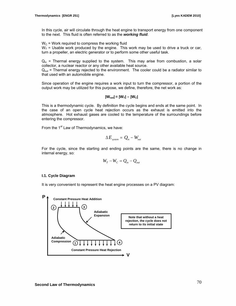
Thermodynamics [ENGR 251] [Lyes KADEM 2010]
Second Law of Thermodynamics
70
In this cycle, air will circulate through the heat engine to transport energy from one component to the next. This fluid is often referred to as the working fluid. WC = Work required to compress the working fluid WT = Usable work produced by the engine. This work may be used to drive a truck or car, turn a propeller, an electric generator or to perform some other useful task. Qin = Thermal energy supplied to the system. This may arise from combustion, a solar collector, a nuclear reactor or any other available heat source. Qout = Thermal energy rejected to the environment. The cooler could be a radiator similar to that used with an automobile engine. Since operation of the engine requires a work input to turn the compressor, a portion of the output work may be utilized for this purpose, we define, therefore, the net work as:
|Wnet| = |WT| – |WC| This is a thermodynamic cycle. By definition the cycle begins and ends at the same point. In the case of an open cycle heat rejection occurs as the exhaust is emitted into the atmosphere. Hot exhaust gases are cooled to the temperature of the surroundings before entering the compressor. From the 1st Law of Thermodynamics, we have:
ΔE Q Wsystem in out= − For the cycle, since the starting and ending points are the same, there is no change in internal energy, so:
outinCT QQWW −=−
I.1. Cycle Diagram It is very convenient to represent the heat engine processes on a PV diagram:
Note that without a heat rejection, the cycle does not
return to its initial state
Constant Pressure Heat Addition
Constant Pressure Heat Rejection
Adiabatic Compression
Adiabatic Expansion
P
V
1 4
3 2

Thermodynamics [ENGR 251] [Lyes KADEM 2010]
Second Law of Thermodynamics
71
I.2. Thermal Efficiency of a heat engine The efficiency of a heat engine can be defined as the ratio of the useful work out (the net work) to the energy that must be input in (the energy that we pay for).
in
net
QW
=η
Since we have that Wnet = Qin – Qout, we may substitute into the above equation and find:
( )in
out
in
outin
QQQ
−=−
= 1η
It is probably not too surprising that we want to minimize the fraction of rejected heat in the last part of the equation in order to attain the maximum efficiency.
I.3. Second law of Thermodynamics: Kelvin-Planck statement
In the drawing above, a piston-cylinder contains a gas at 30oC. A weight is placed on the piston. Heat is then added to the gas from a reservoir at 100oC so that the gas expands. As the gas expands it does work to raise the weight and piston. The weight now is at a higher potential energy than at state one. We slide the weight off of the piston at the higher elevation. Assume that the frictional forces in sliding the weight are negligible. Now, we wish to raise a second weight. That is, we wish the heat engine to continue to do work. The gas inside the cylinder is still heated and will not return to its initial position unless the gas is cooled. If you consider the gas turbine cycle and the piston-cylinder arrangement, in both cases we have seen that it is necessary to reject heat at the end of the work process in order to bring the cycle to its initial state and repeat the process. We generalize this observation as the 2nd Law of Thermodynamics:
Reservoir at 100oC
GAS 90oC GAS
30oCGAS 30oC
Reservoir at 20oC
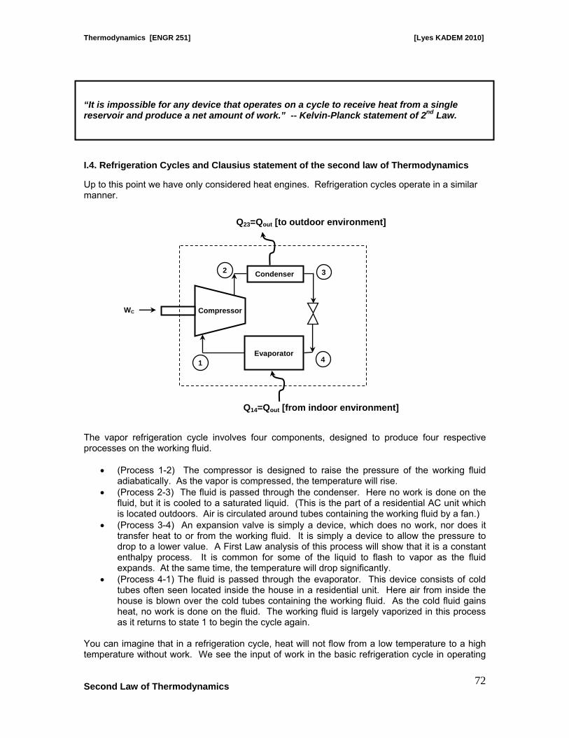
Thermodynamics [ENGR 251] [Lyes KADEM 2010]
Second Law of Thermodynamics
72
“It is impossible for any device that operates on a cycle to receive heat from a single reservoir and produce a net amount of work.” -- Kelvin-Planck statement of 2nd Law.
I.4. Refrigeration Cycles and Clausius statement of the second law of Thermodynamics Up to this point we have only considered heat engines. Refrigeration cycles operate in a similar manner. The vapor refrigeration cycle involves four components, designed to produce four respective processes on the working fluid.
• (Process 1-2) The compressor is designed to raise the pressure of the working fluid adiabatically. As the vapor is compressed, the temperature will rise.
• (Process 2-3) The fluid is passed through the condenser. Here no work is done on the fluid, but it is cooled to a saturated liquid. (This is the part of a residential AC unit which is located outdoors. Air is circulated around tubes containing the working fluid by a fan.)
• (Process 3-4) An expansion valve is simply a device, which does no work, nor does it transfer heat to or from the working fluid. It is simply a device to allow the pressure to drop to a lower value. A First Law analysis of this process will show that it is a constant enthalpy process. It is common for some of the liquid to flash to vapor as the fluid expands. At the same time, the temperature will drop significantly.
• (Process 4-1) The fluid is passed through the evaporator. This device consists of cold tubes often seen located inside the house in a residential unit. Here air from inside the house is blown over the cold tubes containing the working fluid. As the cold fluid gains heat, no work is done on the fluid. The working fluid is largely vaporized in this process as it returns to state 1 to begin the cycle again.
You can imagine that in a refrigeration cycle, heat will not flow from a low temperature to a high temperature without work. We see the input of work in the basic refrigeration cycle in operating
Evaporator
Compressor
Condenser
WC
1
2 3
4
Q23=Qout [to outdoor environment]
Q14=Qout [from indoor environment]

Thermodynamics [ENGR 251] [Lyes KADEM 2010]
Second Law of Thermodynamics
73
the compressor. This principle is accepted as an alternate statement of the Second Law of Thermodynamics. “It is impossible to construct a device that operates in a cycle and produces no effect other than the transfer of heat from a lower-temperature body to a higher-temperature body.” -- Clausius statement of 2nd Law. The two statements of the 2nd Law can be shown to be equivalent.
I.4.1. Coefficient of performance When describing heat engines, we introduced the concept of engine efficiency as the desired output divided by the energy input. Similarly, we define the coefficient of performance (COP) of a refrigerator:
1423
1414
QQQ
WQ
InputRequiredOuputDesiredCOP
net −===
The definition is basically the same as that of thermal efficiency. The primary reason for the change in terminology is that a COP: is often greater than 1. The term is used to avoid speaking of any efficiency greater than 100%. I.5. Reversibility Consider a system of pulleys and weights as shown:
Practical statement of the second law of Thermodynamics In the normal course of events, when things are not actively maintained, they deteriorate. Suns burn out, mountains crumble, cars rust, houses fall down, etc. The reverse process does not happen without intervention. You might buy an old, rusty car and restore it, but it will take work. In a like fashion, process involving an energy transfer will only occur in such a way so as to decrease the quality of energy. We can, within a finite control volume, transfer energy to the system so as to increase the quality of energy within that system. However, the work that we input required that we decrease the quality of energy from an area outside the system. When we consider the universe as a whole, the quality of energy in the universe has still deteriorated.
W + δW W

Thermodynamics [ENGR 251] [Lyes KADEM 2010]
Second Law of Thermodynamics
74
In order for the weight on the right to raise the weight on the left, it is essential that W+ δW > W. How large must δW be? Well, it must be large enough that it compensates for the effects of friction in the pulley, the friction associated with the flexing of the cable, etc. If we use very good bearings, then the required extra weight on the right may approach zero. Can it reach zero? No, this would result in static equilibrium and the weights will no move. It is essential that δW be greater than zero; it may approach, but never reach zero, even with perfect bearings. We see that, in order for the process of raising the left weight to occur, the loss in potential energy on the right must be greater than the gain in potential energy on the left. As an idealization only, we may assume that the weight δW may be so small that it can be treated as zero. In such a case, the weight on the right and left are equal and the direction that the pulley moves would be completely reversible. Such processes never occur in nature, but may be approached in the limit.

Thermodynamics [ENGR 251] [Lyes KADEM 2010]
Second Law of Thermodynamics
75
II. Carnot Cycle The Carnot cycle was first proposed in 1824, by Sadi Carnot. The interest in the cycle is largely theoretical, as no practical Carnot cycle engine has yet been built. Nevertheless, it can be shown to be the most efficient cycle possible, so that considerable attention has been given at discovering ways of making the more practical cycles look, as much as possible, like the Carnot.
Process 1-2 Process 2-3 Process 3-4 Process 4-1 (Process 1-2) A constant temperature heat addition. (Process 2-3) An adiabatic expansion (Process 3-4) A constant temperature heat rejection. (Process 4-1) An adiabatic compression
Energy Source @
TH
TH = Const
TH
TL
TL = Const
Insulation
Energy Sink @ TL
TH
TL
Insulation
P
v
TH
TL
4
1
2
3

Thermodynamics [ENGR 251] [Lyes KADEM 2010]
Second Law of Thermodynamics
76
II.1. Carnot Cycle Efficiency Like other heat engines, the Carnot cycle efficiency can be attained from the relationship:
in
out
in
outin
in
inout
in
net
QQQ
QWW
QW
−=−
=−
== 1η
II.1.1. Carnot cycle principles 1. The efficiency of an irreversible heat engine is always less than the efficiency of a reversible one operating between the same two reservoirs. 2. The efficiencies of all reversible heat engines operating between the same two reservoirs are the same.
Reversible Heat Engine
C
High Temperature Energy Reservoir, TH
Low Temperature Energy Reservoir, TC
WC
Reversible Heat Engine
A
Reversible Heat Engine
B
WC
WA
WB
TB
QA
QC
QA
QB
QC

Thermodynamics [ENGR 251] [Lyes KADEM 2010]
Second Law of Thermodynamics
77
If we consider the Carnot cycle above, since a control volume could be drawn about engines A & B together, they may be considered as a single reversible engine. The efficiency of Engine A&B must be the same as that of Engine C since both are reversible. Also
WA + WB = WC Since energy reservoirs are characterized by their temperatures, the thermal efficiency of reversible heat engines is a function of the reservoir temperatures only. That is,
),( LHH
L TTfQQ
=
Applying this idea to the three engines separately, QA/QC = f(TA, TC), QA/QB = f(TA, TB), QB/QC = f(TB, TC) For the efficiency of A&B to be equal to that of C f(TA, TC) = f(TA, TB)⋅ f(TB, TC) A careful examination of this equation reveals that the left hand side is a function of TA and TC, and therefore the right hand side must also be a function of TA and TC only and not, TB. This condition will be satisfied only if the function has the following form: Φ(TA)/ Φ(TC) = [Φ(TA)/ Φ(TB)]⋅[Φ(TB)/ Φ(TC)] From this relationship Kelvin proposed a temperature scale in which Φ(T) = T, such that:
H
L
TT
−= 1η
II.1.2. Applications of the Carnot Cycle a. Carnot Cycle Engine
From the first law of thermodynamics:
WQQ LH&&& +=
High Temperature region
Low Temperature region
Carnot Cycle
HQ&
LQ&
W&

Thermodynamics [ENGR 251] [Lyes KADEM 2010]
Second Law of Thermodynamics
78
From the definition of efficiency, we find for the Carnot engine:
H
L
QQ&
&−=1η
Using the thermodynamic temperature scale:
H
L
TT
−=1η
b. Carnot Cycle Refrigerator From the definition of Coefficient of Performance (COP), we find for the Carnot refrigeration cycle:
1
1
−=
−==
L
HLH
LL
QQQQ
QWQCOP
&
&&&
&
&
&
Using the thermodynamic temperature scale:
1
1
−=
L
H
TT
COP
From the first law of thermodynamics:
WQQ LH&&& +=
High Temperature region
Low Temperature region
Carnot Cycle
HQ&
LQ&
W&

Thermodynamics [ENGR 251] [Lyes KADEM 2010]
Second Law of Thermodynamics
79
C. Carnot Cycle Heat Pump From the definition of Coefficient of Performance (COP), we find for the Carnot refrigeration cycle:
H
LLH
HH
QQQQ
QWQCOP
&
&&&
&
&
&
−=
−==
1
1
Using the thermodynamic temperature scale:
H
L
TT
COP−
=1
1
II.2. Applications Example 1 An inventor claims to have developed a power cycle capable of delivering a net work output of 410 kJ for an energy input by heat transfer of 1000 kJ. The system undergoing the cycle receives the heat transfer from hot gases at a temperature of 500 K and discharges energy by heat transfer to the atmosphere at 300 K. Evaluate this claim. Example 2 When a fridge stands, in a room at 20°C, the motor has to extract 500 W of heat from the cabinet at 4°C to compensate for less than perfect insulation. How much power must be supplied to the motor if its efficiency is 80% of the maximum efficiency?
From the first law of thermodynamics:
WQQ LH&&& +=
High Temperature region
Low Temperature region
Carnot Cycle
HQ&
LQ&
W&

Thermodynamics [ENGR 251] [Lyes KADEM 2010]
Second Law of Thermodynamics
80
Example 3 An ideal or Carnot heat pump is used to heat a house to TH=294 K, how much work must be done by the pump to deliver QH=3350 J of heat into the house when the outdoor temperature is 273 K and 252 K. Example 4 A Carnot power cycle using air as a working fluid has a thermal efficiency of 40%. At the beginning of isothermal expansion, the pressure is 620 kPa, and the specific volume is 0.1 m3/kg. If the heat input for the cycle is 50 kJ/kg, determine:
- The highest and the lowest temperature for the cycle. - The work and heat for each process of the cycle.
Assume air to be an ideal gas with constant specific heats.

CHAPTER VI
Entropy

Thermodynamics [ENGR 251] [Lyes KADEM 2010]
Entropy
81
CHAPTER VI
ENTROPY In the previous chapter, we tried to understand the 2nd law of thermodynamics from a conceptual perspective. In this chapter, we begin to consider these concepts in a more analytical manner. In the process, we will introduce a new property, ENTROPY, which is defined as follows:
dSQT rev
=δ
That is, a differential change in entropy corresponds to a differential quantity of heat being transferred divided by the temperature at which is it transferred in a reversible process. I. Clausius Inequality: Recall the Kelvin-Plank statement of the 2nd Law. “It is impossible for any device that operates on a cycle to receive heat from a single reservoir and produce a net amount of work.” Clausius proceeded to consider a device, shown below, which violates the 2nd Law. Work is produced, but the device receives heat from a single reservoir Let us apply the 1st Law for the control volume:
ΔE Q Wsystem in out= − The total work output is the sum of that for the system and the heat engine:
δWT = (δWrev + δWsys)
Thermal reservoir @ TR
Reversible Heat
Engine
RQδ
Qδ
revW&δ
sysW&δ System

Thermodynamics [ENGR 251] [Lyes KADEM 2010]
Entropy
82
For an infinitesimal part of the engine cycle we write:
TRsystem WQdE δδ −= Since the cyclic device is a reversible heat engine, it follows from the definition of the thermodynamical temperature scale that:
δQR/δQ = TR/T Then, we can obtain:
TR
system WTTQdE δδ −=
Consider the operation of the device through a complete engine cycle. For a cycle the energy of the control volume must return to its initial value so that the energy term drops out.
0 = −∫TQT
WR T
δ
Or
W TQTT R= ∫δ
As noted previously, if the total work is positive then this device would violate the Kelvin-Plank statement of the 2nd Law. It follows that the total work must be zero or negative.
δQT∫ ≤ 0
Now let us run the engine in reverse. If the path for the cycle is reversed, then the sign of the integral is reversed and the integral will become greater than or equal to zero. This would likewise result in a violation of the 2nd Law. The only way that the process can be reversed is if the integral gives a value of zero. In the special case that the cyclic integral is zero, then the quantity under the integral, δQ/T, returns to its initial value during the cycle. It behaves like a thermodynamic property. Then, the entropy (S):
dSQT rev
=δ
If the integral of δQ/T about a cycle is equal to zero, then the process is said to be reversible

Thermodynamics [ENGR 251] [Lyes KADEM 2010]
Entropy
83
II. Increase in Entropy Principle
Since δQ/T is zero for a reversible process and less than zero for an irreversible process, then
δ δQT
QT rev
∫ ≤ ∫
and
δQT
dS∫ ≤
Finally, for any process between two states:
dSQT
≥δ
or
S SQT2 1
1
2
− ≥ ∫δ
or
S SQT
Sgenerated2 11
2
− = +∫δ
And this can be considered as a quantative statement of the second law.
III. Gibbs equations or Tds Relationships From the 1st Law for a closed system:
dE Q Wsystem in out= −δ δ
Neglecting kinetic and potential energy, this reduces to:
dU Q Wsystem in out= −δ δ
From the definition of entropy, S, we have:
δQ T dSrev = ⋅
Example Air is compressed by a 8 kW compressor from P1 to P2. The air temperature is maintained constant at 25oC during this process as a result of heat transfer to the surrounding medium at 10oC. Determine the rate of entropy change of the air. State the assumptions made in solving this problem.
A process can only occur if the entropy generated is greater than or equal to zero

Thermodynamics [ENGR 251] [Lyes KADEM 2010]
Entropy
84
For a simple compressible substance, we can write a reversible work term as:
δW = P dV After substitution and rearranging T dS = dU + P dV The alternate form of this relationship is obtained using enthalpy:
H = U + P V So that after differentiation,
dH = dU +P dV + V dP Replacing the last two terms in the above T-dS relationship: T dS = dH – V dP These T-dS relationships form the basis for evaluation of entropy as a thermodynamic property.
IV- Entropy for Liquids & Solids & ideal gases IV.1. Entropy for liquids and solids
Normally we expect volume changes to be small as liquids or solids undergo a change in thermodynamic state. Furthermore, Cp ≈ Cv ≈ C so that:
T ds = du + P dv ≈ C dT
Then, ds = C dT/T
or,
IV.2. Entropy for ideal gases
Using the T-ds relationships, we substitute the ideal gas law for the last terms: T ds = du + P dv = Cv dT + R T dv/v and T ds = dh – v dP = Cp dT – R T dP/P
Divide by T and integrate:
s2 – s1 = Cavg ln(T2/T1)

Thermodynamics [ENGR 251] [Lyes KADEM 2010]
Entropy
85
s2 – s1 = Cv,avg ln(T2/T1) + R ln(v2/v1) 1st T-ds relationship and
s2 – s1 = Cp,avg ln(T2/T1) – R ln(P2/P1) 2nd T-ds relationship Note that the above expressions may be placed on a molar basis by dividing by the molecular weight of the particular gas:
ŝ2 – ŝ 1 = Ĉv,avg ln(T2/T1) + (R/M) ln(v2/v1) and
ŝ2 – ŝ 1 = Ĉp,avg ln(T2/T1) – (R/M) ln(P2/P1)
IV.2.1. Isentropic Processes (ΔS = 0) of Ideal Gases Isentropic refers to a process which occurs at constant entropy, s. From the definition of entropy, dS = ∫δQ/T│rev we see that for a reversible, adiabatic process ΔS = 0. Let us take a look at the specific heats relationships:
Cp = Cv + R k = Cp/Cv
From the 1st T⋅dS relationship we developed the following relationship for an ideal gas:
s2 – s1 = Cv,avg ln(T2/T1) + R ln(v2/v1)
For an isentropic process Δs = 0 so that after simplifying and rearranging.
ln(T2/T1) = (R/ Cv,avg)·ln(v1/v2)
then, we have: Cp/Cv = 1 + R/Cv
and k - 1 = R/Cv
Substitute this result into our simplified T-dS relationship:
ln(T2/T1) = (k-1) ln(v1/v2)
Raise both sides to the e power:
1
2
1
1
2
−
⎟⎟⎠
⎞⎜⎜⎝
⎛=
k
vv
TT
1st Isentropic relationship for an ideal gas

Thermodynamics [ENGR 251] [Lyes KADEM 2010]
Entropy
86
For a particular ideal gas P1v1/T1 = R = P2v2/T2
so that v2/v1 = P2T1/ P1T2
Substitute into 1st isentropic relationship
k
k
PP
TT
1
1
2
1
2
−
⎟⎟⎠
⎞⎜⎜⎝
⎛= 2nd Isentropic relationship for an ideal gas
And, P2v2/ P1v1 = (v1/v2) k-1 So that
k
vv
PP
⎟⎟⎠
⎞⎜⎜⎝
⎛=
2
1
1
2 3rd Isentropic relationship for an ideal gas
Example
A 0.5 m3 insulated rigid tank contains 0.9 kg of carbon dioxide at 100 kPa. Now paddle wheel work is done on the system until the pressure in the tank rises to 120 kPa. Determine the entropy change of carbon dioxide during this process in kJ/K. Assume constant specific heats.

Thermodynamics [ENGR 251] [Lyes KADEM 2010]
Entropy
87
V. Steady Flow Work We have previously discussed work from piston-cylinder devices. In this closed system, the work obtained from the fluid can be evaluated as:
W P dV= ⋅∫ However, other devices do create work without lending themselves to this type of piston-cylinder devices (example: turbine). Consider a typical open system as represented by a turbine or a compressor. In these cases there are no moving of the control surfaces.
Let us analyze this sytem: We consider a control volume including the turbine or the compressor.
Conservation of Mass
mmmmmdtdm
outinoutinCV
&&&&& ==⇒−=
Conservation of Energy We will assume steady state (no energy storage inside control volume) and neglect any heat transfer. We will also neglect variations in kinetic and potential energies.
shaftinoutoutinin WQhmhm &&&& −+−=0 Then:
( )outinshaft hhmW −= &&
Motor or
Generator
min mout
Turbine or
Compressor

Thermodynamics [ENGR 251] [Lyes KADEM 2010]
Entropy
88
Second Law Analysis If we do not know how much irreversibility is introduced in the system, we may be interested in finding the maximum possible work.
S SQT
Sgenerated2 11
2
− = +∫δ
Since we assume an adiabatic process then δQ = 0. Further, if we assume that the process is reversible then Sgen = 0, so that
S2 – S1 = 0
If we then recall the 2nd T⋅dS relationship
T dS = dh – v dP
So that, dh = v dP
Substitute this result back into the 1st Law result:
( )( )outinshaft PPvmW −= &&
( )inoutshaft PPVW −−=&
PVWshaft Δ−=&
Please note, this is not the same as VPWshaft Δ=& which we obtained for the closed system. VI. Isentropic Efficiencies of Steady Flow Devices We have been considering the performance of an ideal compressor or ideal turbine, i.e. one which operates both adiabatically and reversibly. However, no real equipment can operate quite so efficiently. We define the efficiency of an adiabatic compressor as:
real
adiabaticreversible
real
adiabaticreversiblecompressor h
hW
WΔ
Δ== ++η
Note: remember that reversible + adiabatic = isentropic (ds = s2-s1=0)
Example Liquid water enters a 10 kW pump at 100 kPa pressure at a rate of 5 kg/s. Determine the highest pressure the liquid water can have at the exit of the pump. Neglect the kinetic and potential energy changes of water and take the specific volume of water to be 0.001m3/kg.

Thermodynamics [ENGR 251] [Lyes KADEM 2010]
Entropy
89
Consider a typical compression process as shown on an h-s (enthalpy - entropy) diagram:
Then 12
12
hhhh s
compressor −−
=η
Now, for a turbine, the definition of efficiency is a little different than for compressors in that the actual work out of a turbine is less than the reversible adiabatic work. In order to ensure that efficiencies are less than 100%, we write:
adiabaticreversible
real
adiabaticreversible
realTurbine h
hW
W++ Δ
Δ==η
Consider a typical process through a turbine as shown on an h-s diagram:
Then 12
12
hhhh
sTurbine −
−=η
s
PH PL
h2 h2s h1 s1 s2s s2
h
h s
PH PL
h1 h2 h2s s1 s2s s2
1
2s 2
1
2
2s
Example Steam enters an adiabatic turbine at 8 MPa and 500oC with a mass flow rate of 3 kg/s and leaves at 30 kPa. The isentropic efficiency of the turbine is 0.90. Neglecting the kinetic energy change of the steam, determine (a) the temperature at the turbine exit and (b) the power output of the turbine.