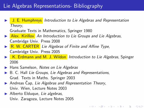
Lie Algebras Representations- Bibliography

I J. E. Humphreys Introduction to Lie Algebras and RepresentationTheory,Graduate Texts in Mathematics, Springer 1980

I Alex. Kirillov An Introduction to Lie Groups and Lie Algebras,Cambridge Univ. Press 2008

I R. W. CARTER Lie Algebras of Finite and Affine Type,Cambridge Univ. Press 2005

I K. Erdmann and M. J. Wildon Introduction to Lie Algebras, Spinger2006

I Hans Samelson, Notes on Lie AlgebrasI B. C. Hall Lie Groups, Lie Algebras and Representations,

Grad. Texts in Maths. Springer 2003I Andreas Cap, Lie Algebras and Representation Theory,

Univ. Wien, Lecture Notes 2003I Alberto Elduque, Lie algebras,

Univ. Zaragoza, Lecture Notes 2005

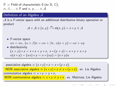
F = Field of characteristic 0 (ex R, C),α, β, . . . ∈ F and x , y , . . . ∈ A

Definition of an Algebra AA is a F-vector space with an additional distributive binary operation orproduct

A×A 3 (x , y)m−→m(x , y) = x ∗ y ∈ A

F-vector spaceαx = xα, (α + β)x = αx + βx , α(x + y) = αx + αydistributivity(x + y) ∗ z = x ∗ z + y ∗ z , x ∗ (y + z) = x ∗ y + x ∗ zα(x ∗ y) = (αx) ∗ y = x ∗ (αy) = (x ∗ y)α

associative algebra ≡ (x ∗ y) ∗ z = x ∗ (y ∗ z),

NON associative algebra ≡ (x ∗ y) ∗ z 6= x ∗ (y ∗ z) , ex. Lie Algebracommutative algebra ≡ x ∗ y = y ∗ x ,NON commutative algebra ≡ x ∗ y 6= y ∗ x , ex. Matrices, Lie Algebra

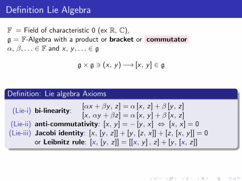
Definition Lie Algebra

F = Field of characteristic 0 (ex R, C),g = F-Algebra with a product or bracket or commutatorα, β, . . . ∈ F and x , y , . . . ∈ g

g× g 3 (x , y)−→ [x , y ] ∈ g

Definition: Lie algebra Axioms

(Lie-i) bi-linearity:[αx + βy , z ] = α [x , z ] + β [y , z ][x , αy + βz ] = α [x , y ] + β [x , z ]

(Lie-ii) anti-commutativity: [x , y ] = − [y , x ] ⇔ [x , x ] = 0(Lie-iii) Jacobi identity: [x , [y , z ]] + [y , [z , x ]] + [z , [x , y ]] = 0

or Leibnitz rule: [x , [y , z ]] = [[x , y ] , z ] + [y , [x , z ]]

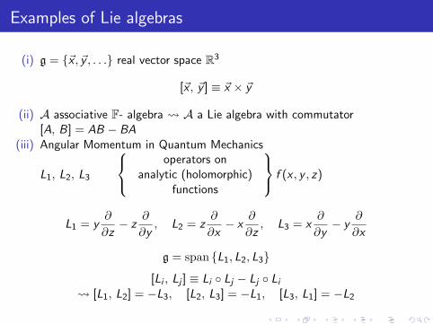
Examples of Lie algebras

(i) g = {~x , ~y , . . .} real vector space R3

[~x , ~y ] ≡ ~x × ~y

(ii) A associative F- algebra A a Lie algebra with commutator[A, B] = AB − BA

(iii) Angular Momentum in Quantum Mechanics

L1, L2, L3

operators on

analytic (holomorphic)functions

f (x , y , z)

L1 = y∂

∂z− z

∂

∂y, L2 = z

∂

∂x− x

∂

∂z, L3 = x

∂

∂y− y

∂

∂x

g = span {L1, L2, L3}

[Li , Lj ] ≡ Li ◦ Lj − Lj ◦ Li [L1, L2] = −L3, [L2, L3] = −L1, [L3, L1] = −L2

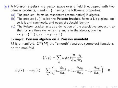
(iv) A Poisson algebra is a vector space over a field F equipped with twobilinear products, · and { , }, having the following properties:

(a) The product · forms an associative (commutative) F-algebra.(b) The product { , }, called the Poisson bracket, forms a Lie algebra, and

so it is anti-symmetric, and obeys the Jacobi identity.(c) The Poisson bracket acts as a derivation of the associative product ·, so

that for any three elements x , y and z in the algebra, one has{x , y · z} = {x , y} · z + y · {x , z}

Example: Poisson algebra on a Poisson manifoldM is a manifold, C∞(M) the ”smooth”/analytic (complex) functionson the manifold.

{f , g} =∑ij

ωij(x)∂f

∂xi

∂j

∂xg

ωij(x) = −ωji (x),∑m

(ωkm

∂ωij

∂xm+ ωim

∂ωjk

∂xm+ ωjm

∂ωki

∂xm

)= 0

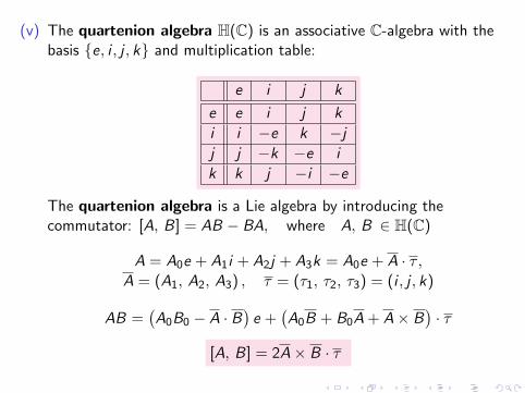
(v) The quartenion algebra H(C) is an associative C-algebra with thebasis {e, i , j , k} and multiplication table:

e i j k

e e i j k

i i −e k −jj j −k −e i

k k j −i −e

The quartenion algebra is a Lie algebra by introducing thecommutator: [A, B] = AB − BA, where A, B ∈ H(C)

A = A0e + A1i + A2j + A3k = A0e + A · τ ,A = (A1, A2, A3) , τ = (τ1, τ2, τ3) = (i , j , k)

AB =(A0B0 − A · B

)e +

(A0B + B0A + A× B

)· τ

[A, B] = 2A× B · τ

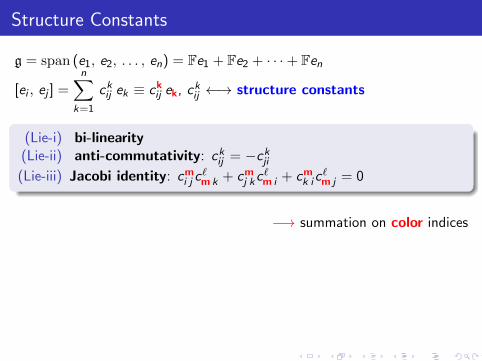
Structure Constants

g = span (e1, e2, . . . , en) = Fe1 + Fe2 + · · ·+ Fen

[ei , ej ] =n∑

k=1

ckij ek ≡ ckij ek, ckij ←→ structure constants

(Lie-i) bi-linearity(Lie-ii) anti-commutativity: ckij = −ckji(Lie-iii) Jacobi identity: cmi j c

`m k + cmj kc

`m i + cmk ic

`m j = 0

−→ summation on color indices

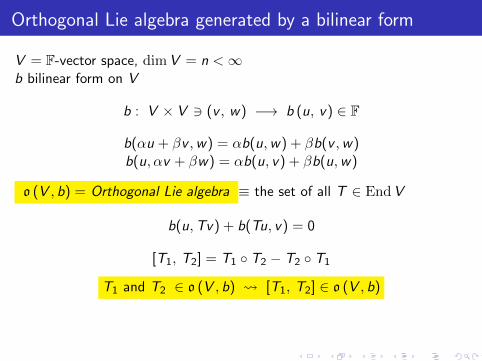
Orthogonal Lie algebra generated by a bilinear form

V = F-vector space, dimV = n <∞b bilinear form on V

b : V × V 3 (v , w) −→ b (u, v) ∈ F

b(αu + βv ,w) = αb(u,w) + βb(v ,w)b(u, αv + βw) = αb(u, v) + βb(u,w)

o (V , b) = Orthogonal Lie algebra ≡ the set of all T ∈ EndV

b(u,Tv) + b(Tu, v) = 0

[T1, T2] = T1 ◦ T2 − T2 ◦ T1

T1 and T2 ∈ o (V , b) [T1, T2] ∈ o (V , b)

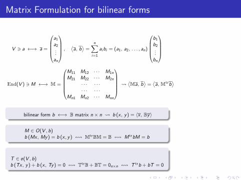
Matrix Formulation for bilinear forms

V 3 a ←→ a =

a1

a2...an

,⟨a, b

⟩=

n∑i=1

aibi = (a1, a2, . . . , an)

b1

b2...bn

End(V ) 3 M ←→ M =

M11 M12 · · · M1n

M21 M22 · · · M2n

· · · · · ·· · · · · ·

Mn1 Mn2 · · · Mnn

⟨Ma, b

⟩=⟨a, Mtrb

⟩

bilinear form b ←→ B matrix n × n b (x , y) = 〈x , By〉

M ∈ O(V , b)b (Mx , My) = b (x , y) ! MtrBM = B ! MtrbM = b

T ∈ o(V , b)b (Tx , y) + b (x , Ty) = 0 ! TtrB + BT = 0n×n ! T trb + bT = 0

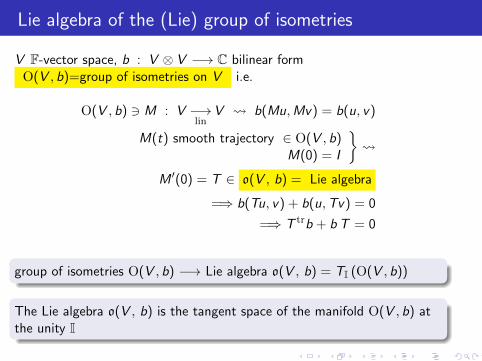
Lie algebra of the (Lie) group of isometries

V F-vector space, b : V ⊗ V −→ C bilinear formO(V , b)=group of isometries on V i.e.

O(V , b) 3 M : V −→lin

V b(Mu,Mv) = b(u, v)

M(t) smooth trajectory ∈ O(V , b)M(0) = I

}

M ′(0) = T ∈ o(V , b) = Lie algebra

=⇒ b(Tu, v) + b(u,Tv) = 0

=⇒ T trb + b T = 0

group of isometries O(V , b) −→ Lie algebra o(V , b) = TI (O(V , b))

The Lie algebra o(V , b) is the tangent space of the manifold O(V , b) atthe unity I

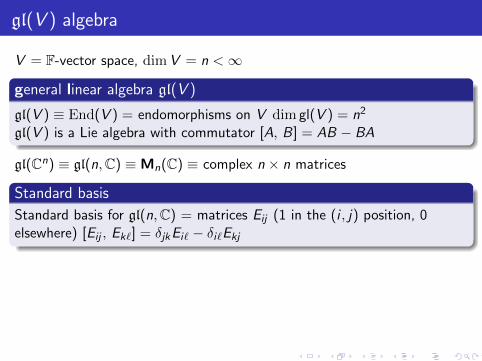
gl(V ) algebra

V = F-vector space, dimV = n <∞

general linear algebra gl(V )

gl(V ) ≡ End(V ) = endomorphisms on V dim gl(V ) = n2

gl(V ) is a Lie algebra with commutator [A, B] = AB − BA

gl(Cn) ≡ gl(n,C) ≡Mn(C) ≡ complex n × n matrices

Standard basis

Standard basis for gl(n,C) = matrices Eij (1 in the (i , j) position, 0elsewhere) [Eij , Ek`] = δjkEi` − δi`Ekj

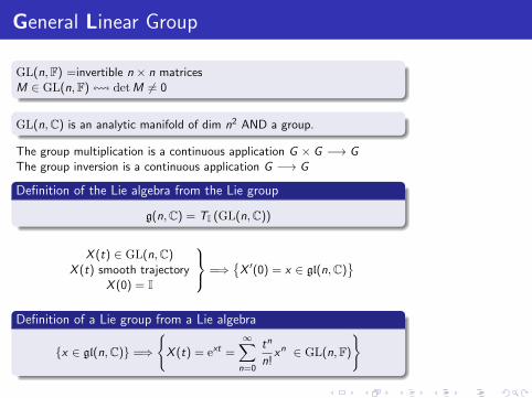
General Linear Group

GL(n,F) =invertible n × n matricesM ∈ GL(n,F)! detM 6= 0

GL(n,C) is an analytic manifold of dim n2 AND a group.

The group multiplication is a continuous application G × G −→ GThe group inversion is a continuous application G −→ G

Definition of the Lie algebra from the Lie group

g(n,C) = TI (GL(n,C))

X (t) ∈ GL(n,C)X (t) smooth trajectory

X (0) = I

=⇒{X ′(0) = x ∈ gl(n,C)

}

Definition of a Lie group from a Lie algebra

{x ∈ gl(n,C)} =⇒

{X (t) = ext =

∞∑n=0

tn

n!xn ∈ GL(n,F)

}

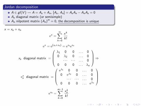
Jordan decomposition

A ∈ gl(V ) A = As + An, [As , An] = AsAn − AnAs = 0As diagonal matrix (or semisimple)An nilpotent matrix (An)m = 0, the decomposition is unique

x = xs + xn

ex =∞∑k=0

xk

k!

ex = e(xs+xn) = exsexn

xs diagonal matrix =

λ1 0 0 . . . 00 λ2 0 . . . 0· · · · · · . . . 0

0 0 0 . . . λn

⇒

exs diagonal matrix =

eλ1 0 0 . . . 00 eλ2 0 . . . 0· · · · · · . . . 0

0 0 0 . . . eλn

exn =

m−1∑k=0

xknk!

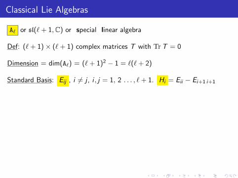
Classical Lie Algebras

A` or sl(`+ 1,C) or special linear algebra

Def: (`+ 1)× (`+ 1) complex matrices T with TrT = 0

Dimension = dim(A`) = (`+ 1)2 − 1 = `(`+ 2)

Standard Basis: Eij , i 6= j , i , j = 1, 2 . . . , `+ 1. Hi = Eii − Ei+1 i+1

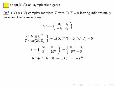
C` or sp(2`,C) or symplectic algebra

Def: (2`)× (2`) complex matrices T with TrT = 0 leaving infinitesimallyinvariant the bilinear form

b ←→(

0` I`−I` 0`

)U, V ∈ C2`

T ∈ sp(2`,C)

} b(U,TV ) + b(TU,V ) = 0

T =

(M NP −Mtr

)

{Ntr = N,Ptr = P

bT + T trb = 0 bTb−1 = −T tr

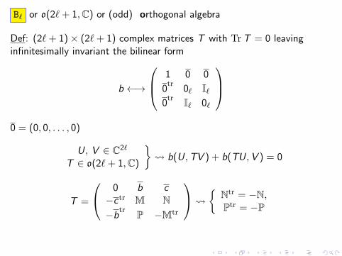
B` or o(2`+ 1,C) or (odd) orthogonal algebra

Def: (2`+ 1)× (2`+ 1) complex matrices T with TrT = 0 leavinginfinitesimally invariant the bilinear form

b ←→

1 0 0

0tr

0` I`0tr I` 0`

0 = (0, 0, . . . , 0)

U, V ∈ C2`

T ∈ o(2`+ 1,C)

} b(U,TV ) + b(TU,V ) = 0

T =

0 b c−ctr M N−btr P −Mtr

{Ntr = −N,Ptr = −P

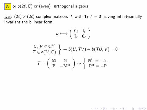
D` or o(2`,C) or (even) orthogonal algebra

Def: (2`)× (2`) complex matrices T with TrT = 0 leaving infinitesimallyinvariant the bilinear form

b ←→(

0` I`I` 0`

)U, V ∈ C2`

T ∈ o(2`,C)

} b(U,TV ) + b(TU,V ) = 0

T =

(M NP −Mtr

)

{Ntr = −N,Ptr = −P

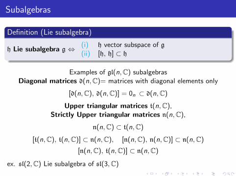
Subalgebras

Definition (Lie subalgebra)

h Lie subalgebra g ⇔ (i) h vector subspace of g(ii) [h, h] ⊂ h

Examples of gl(n,C) subalgebrasDiagonal matrices d(n,C)= matrices with diagonal elements only

[d(n,C), d(n,C)] = 0n ⊂ d(n,C)

Upper triangular matrices t(n,C),Strictly Upper triangular matrices n(n,C),

n(n,C) ⊂ t(n,C)

[t(n,C), t(n,C)] ⊂ n(n,C), [n(n,C), n(n,C)] ⊂ n(n,C)

[n(n,C), t(n,C)] ⊂ n(n,C)

ex. sl(2,C) Lie subalgebra of sl(3,C)

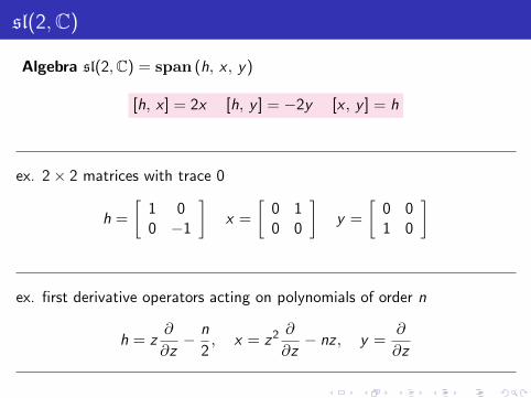
sl(2,C)

Algebra sl(2,C) = span (h, x , y)

[h, x ] = 2x [h, y ] = −2y [x , y ] = h

ex. 2× 2 matrices with trace 0

h =

[1 00 −1

]x =

[0 10 0

]y =

[0 01 0

]

ex. first derivative operators acting on polynomials of order n

h = z∂

∂z− n

2, x = z2 ∂

∂z− nz , y =

∂

∂z

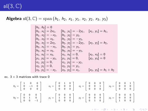
sl(3,C)

Algebra sl(3,C) = span (h1, h2, x1, y1, x2, y2, x3, y3)

[h1, h2] = 0[h1, x1] = 2x1, [h1, y1] = −2y1, [x1, y1] = h1,[h1, x2] = −x2, [h1, y2] = y2,[h1, x3] = x3, [h1, y3] = −y3,[h2, x2] = 2x2, [h2, y2] = −2y2, [x2, y2] = h2,[h2, x1] = −x1, [h2, y1] = y1,[h2, x3] = x3, [h2, y3] = −y3,[x1, x2] = x3, [x1, x3] = 0, [x2, x3] = 0[y1, y2] = −y3, [y1, y3] = 0, [y2, y3] = 0[x1, y2] = 0, [x1, y3] = −y2,[x2, y1] = 0, [x2, y3] = y1,[x3, y1] = −x2, [x3, y2] = x1, [x3, y3] = h1 + h2

ex. 3× 3 matrices with trace 0

h1 =

1 0 00 −1 00 0 0

h2 =

0 0 00 1 00 0 −1

x1 =

0 1 00 0 00 0 0

x2 =

0 0 00 0 10 0 0

x3 =

0 0 10 0 00 0 0

y1 =

0 0 01 0 00 0 0

y2 =

0 0 00 0 00 1 0

y3 =

0 0 00 0 01 0 0

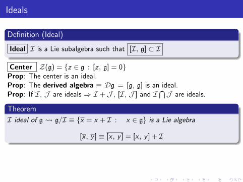
Ideals

Definition (Ideal)

Ideal I is a Lie subalgebra such that [I, g] ⊂ I

Center Z(g) = {z ∈ g : [z , g] = 0}Prop: The center is an ideal.Prop: The derived algebra ≡ Dg = [g, g] is an ideal.Prop: If I, J are ideals ⇒ I + J , [I, J ] and I

⋂J are ideals.

Theorem

I ideal of g g/I ≡ {x = x + I : x ∈ g} is a Lie algebra

[x , y ] ≡ [x , y ] = [x , y ] + I

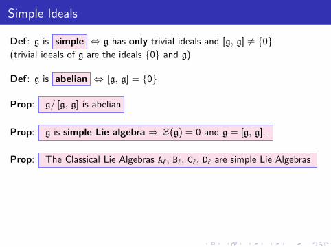
Simple Ideals

Def: g is simple ⇔ g has only trivial ideals and [g, g] 6= {0}(trivial ideals of g are the ideals {0} and g)

Def: g is abelian ⇔ [g, g] = {0}

Prop: g/ [g, g] is abelian

Prop: g is simple Lie algebra ⇒ Z(g) = 0 and g = [g, g].

Prop: The Classical Lie Algebras A`, B`, C`, D` are simple Lie Algebras

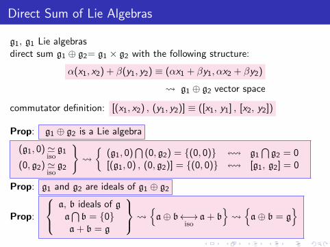
Direct Sum of Lie Algebras

g1, g1 Lie algebrasdirect sum g1 ⊕ g2= g1 × g2 with the following structure:

α(x1, x2) + β(y1, y2) ≡ (αx1 + βy1, αx2 + βy2)

g1 ⊕ g2 vector space

commutator definition: [(x1, x2) , (y1, y2)] ≡ ([x1, y1] , [x2, y2])

Prop: g1 ⊕ g2 is a Lie algebra

(g1, 0)'iso

g1

(0, g2)'iso

g2

}

{(g1, 0)

⋂(0, g2) = {(0, 0)} ! g1

⋂g2 = 0

[(g1, 0) , (0, g2)] = {(0, 0)} ! [g1, g2] = 0

Prop: g1 and g2 are ideals of g1 ⊕ g2

Prop:

a, b ideals of ga⋂b = {0}

a + b = g

{a⊕ b←→

isoa + b

} {a⊕ b = g

}

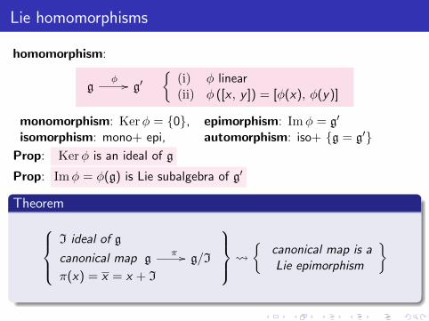
Lie homomorphisms

homomorphism:

gφ // g′

{(i) φ linear(ii) φ ([x , y ]) = [φ(x), φ(y)]

monomorphism: Kerφ = {0}, epimorphism: Imφ = g′

isomorphism: mono+ epi, automorphism: iso+ {g = g′}Prop: Kerφ is an ideal of g

Prop: Imφ = φ(g) is Lie subalgebra of g′

TheoremI ideal of g

canonical map gπ // g/I

π(x) = x = x + I

{

canonical map is aLie epimorphism

}

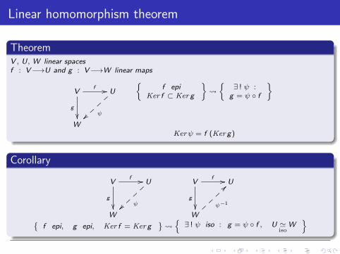
Linear homomorphism theorem

TheoremV , U, W linear spacesf : V−→U and g : V−→W linear maps

Vf //

g

��

U

ψ~~W

{f epi

Ker f ⊂ Ker g

}

{∃ ! ψ :

g = ψ ◦ f

}

Kerψ = f (Ker g)

Corollary

Vf //

g

��

U

ψ~~W

Vf //

g

��

U>>

ψ−1

W{f epi, g epi, Ker f = Ker g

} {∃ ! ψ iso : g = ψ ◦ f , U '

isoW

}

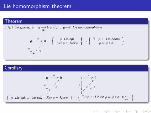
Lie homomorphism theorem

Theoremg, h, l Lie spaces, φ : g−→

epih and ρ : g−→l Lie homomorphisms

gφ //

ρ

��

h

ψ��

l

{φ Lie-epi,

Kerφ ⊂ Ker ρ

}

{∃ ! ψ : Lie-homo

ρ = ψ ◦ φ

}

Corollary

gφ //

ρ

��

h

ψ��

l

gφ //

ρ

��

h@@

ψ−1

l{φ Lie-epi, ρ Lie-epi, Kerφ = Ker ρ

} {∃ !ψ : Lie-iso ρ = ψ ◦ φ, h '

isol}

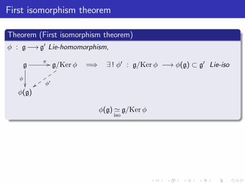
First isomorphism theorem

Theorem (First isomorphism theorem)

φ : g−→ g′ Lie-homomorphism,

gπ //

φ��

g/Kerφ

φ′zzφ(g)

=⇒ ∃ ! φ′ : g/Kerφ −→ φ(g) ⊂ g′ Lie-iso

φ(g)'iso

g/Kerφ

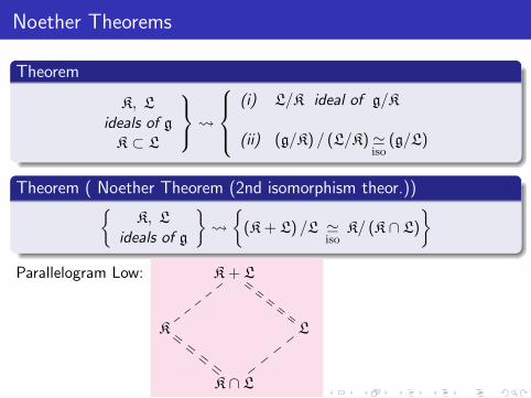
Noether Theorems

Theorem

K, Lideals of gK ⊂ L

(i) L/K ideal of g/K

(ii) (g/K) / (L/K)'iso

(g/L)

Theorem ( Noether Theorem (2nd isomorphism theor.)){K, L

ideals of g

}

{(K + L) /L '

isoK/ (K ∩ L)

}Parallelogram Low: K + L

K L

K ∩ L

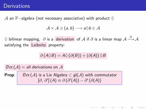
Derivations

A an F−algebra (not necessary associative) with product ♦

A×A 3 (a, b) −→ a♦b ∈ A

♦ bilinear mapping, ∂ is a derivation of A if ∂ is a linear map A ∂−→Asatisfying the Leibnitz property:

∂ (A♦B) = A♦ (∂(B)) + (∂(A))♦B

Der (A) = all derivations on A

Prop: Der (A) is a Lie Algebra ⊂ gl(A) with commutator[∂, ∂′] (A) ≡ ∂ (∂′(A))− ∂′ (∂(A))

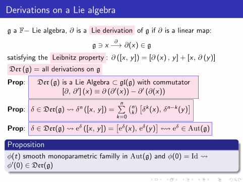
Derivations on a Lie algebra

g a F− Lie algebra, ∂ is a Lie derivation of g if ∂ is a linear map:

g 3 x∂−→ ∂(x) ∈ g

satisfying the Leibnitz property : ∂ ([x , y ]) = [∂ (x) , y ] + [x , ∂ (y)]

Der (g) = all derivations on g

Prop: Der (g) is a Lie Algebra ⊂ gl(g) with commutator[∂, ∂′] (x) ≡ ∂ (∂′(x))− ∂′ (∂(x))

Prop: δ ∈ Der(g) δn ([x , y ]) =n∑

k=0

(nk

) [δk(x), δn−k(y)

]Prop: δ ∈ Der(g) eδ ([x , y ]) =

[eδ(x), eδ(y)

]! eδ ∈ Aut(g)

Proposition

φ(t) smooth monoparametric familly in Aut(g) and φ(0) = Id φ′(0) ∈ Der(g)

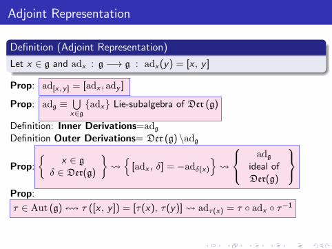
Adjoint Representation

Definition (Adjoint Representation)

Let x ∈ g and adx : g −→ g : adx(y) = [x , y ]

Prop: ad[x , y ] = [adx , ady ]

Prop: adg ≡⋃x∈g{adx} Lie-subalgebra of Der (g)

Definition: Inner Derivations=adgDefinition Outer Derivations= Der (g) \adg

Prop:

{x ∈ g

δ ∈ Der(g)

} {

[adx , δ] = −adδ(x)

}

adg

ideal ofDer(g)

Prop:

τ ∈ Aut (g)! τ ([x , y ]) = [τ(x), τ(y)] adτ(x) = τ ◦ adx ◦ τ−1

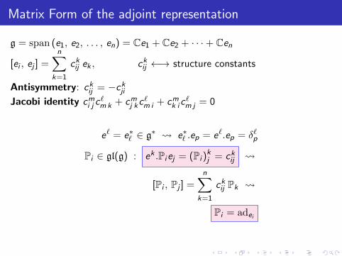
Matrix Form of the adjoint representation

g = span (e1, e2, . . . , en) = Ce1 + Ce2 + · · ·+ Cen

[ei , ej ] =n∑

k=1

ckij ek , ckij ←→ structure constants

Antisymmetry: ckij = −ckjiJacobi identity cmi j c

`mk + cmj kc

`m i + cmk ic

`m j = 0

e` = e∗` ∈ g∗ e∗` .ep = e`.ep = δ`p

Pi ∈ gl(g) : ek .Piej = (Pi )kj = ckij

[Pi , Pj ] =n∑

k=1

ckij Pk

Pi = adei

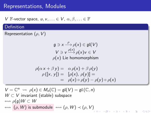
Representations, Modules

V F-vector space, u, v , . . . ∈ V , α, β, . . . ∈ F

Definition

Representation (ρ,V )

g 3 xρ−→ ρ(x) ∈ gl(V )

V 3 vρ(x)−→ ρ(x)v ∈ V

ρ(x) Lie homomorphism

ρ(α x + β y) = αρ(x) + β ρ(y)ρ ([x , y ]) = [ρ(x), ρ(y)] =

= ρ(x) ◦ ρ(y)− ρ(y) ◦ ρ(x)

V = Cn ρ(x) ∈ Mn(C) = gl(V ) = gl (C, n)W ⊂ V invariant (stable) subspace! ρ(g)W ⊂W

! (ρ,W ) is submodule ! (ρ,W ) ≺ (ρ,V )

1.pdf

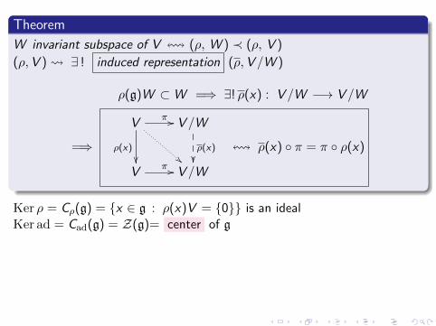
Theorem

W invariant subspace of V ! (ρ, W ) ≺ (ρ, V )

(ρ,V ) ∃ ! induced representation (ρ,V /W )

ρ(g)W ⊂W =⇒ ∃! ρ(x) : V /W −→ V /W

=⇒

V

ρ(x)

��

π //

!!

V /W

ρ(x)��

Vπ // V /W

! ρ(x) ◦ π = π ◦ ρ(x)

Ker ρ = Cρ(g) = {x ∈ g : ρ(x)V = {0}} is an idealKer ad = Cad(g) = Z(g)= center of g

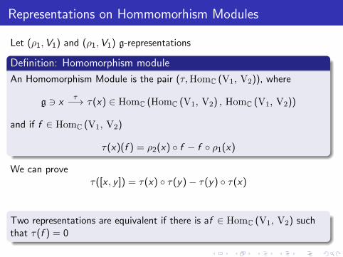
Representations on Hommomorhism Modules

Let (ρ1,V1) and (ρ1,V1) g-representations

Definition: Homomorphism module

An Homomorphism Module is the pair (τ,HomC (V1, V2)), where

g 3 xτ−→ τ(x) ∈ HomC (HomC (V1, V2) , HomC (V1, V2))

and if f ∈ HomC (V1, V2)

τ(x)(f ) = ρ2(x) ◦ f − f ◦ ρ1(x)

We can proveτ([x , y ]) = τ(x) ◦ τ(y)− τ(y) ◦ τ(x)

Two representations are equivalent if there is af ∈ HomC (V1, V2) suchthat τ(f ) = 0

Reducible and Irreducible representation

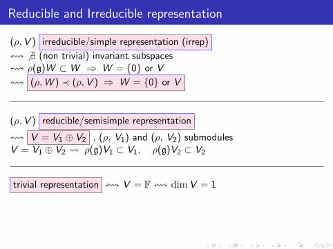
(ρ,V ) irreducible/simple representation (irrep)

! 6 ∃ (non trivial) invariant subspaces! ρ(g)W ⊂W ⇒ W = {0} or V

! (ρ,W ) ≺ (ρ,V ) ⇒ W = {0} or V

(ρ,V ) reducible/semisimple representation

! V = V1 ⊕ V2 , (ρ, V1) and (ρ, V2) submodulesV = V1 ⊕ V2 ρ(g)V1 ⊂ V1, ρ(g)V2 ⊂ V2

trivial representation ! V = F! dimV = 1

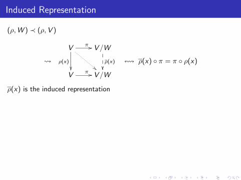
Induced Representation

(ρ,W ) ≺ (ρ,V )

V

ρ(x)

��

π //

!!

V /W

ρ(x)��

Vπ // V /W

! ρ(x) ◦ π = π ◦ ρ(x)

ρ(x) is the induced representation

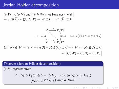
Jordan Holder decomposition

(ρ,W ) ≺ (ρ,V ) and (ρ,V /W ) not irrep nor trivial

∃(ρ,U

)≺ (ρ,V /W ) W ⊂ U = π−1(U) ⊂ V

V

ρ(x)

��

π //

!!

V /W

ρ(x)��

Vπ // V /W

! ρ(x) ◦ π = π ◦ ρ(x)

(π ◦ ρ(x)) (U) = (ρ(x) ◦ π) (U) = ρ(x)(U)⊂ U = π(U) ρ(x)(U) ⊂ U

(ρ,W ) ≺ (ρ,U) ≺ (ρ,V )

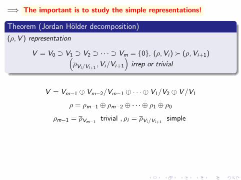
Theorem (Jordan Holder decomposition)

(ρ,V ) representation

V = V0 ⊃ V1 ⊃ V2 ⊃ · · · ⊃ Vm = {0}, (ρ,Vi ) � (ρ,Vi+1)(ρVi/Vi+1

,Vi/Vi+1

)irrep or trivial

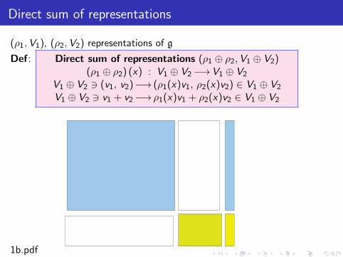
Direct sum of representations

(ρ1,V1), (ρ2,V2) representations of g

Def: Direct sum of representations (ρ1 ⊕ ρ2,V1 ⊕ V2)(ρ1 ⊕ ρ2) (x) : V1 ⊕ V2−→V1 ⊕ V2

V1 ⊕ V2 3 (v1, v2)−→ (ρ1(x)v1, ρ2(x)v2) ∈ V1 ⊕ V2

V1 ⊕ V2 3 v1 + v2−→ ρ1(x)v1 + ρ2(x)v2 ∈ V1 ⊕ V2

1b.pdf

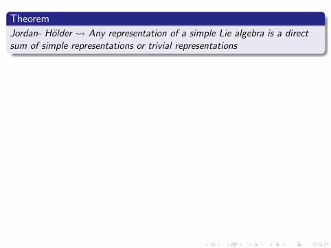
Theorem

Jordan- Holder Any representation of a simple Lie algebra is a directsum of simple representations or trivial representations

=⇒ The important is to study the simple representations!

Theorem (Jordan Holder decomposition)

(ρ,V ) representation

V = V0 ⊃ V1 ⊃ V2 ⊃ · · · ⊃ Vm = {0}, (ρ,Vi ) � (ρ,Vi+1)(ρVi/Vi+1

,Vi/Vi+1

)irrep or trivial

V = Vm−1 ⊕ Vm−2/Vm−1 ⊕ · · · ⊕ V1/V2 ⊕ V /V1

ρ = ρm−1 ⊕ ρm−2 ⊕ · · · ⊕ ρ1 ⊕ ρ0

ρm−1 = ρVm−1trivial , ρi = ρVi/Vi+1

simple

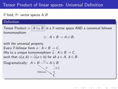
Tensor Product of linear spaces- Universal Definition

F field, F– vector spaces A,B

Definition

Tensor Product ≡ A⊗F B is a F-vector space AND a canonical bilinearhomomorphism

⊗ : A× B → A⊗ B,

with the universal property.Every F-bilinear form φ : A× B → C ,lifts to a unique homomorphism φ : A⊗ B → C ,such that φ(a, b) = φ(a⊗ b) for all a ∈ A, b ∈ B.

Diagramatically: A× Bφ

bilinear %%

⊗ // A⊗ B

∃! φ

��C

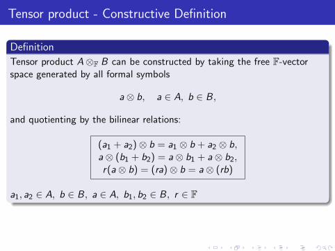
Tensor product - Constructive Definition

Definition

Tensor product A⊗F B can be constructed by taking the free F-vectorspace generated by all formal symbols

a⊗ b, a ∈ A, b ∈ B,

and quotienting by the bilinear relations:

(a1 + a2)⊗ b = a1 ⊗ b + a2 ⊗ b,a⊗ (b1 + b2) = a⊗ b1 + a⊗ b2,r(a⊗ b) = (ra)⊗ b = a⊗ (rb)

a1, a2 ∈ A, b ∈ B, a ∈ A, b1, b2 ∈ B, r ∈ F

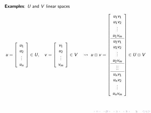
Examples: U and V linear spaces

u =

u1

u2...un

∈ U, v =

v1

u2...vm

∈ V u ⊗ v =

u1v1

u1v2...

u1vmu2v1

u2v2...

u2vm......

unv1

unv2...

unvm

∈ U ⊗ V

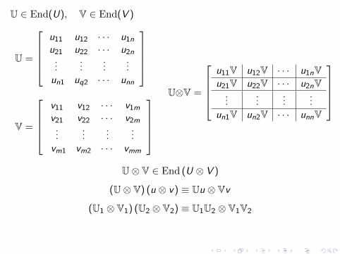
U ∈ End(U), V ∈ End(V )

U =

u11 u12 · · · u1n

u21 u22 · · · u2n...

......

...un1 uq2 · · · unn

V =

v11 v12 · · · v1m

v21 v22 · · · v2m...

......

...vm1 vm2 · · · vmm

U⊗V =

u11V u12V · · · u1nVu21V u22V · · · u2nV

......

......

un1V un2V · · · unnV

U⊗ V ∈ End (U ⊗ V )

(U⊗ V) (u ⊗ v) ≡ Uu ⊗ Vv

(U1 ⊗ V1) (U2 ⊗ V2) ≡ U1U2 ⊗ V1V2

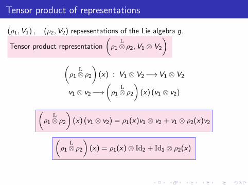
Tensor product of representations

(ρ1,V1) , (ρ2,V2) repsesentations of the Lie algebra g.

Tensor product representation

(ρ1

L⊗ ρ2,V1 ⊗ V2

)(ρ1

L⊗ ρ2

)(x) : V1 ⊗ V2−→V1 ⊗ V2

v1 ⊗ v2−→(ρ1

L⊗ ρ2

)(x) (v1 ⊗ v2)

(ρ1

L⊗ ρ2

)(x) (v1 ⊗ v2) = ρ1(x)v1 ⊗ v2 + v1 ⊗ ρ2(x)v2

(ρ1

L⊗ ρ2

)(x) = ρ1(x)⊗ Id2 + Id1 ⊗ ρ2(x)

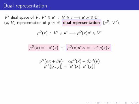
Dual representation

V ∗ dual space of V , V ∗ 3 u∗ : V 3 v −→ u∗.v ∈ C(ρ, V ) representation of g ∃! dual representation

(ρD , V ∗

)ρD(x) : V ∗ 3 u∗ −→ ρD(x)u∗ ∈ V ∗

ρD(x) = −ρ∗(x) ρD(x)u∗.v = −u∗.ρ(x)v

ρD(αx + βy) = αρD(x) + βρD(y)ρD ([x , y ]) =

[ρD(x), ρD(y)

]

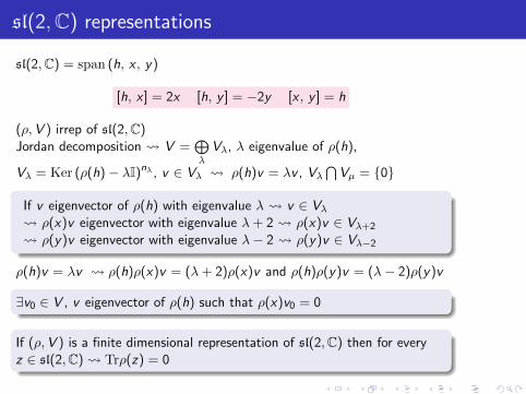
sl(2,C) representations

sl(2,C) = span (h, x , y)

[h, x ] = 2x [h, y ] = −2y [x , y ] = h

(ρ,V ) irrep of sl(2,C)Jordan decomposition V =

⊕λ

Vλ, λ eigenvalue of ρ(h),

Vλ = Ker (ρ(h)− λI)nλ , v ∈ Vλ ρ(h)v = λv , Vλ⋂Vµ = {0}

If v eigenvector of ρ(h) with eigenvalue λ v ∈ Vλ ρ(x)v eigenvector with eigenvalue λ+ 2 ρ(x)v ∈ Vλ+2

ρ(y)v eigenvector with eigenvalue λ− 2 ρ(y)v ∈ Vλ−2

ρ(h)v = λv ρ(h)ρ(x)v = (λ+ 2)ρ(x)v and ρ(h)ρ(y)v = (λ− 2)ρ(y)v

∃v0 ∈ V , v eigenvector of ρ(h) such that ρ(x)v0 = 0

If (ρ,V ) is a finite dimensional representation of sl(2,C) then for everyz ∈ sl(2,C) Trρ(z) = 0

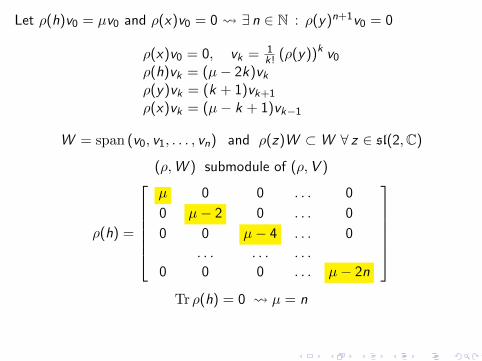
Let ρ(h)v0 = µv0 and ρ(x)v0 = 0 ∃ n ∈ N : ρ(y)n+1v0 = 0

ρ(x)v0 = 0, vk = 1k! (ρ(y))k v0

ρ(h)vk = (µ− 2k)vkρ(y)vk = (k + 1)vk+1

ρ(x)vk = (µ− k + 1)vk−1

W = span (v0, v1, . . . , vn) and ρ(z)W ⊂W ∀ z ∈ sl(2,C)

(ρ,W ) submodule of (ρ,V )

ρ(h) =

µ 0 0 . . . 0

0 µ− 2 0 . . . 0

0 0 µ− 4 . . . 0

. . . . . . . . .

0 0 0 . . . µ− 2n

Tr ρ(h) = 0 µ = n

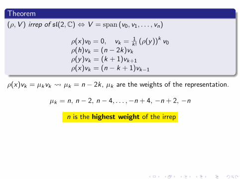
Theorem

(ρ,V ) irrep of sl(2,C) ⇔ V = span (v0, v1, . . . , vn)

ρ(x)v0 = 0, vk = 1k! (ρ(y))k v0

ρ(h)vk = (n − 2k)vkρ(y)vk = (k + 1)vk+1

ρ(x)vk = (n − k + 1)vk−1

ρ(x)vk = µkvk µk = n − 2k, µk are the weights of the representation.

µk = n, n − 2, n − 4, . . . ,−n + 4, −n + 2, −n

n is the highest weight of the irrep

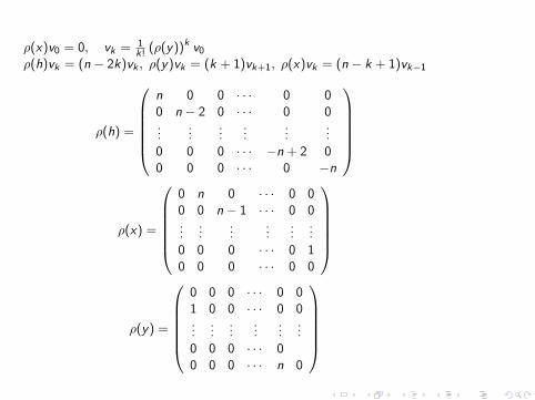
ρ(x)v0 = 0, vk = 1k! (ρ(y))k v0

ρ(h)vk = (n − 2k)vk , ρ(y)vk = (k + 1)vk+1, ρ(x)vk = (n − k + 1)vk−1

ρ(h) =

n 0 0 · · · 0 00 n − 2 0 · · · 0 0...

......

......

...0 0 0 · · · −n + 2 00 0 0 · · · 0 −n

ρ(x) =

0 n 0 · · · 0 00 0 n − 1 · · · 0 0...

......

......

...0 0 0 · · · 0 10 0 0 · · · 0 0

ρ(y) =

0 0 0 · · · 0 01 0 0 · · · 0 0...

......

......

...0 0 0 · · · 00 0 0 · · · n 0

dimV = n + 1Eigenvalues

−n, −n + 2, . . . , n − 2, n

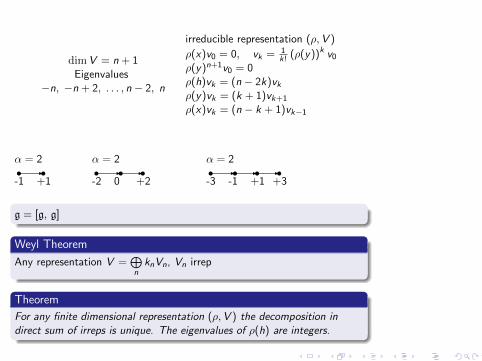
irreducible representation (ρ,V )

ρ(x)v0 = 0, vk = 1k! (ρ(y))k v0

ρ(y)n+1v0 = 0ρ(h)vk = (n − 2k)vkρ(y)vk = (k + 1)vk+1

ρ(x)vk = (n − k + 1)vk−1

α = 2s -s-1 +1

α = 2s -s -s-2 0 +2

α = 2s -s -s -s-3 -1 +1 +3

g = [g, g]

Weyl Theorem

Any representation V =⊕nknVn, Vn irrep

Theorem

For any finite dimensional representation (ρ,V ) the decomposition indirect sum of irreps is unique. The eigenvalues of ρ(h) are integers.

Weyl Theorem sl(2)

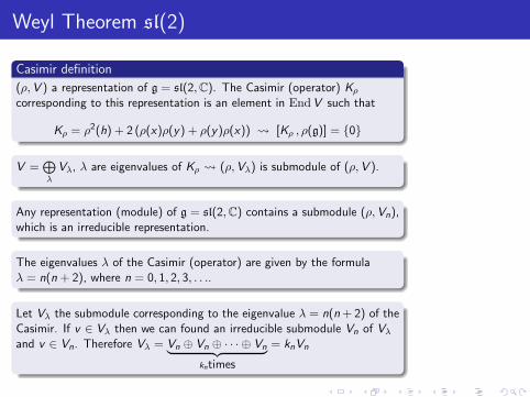
Casimir definition

(ρ,V ) a representation of g = sl(2,C). The Casimir (operator) Kρcorresponding to this representation is an element in EndV such that

Kρ = ρ2(h) + 2 (ρ(x)ρ(y) + ρ(y)ρ(x)) [Kρ , ρ(g)] = {0}

V =⊕λ

Vλ, λ are eigenvalues of Kρ (ρ,Vλ) is submodule of (ρ,V ).

Any representation (module) of g = sl(2,C) contains a submodule (ρ,Vn),which is an irreducible representation.

The eigenvalues λ of the Casimir (operator) are given by the formulaλ = n(n + 2), where n = 0, 1, 2, 3, . . ..

Let Vλ the submodule corresponding to the eigenvalue λ = n(n + 2) of theCasimir. If v ∈ Vλ then we can found an irreducible submodule Vn of Vλand v ∈ Vn. Therefore Vλ = Vn ⊕ Vn ⊕ · · · ⊕ Vn︸ ︷︷ ︸

kntimes

= knVn

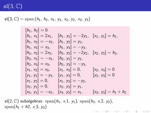
sl(3,C)

sl(3,C) = span (h1, h2, x1, y1, x2, y2, x3, y3)

[h1, h2] = 0[h1, x1] = 2x1, [h1, y1] = −2y1, [x1, y1] = h1,[h1, x2] = −x2, [h1, y2] = y2,[h1, x3] = x3, [h1, y3] = −y3,[h2, x2] = 2x2, [h2, y2] = −2y2, [x2, y2] = h2,[h2, x1] = −x1, [h2, y1] = y1,[h2, x3] = x3, [h2, y3] = −y3,[x1, x2] = x3, [x1, x3] = 0, [x2, x3] = 0[y1, y2] = −y3, [y1, y3] = 0, [y2, y3] = 0[x1, y2] = 0, [x1, y3] = −y2,[x2, y1] = 0, [x2, y3] = y1,[x3, y1] = −x2, [x3, y2] = x1, [x3, y3] = h1 + h2

sl(2,C) subalgebras: span(h1, x,1, y1), span(h2, x,2, y2),span(h1 + h2, x,3, y3)

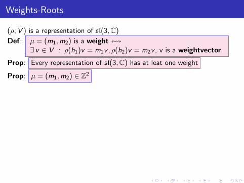
Weights-Roots

(ρ,V ) is a representation of sl(3,C)

Def: µ = (m1,m2) is a weight!∃ v ∈ V : ρ(h1)v = m1v , ρ(h2)v = m2v , v is a weightvector

Prop: Every representation of sl(3,C) has at leat one weight

Prop: µ = (m1,m2) ∈ Z2

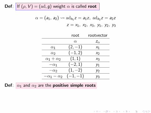
Def: If (ρ,V ) = (ad, g) weight α is called root

α = (a1, a2) adh1z = a1z , adh2z = a2z

z = x1, x2, x3, y1, y2, y3

root rootvector

α zαα1 (2,−1) x1

α2 (−1, 2) x2

α1 + α2 (1, 1) x3

−α1 (−2, 1) y1

−α2 (1,−2) y2

−α1 − α2 (−1,−1) y3

Def: α1 and α2 are the positive simple roots

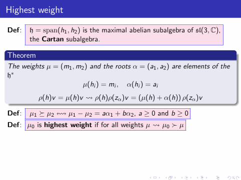
Highest weight

Def: h = span(h1, h2) is the maximal abelian subalgebra of sl(3,C),the Cartan subalgebra.

Theorem

The weights µ = (m1,m2) and the roots α = (a1, a2) are elements of theh∗

µ(hi ) = mi , α(hi ) = ai

ρ(h)v = µ(h)v ρ(h)ρ(zα)v = (µ(h) + α(h)) ρ(zα)v

Def: µ1 � µ2 ! µ1 − µ2 = aα1 + bα2, a ≥ 0 and b ≥ 0

Def: µ0 is highest weight if for all weights µ µ0 � µ

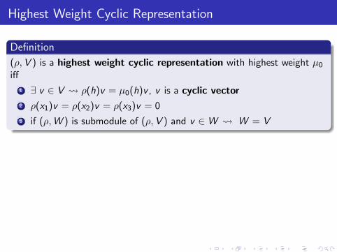
Highest Weight Cyclic Representation

Definition

(ρ,V ) is a highest weight cyclic representation with highest weight µ0

iff

1 ∃ v ∈ V ρ(h)v = µ0(h)v , v is a cyclic vector

2 ρ(x1)v = ρ(x2)v = ρ(x3)v = 0

3 if (ρ,W ) is submodule of (ρ,V ) and v ∈W W = V

Theorem

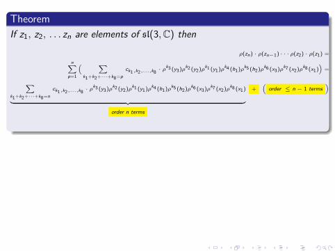
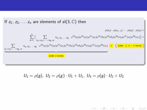
If z1, z2, . . . zn are elements of sl(3,C) then

ρ(zn) · ρ(zn−1) · · · ρ(z2) · ρ(z1) =

n∑p=1

( ∑k1+k2+···+k8=p

ck1,k2,...,k8· ρk3 (y3)ρk2 (y2)ρk1 (y1)ρk4 (h1)ρk5 (h2)ρk6 (x3)ρk7 (x2)ρk8 (x1)

)=

∑k1+k2+···+k8=n

ck1,k2,...,k8· ρk3 (y3)ρk2 (y2)ρk1 (y1)ρk4 (h1)ρk5 (h2)ρk6 (x3)ρk7 (x2)ρk8 (x1)

︸ ︷︷ ︸order n terms

+(

order ≤ n − 1 terms)

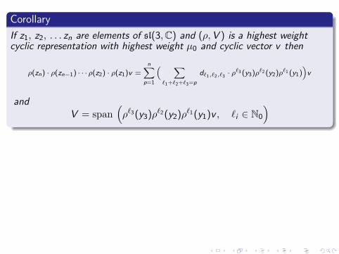
Corollary

If z1, z2, . . . zn are elements of sl(3,C) and (ρ,V ) is a highest weightcyclic representation with highest weight µ0 and cyclic vector v then

ρ(zn) · ρ(zn−1) · · · ρ(z2) · ρ(z1)v =n∑

p=1

( ∑`1+`2+`3=p

d`1,`2,`3· ρ`3 (y3)ρ`2 (y2)ρ`1 (y1)

)v

andV = span

(ρ`3(y3)ρ`2(y2)ρ`1(y1)v , `i ∈ N0

)

If z1, z2, . . . zn are elements of sl(3,C) then

ρ(zn) · ρ(zn−1) · · · ρ(z2) · ρ(z1) =

n∑p=1

( ∑k1+k2+···+k8=p

ck1,k2,...,k8· ρk3 (y3)ρk2 (y2)ρk1 (y1)ρk4 (h1)ρk5 (h2)ρk6 (x3)ρk7 (x2)ρk8 (x1)

)=

∑k1+k2+···+k8=n

ck1,k2,...,k8· ρk3 (y3)ρk2 (y2)ρk1 (y1)ρk4 (h1)ρk5 (h2)ρk6 (x3)ρk7 (x2)ρk8 (x1)

︸ ︷︷ ︸order n terms

+(

order ≤ n − 1 terms)

U1 = ρ(g), U2 = ρ(g) · U1 + U1, U3 = ρ(g) · U2 + U2

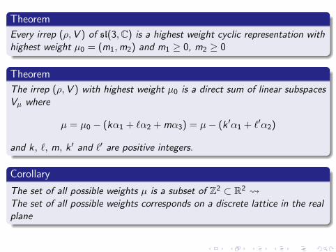
Theorem

Every irrep (ρ,V ) of sl(3,C) is a highest weight cyclic representation withhighest weight µ0 = (m1,m2) and m1 ≥ 0, m2 ≥ 0

Theorem

The irrep (ρ,V ) with highest weight µ0 is a direct sum of linear subspacesVµ where

µ = µ0 − (kα1 + `α2 + mα3) = µ− (k ′α1 + `′α2)

and k, `, m, k ′ and `′ are positive integers.

Corollary

The set of all possible weights µ is a subset of Z2 ⊂ R2 The set of all possible weights corresponds on a discrete lattice in the realplane

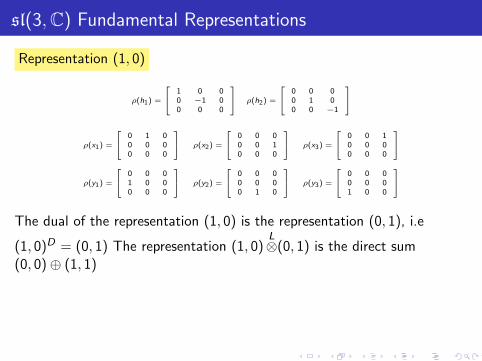
sl(3,C) Fundamental Representations

Representation (1, 0)

ρ(h1) =

1 0 00 −1 00 0 0

ρ(h2) =

0 0 00 1 00 0 −1

ρ(x1) =

0 1 00 0 00 0 0

ρ(x2) =

0 0 00 0 10 0 0

ρ(x3) =

0 0 10 0 00 0 0

ρ(y1) =

0 0 01 0 00 0 0

ρ(y2) =

0 0 00 0 00 1 0

ρ(y3) =

0 0 00 0 01 0 0

The dual of the representation (1, 0) is the representation (0, 1), i.e

(1, 0)D = (0, 1) The representation (1, 0)L⊗(0, 1) is the direct sum

(0, 0)⊕ (1, 1)

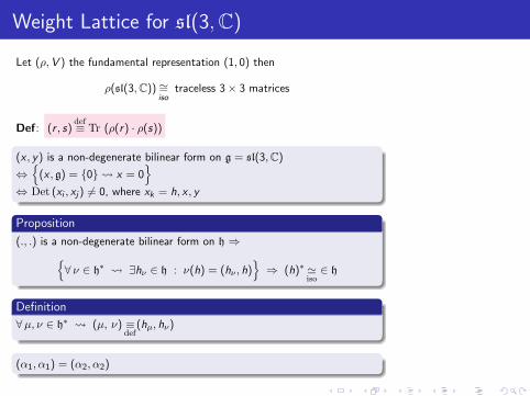
Weight Lattice for sl(3,C)

Let (ρ,V ) the fundamental representation (1, 0) then

ρ(sl(3,C)) ∼=iso

traceless 3× 3 matrices

Def: (r , s)def≡ Tr (ρ(r) · ρ(s))

(x , y) is a non-degenerate bilinear form on g = sl(3,C)

⇔{

(x , g) = {0} x = 0}

⇔ Det (xi , xj) 6= 0, where xk = h, x , y

Proposition

(., .) is a non-degenerate bilinear form on h ⇒{∀ ν ∈ h∗ ∃hν ∈ h : ν(h) = (hν , h)

}⇒ (h)∗ '

iso∈ h

Definition

∀µ, ν ∈ h∗ (µ, ν) ≡def

(hµ, hν)

(α1, α1) = (α2, α2)

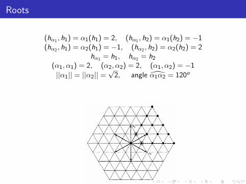
Roots

(hα1 , h1) = α1(h1) = 2, (hα1 , h2) = α1(h2) = −1(hα2 , h1) = α2(h1) = −1, (hα2 , h2) = α2(h2) = 2

hα1 = h1, hα2 = h2

(α1, α1) = 2, (α2, α2) = 2, (α1, α2) = −1

||α1|| = ||α2|| =√

2, angle α1α2 = 120o

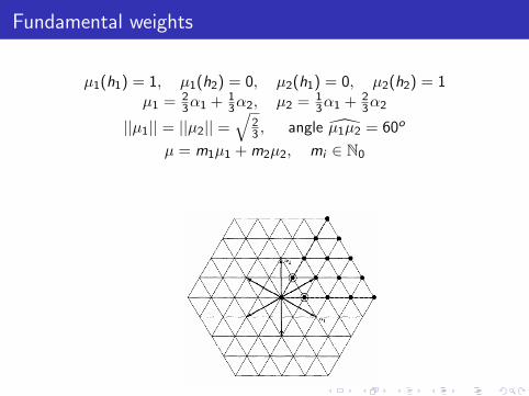
Fundamental weights

µ1(h1) = 1, µ1(h2) = 0, µ2(h1) = 0, µ2(h2) = 1µ1 = 2

3α1 + 13α2, µ2 = 1

3α1 + 23α2

||µ1|| = ||µ2|| =√

23 , angle µ1µ2 = 60o

µ = m1µ1 + m2µ2, mi ∈ N0

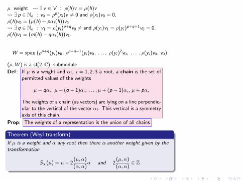
µ weight ∃ v ∈ V : ρ(h)v = µ(h)v ∃ p ∈ No : v0 = ρp(xi )v 6= 0 and ρ(xi )v0 = 0,ρ(h)v0 = (µ(h) + pαi (h))v0

∃ q ∈ No : v1 = ρ(yi )p+qv0 6= and ρ(yi )v1 = ρ(yi )

p+q+1v0 = 0,ρ(h)v1 = (m(h)− qαi (h))v1.

W = span(ρp+q(yi )v0, ρ

p+q−1(yi )v0, . . . , ρ(yi )2v0, . . . , ρ(yi )v0, v0

)(ρ,W ) is a sl(2,C) submodule

Def: If µ is a weight and αi , i = 1, 2, 3 a root, a chain is the set ofpermitted values of the weights

µ− qαi , µ− (q − 1)αi , . . . , µ+ (p − 1)αi , µ+ pαi

The weights of a chain (as vectors) are lying on a line perpendic-ular to the vertical of the vector αi . This vertical is a symmetryaxis of this chain.

Prop: The weights of a representation is the union of all chains

Theorem (Weyl transform)

If µ is a weight and α any root then there is another weight given by thetransformation

Sα (µ) = µ− 2(µ, α)

(α, α)α and 2

(µ, α)

(α, α)∈ Z

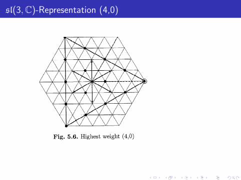
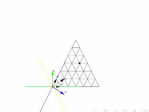
sl(3,C)-Representation (4,0)

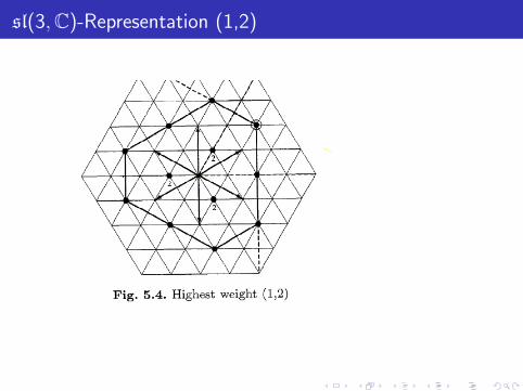
sl(3,C)-Representation (1,2)

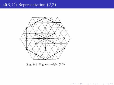
sl(3,C)-Representation (2,2)

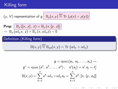
Killing form

(ρ, V ) representation of g Bρ(x , y)def≡ Tr (ρ(x) ◦ ρ(y))

Prop: Bρ ([x , y ] , z) = Bρ (x , [y , z ])

Bρ (adyx , z) + Bρ (x , adyz) = 0

Definition (Killing form)

B(x , y)def≡ Bad(x , y) = Tr (adx ◦ ady )

g = span (e1, e2, . . . , en)

g∗ = span(e1, e2, . . . , en

), e i (ej) = e i .ej = δij

B(x , y) =n∑

k=1

ek .adx ◦ adyek =n∑

k=1

ek . [x , [y , ek ]]

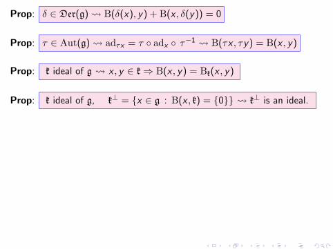
Prop: δ ∈ Der(g) B(δ(x), y) + B(x , δ(y)) = 0

Prop: τ ∈ Aut(g) adτx = τ ◦ adx ◦ τ−1 B(τx , τy) = B(x , y)

Prop: k ideal of g x , y ∈ k⇒ B(x , y) = Bk(x , y)

Prop: k ideal of g, k⊥ = {x ∈ g : B(x , k) = {0}} k⊥ is an ideal.

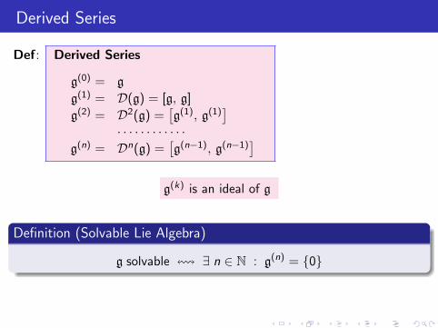
Derived Series

Def: Derived Series

g(0) = g

g(1) = D(g) = [g, g]

g(2) = D2(g) =[g(1), g(1)

]· · · · · · · · · · · ·

g(n) = Dn(g) =[g(n−1), g(n−1)

]g(k) is an ideal of g

Definition (Solvable Lie Algebra)

g solvable ! ∃ n ∈ N : g(n) = {0}

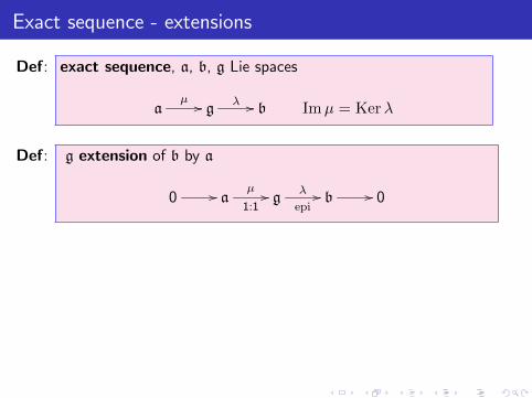
Exact sequence - extensions

Def: exact sequence, a, b, g Lie spaces

aµ // g

λ // b Imµ = Kerλ

Def: g extension of b by a

0 // aµ

1:1// g

λ

epi// b // 0

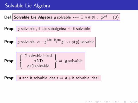
Solvable Lie Algebra

Def: Solvable Lie Algebra g solvable ! ∃ n ∈ N : g(n) = {0}

Prop: g solvable , k Lie-subalgebra k solvable

Prop: g solvable, φ : gLie−Hom−→ g′ φ(g) solvable

Prop:

I solvable ideal

ANDg/I solvable

⇒ g solvable

Prop: a and b solvable ideals ⇒ a + b solvable ideal

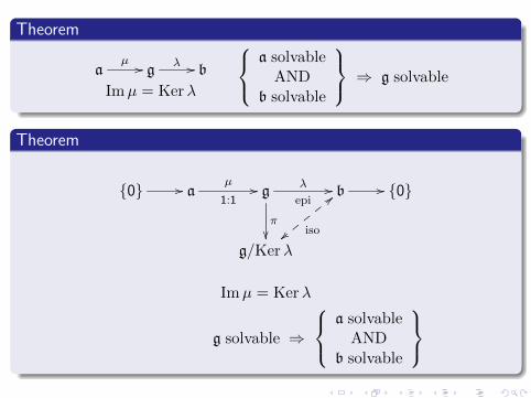
Theorem

aµ // g

λ // b

Imµ = Kerλ

a solvableAND

b solvable

⇒ g solvable

Theorem

{0} // aµ

1:1// g

λ

epi//

π

��

b // {0}

g/Kerλ|| iso

<<

Imµ = Kerλ

g solvable ⇒

a solvableAND

b solvable

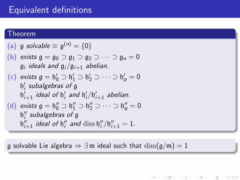
Equivalent definitions

Theorem

(a) g solvable ≡ g(n) = {0}(b) exists g = g0 ⊃ g1 ⊃ g2 ⊃ · · · ⊃ gn = 0

gi ideals and gi/gi+1 abelian.

(c) exists g = h′0 ⊃ h′1 ⊃ h′2 ⊃ · · · ⊃ h′p = 0h′i subalgebras of gh′i+1 ideal of h′i and h′i/h

′i+1 abelian.

(d) exists g = h′′0 ⊃ h′′1 ⊃ h′′2 ⊃ · · · ⊃ h′′q = 0h′′i subalgebras of gh′′i+1 ideal of h′′i and dim h′′i /h

′′i+1 = 1.

g solvable Lie algebra ⇒ ∃m ideal such that dim(g/m) = 1

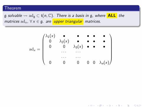
Theorem

g solvable adg ⊂ t(n,C). There is a basis in g, where ALL the

matrices adx , ∀ x ∈ g. are upper triangular matrices.

adx =

λ1(x) • • • • •0 λ2(x) • • • •0 0 λ3(x) • • •

· · · · · ·· · · · · ·

0 0 0 0 0 λn(x)

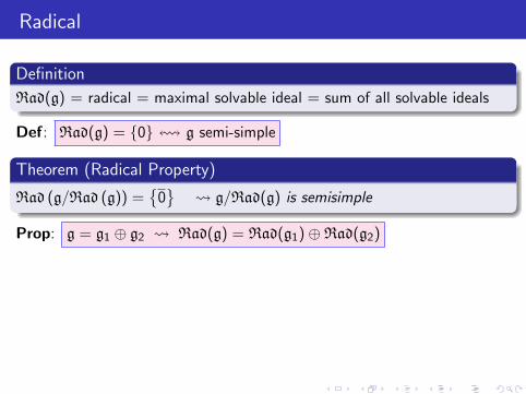
Radical

Definition

Rad(g) = radical = maximal solvable ideal = sum of all solvable ideals

Def: Rad(g) = {0}! g semi-simple

Theorem (Radical Property)

Rad (g/Rad (g)) ={

0} g/Rad(g) is semisimple

Prop: g = g1 ⊕ g2 Rad(g) = Rad(g1)⊕Rad(g2)

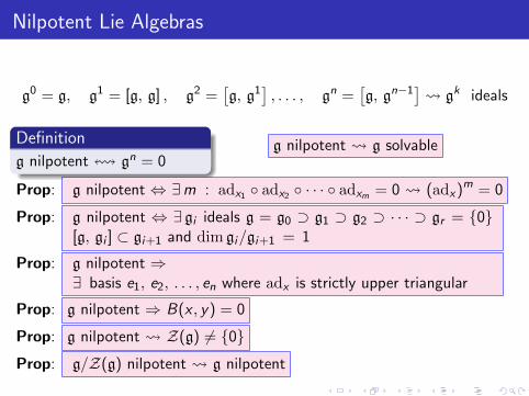
Nilpotent Lie Algebras

g0 = g, g1 = [g, g] , g2 =[g, g1

], . . . , gn =

[g, gn−1

] gk ideals

Definition

g nilpotent ! gn = 0g nilpotent g solvable

Prop: g nilpotent ⇔ ∃m : adx1 ◦ adx2 ◦ · · · ◦ adxm = 0 (adx)m = 0

Prop: g nilpotent ⇔ ∃ gi ideals g = g0 ⊃ g1 ⊃ g2 ⊃ · · · ⊃ gr = {0}[g, gi ] ⊂ gi+1 and dim gi/gi+1 = 1

Prop: g nilpotent ⇒∃ basis e1, e2, . . . , en where adx is strictly upper triangular

Prop: g nilpotent ⇒ B(x , y) = 0

Prop: g nilpotent Z(g) 6= {0}

Prop: g/Z(g) nilpotent g nilpotent

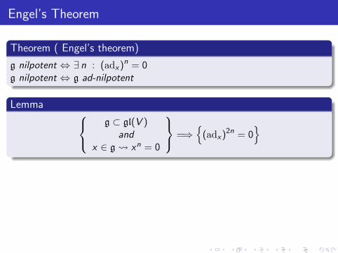
Engel’s Theorem

Theorem ( Engel’s theorem)

g nilpotent ⇔ ∃ n : (adx)n = 0g nilpotent ⇔ g ad-nilpotent

Lemma g ⊂ gl(V )

andx ∈ g xn = 0

=⇒{

(adx)2n = 0}

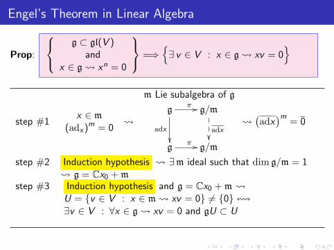
Engel’s Theorem in Linear Algebra

Prop:

g ⊂ gl(V )

andx ∈ g xn = 0

=⇒{∃ v ∈ V : x ∈ g xv = 0

}

step #1x ∈ m

(adx)m = 0

m Lie subalgebra of g

g

adx

��

π // g/m

adx��

gπ // g/m

(adx

)m= 0

step #2 Induction hypothesis ∃m ideal such that dim g/m = 1 g = Cx0 + m

step #3 Induction hypothesis and g = Cx0 + m U = {v ∈ V : x ∈ m xv = 0} 6= {0}!∃v ∈ V : ∀x ∈ g xv = 0 and gU ⊂ U

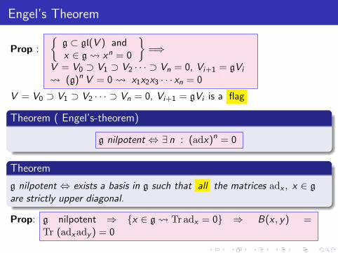
Engel’s Theorem

Prop :

{g ⊂ gl(V ) andx ∈ g xn = 0

}=⇒

V = V0 ⊃ V1 ⊃ V2 · · · ⊃ Vn = 0, Vi+1 = gVi

(g)n V = 0 x1x2x3 · · · xn = 0

V = V0 ⊃ V1 ⊃ V2 · · · ⊃ Vn = 0, Vi+1 = gVi is a flag

Theorem ( Engel’s-theorem)

g nilpotent ⇔ ∃ n : (adx)n = 0

Theorem

g nilpotent ⇔ exists a basis in g such that all the matrices adx , x ∈ gare strictly upper diagonal.

Prop: g nilpotent ⇒ {x ∈ g Tr adx = 0} ⇒ B(x , y) =Tr (adxady ) = 0

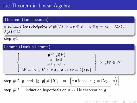
Lie Theorem in Linear Algebra

Theorem (Lie Theorem)

g solvable Lie subalgebra of gl(V ) ⇒ ∃ v ∈ V : x ∈ g xv = λ(x)v ,λ(x) ∈ C

step #1

Lemma (Dynkin Lemma)g ⊂ gl(V )a ideal∃λ ∈ a∗ :

W = {v ∈ V : ∀ a ∈ a av = λ(a)v}

⇒ gW ∈W

step # 2 g and [g, g] 6= {0}, ⇒{∃ a ideal : g = Ce0 + a

}step # 3 induction hypothesis on a Lie theorem on g

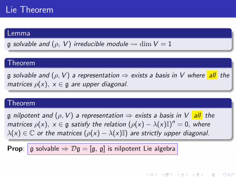
Lie Theorem

Lemma

g solvable and (ρ, V ) irreducible module dimV = 1

Theorem

g solvable and (ρ,V ) a representation ⇒ exists a basis in V where all thematrices ρ(x), x ∈ g are upper diagonal.

Theorem

g nilpotent and (ρ,V ) a representation ⇒ exists a basis in V all thematrices ρ(x), x ∈ g satisfy the relation (ρ(x)− λ(x)I)n = 0, whereλ(x) ∈ C or the matrices (ρ(x)− λ(x)I) are strictly upper diagonal.

Prop: g solvable ⇒ Dg = [g, g] is nilpotent Lie algebra

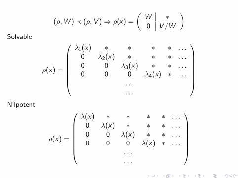
(ρ,W ) ≺ (ρ,V )⇒ ρ(x) =

(W ∗0 V /W

)Solvable

ρ(x) =

λ1(x) ∗ ∗ ∗ ∗ . . .0 λ2(x) ∗ ∗ ∗ . . .0 0 λ3(x) ∗ ∗ . . .0 0 0 λ4(x) ∗ . . .

. . .

. . .

Nilpotent

ρ(x) =

λ(x) ∗ ∗ ∗ ∗ . . .0 λ(x) ∗ ∗ ∗ . . .0 0 λ(x) ∗ ∗ . . .0 0 0 λ(x) ∗ . . .

. . .

. . .

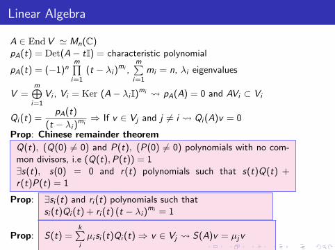
Linear Algebra

A ∈ EndV ' Mn(C)pA(t) = Det(A− tI) = characteristic polynomial

pA(t) = (−1)nm∏i=1

(t − λi )mi ,m∑i=1

mi = n, λi eigenvalues

V =m⊕i=1

Vi , Vi = Ker (A− λi I)mi pA(A) = 0 and AVi ⊂ Vi

Qi (t) =pA(t)

(t − λi )mi⇒ If v ∈ Vj and j 6= i Qi (A)v = 0

Prop: Chinese remainder theorem

Q(t), (Q(0) 6= 0) and P(t), (P(0) 6= 0) polynomials with no com-mon divisors, i.e (Q(t),P(t)) = 1∃s(t), s(0) = 0 and r(t) polynomials such that s(t)Q(t) +r(t)P(t) = 1

Prop: ∃si (t) and ri (t) polynomials such thatsi (t)Qi (t) + ri (t) (t − λi )mi = 1

Prop: S(t) =k∑iµi si (t)Qi (t)⇒ v ∈ Vj S(A)v = µjv

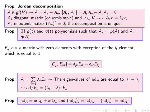
Prop: Jordan decomposition

A ∈ gl(V ) A = As + An, [As , An] = AsAn − AnAs = 0As diagonal matrix (or semisimple) and v ∈ Vi ! Asv = λiv ,An nilpotent matrix (An)n = 0, the decomposition is unique

Prop: ∃ ! p(t) and q(t) polynomials such that As = p(A) and An =q(A)

Eij n × n matrix with zero elements with exception of the ij element,which is equal to 1

[Eij , Ek`] = δjkEi` − δi`Ekj

Prop: A =n∑

i=1λiEii The eigenvalues of adA are equal to λi − λj

adAEij = (λi − λj)Eij

Prop: adA = adAs + adAn and (adA)s = adAs , (adA)n = adAn

Cartan Criteria

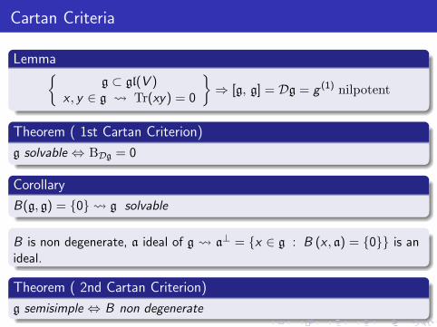
Lemma{g ⊂ gl(V )

x , y ∈ g Tr(xy) = 0

}⇒ [g, g] = Dg = g (1) nilpotent

Theorem ( 1st Cartan Criterion)

g solvable ⇔ BDg = 0

Corollary

B(g, g) = {0} g solvable

B is non degenerate, a ideal of g a⊥ = {x ∈ g : B (x , a) = {0}} is anideal.

Theorem ( 2nd Cartan Criterion)

g semisimple ⇔ B non degenerate

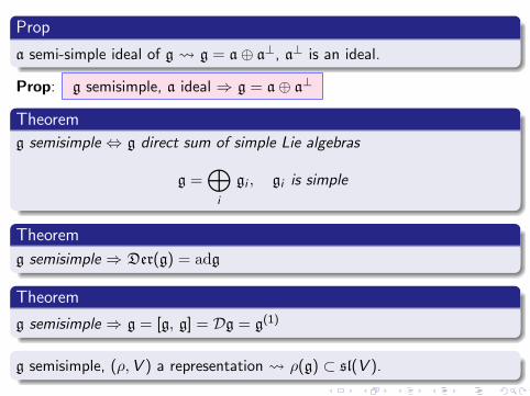
Prop

a semi-simple ideal of g g = a⊕ a⊥, a⊥ is an ideal.

Prop: g semisimple, a ideal ⇒ g = a⊕ a⊥

Theorem

g semisimple ⇔ g direct sum of simple Lie algebras

g =⊕i

gi , gi is simple

Theorem

g semisimple ⇒ Der(g) = adg

Theorem

g semisimple ⇒ g = [g, g] = Dg = g(1)

g semisimple, (ρ,V ) a representation ρ(g) ⊂ sl(V ).

Abstract Jordan decomposition

Prop: g semisimple Z (g) = {0}

Prop: g semisimple g'iso

adg

Prop: ∂ ∈ Der(g), ∂ = ∂s + ∂n the Jordan decomposition ∂s ∈ Der(g) and ∂n ∈ Der(g)

Theorem (Abstract Jordan Decomposition)

g semisimple adx = (adx)s + (adx)n Jordan decomposition andx = xs + xn where xs ∈ g, (adx)s = adxs and xn ∈ g, (adx)n = adxn

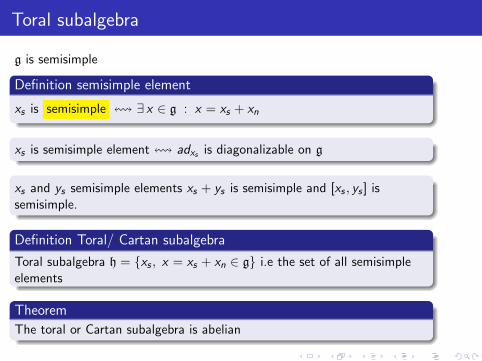
Toral subalgebra

g is semisimple

Definition semisimple element

xs is semisimple ! ∃ x ∈ g : x = xs + xn

xs is semisimple element ! adxs is diagonalizable on g

xs and ys semisimple elements xs + ys is semisimple and [xs , ys ] issemisimple.

Definition Toral/ Cartan subalgebra

Toral subalgebra h = {xs , x = xs + xn ∈ g} i.e the set of all semisimpleelements

Theorem

The toral or Cartan subalgebra is abelian

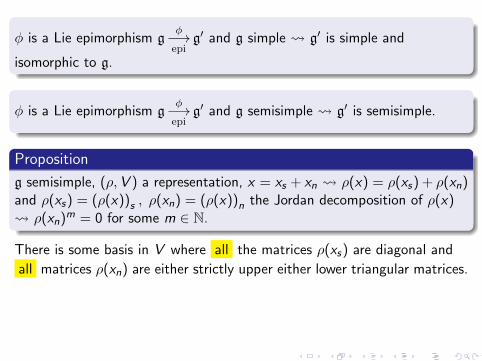
φ is a Lie epimorphism gφ−→epi

g′ and g simple g′ is simple and

isomorphic to g.

φ is a Lie epimorphism gφ−→epi

g′ and g semisimple g′ is semisimple.

Proposition

g semisimple, (ρ,V ) a representation, x = xs + xn ρ(x) = ρ(xs) + ρ(xn)and ρ(xs) = (ρ(x))s , ρ(xn) = (ρ(x))n the Jordan decomposition of ρ(x) ρ(xn)m = 0 for some m ∈ N.

There is some basis in V where all the matrices ρ(xs) are diagonal and

all matrices ρ(xn) are either strictly upper either lower triangular matrices.

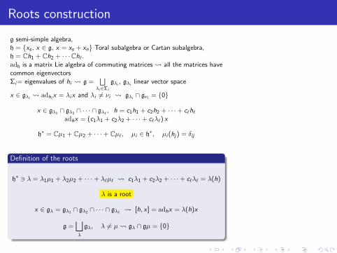
Roots construction

g semi-simple algebra,h = {xs , x ∈ g, x = xs + xn} Toral subalgebra or Cartan subalgebra,h = Ch1 + Ch2 + · · ·Ch`.adh is a matrix Lie algebra of commuting matrices all the matrices havecommon eigenvectorsΣi= eigenvalues of hi g =

⊔λi∈Σi

gλi , gλi linear vector space

x ∈ gλi adhi x = λix and λi 6= νi gλi ∩ gνi = {0}

x ∈ gλ1 ∩ gλ2 ∩ · · · ∩ gλ` , h = c1h1 + c2h2 + · · ·+ c`h`adhx = (c1λ1 + c2λ2 + · · ·+ c`λ`) x

h∗ = Cµ1 + Cµ2 + · · ·+ Cµ`, µi ∈ h∗, µi (hj) = δij

Definition of the roots

h∗ 3 λ = λ1µ1 + λ2µ2 + · · ·+ λ`µ` c1λ1 + c2λ2 + · · ·+ c`λ` = λ(h)

λ is a root

x ∈ gλ = gλ1 ∩ gλ2 ∩ · · · ∩ gλ` [h, x ] = adhx = λ(h)x

g =⊔λ

gλ, λ 6= µ gλ ∩ gµ = {0}

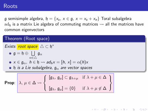
Roots

g semisimple algebra, h = {xs , x ∈ g, x = xs + xn} Toral subalgebraadh is a matrix Lie algebra of commuting matrices all the matrices havecommon eigenvectors

Theorem (Root space)

Exists root space 4 ⊂ h∗

g = h⊕⊔α∈4

gα

x ∈ gα, h ∈ h adhx = [h, x ] = α(h)xh is a Lie subalgebra, gα are vector spaces

Prop: λ, µ ∈ ∆

[gλ, gµ] ⊂ gλ+µ if λ+ µ ∈ ∆

[gλ, gµ] = {0} if λ+ µ 6∈ ∆

Semisimple roots

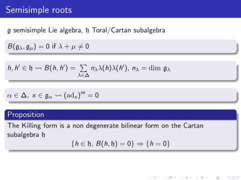
g semisimple Lie algebra, h Toral/Cartan subalgebra

B(gλ, gµ) = 0 if λ+ µ 6= 0

h, h′ ∈ h B(h, h′) =∑λ∈∆

nλλ(h)λ(h′), nλ = dim gλ

α ∈ ∆, x ∈ gα (adx)m = 0

Proposition

The Killing form is a non degenerate bilinear form on the Cartansubalgebra h

{h ∈ h, B(h, h) = 0} ⇒ {h = 0}

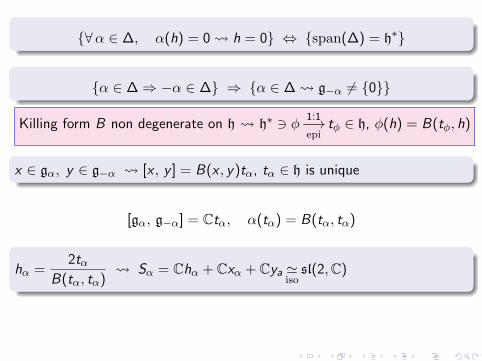
{∀α ∈ ∆, α(h) = 0 h = 0} ⇔ {span(∆) = h∗}

{α ∈ ∆⇒ −α ∈ ∆} ⇒ {α ∈ ∆ g−α 6= {0}}

Killing form B non degenerate on h h∗ 3 φ 1:1−→epi

tφ ∈ h, φ(h) = B(tφ, h)

x ∈ gα, y ∈ g−α [x , y ] = B(x , y)tα, tα ∈ h is unique

[gα, g−α] = Ctα, α(tα) = B(tα, tα)

hα =2tα

B(tα, tα) Sα = Chα + Cxα + Cya '

isosl(2,C)

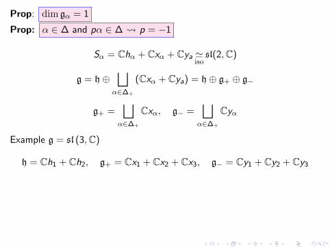
Prop: dim gα = 1

Prop: α ∈ ∆ and pα ∈ ∆ p = −1

Sα = Chα + Cxα + Cya 'iso

sl(2,C)

g = h⊕⊔

α∈∆+

(Cxα + Cya) = h⊕ g+ ⊕ g−

g+ =⊔

α∈∆+

Cxα, g− =⊔

α∈∆+

Cyα

Example g = sl (3,C)

h = Ch1 + Ch2, g+ = Cx1 + Cx2 + Cx3, g− = Cy1 + Cy2 + Cy3

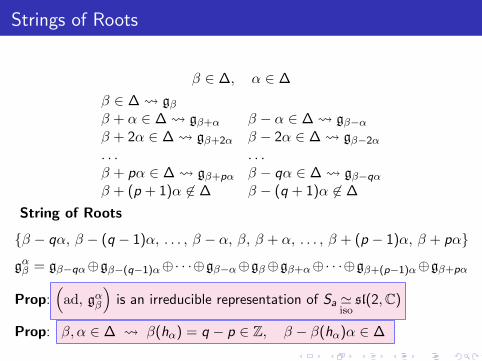
Strings of Roots

β ∈ ∆, α ∈ ∆

β ∈ ∆ gββ + α ∈ ∆ gβ+α β − α ∈ ∆ gβ−αβ + 2α ∈ ∆ gβ+2α β − 2α ∈ ∆ gβ−2α

. . . . . .β + pα ∈ ∆ gβ+pα β − qα ∈ ∆ gβ−qαβ + (p + 1)α 6∈ ∆ β − (q + 1)α 6∈ ∆

String of Roots

{β − qα, β − (q − 1)α, . . . , β − α, β, β + α, . . . , β + (p − 1)α, β + pα}

gαβ = gβ−qα⊕gβ−(q−1)α⊕· · ·⊕gβ−α⊕gβ⊕gβ+α⊕· · ·⊕gβ+(p−1)α⊕gβ+pα

Prop:(ad, gαβ

)is an irreducible representation of Sa '

isosl(2,C)

Prop: β, α ∈ ∆ β(hα) = q − p ∈ Z, β − β(hα)α ∈ ∆

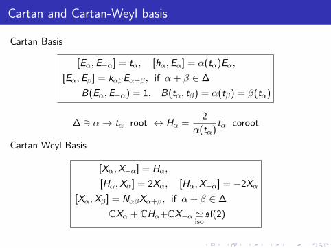
Cartan and Cartan-Weyl basis

Cartan Basis

[Eα,E−α] = tα, [hα,Eα] = α(tα)Eα,

[Eα,Eβ] = kαβEα+β, if α + β ∈ ∆

B(Eα,E−α) = 1, B(tα, tβ) = α(tβ) = β(tα)

∆ 3 α→ tα root ↔ Hα =2

α(tα)tα coroot

Cartan Weyl Basis

[Xα,X−α] = Hα,

[Hα,Xα] = 2Xα, [Hα,X−α] = −2Xα

[Xα,Xβ] = NαβXα+β, if α + β ∈ ∆

CXα + CHα+CX−α 'iso

sl(2)

Def: (α, β) ≡ B(tα, tβ) = α(tβ) = β(tα) = (β, α)

Prop: << β, α >>≡ 2 (β, α)

(α, α)= q − p ∈ Z

Prop: wα(β) ≡ β− << β, α >> α, wα(β) ∈ ∆

Def: Weyl Transform wα : ∆ −→ ∆

Prop: β − α 6∈ ∆ << β, α >>< 0,

Prop: β + α 6∈ ∆ << β, α >>> 0

Prop: β(hα) =<< β, α >>∈ Z, B(hα, hβ) =∑γ∈∆

γ(hα)γ(hβ) ∈ Z

Prop: B(hα, hα) =∑γ∈∆

(<< α, γ >>)2 > 0

Prop: β ∈ ∆ and β =m∑i=1

ciαi , αi ∈ ∆ ci ∈ Q

Prop: ∆ ⊂ spanQ(∆) = EQ, EQ is a Q-euclidean vector space.

Prop: (α, β) ≡ B(tα, tβ) ∈ Q , (α, α) > 0, (α, α) = 0 α = 0

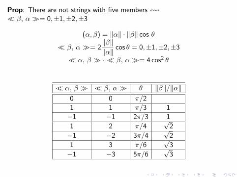
Prop: There are not strings with five members !<< β, α >>= 0,±1,±2,±3

(α, β) = ‖α‖ · ‖β‖ cos θ

<< β, α >>= 2‖β‖‖α‖

cos θ = 0,±1,±2,±3

<< α, β >> · << β, α >>= 4 cos2 θ

<< α, β >> << β, α >> θ ‖β‖/‖α‖0 0 π/2

1 1 π/3 1

−1 −1 2π/3 1

1 2 π/4√

2

−1 −2 3π/4√

2

1 3 π/6√

3

−1 −3 5π/6√

3

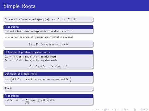
Simple Roots

∆=roots is a finite set and spanR (∆) =<< ∆ >>= E = R`

Proposition

E is not a finite union of hypersurfaces of dimension `− 1

E is not the union of hypersurfaces vertical to any root

∃ z ∈ E : ∀α ∈ ∆ (α, z) 6= 0

Definition of positive/negative roots

∆+ = {α ∈ ∆ : (α, z) > 0}, positive roots∆− = {α ∈ ∆ : (α, z) < 0}, negative roots

∆ = ∆+ ∪∆−, ∆+ ∩∆− = ∅

Definition of Simple roots

Σ ={β ∈ ∆+ : is not the sum of two elements of ∆+

}Σ 6= ∅

Proposition

β ∈ ∆+ β =∑σ∈Σ

nσσ, nσ ≥ 0, nσ ∈ Z

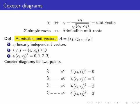
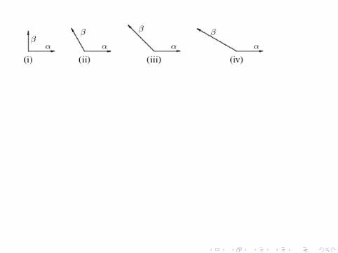
Coxeter diagrams

αi ↔ εi =αi√

(αi , αi )= unit vector

Σ simple roots ↔ Admissible unit roots

Def: Admissible unit vectors A = {ε1, ε2, . . . εn}1 εi linearly independent vectors2 i 6= j (εi , εj) ≤ 03 4 (εi , εj)

2 = 0, 1, 2, 3,

Coxeter diagrams for two points

εi◦ ◦εj 4 (εi , εj)2 = 0

εi◦ ◦εj 4 (εi , εj)2 = 1

εi◦ ◦εj 4 (εi , εj)2 = 2

εi◦ ◦εj 4 (εi , εj)2 = 3

Prop: A′ = A− {εi} admissible

Prop: The number of non zero pairs is less than n

Prop: The Coxeter graph has not cycles

Prop: The maximum number of edges is three

Prop: If {ε1, ε2, . . . , εm} ∈ A and 2 (εk , εk+1) = −1 ,|i − j | > 0 (εi , εj) = 0

ε =m∑

k=1

εk ⇒ A′ = (A− {ε1, ε2, . . . , εm})⋃{ε} admissible

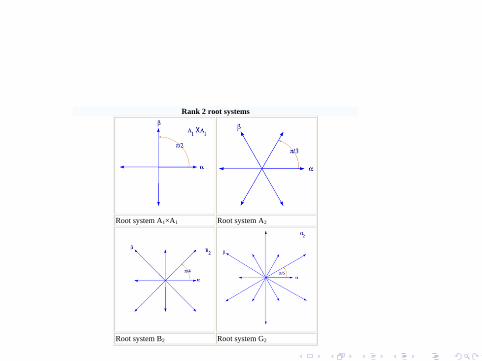
Rank 2 root systems

Root system A1×A1 Root system A2

Root system B2 Root system G2

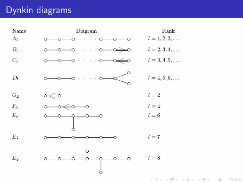
Dynkin diagrams

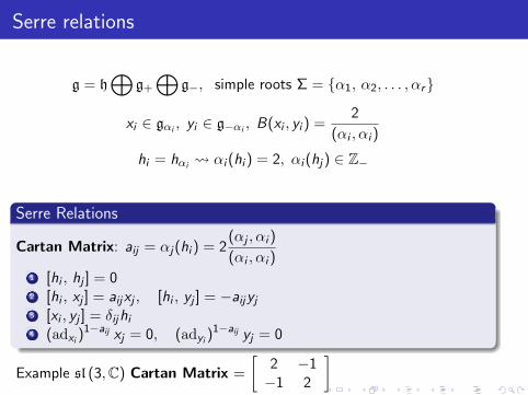
Serre relations

g = h⊕

g+

⊕g−, simple roots Σ = {α1, α2, . . . , αr}

xi ∈ gαi , yi ∈ g−αi , B(xi , yi ) =2

(αi , αi )

hi = hαi αi (hi ) = 2, αi (hj) ∈ Z−

Serre Relations

Cartan Matrix: aij = αj(hi ) = 2(αj , αi )

(αi , αi )1 [hi , hj ] = 02 [hi , xj ] = aijxj , [hi , yj ] = −aijyj3 [xi , yj ] = δijhi4 (adxi )

1−aij xj = 0, (adyi )1−aij yj = 0

Example sl (3,C) Cartan Matrix =

[2 −1−1 2

]

Weight ordering

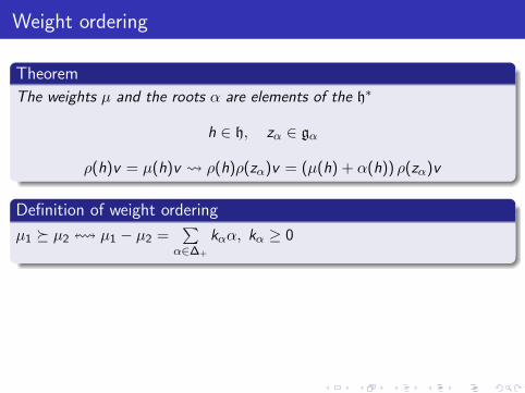
Theorem

The weights µ and the roots α are elements of the h∗

h ∈ h, zα ∈ gα

ρ(h)v = µ(h)v ρ(h)ρ(zα)v = (µ(h) + α(h)) ρ(zα)v

Definition of weight ordering

µ1 � µ2 ! µ1 − µ2 =∑

α∈∆+

kαα, kα ≥ 0

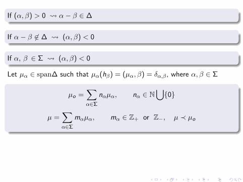
If (α, β) > 0 α− β ∈ ∆

If α− β 6∈ ∆ (α, β) < 0

If α, β ∈ Σ (α, β) < 0

Let µα ∈ span∆ such that µα(hβ) = (µα, β) = δα,β, where α, β ∈ Σ

µo =∑α∈Σ

nαµα, nα ∈ N⋃{0}

µ =∑α∈Σ

mαµα, mα ∈ Z+ or Z−, µ ≺ µo

Highest weight

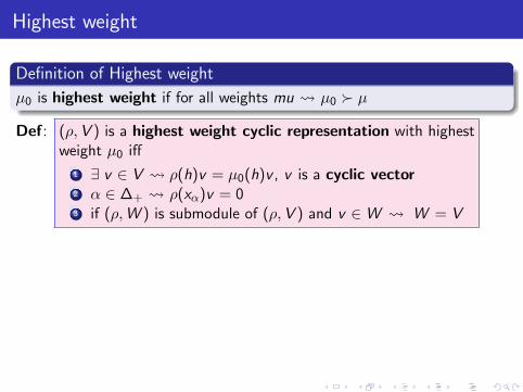
Definition of Highest weight

µ0 is highest weight if for all weights mu µ0 � µ

Def: (ρ,V ) is a highest weight cyclic representation with highestweight µ0 iff

1 ∃ v ∈ V ρ(h)v = µ0(h)v , v is a cyclic vector2 α ∈ ∆+ ρ(xα)v = 03 if (ρ,W ) is submodule of (ρ,V ) and v ∈W W = V

Highest weight representation

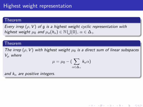
Theorem

Every irrep (ρ,V ) of g is a highest weight cyclic representation withhighest weight µ0 and µo(hα) ∈ N

⋃{0}, α ∈ ∆+

Theorem

The irrep (ρ,V ) with highest weight µ0 is a direct sum of linear subspacesVµ where

µ = µ0 − (∑α∈∆+

kαα)

and kα are positive integers.

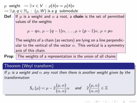
µ weight ∃ v ∈ V : ρ(h)v = µ(h)v ∃ p, q ∈ No : (ρ,W ) is a g submodule

Def: If µ is a weight and α a root, a chain is the set of permittedvalues of the weights

µ− qα, µ− (q − 1)α, . . . , µ+ (p − 1)α, µ+ pα

The weights of a chain (as vectors) are lying on a line perpendic-ular to the vertical of the vector α. This vertical is a symmetryaxis of this chain.

Prop: The weights of a representation is the union of all chains

Theorem (Weyl transform)

If µ is a weight and α any root then there is another weight given by thetransformation

Sα (µ) = µ− 2(µ, α)

(α, α)α and 2

(µ, α)

(α, α)∈ Z