Kansas Geological Survey

User’s Guide to HyDRA_Translate.xlsm: An Excel Workbook for Quantification of Water Well Drillers’ Logs

Geoffrey C. Bohling Kansas Geological Survey

University of Kansas

Kansas Geological Survey Open-File Report No. 2016-30 December 2016

The University of Kansas, Lawrence, KS 66047 (785) 864-3965 www.kgs.ku.edu

KANSAS GEOLOGICAL SURVEY OPEN-FILE REPORT

>>>>>>>>>> NOT FOR RESALE <<<<<<<<<<

Disclaimer

The Kansas Geological Survey made a conscientious effort to ensure the accuracy of this report. However, the Kansas Geological Survey does not guarantee this document to be completely free from errors or inaccuracies and disclaims any responsibility or liability for interpretations based on data used in the production of this document or decisions based thereon. This report is intended to make results of research available at the earliest possible date but is not intended to constitute formal publication.

1

Introduction This report explains how to use the macro-enabled Excel workbook HyDRA_Translate.xlsm. The workbook implements a few of the steps in the HyDRA (Hydrostratigraphic Drilling Record Assessment) processing sequence. The overall objective of the HyDRA process, which is an extension of the earlier PST+ project (Macfarlane and Schneider, 2007; Macfarlane, 2009), is to develop three-dimensional (3D) aquifer property models from water well drillers’ logs. The basic approach is to convert the verbatim sediment (or lithology) descriptions in the logs into a 3D point dataset representing volumetric proportions of material in a reasonably small set of sediment classes or categories and then interpolate those proportions to a 3D grid (e.g., a flow model grid). Aquifer properties in each grid cell can then be computed based on the category proportions in that grid cell. A program implementing the full set of processing steps is under development but is not yet available. This workbook provides users an immediate means to perform the steps that are unique to the processing of drillers’ logs. Specifically, HyDRA_Translate.xlsm implements the three steps involved in getting from a set of verbatim logs to a 3D point dataset that represents the category proportions in a sequence of regularly spaced intervals in the logged wells. These steps are referred to as standardization, categorization, and segmentation. Standardization is the process of mapping the verbatim sediment description for each logged depth interval into one or more standardized lithology codes, along with a set of percentages associated with the standardized lithologies. (The term “sediment type” would be more accurate than “lithology” in many cases, but this documentation will continue to use “lithology.”) For example, “lime green sand with streaks of fuchsia clay and a bit of baby blue gravel” might be represented as 70% snd (sand), 20% c (clay), and 10% g (gravel). This translation process uses a translation table that maps each unique sediment description into a standardized representation. Building the translation table is a labor-intensive and subjective process, since a standardized representation of each description has to be entered by hand. The degree of subjectivity involved in assigning each standardized representation varies with the degree of ambiguity of the description, which can range from quite clear to highly ambiguous. Categorization is the process of converting the standardized lithology proportions in each logged interval into proportions of material in a smaller number of sediment categories, based on a table specifying the category into which each standardized lithology falls. KGS modeling projects have used a set of 71 standardized lithologies and mapped them into five to eight categories, with the number of categories and category assignments varying to meet the needs of each project. The workbook contains an example lithology/category worksheet listing these 71 lithology codes and two example categorizations, one using five categories and another using eight categories. The rationale behind the separation of standardization and categorization into separate steps is that the standardized representations of a set of verbatim descriptions should be

2

useful for a number of different purposes, while the categorization of the standardized lithologies might change fairly often, to meet the needs of different projects or for modeling different properties within the same project (e.g., different categorizations for hydraulic conductivity and specific storage). Segmentation is the process of dividing each well into a sequence of regular intervals (e.g., 10-foot intervals) and computing the category proportions within each of those regular intervals based on the category proportions in all the logged intervals that fall within or overlap each regular interval. The segmentation is based on elevation, rather than depth, and the process also adds geographic (X and Y) coordinates. The end result is a 3D point dataset of category proportions (with the Z coordinate of each point being the center elevation of the regular interval). To run this process, you need to provide coordinate information for the wells, including surface elevation and X and Y coordinates. However, you may provide all zeros for the coordinate values if no coordinate information is available. Supplying zeros for the surface elevation values leads to segmenting the wells based on negative depth. HyDRA_Translate.xlsm does not include code for importing logs or extracting them from a database—you have to provide a worksheet with the logs—nor does it include code for the subsequent steps of interpolating the category proportions to a 3D grid or computing property values based on the proportions. Those steps will be included in the complete HyDRA processing system. Other important operations not included in the workbook are exploratory analysis and visualization of the logs. However, the workbook includes routines that assist with error identification and quality control and with management of the translation table.

Workbook Overview The controls for the three steps are contained in spreadsheets named Standardize, Categorize, and Segment, referred to hereafter as the control worksheets. The Visual Basic code implementing each step is attached to the corresponding worksheet. The Standardize worksheet also contains controls and code for three data-checking processes that you might want to run before you standardize the logs. Each process asks for the names of two or three input worksheets that must be included in the workbook containing the code. These are specified by entering the worksheet name in the appropriate cell in the control worksheet (always in column F, in the row indicated by a text “prompt”). One way to enter a data worksheet name into the appropriate cell is to double-click on the data worksheet’s tab to highlight the name, use Ctrl-C to copy that name, and Ctrl-V to paste it into the cell. Each process attempts to produce a set of output worksheets with fixed names (for example, StandardizedLogs). An error will occur if a worksheet with one of those names already exists in the workbook when you run the process. Consequently, before you re-run a process, you need

3

to rename or delete any existing output worksheets from that process or move them to another workbook. Since the example workbook contains a complete set of output worksheets, you will need to delete, move, or rename those before you can generate your own. A convention for the various data worksheets, both input and output, is that labels occur in row 5, with data starting in row 6. When processing input data, the code will read down from row 6 until it encounters an empty cell in column A, at which point it will stop processing. Therefore, you should make sure that there are no empty cells in column A in the range of data that you want to process. You can make multiple copies of the workbook and the Visual Basic code will be included in any new copies of the control worksheets. However, this is not be an ideal approach if you are considering the possibility of modifying the Visual Basic code (which is open for modification), since you would then have multiple workbooks containing copies of the code and would have to modify each one to maintain consistency. Another approach would be to use only one copy of the workbook containing the control worksheets and move data worksheets into and out of that workbook. Input Worksheet Layouts Four input data worksheets are used by the processing steps. These worksheets contain 1) the logs to be processed, 2) the translation table, 3) the list of standardized lithology codes and category assignments, and 4) the well coordinates. You may name these worksheets anything you want. The layouts for these worksheets are described below. Log data worksheet The worksheet containing the logs to be processed should be laid out as shown in fig. 1.

Figure 1. Example input log worksheet (ShermanCoLogs21Sept2016).

4

These example data are all the logs from Sherman County, Kansas, that had been transcribed into the Kansas Geological Survey’s WWC5 database, specifically into the WWC5_LOGS table, as of September 13, 2016. The logs are from 861 wells, with a total of 11,638 depth intervals. No quality control has been applied to these logs; in fact, there are problems with the interval depths in several of the wells. Nothing above row 6 or to the right of column E in the log worksheet matters to the Visual Basic code. The code just expects to find the data starting in row 6, with the county name in column A, well ID in column B, interval top depth in column C, bottom depth in column D, and verbatim sediment description in column E. You may label these columns anything you want. The code does nothing with the county name except pass it along, so column A could actually contain anything; however, the first blank cell in column A below row 5 is taken to signal the end of the data. The well (or borehole) IDs in this example data are the well sequence numbers from the WWC5 database. You can use anything for the IDs, as long as the ID for each well is unique. The code handles the IDs as character strings, not numbers. The TopDepth and BotDepth columns in the example log worksheet correspond to the fields labeled FROM_ELEV and TO_ELEV in WWC5_LOGS. Although the data shown in Figure 1 are ordered by Well ID and then TopDepth (increasing), none of the Visual Basic code depends on the data order except for the code that checks for problems in the depth data (the code behind the Check Interval Depths button on the Standardize worksheet), which assumes that the data values are grouped (but not necessarily ordered) by Well ID and sorted by increasing interval depth within each well. Translation Table A translation table worksheet should be laid out as shown in fig. 2.

Figure 2. Example translation table worksheet (TranslationTable26Oct2016).

5

Nothing above row 6 or to the right of column C in the translation table worksheet matters to the Visual Basic code. The code expects to find a list of verbatim sediment descriptions in column A, starting in row 6. For each description, column B contains a comma-delimited list of percentages and column C a corresponding comma-delimited list of standardized lithology codes (all of which should appear in the list of “authorized” codes contained in the lithology code worksheet). As an example, row 8 in fig. 2 says that the verbatim description “sand and sand rock strips” should be translated as 80% sand (snd) and 20% cemented sand or gravel (cesd/cg). In the translation process, descriptions are converted to all lower case and stripped of leading and trailing white space. Otherwise, any difference between two descriptions (for example, “lime hard” versus “lime, hard”) results in those two descriptions being considered distinct. Lithology Code Worksheet The example lithology code worksheet included in the workbook is shown in fig. 3.

Figure 3. Example lithology code worksheet (LithologyCodes). The list of standardized lithology codes appears in column A, starting in row 6. These are used in the process of checking the entries in the translation table. The descriptions in column B are simply documentation; the code does nothing with them. Columns C and D in this sheet contain example assignments of the codes to sediment type categories, one grouping the standardized lithologies into eight categories and another grouping them into five categories. The category memberships are represented as integers ranging from 1 to the number of categories (8 or 5 in the example). (More accurately, the code takes the number of categories to be the largest

6

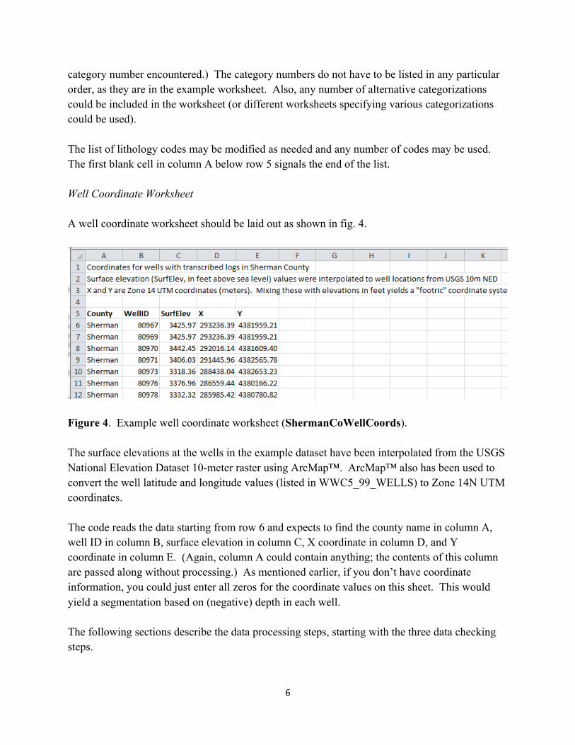
category number encountered.) The category numbers do not have to be listed in any particular order, as they are in the example worksheet. Also, any number of alternative categorizations could be included in the worksheet (or different worksheets specifying various categorizations could be used). The list of lithology codes may be modified as needed and any number of codes may be used. The first blank cell in column A below row 5 signals the end of the list. Well Coordinate Worksheet A well coordinate worksheet should be laid out as shown in fig. 4.

Figure 4. Example well coordinate worksheet (ShermanCoWellCoords). The surface elevations at the wells in the example dataset have been interpolated from the USGS National Elevation Dataset 10-meter raster using ArcMap™. ArcMap™ also has been used to convert the well latitude and longitude values (listed in WWC5_99_WELLS) to Zone 14N UTM coordinates. The code reads the data starting from row 6 and expects to find the county name in column A, well ID in column B, surface elevation in column C, X coordinate in column D, and Y coordinate in column E. (Again, column A could contain anything; the contents of this column are passed along without processing.) As mentioned earlier, if you don’t have coordinate information, you could just enter all zeros for the coordinate values on this sheet. This would yield a segmentation based on (negative) depth in each well. The following sections describe the data processing steps, starting with the three data checking steps.

7

Check Interval Depths The buttons for launching the three data-checking procedures are included on the Standardize worksheet (fig. 5).

Figure 5. The Standardize worksheet, including buttons for launching the three data-checking procedures. Clicking on the Check Interval Depths button will launch code that checks for problems in the interval depths in the input log worksheet whose name is given in cell F4 (ShermanCoLogs21Sept2016 in the example). The code will flag the following problems: 1) missing interval depths, either top or bottom, 2) negative interval thicknesses (interval bottom depth less than interval top depth), and 3) inconsistencies in the sequence of interval depths (e.g., an interval top depth less than the preceding interval bottom depth). In performing the third check, the code assumes that the logs are grouped by well ID and sorted by increasing interval depth within each well—or in a way that is intended to yield increasing interval depths, for example, by increasing top depth. If the logs are not sorted in this fashion, then the depth check will produce an overwhelming number of error messages. The depth-checking code is the only code in the workbook that depends on the ordering of the log data. The depth values do not have any impact on the standardization and categorization steps; these steps simply pass along the depths, without processing, to their output worksheets. The depths come into play during the segmentation process, but that code does not depend on the sorting of the data. However, errors in the depths will have some impact on the segmentation results. For that reason—and to provide some basic quality control—it is reasonable to sort the logs by well ID and depth to allow checking for such errors using the depth-checking code. This can easily be accomplished using Excel’s data sorting options (on the Data tab), sorting first by well ID and then by interval top depth (increasing).

8

The interval depth checking code will produce an output worksheet named IntervalDepthCheck. Figure 6 shows the upper portion of the IntervalDepthCheck worksheet for the Sherman County log data.

Figure 6: Upper portion of output worksheet (IntervalDepthCheck) produced by running depth-checking code on Sherman County log data. Missing bottom depths are fairly common, since drillers will often list only a top depth for the last interval in a well, when they have reached bedrock. The segmentation process will ignore logged intervals with missing depths (bottom or top) and will also ignore intervals with negative thicknesses. Several wells in this dataset exhibit inconsistencies in the interval depths (e.g., an interval top depth that is less than the previous interval’s bottom depth) leading to apparently overlapping logged intervals. In the segmentation process, this results in too much material being assigned to one or more of the regular intervals in a well. The segmentation process does not write output results for such intervals. The logical next step after running the depth-checking code would be to edit the data to address the identified problems. However, this documentation will continue to use the unedited data.

9

Interval Statistics Clicking on the Interval Statistics button in the Standardize worksheet (fig. 5) will launch code that computes the average thickness of the logged intervals in each well plus some related measures intended to help with quality control. For example, one might consider removing from the dataset wells that have only a few very thick intervals, as indicated by abnormally high average interval thicknesses. It is also advisable to check for wells with anomalously large maximum depths. The code will produce an output worksheet named IntervalStats. Figure 7 shows the IntervalStats worksheet for the Sherman County logs.

Figure 7. IntervalStats worksheet produced using the Sherman County logs. The columns are Well ID, Minimum Depth, Maximum Depth, Number of Intervals, Total Thickness, Average Interval Thickness, Number of Surface Intervals, Surface Interval Thickness, and Average Interval Thickness Excluding Surface Interval. The first six column labels (Well ID through Average Interval Thickness) are self-explanatory. The total thickness will be the same as the difference between the maximum and minimum depths except when there are problems in the depth values (e.g., negative thickness intervals, which do not contribute to the total thickness). A surface interval is an interval with a top depth of zero. In general, the number of surface intervals (column G) will either be 1, when the log starts from ground surface, or 0, when it starts somewhere below ground surface. A number greater than 1 in this column indicates that the well contains more than one interval starting from ground surface. The surface interval thickness is listed in column H to aid in the identification of logs with extremely thick surface intervals, which are fairly common. Because a very thick surface interval might lead to a large overall average interval thickness in a log that is otherwise

10

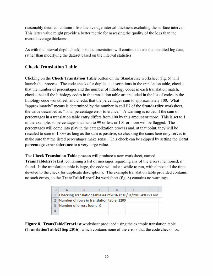
reasonably detailed, column I lists the average interval thickness excluding the surface interval. This latter value might provide a better metric for assessing the quality of the logs than the overall average thickness. As with the interval depth check, this documentation will continue to use the unedited log data, rather than modifying the dataset based on the interval statistics. Check Translation Table Clicking on the Check Translation Table button on the Standardize worksheet (fig. 5) will launch that process. The code checks for duplicate descriptions in the translation table, checks that the number of percentages and the number of lithology codes in each translation match, checks that all the lithology codes in the translation table are included in the list of codes in the lithology code worksheet, and checks that the percentages sum to approximately 100. What “approximately” means is determined by the number in cell F7 of the Standardize worksheet, the value described as “Total percentage error tolerance.” A warning is issued if the sum of percentages in a translation table entry differs from 100 by this amount or more. This is set to 1 in the example, so percentages that sum to 99 or less or 101 or more will be flagged. The percentages will come into play in the categorization process and, at that point, they will be rescaled to sum to 100% as long as the sum is positive, so checking the sums here only serves to make sure that the listed percentages make sense. This check can be skipped by setting the Total percentage error tolerance to a very large value. The Check Translation Table process will produce a new worksheet, named TransTableErrorList, containing a list of messages regarding any of the errors mentioned, if found. If the translation table is large, the code will take a while to run, with almost all the time devoted to the check for duplicate descriptions. The example translation table provided contains no such errors, so the TransTableErrorList worksheet (fig. 8) contains no warnings.

Figure 8. TransTableErrorList worksheet produced using the example translation table (TranslationTable21Sept2016), which contains none of the errors that the code checks for.

11

Standardization

For convenience, the screenshot of the standardization control worksheet is repeated in fig. 9.

Figure 9. The standardization control worksheet (Standardize). The two input worksheets used in the standardization process are the worksheet containing the logs, here ShermanCoLogs21Sept2016, and the worksheet containing the translation table, here TranslationTable21Sept2016. The standardization process searches the translation table for a description matching the one in a given depth interval in the logs (after converting to lowercase and stripping leading and trailing whitespace). If a match is found, the process writes out the information for that depth interval and appends the lists of percentages and standardized lithology codes (referred to as the standardized representation). If a match is not found in the translation table, then the information for the interval is written out without a standardized representation appended. This step alone could easily be accomplished using one of Excel’s LOOKUP functions. However, the standardization code in HyDRA_Translate.xlsm does considerably more than this, primarily to help with the management of the translation table. The standardization process produces five output worksheets. The first of these, named StandardizationSummary, contains a summary of the standardization process (fig. 10). The messages in the summary worksheet are fairly self-explanatory. The depth intervals not translated are those for which no matching description was found in the translation table. The unmatched descriptions are the descriptions that still need to be translated to yield a complete translation of all the logs. In this case, there are 1,399 descriptions that need to be translated.

12

Figure 10. StandardizationSummary worksheet produced using the example log data and translation table. The second output worksheet, named StandardizedLogs, contains the logs with the addition of the matching standardized representations (fig. 11). Although none are shown in fig. 11, untranslated depth intervals are also included in the output, with empty cells in columns F and G.

Figure 11. StandardizedLogs worksheet produced using the example logs and translation table.

13

The third output worksheet, named MatchedDescriptions, contains a list of all the descriptions from the translation table that were matched (and thus used) in translating the input logs (fig. 12).

Figure 12: MatchedDescriptions worksheet produced using the example logs and translation table. As indicated in the StandardizationSummary worksheet (fig. 10), all 1,200 of the 1,200 translation table entries are matched in this example, so they are all written to the MatchedDescriptions worksheet. This has occurred because the example translation table was built for this particular dataset; in general, the translation table could contain a number of entries that are not employed in the process of translating a particular set of logs and thus only a subset of the translation table entries would be written to the MatchedDescriptions worksheet. This listing can be thought of as the project-specific translation table. Assuming that the project is focused on a reasonably small area relative to that represented in the full translation table, the MatchedDescriptions worksheet will contain far fewer entries than the full translation table. In such a case, it would be easier to work with the more limited listing, checking it for consistency and relevance to the particular project, than to work with the full translation table. Column D contains the number of occurrences of each of these descriptions in the input logs. For example, 212 depth intervals listed in ShermanCoLogs21Sept2016 are described as “top soil.” Sorting the entries in decreasing order by number of occurrences can help to prioritize the entries for quality control purposes.

14

The fourth output worksheet, named UnmatchedDescriptions, is the listing of all the descriptions in the input logs for which no matching description was found in the translation table (fig. 13).

Figure 13. UnmatchedDescriptions worksheet produced using the example logs and translation table. As indicated by the StandardizationSummary worksheet (fig. 10), there are 1,399 unmatched descriptions in this case. These are the descriptions that need to be translated and added to the translation table to obtain a complete standardization of the input logs. Columns B and C are empty; they simply serve as placeholders for the lists of percentages and lithology codes that need to be added. Column D lists the number of occurrences of each description (number of depth intervals in which it appears). Sorting the entries by number of occurrences (largest to smallest) helps to identify the amount of “mileage” you’ll get out of each translation (fig. 14).

Figure 14. Unmatched descriptions sorted by number of occurrences.

15

The final output worksheet produced by the standardization process, named WellIntervalCounts, is a listing of the number of untranslated depth intervals in each well (fig. 15).

Figure 15. WellIntervalCounts worksheet produced using example logs and translation table. One way to use this information is to sort the list in increasing order by the number of untranslated intervals to identify those wells that need only one or a few descriptions translated to be complete, find those intervals in the standardized logs, and translate the associated descriptions. (The wells with zero untranslated intervals are, of course, already complete.) You can combine this with location information to identify the wells that will be most effective for filling gaps between the existing completed wells—e.g., post all the complete wells on a map along with those that have only a few untranslated intervals and identify the wells in the latter group that do the best “gap filling.” Categorization Categorization is the process of mapping the standardized lithology percentages in each logged interval into category proportions, based on the categories into which the standardized lithologies fall. Consider a case in which the standardized representation consists of three lithologies with percentages of 50%, 30%, and 20%. If all three lithologies fall in category 3, then the interval is 100% category 3. If the first and third lithologies are in category 4 and the second is in category 2, then the interval is 70% category 4 and 30% category 2. And so forth.

16

The control sheet for the categorization process, named Categorize, is shown in fig. 16.

Figure 16: Categorization control worksheet, named Categorize. The input data are a set of standardized logs, as produced in the previous step, and a set of category assignments for the standardized lithologies. In this example, the category assignments are taken from column D of LithologyCodes, the same worksheet used to check the entries in the translation table earlier (fig. 3). Column D breaks down the 71 lithologies into five categories. You are free to modify the input worksheet names in cells F4 and F5 to suit your purposes. For example, you may be working with several different sets of standardized logs in different worksheets. The categorization process produces two output worksheets. The first, named CategorizationSummary, contains a set of messages summarizing the categorization run (fig. 17).

Figure 17. CategorizationSummary worksheet produced using example data.

17

The categorization process writes output only for depth intervals that have standardized representations—those that were matched and translated during the standardization process. It skips depth intervals with empty cells in columns F or G in the standardized log worksheet. It also skips depth intervals with certain problems and writes a warning message regarding the problem to the summary sheet (none in this example). The problems that get flagged are a mismatch in number between percentages and standardized lithology codes, unrecognized lithology codes, and percentages that sum to zero or less. The second output worksheet, named CategorizedLogs, contains the categorized version of the logs (fig. 18).

Figure 18: CategorizedLogs worksheet produced using example data. The next step, segmentation, reads the number of categories from cell F4 of this worksheet, so this cell should not be altered. The fundamental output of the categorization process is the set of category proportions starting in column I (CatProp01 through CatProp05 in this example). These are now cast in decimal form (summing to 1), rather than percentage form. The values in columns E–H provide summary information regarding the category proportions. Pmax (column G) is the maximum category proportion value. DomCat (column E) is the dominant category, meaning the category whose proportion is Pmax. It is not too uncommon to have multiple categories with proportions equal to Pmax (for, example a 50-50 split between two categories). In the case of a tie, the value of DomCat is selected at random from the set of categories whose proportions equal Pmax. Because they are selected at random, these DomCat values could change between different runs using the same data. AveCat (column F) is the proportion-weighted average category number, given by

18

𝐴𝑣𝑒𝐶𝑎𝑡 = 𝑝!𝑘!

!!!

where 𝑘 is the category number, 𝑝! is the category proportion, and 𝑁 is the number of categories. Before you use AveCat, you should consider whether it actually means anything in the problem you are working on. If the category numbers are simply names or labels for the categories, with no order implied, then AveCat means nothing. If the numbers do represent an ordering of the lithologies (e.g., in terms of increasing permeability), then AveCat does provide a general representation of trends in the data, but only in a fairly qualitative sense. AveCat should not be taken too literally because the category numbers do not represent a quantitative metric. For example, there could be a much greater difference in property values between categories 3 and 2 than between categories 2 and 1. In addition, a given average category number could represent many very different combinations of sediment categories. For example, there are an infinite number of ways of getting AveCat = 3 in an interval, including 100% category 3, a 50-50 split between categories 2 and 4, a 50-50 split between categories 1 and 5, etc., and these different combinations could have very different implications for the properties of that interval. Given a set of property (e.g., hydraulic conductivity or specific storage) values for the categories, you could compute proportion-weighted average property values for the intervals based on the category proportions and a set of category-specific property values. This will be discussed further below. Entropy (column H) is a measure of the degree of mixing of the categories in each interval. Entropy ranges from 0 for intervals with only one category (minimal mixing) to 1 for intervals with equal proportions of all the groups (maximal mixing). The formula for entropy is

𝐸𝑛𝑡𝑟𝑜𝑝𝑦 = −1ln𝑁 𝑝!ln 𝑝!

!

!!!

where 𝑝!ln 𝑝! is taken to be zero when 𝑝! = 0.

19

Segmentation Segmentation is the process of slicing each well into a sequence of regular-thickness intervals and computing the category proportions in each of those regular intervals based on the category proportions in the overlapping logged intervals (fig. 19).

Figure 19: Illustration of the process of computing category proportions in a regular interval (right) based on category proportions in the logged intervals (left) that fall within or overlap the regular interval.

20

The segmentation control sheet, named Segment, is shown in fig. 20.

Figure 20: Segmentation control worksheet (Segment). The input data are a set of categorized logs, generated in the previous step, and the well coordinate values. You specify the desired regular interval thickness in cell F9. The top and bottom elevation of each regular interval will be an even multiple of the specified thickness, and the Z (elevation) coordinate written to the output sheet for that interval will be the center of the interval. For example, if you ask for 10-foot thick intervals, the interval boundary elevations will be at even 10’s and the Z coordinate values will be at the intermediate 5’s. Regular intervals at the tops and bottoms of wells will generally not be completely overlapped (or filled) by logged intervals, leading to a total footage of material less than the specified regular interval thickness in these particular intervals. The minimum allowed footage, specified in cell F10, is the minimum amount of material that a regular interval must contain in order for the values for that interval to be written to the output sheet. In this example, regular intervals containing less than 1 foot of material will not be written to the output worksheet. Intervals can also come up short on material when there are problems with the depths listed in the logs, such as missing depths or negative interval thicknesses. An opposite problem can happen if problems with the logged depths lead to apparently overlapping logged intervals, in which case a regular interval can end up being assigned a total footage of material that is greater than the regular interval thickness. When this happens, an error message is generated saying that the interval contains “too much stuff” and the results for that interval are not written to the output sheet. The segmentation process produces two output sheets. The first, named SegmentationSummary, contains a summary of the segmentation run and a list of any warnings generated during the process (fig. 21).

21

Figure 21. SegmentationSummary worksheet generated using the example data. Because interval depth errors in several of the Sherman County wells lead to apparently overlapping logged intervals, 185 regular intervals end up with “too much stuff” and are not written to the output worksheet of segmented logs. The second output worksheet, named SegmentedLogs, contains the segmented logs (fig. 22).

Figure 22. SegmentedLogs worksheet produced using the example data. The X and Y coordinates listed here are simply transferred from the well coordinates worksheet. As mentioned above, the Z coordinate listed is the elevation of the center of the regular interval.

22

The value Level is the Z index of the regular interval, numbered upward from the lowest interval in the dataset. (The bottom of regular interval, or level, number 1 is the lowest elevation encountered in the log data rounded down to the nearest 10 feet, or whatever regular interval thickness you might use.) SedThk (sediment thickness, column G) represents the actual footage of material contained in the regular interval. Most of these values will be equal to the interval thickness, but, as mentioned above, will generally be less than that value at the tops and bottoms of wells and might be less than that value due to depth problems in the logs. The remaining columns have the same interpretation as for the categorized logs, except that they now apply to the regular intervals rather than the logged intervals. Property Calculations The next steps in the HyDRA processing sequence are to interpolate the category proportion values in the SegmentedLogs worksheet to the cells of a regular grid and then compute proportion-weighted average property values in each grid cell based on the category proportions in that cell and a set of category-specific property values. However, it is impractical to implement these steps in an Excel workbook. You can, of course, compute proportion-weighted average property values for either the logged intervals in the worksheet of categorized logs or for the regular intervals in the worksheet of segmented logs. For example, a proportion-weighted arithmetically averaged hydraulic conductivity value for each interval could be computed as

𝐾!"#$! = 𝑝!𝐾!

!

!!!

where 𝑖 is the category index and 𝐾! is the hydraulic conductivity for category 𝑖. Other kinds of averages, such as a proportion-weighted harmonic average

𝐾!!"# = 𝑝!𝐾!!!!

!!!

!!

,

can also be computed, as appropriate. These interval-averaged property values can then be interpolated to a 3D grid as well. However, an advantage of interpolating the proportions and then computing the properties in the grid cells based on the interpolated proportions is that this process will have some chance of representing sharp interfaces in the property structure—for example, you could have category 5 occurring

23

adjacent to category 2—whereas computing the properties in the wells and then interpolating them will necessarily result in smooth variation in the properties. In addition, interpolating the proportions allows for a more efficient model calibration process, since the interpolation step only needs to happen once, in advance of the calibration. Calibration then involves adjusting the category-specific property values and multiplying them by the proportion grids, which remain fixed. In contrast, computing the properties at the wells and then interpolating them to the model grid would require executing the interpolation step during every iteration of the calibration process. Figure 23 shows an example of computing proportion-weighted arithmetically averaged K values for the regular intervals in the SegmentedLogs worksheet, calling Excel’s SUMPRODUCT function to compute the sum of the products of a set of example category-specific K values and the category proportions in each interval.

Figure 23. Example computation of proportion-weighted average K values in regular intervals in the SegmentedLogs worksheet. The formula box at the top contains the formula for computing the value in cell R6.

24

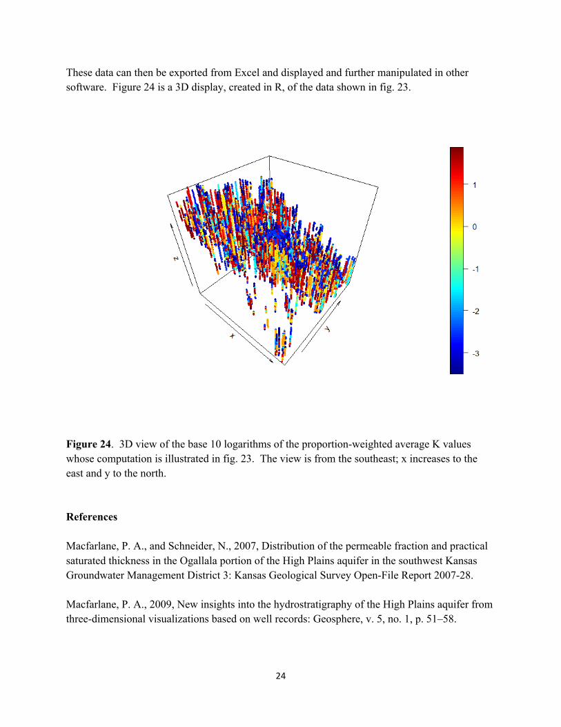
These data can then be exported from Excel and displayed and further manipulated in other software. Figure 24 is a 3D display, created in R, of the data shown in fig. 23.

Figure 24. 3D view of the base 10 logarithms of the proportion-weighted average K values whose computation is illustrated in fig. 23. The view is from the southeast; x increases to the east and y to the north. References Macfarlane, P. A., and Schneider, N., 2007, Distribution of the permeable fraction and practical saturated thickness in the Ogallala portion of the High Plains aquifer in the southwest Kansas Groundwater Management District 3: Kansas Geological Survey Open-File Report 2007-28. Macfarlane, P. A., 2009, New insights into the hydrostratigraphy of the High Plains aquifer from three-dimensional visualizations based on well records: Geosphere, v. 5, no. 1, p. 51–58.