User’s Guide for interflex

A STATA Package for Producing Flexible Marginal Effect Estimates

Yiqing Xu (Maintainer) Jens Hainmueller Jonathan Mummolo Licheng Liu

Description: interflex performs diagnostics and generates visualizations of multiplicative in-

teraction models. Besides conventional linear interaction models, it provides two additional esti-

mation strategies—linear regression based on pre-specified bins and locally linear regressions based

on Gaussian kernel reweighting—to flexibly estimate the conditional marginal effect of a treatment

variable on an outcome variable across different values of a moderating variable. These approaches

relax the linear interaction effect assumption and safeguard against excessive extrapolation.

Citation: Jens Hainmueller, Jonathan Mummolo, and Yiqing Xu. 2016. “How Much Should

We Trust Estimates from Multiplicative Interaction Models? Simple Tools to Improve Empirical

Practice.” Available at SSRN: https://papers.ssrn.com/abstract_id=2739221.

This version: 1.0.1 (Comments and suggestions greatly appreciated!)

Date: March 5, 2017

Contents

(1) Installation

(2) Examples 1 and 2: Linear marginal effects

(3) Example 3: Nonlinear marginal effects

(4) Example 4: Nonlinear marginal effects with fixed effects

1

Installation

Install from SSC. You can install the package from the Boston College Statistical Software

Components (SSC) archive. Simply type the following command in STATA:

. ssc install interflex, replace all

Note that sample datasets will be copied into your current directory.

Development Version. You can install the development version of the package by typing the

following commands in STATA:

. cap ado uninstall interflex

. net install interflex, all replace from(http://yiqingxu.org/software/interaction/stata/)

Manual Installation. Manual installation takes three simple steps:

1. Download the zip file from: http://yiqingxu.org/software/interaction/stata.zip

2. Unzip the file

3. type the following commands in your STATA console:

. cap ado uninstall interflex

. net install interflex, all replace from(full_local_path)

Examples 1 and 2: Linear Marginal Effects

We provided four simulated samples. sample1 is a case of a dichotomous treatment indicator with

linear marginal effects; sample2 is a case of a continuous treatment indicator with linear marginal

effects; sample3 is a case of a dichotomous treatment indicator with nonlinear marginal effects; and

sample4 is a case of a dichotomous treatment indicator, nonlinear marginal effects, with additive

two-way fixed effects. The data generating processes (DPGs) for sample1 and sample2 are as

follows:

Yi = 5− 4Xi − 9Di + 3DiXi + Zi + εi, i = 1, 2, · · · , 200.

in which Yi is the outcome for unit i, the moderator is Xii.i.d.∼ N (3, 1), Zi

i.i.d.∼ N (3, 1), and the

error term is εii.i.d.∼ N (0, 4). Both samples share the same sets of Xi, Zi and εi, but in sample1,

the treatment indicator is Dii.i.d.∼ Bernoulli(0.5), while in sample1 Di

i.i.d.∼ N (3, 1). The marginal

effect of D on Y therefore is

MED = −9 + 3X.

First, we load sample1 and draw a scatterplot. We see that the slope of Y on X in the treatment

group is apparently larger (less negative) than that of the control group, suggesting a possible

positive interaction between D and X. The LOESS fit also gives evidence that the relationship

between X and Y differs between the two groups.

2

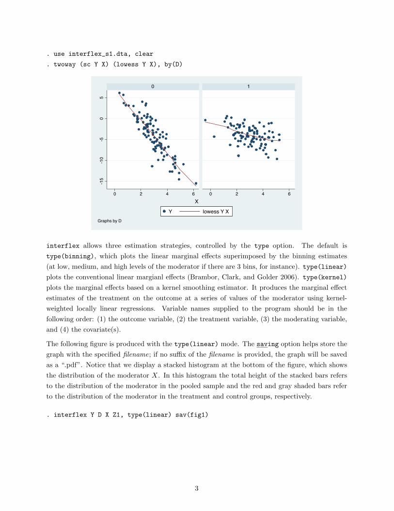
. use interflex_s1.dta, clear

. twoway (sc Y X) (lowess Y X), by(D)

-15

-10

-50

5

0 2 4 6 0 2 4 6

0 1

Y lowess Y X

X

Graphs by D

interflex allows three estimation strategies, controlled by the type option. The default is

type(binning), which plots the linear marginal effects superimposed by the binning estimates

(at low, medium, and high levels of the moderator if there are 3 bins, for instance). type(linear)

plots the conventional linear margianl effects (Brambor, Clark, and Golder 2006). type(kernel)

plots the marginal effects based on a kernel smoothing estimator. It produces the marginal effect

estimates of the treatment on the outcome at a series of values of the moderator using kernel-

weighted locally linear regressions. Variable names supplied to the program should be in the

following order: (1) the outcome variable, (2) the treatment variable, (3) the moderating variable,

and (4) the covariate(s).

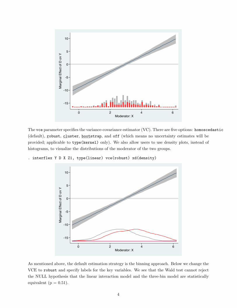
The following figure is produced with the type(linear) mode. The saving option helps store the

graph with the specified filename; if no suffix of the filename is provided, the graph will be saved

as a “.pdf”. Notice that we display a stacked histogram at the bottom of the figure, which shows

the distribution of the moderator X. In this histogram the total height of the stacked bars refers

to the distribution of the moderator in the pooled sample and the red and gray shaded bars refer

to the distribution of the moderator in the treatment and control groups, respectively.

. interflex Y D X Z1, type(linear) sav(fig1)

3

-15

-10

-5

0

5

10

Mar

gina

l Effe

ct o

f D o

n Y

0 2 4 6Moderator: X

The vce parameter specifies the variance-covariance estimator (VC). There are five options: homoscedastic

(default), robust, cluster, bootstrap, and off (which means no uncertainty estimates will be

provided; applicable to type(kernel) only). We also allow users to use density plots, instead of

histograms, to visualize the distributions of the moderator of the two groups.

. interflex Y D X Z1, type(linear) vce(robust) xd(density)

-15

-10

-5

0

5

10

Mar

gina

l Effe

ct o

f D o

n Y

0 2 4 6Moderator: X

As mentioned above, the default estimation strategy is the binning approach. Below we change the

VCE to robust and specify labels for the key variables. We see that the Wald test cannot reject

the NULL hypothesis that the linear interaction model and the three-bin model are statistically

equivalent (p = 0.51).

4

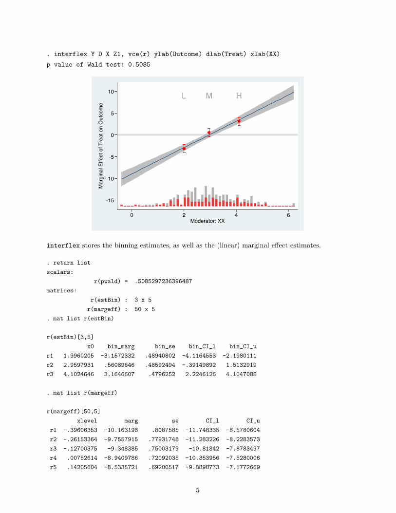
. interflex Y D X Z1, vce(r) ylab(Outcome) dlab(Treat) xlab(XX)

p value of Wald test: 0.5085

L M H

-15

-10

-5

0

5

10M

argi

nal E

ffect

of T

reat

on

Out

com

e

0 2 4 6Moderator: XX

interflex stores the binning estimates, as well as the (linear) marginal effect estimates.

. return list

scalars:

r(pwald) = .5085297236396487

matrices:

r(estBin) : 3 x 5

r(margeff) : 50 x 5

. mat list r(estBin)

r(estBin)[3,5]

x0 bin_marg bin_se bin_CI_l bin_CI_u

r1 1.9960205 -3.1572332 .48940802 -4.1164553 -2.1980111

r2 2.9597931 .56089646 .48592494 -.39149892 1.5132919

r3 4.1024646 3.1646607 .4796252 2.2246126 4.1047088

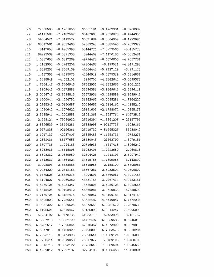
. mat list r(margeff)

r(margeff)[50,5]

xlevel marg se CI_l CI_u

r1 -.39606353 -10.163198 .8087585 -11.748335 -8.5780604

r2 -.26153364 -9.7557915 .77931748 -11.283226 -8.2283573

r3 -.12700375 -9.348385 .75003179 -10.81842 -7.8783497

r4 .00752614 -8.9409786 .72092035 -10.353956 -7.5280006

r5 .14205604 -8.5335721 .69200517 -9.8898773 -7.1772669

5

r6 .27658593 -8.1261656 .66331191 -9.4262331 -6.8260982

r7 .41111582 -7.7187592 .63487065 -8.9630828 -6.4744356

r8 .54564571 -7.3113527 .60671684 -8.5004959 -6.1222096

r9 .68017561 -6.9039463 .57889243 -8.0385546 -5.7693379

r10 .8147055 -6.4965398 .55144726 -7.5773566 -5.415723

r11 .94923539 -6.0891333 .5244409 -7.1170186 -5.0612481

r12 1.0837653 -5.6817269 .49794473 -6.6576806 -4.7057731

r13 1.2182952 -5.2743204 .47204468 -6.199511 -4.3491298

r14 1.3528251 -4.8669139 .44684442 -5.7427129 -3.991115

r15 1.487355 -4.4595075 .42246919 -5.2875319 -3.6314831

r16 1.6218849 -4.052101 .3990702 -4.8342642 -3.2699378

r17 1.7564147 -3.6446946 .37682936 -4.3832665 -2.9061226

r18 1.8909446 -3.2372881 .35596381 -3.9349643 -2.5396119

r19 2.0254745 -2.8298816 .33672931 -3.4898589 -2.1699043

r20 2.1600044 -2.4224752 .31942065 -3.0485281 -1.7964222

r21 2.2945343 -2.0150687 .30436655 -2.6116162 -1.4185212

r22 2.4290642 -1.6076622 .29191605 -2.1798072 -1.0355173

r23 2.5635941 -1.2002558 .28241368 -1.7537764 -.64673515

r24 2.698124 -.79284932 .27616394 -1.3341207 -.25157795

r25 2.8326539 -.38544286 .27338998 -.92127737 .15039166

r26 2.9671838 .02196361 .27419732 -.51545327 .55938049

r27 3.1017137 .42937007 .27855483 -.11658736 .9753275

r28 3.2362436 .83677653 .28630043 .27563799 1.3979151

r29 3.3707735 1.244183 .29716933 .6617418 1.8266242

r30 3.5053033 1.6515895 .31083406 1.0423659 2.260813

r31 3.6398332 2.0589959 .32694426 1.418197 2.6997949

r32 3.7743631 2.4664024 .34515765 1.7899058 3.142899

r33 3.908893 2.8738088 .36515968 2.158109 3.5895087

r34 4.0434229 3.2812153 .38667287 2.5233504 4.0390802

r35 4.1779528 3.6886218 .4094591 2.8860967 4.4911468

r36 4.3124827 4.0960282 .43331758 3.2467414 4.9453151

r37 4.4470126 4.5034347 .4580808 3.6056128 5.4012566

r38 4.5815425 4.9108412 .48360981 3.9629833 5.858699

r39 4.7160724 5.3182476 .50978957 4.3190784 6.3174168

r40 4.8506023 5.7256541 .53652482 4.6740847 6.7772234

r41 4.9851322 6.1330605 .56373655 5.0281572 7.2379639

r42 5.1196621 6.540467 .59135898 5.3814247 7.6995093

r43 5.254192 6.9478735 .61933715 5.733995 8.161752

r44 5.3887218 7.3552799 .64762497 6.0859583 8.6246015

r45 5.5232517 7.7626864 .67618357 6.4373909 9.0879818

r46 5.6577816 8.1700929 .70498005 6.7883573 9.5518284

r47 5.7923115 8.5774993 .73398641 7.1389124 10.016086

r48 5.9268414 8.9849058 .76317872 7.489103 10.480709

r49 6.0613713 9.3923122 .79253643 7.8389694 10.945655

r50 6.1959012 9.7997187 .82204183 8.1885463 11.410891

6

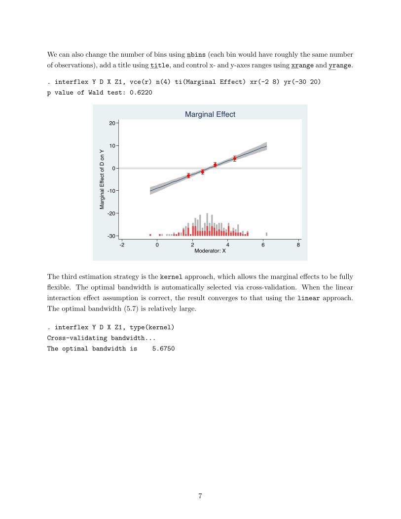
We can also change the number of bins using nbins (each bin would have roughly the same number

of observations), add a title using title, and control x- and y-axes ranges using xrange and yrange.

. interflex Y D X Z1, vce(r) n(4) ti(Marginal Effect) xr(-2 8) yr(-30 20)

p value of Wald test: 0.6220

-30

-20

-10

0

10

20

Mar

gina

l Effe

ct o

f D o

n Y

-2 0 2 4 6 8Moderator: X

Marginal Effect

The third estimation strategy is the kernel approach, which allows the marginal effects to be fully

flexible. The optimal bandwidth is automatically selected via cross-validation. When the linear

interaction effect assumption is correct, the result converges to that using the linear approach.

The optimal bandwidth (5.7) is relatively large.

. interflex Y D X Z1, type(kernel)

Cross-validating bandwidth...

The optimal bandwidth is 5.6750

7

-15

-10

-5

0

5

10

Mar

gina

l Effe

ct o

f D o

n Y

0 2 4 6Moderator: X

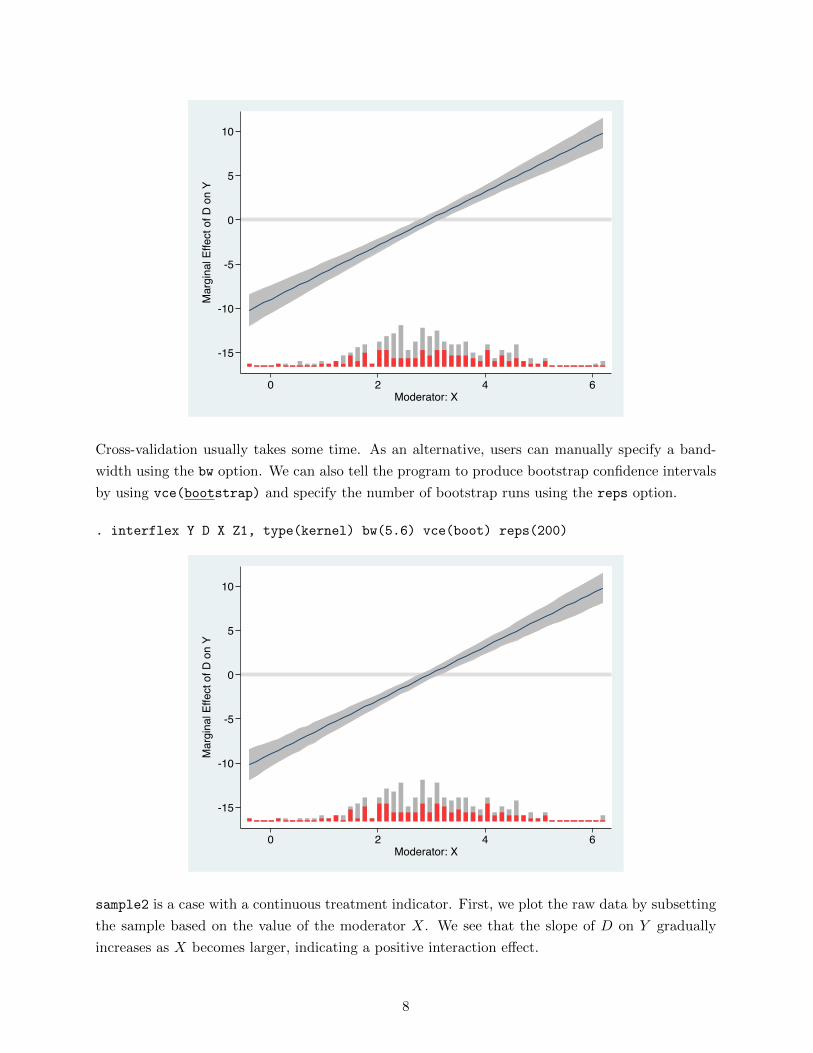
Cross-validation usually takes some time. As an alternative, users can manually specify a band-

width using the bw option. We can also tell the program to produce bootstrap confidence intervals

by using vce(bootstrap) and specify the number of bootstrap runs using the reps option.

. interflex Y D X Z1, type(kernel) bw(5.6) vce(boot) reps(200)

-15

-10

-5

0

5

10

Mar

gina

l Effe

ct o

f D o

n Y

0 2 4 6Moderator: X

sample2 is a case with a continuous treatment indicator. First, we plot the raw data by subsetting

the sample based on the value of the moderator X. We see that the slope of D on Y gradually

increases as X becomes larger, indicating a positive interaction effect.

8

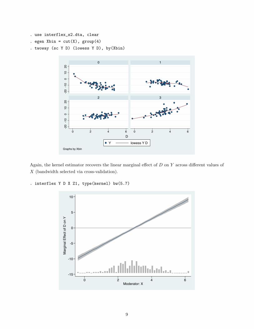
. use interflex_s2.dta, clear

. egen Xbin = cut(X), group(4)

. twoway (sc Y D) (lowess Y D), by(Xbin)

-20

-10

010

20-2

0-1

00

1020

0 2 4 6 0 2 4 6

0 1

2 3

Y lowess Y D

D

Graphs by Xbin

Again, the kernel estimator recovers the linear marginal effect of D on Y across different values of

X (bandwidth selected via cross-validation).

. interflex Y D X Z1, type(kernel) bw(5.7)

-15

-10

-5

0

5

10

Mar

gina

l Effe

ct o

f D o

n Y

0 2 4 6Moderator: X

9

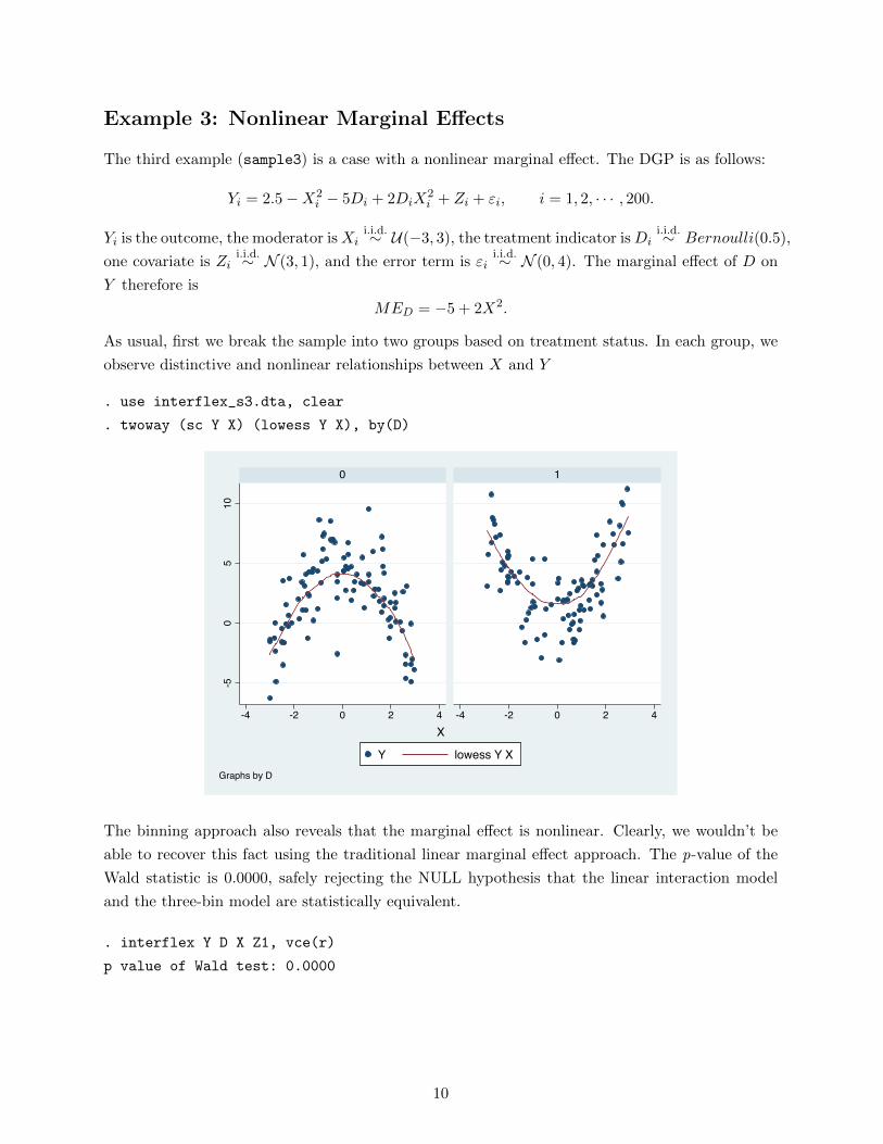
Example 3: Nonlinear Marginal Effects

The third example (sample3) is a case with a nonlinear marginal effect. The DGP is as follows:

Yi = 2.5−X2i − 5Di + 2DiX

2i + Zi + εi, i = 1, 2, · · · , 200.

Yi is the outcome, the moderator isXii.i.d.∼ U(−3, 3), the treatment indicator isDi

i.i.d.∼ Bernoulli(0.5),

one covariate is Zii.i.d.∼ N (3, 1), and the error term is εi

i.i.d.∼ N (0, 4). The marginal effect of D on

Y therefore is

MED = −5 + 2X2.

As usual, first we break the sample into two groups based on treatment status. In each group, we

observe distinctive and nonlinear relationships between X and Y

. use interflex_s3.dta, clear

. twoway (sc Y X) (lowess Y X), by(D)

-50

510

-4 -2 0 2 4 -4 -2 0 2 4

0 1

Y lowess Y X

X

Graphs by D

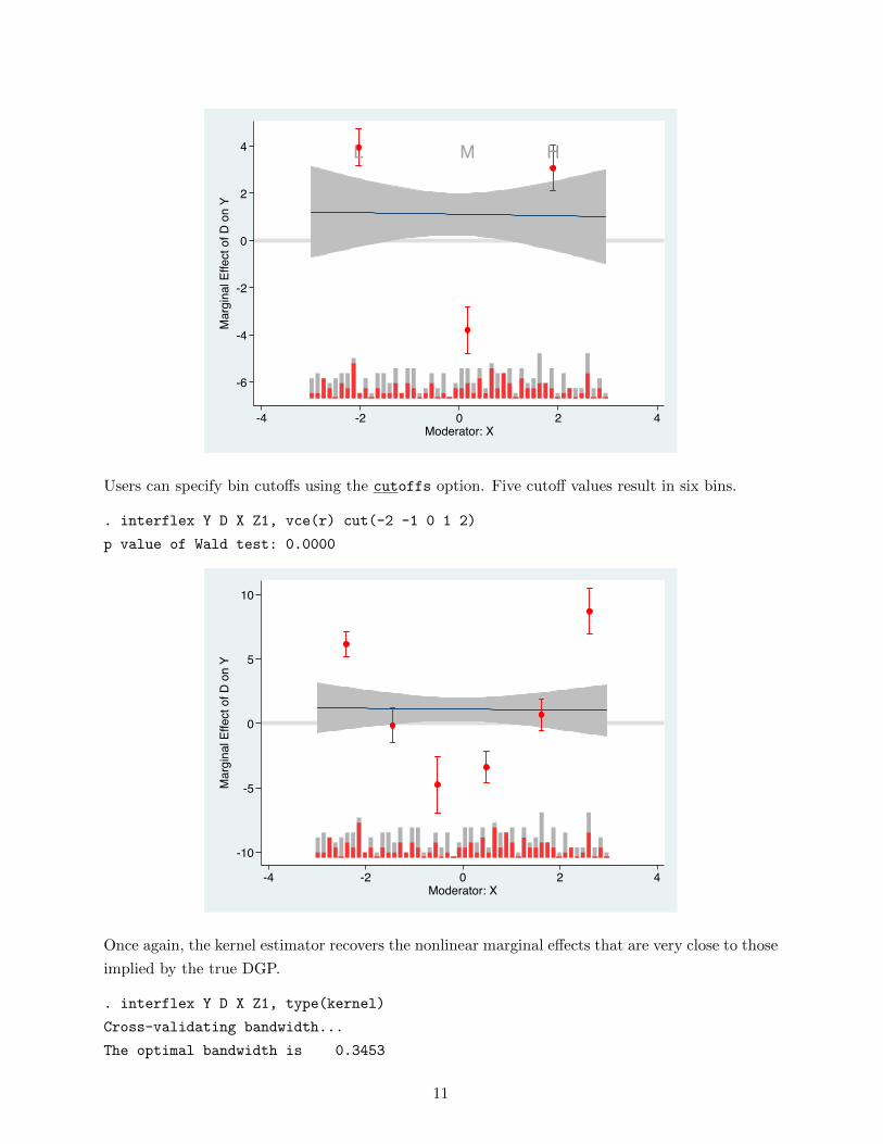
The binning approach also reveals that the marginal effect is nonlinear. Clearly, we wouldn’t be

able to recover this fact using the traditional linear marginal effect approach. The p-value of the

Wald statistic is 0.0000, safely rejecting the NULL hypothesis that the linear interaction model

and the three-bin model are statistically equivalent.

. interflex Y D X Z1, vce(r)

p value of Wald test: 0.0000

10

L M H

-6

-4

-2

0

2

4

Mar

gina

l Effe

ct o

f D o

n Y

-4 -2 0 2 4Moderator: X

Users can specify bin cutoffs using the cutoffs option. Five cutoff values result in six bins.

. interflex Y D X Z1, vce(r) cut(-2 -1 0 1 2)

p value of Wald test: 0.0000

-10

-5

0

5

10

Mar

gina

l Effe

ct o

f D o

n Y

-4 -2 0 2 4Moderator: X

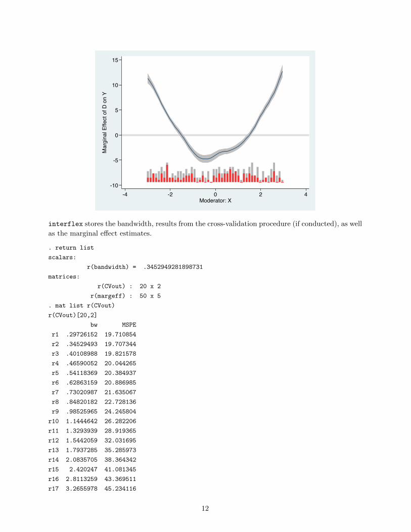
Once again, the kernel estimator recovers the nonlinear marginal effects that are very close to those

implied by the true DGP.

. interflex Y D X Z1, type(kernel)

Cross-validating bandwidth...

The optimal bandwidth is 0.3453

11

-10

-5

0

5

10

15

Mar

gina

l Effe

ct o

f D o

n Y

-4 -2 0 2 4Moderator: X

interflex stores the bandwidth, results from the cross-validation procedure (if conducted), as well

as the marginal effect estimates.

. return list

scalars:

r(bandwidth) = .3452949281898731

matrices:

r(CVout) : 20 x 2

r(margeff) : 50 x 5

. mat list r(CVout)

r(CVout)[20,2]

bw MSPE

r1 .29726152 19.710854

r2 .34529493 19.707344

r3 .40108988 19.821578

r4 .46590052 20.044265

r5 .54118369 20.384937

r6 .62863159 20.886985

r7 .73020987 21.635067

r8 .84820182 22.728136

r9 .98525965 24.245804

r10 1.1444642 26.282206

r11 1.3293939 28.919365

r12 1.5442059 32.031695

r13 1.7937285 35.285973

r14 2.0835705 38.364342

r15 2.420247 41.081345

r16 2.8113259 43.369511

r17 3.2655978 45.234116

12

r18 3.7932738 46.717565

r19 4.4062151 47.876913

r20 5.1181993 48.770929

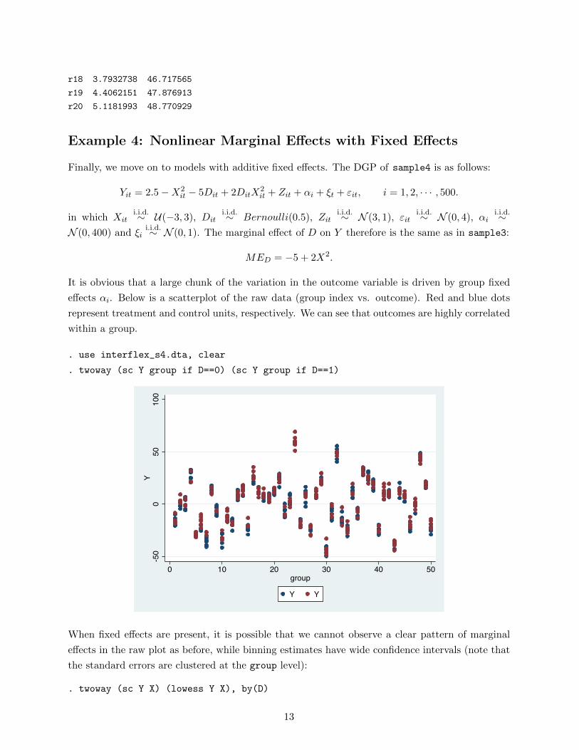
Example 4: Nonlinear Marginal Effects with Fixed Effects

Finally, we move on to models with additive fixed effects. The DGP of sample4 is as follows:

Yit = 2.5−X2it − 5Dit + 2DitX

2it + Zit + αi + ξt + εit, i = 1, 2, · · · , 500.

in which Xiti.i.d.∼ U(−3, 3), Dit

i.i.d.∼ Bernoulli(0.5), Ziti.i.d.∼ N (3, 1), εit

i.i.d.∼ N (0, 4), αii.i.d.∼

N (0, 400) and ξii.i.d.∼ N (0, 1). The marginal effect of D on Y therefore is the same as in sample3:

MED = −5 + 2X2.

It is obvious that a large chunk of the variation in the outcome variable is driven by group fixed

effects αi. Below is a scatterplot of the raw data (group index vs. outcome). Red and blue dots

represent treatment and control units, respectively. We can see that outcomes are highly correlated

within a group.

. use interflex_s4.dta, clear

. twoway (sc Y group if D==0) (sc Y group if D==1)

-50

050

100

Y

0 10 20 30 40 50group

Y Y

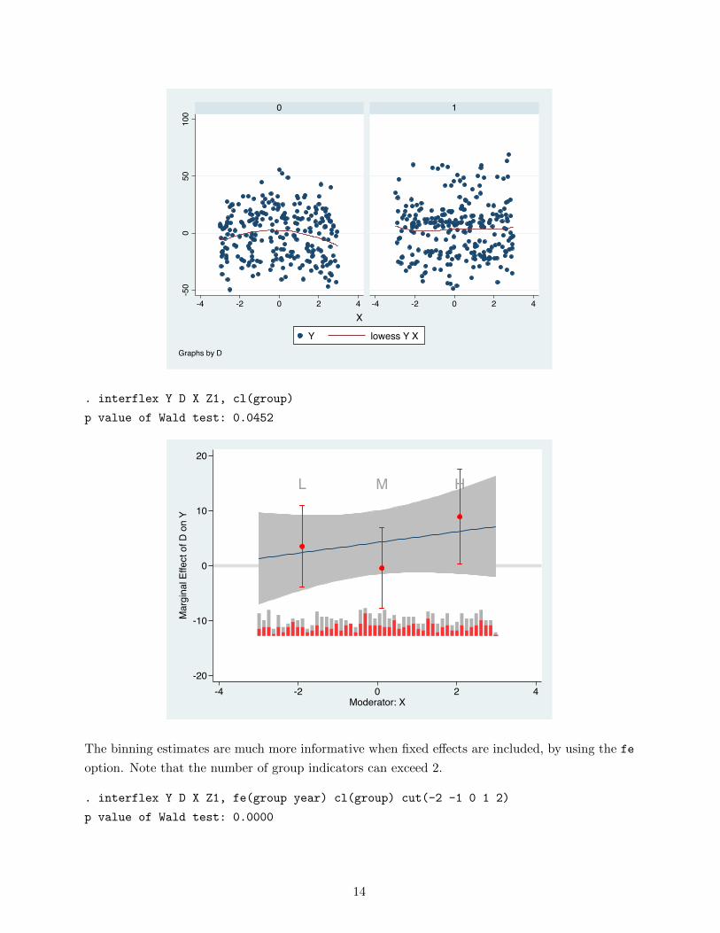
When fixed effects are present, it is possible that we cannot observe a clear pattern of marginal

effects in the raw plot as before, while binning estimates have wide confidence intervals (note that

the standard errors are clustered at the group level):

. twoway (sc Y X) (lowess Y X), by(D)

13

-50

050

100

-4 -2 0 2 4 -4 -2 0 2 4

0 1

Y lowess Y X

X

Graphs by D

. interflex Y D X Z1, cl(group)

p value of Wald test: 0.0452

L M H

-20

-10

0

10

20

Mar

gina

l Effe

ct o

f D o

n Y

-4 -2 0 2 4Moderator: X

The binning estimates are much more informative when fixed effects are included, by using the fe

option. Note that the number of group indicators can exceed 2.

. interflex Y D X Z1, fe(group year) cl(group) cut(-2 -1 0 1 2)

p value of Wald test: 0.0000

14

-10

-5

0

5

10

Mar

gina

l Effe

ct o

f D o

n Y

-4 -2 0 2 4Moderator: X

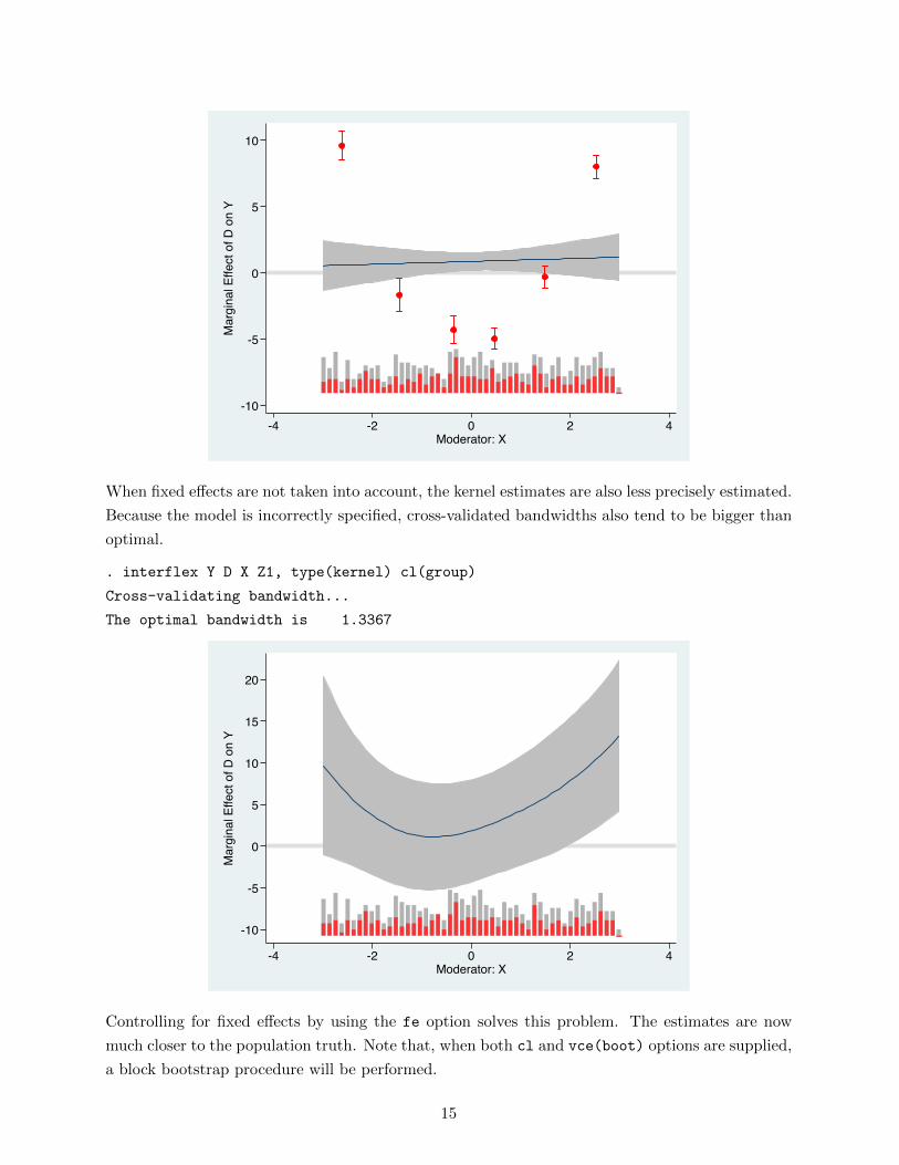
When fixed effects are not taken into account, the kernel estimates are also less precisely estimated.

Because the model is incorrectly specified, cross-validated bandwidths also tend to be bigger than

optimal.

. interflex Y D X Z1, type(kernel) cl(group)

Cross-validating bandwidth...

The optimal bandwidth is 1.3367

-10

-5

0

5

10

15

20

Mar

gina

l Effe

ct o

f D o

n Y

-4 -2 0 2 4Moderator: X

Controlling for fixed effects by using the fe option solves this problem. The estimates are now

much closer to the population truth. Note that, when both cl and vce(boot) options are supplied,

a block bootstrap procedure will be performed.

15

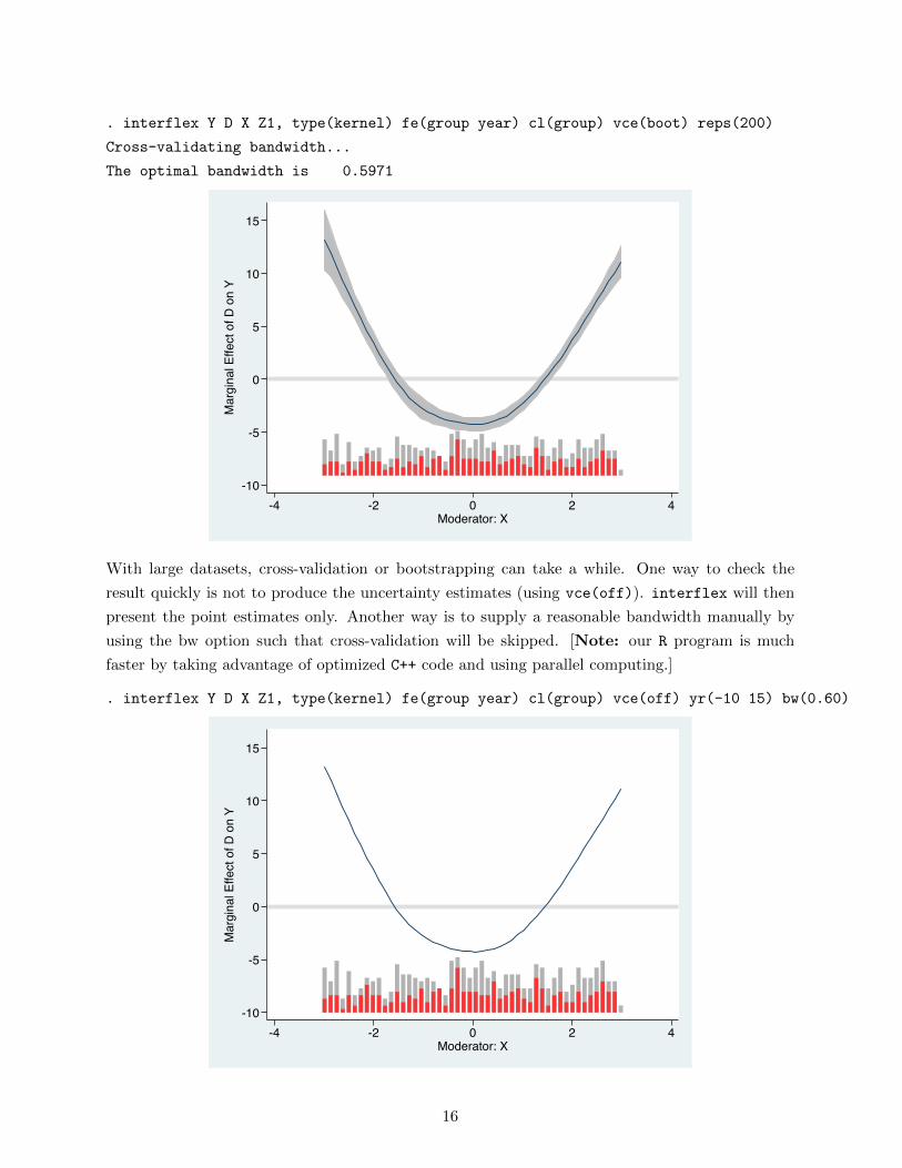
. interflex Y D X Z1, type(kernel) fe(group year) cl(group) vce(boot) reps(200)

Cross-validating bandwidth...

The optimal bandwidth is 0.5971

-10

-5

0

5

10

15M

argi

nal E

ffect

of D

on

Y

-4 -2 0 2 4Moderator: X

With large datasets, cross-validation or bootstrapping can take a while. One way to check the

result quickly is not to produce the uncertainty estimates (using vce(off)). interflex will then

present the point estimates only. Another way is to supply a reasonable bandwidth manually by

using the bw option such that cross-validation will be skipped. [Note: our R program is much

faster by taking advantage of optimized C++ code and using parallel computing.]

. interflex Y D X Z1, type(kernel) fe(group year) cl(group) vce(off) yr(-10 15) bw(0.60)

-10

-5

0

5

10

15

Mar

gina

l Effe

ct o

f D o

n Y

-4 -2 0 2 4Moderator: X

16