Reservoir-geological Characterization of a Fractured Limestone ...

User guide of reservoir geological modeling
1 Quick Look
1.1 Introduction
On the basis of structural model, reservoir geological modeling is used for generating
reservoir geological grid, then filling the cells of the grid with discrete (facies and lithology)
or continuous (porosity, permeability, and saturation, etc.) properties by using geo-statistical
method.
1.2 Module relationships
In order to carry out reservoir geological modeling, it must be built on the basis of the
structural model, meanwhile it provides the basic data for numerical simulation gridding. This
module also provides vector data to plan and profile module.
Fig. 1-1 Relationships between Reservoir geological modeling module and others.

1.3 General workflow
Fig.1‐2Reservoir geometrical modeling workflow.
Property modeling is divided into three separate processes:
1.3.1 Reservoir geometrical modeling
Truncated rectangular grid as the reservoir geological grid can accurately describe any
complex structural model.
Fig.1‐3Truncated rectangular grid for structural model.
1.3.2 Facies modeling
Interpolation or simulation of discrete data, for example, facies.
1.3.3 Petrophysical modeling
Interpolation or simulation of continuous data, for example, porosity, permeability, and
saturation:
1) Firstly, choose the interested zones to generate the reservoir geological model;

2) Then, generate reservoir geological grid based on the structural model. Both in the facies
and petrophysical model, creating property body is necessary, and the data are stored in it;
3) After that, extract well logs, scale up the logs and do data analysis (including Convert and
Variogram);
4) Finally, simulate using deterministic or stochastic algorithm according to a series of
geological statistics method.

2 How to model a reservoir geological model
2.1 Node meaning
Reservoir Geological Modeling Module can manage multiple reservoir geological models,
which had different specifications of horizons and grids at the same time.
Node meaning in a reservoir geological model:
Fig. 2-1 Nodes in the tree pane.
①Model node: manage Horizons, Sections and Properties nodes.
②Horizons node: manage more stratums which belongs to Horizons (Type: Horizon)) in
Structural Modeling Module.
③Horizon node: manage one stratum which belongs to Horizons (Type: Horizon) in
Structural Modeling Module.
④Horizon (well tops) node: manage more stratums which belongs to Horizons (Type:
Horizon (well tops)) in Structural Modeling Module.
⑤Property body node: manage the display of 3D geo-cellar grids, the results of upscaling
and surfaces of simulated result. Store the results of upscaling and interpolation simulation.
Support multiple implementation.
⑥Sections node: manage a series of general sections.

⑦Properties node: manage various kinds of discrete and continuous properties. Each
property exist independently, has its own grid specifications, the data source and colors, etc.
⑧Property node: a discrete or continuous properties, manage the display of solid model.
2.2 Reservoir geometrical modeling
2.2.1 Modeling preparation
A structural model of depth-domain.
2.2.2 Operation process
Fig. 2-2 Reservoir geometrical modeling workflow.
1) Create new model
(1) Right click in the Tree Pane and select New model.
Fig. 2-3 Create new model.
(2) Set a model name and select the interested zones in the pop-up dialog.

Fig. 2-4 Choose interested zones.
Note: Double-click left button to select the first zone, double-click right button to select the
last zone. The zones marked red will be used in this reservoir model.
2) Define model boundary
(1) Right click on the new reservoir model and select Define model of boundary.
Fig. 2-5 Define model boundary.
Three methods can be used when defining model boundary:
Draw: artificial drawing
Set: artificial set coordinates
Fig. 2-6 Set artificial coordinates.
Import: import boundary coordinates file

Fig. 2-7 Import boundary coordinates file.
3) Generate 3D geo-cellar grids
Right click on the new reservoir model and select Generate model.
Fig. 2-8 Generate geo-cellar grids.
Truncated rectangular grid as the reservoir geological grid can accurately describe any
complex structural model.
Fig. 2-9 Truncated rectangular grid generation process.
Note: A structural model of Depth-domain has been created before making reservoir model.
2.3 Facies modeling
2.3.1 Modeling preparation
Generated 3D geo-cellar grids, well logs (discrete data) or facies map (.DFD format).
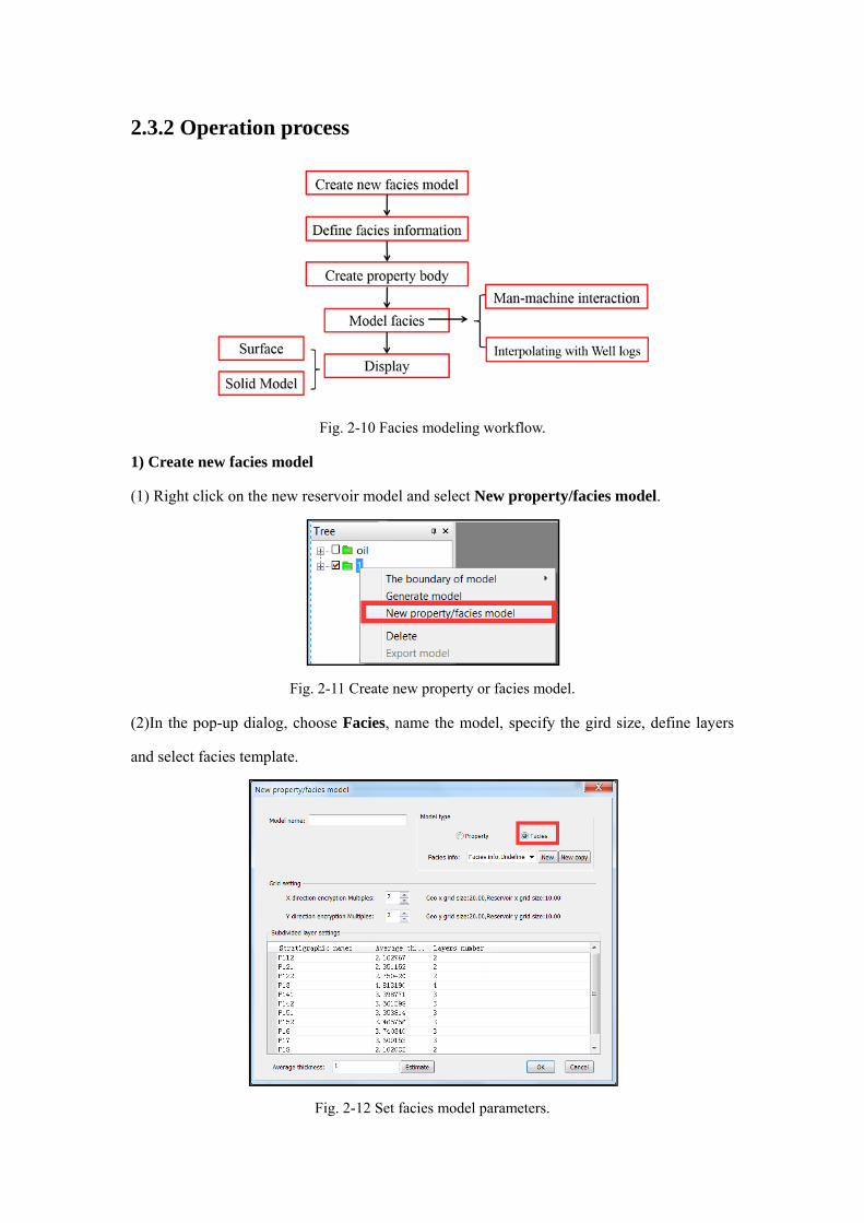
2.3.2 Operation process
Fig. 2-10 Facies modeling workflow.
1) Create new facies model
(1) Right click on the new reservoir model and select New property/facies model.
Fig. 2-11 Create new property or facies model.
(2)In the pop-up dialog, choose Facies, name the model, specify the gird size, define layers
and select facies template.
Fig. 2-12 Set facies model parameters.

Note: layers can be defined by specifying a number for average thickness and then clicking
estimate or directly specifying a number for layers number. For Facies Info, either selecting a
default one or creating a new one is feasible.
2) Define facies information
(1) Right click on the new facies model and select Edit faices information.
Fig. 2-13 Choose Edit facies information.
(2) In the pop-up dialog, right click in the blank and select Insert phase, and then name it.
Switch to Table editing mode, assign colors to different facies.
Fig. 2-14 Edit facies information in pop-up dialog
Note: facies code is automatically created when a new phase is inserted. It is an internal
information in the process of making facies.

Fig. 2-15 Set facies colors corresponding to maps.
Note: must make sure the facies have identical color with provided maps (.DFD) when
assigning colors. For example, RGB values, the expression of color.
Fig. 2-16 Keep facies name consistent with the number of name on well logs.
Note: it is necessary that the facies name must be kept consistent with the number or name in
the well logs.
3) Create property body
Right click Oil layer group and select Create property body.
Fig. 2-17 Create property body.
Note: as the carrier of modeling, it is necessary to create property body before assigning
values or interpolating data

4) Man-machine interaction (the first method for facies modeling)
(1) Right click Oil layer group and select Batched import facies maps of DFD format or
right click the name any zone and select Import the facies map of DFD format.
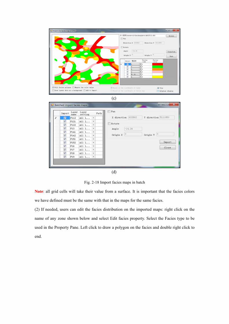
Fig. 2-18 Import facies maps in batch
Note: all grid cells will take their value from a surface. It is important that the facies colors
we have defined must be the same with that in the maps for the same facies.
(2) If needed, users can edit the facies distribution on the imported maps: right click on the
name of any zone shown below and select Edit facies property. Select the Facies type to be
used in the Property Pane. Left click to draw a polygon on the facies and double right click to
end.

Fig. 2-19 Edit facies property manually.
Note: if there is no facies map, user can edit facies distribution directly based on the
geological recognition of the model.
5) Interpolating with well logs (the second method for facies modeling)
Fig. 2-20 Interpolating with well logs.
(1) Import well logs
Click the activated model, in its Property Pane specify the Data sources as well logs, and
then in the pull-down menu select the corresponding log.
Right click Oil layer group and select Extract well logs.
Fig. 2-21 Select data sources in property pane.

Fig. 2-22 Extract well logs in tree pane.
(2) Scale up well logs
Right click on the name any zone and select Scale up or right click on Oil layer group and
select Scale up.
Fig. 2-23 Scale up well longs.
In the pop-up dialog, specify the settings to scale up the discrete log.
The following methods for Scale up well logs are available: Most of, Median, Minimum,
Maximum, Arithmetic average, Mid point pick, Random pick.
Detailed see Methods in Scale up well logs.
Fig. 2-24 Scale up setting dialog box.

(3) Data analysis
Right click on the name of any zone and select Data analysis.
Fig. 2-25 Data analysis in tree pane.
In the settings tab of a data object, inspect the property distributions and the correlation
between properties.
Fig. 2-26 Data Analysis dialog box.
①Config: Save the results of parameters setting. A variety of different parameters
configuration tables can be saved.
②The name of facies model.
③Horizon name.
④Variogram tab:generate a discrete variograms to describe the facies distribution. Detailed
see Variogram tab in Continuous data analysis.

⑤Hint: Copyright statement about using the algorithm.
Note: DepthInsight® software directly uses the interpolation algorithm of GSLIB library to
simulate, then updates the results to the reservoir geometrical grid.
(4) Data interpolation
Right click the name of any zone and select Data interpolation.
Fig. 2-27 Select Data interpolation in tree pane.
Using deterministic or stochastic geo-statistics algorithms, the discrete properties are
simulated within the reservoir geological cells.
Fig. 2-28 Select interpolation methds in Data interpolation dialog box.
The following methods for Data interpolation are available: Sequential Indicator
Simulation (SIS) and Indicator Kriging.
Detailed see Sequential Indicator Simulation (SIS) and Indicator Kriging in Simulation
methods.
In the pop-up dialog, facies control and second variable are available.
Facies control: use existing layer property of facies model to control and assist modeling.
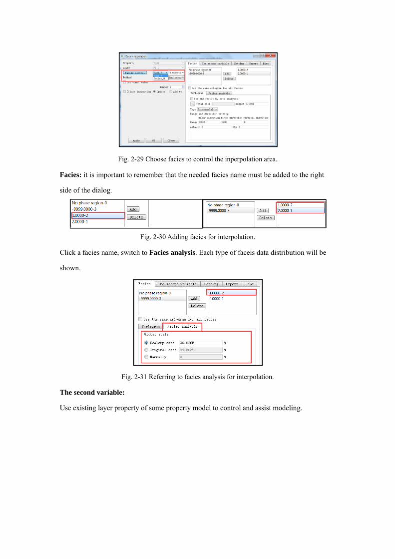
Fig. 2-29 Choose facies to control the inperpolation area.
Facies: it is important to remember that the needed facies name must be added to the right
side of the dialog.
Fig. 2-30 Adding facies for interpolation.
Click a facies name, switch to Facies analysis. Each type of faceis data distribution will be
shown.
Fig. 2-31 Referring to facies analysis for interpolation.
The second variable:
Use existing layer property of some property model to control and assist modeling.
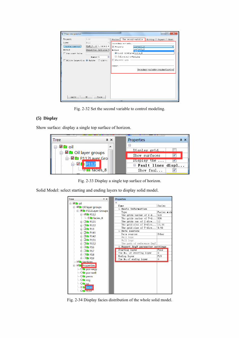
Fig. 2-32 Set the second variable to control modeling.
(5) Display
Show surface: display a single top surface of horizon.
Fig. 2-33 Display a single top surface of horizon.
Solid Model: select starting and ending layers to display solid model.
Fig. 2-34 Display facies distribution of the whole solid model.

2.4 Petrophysical modeling
2.4.1 Modeling preparation
Generated 3D geo-cellar grids, well logs (continuous data).
2.4.2 Operation process
Fig. 2-35 Petrophysical modeling workflow.
1) Create petrophysical model
Right click on the new reservoir model and select New property/facies model.
Fig. 2-36 Create a new property model.
In the pop-up dialog, choose Property, name the model, specify the gird size, define layers.
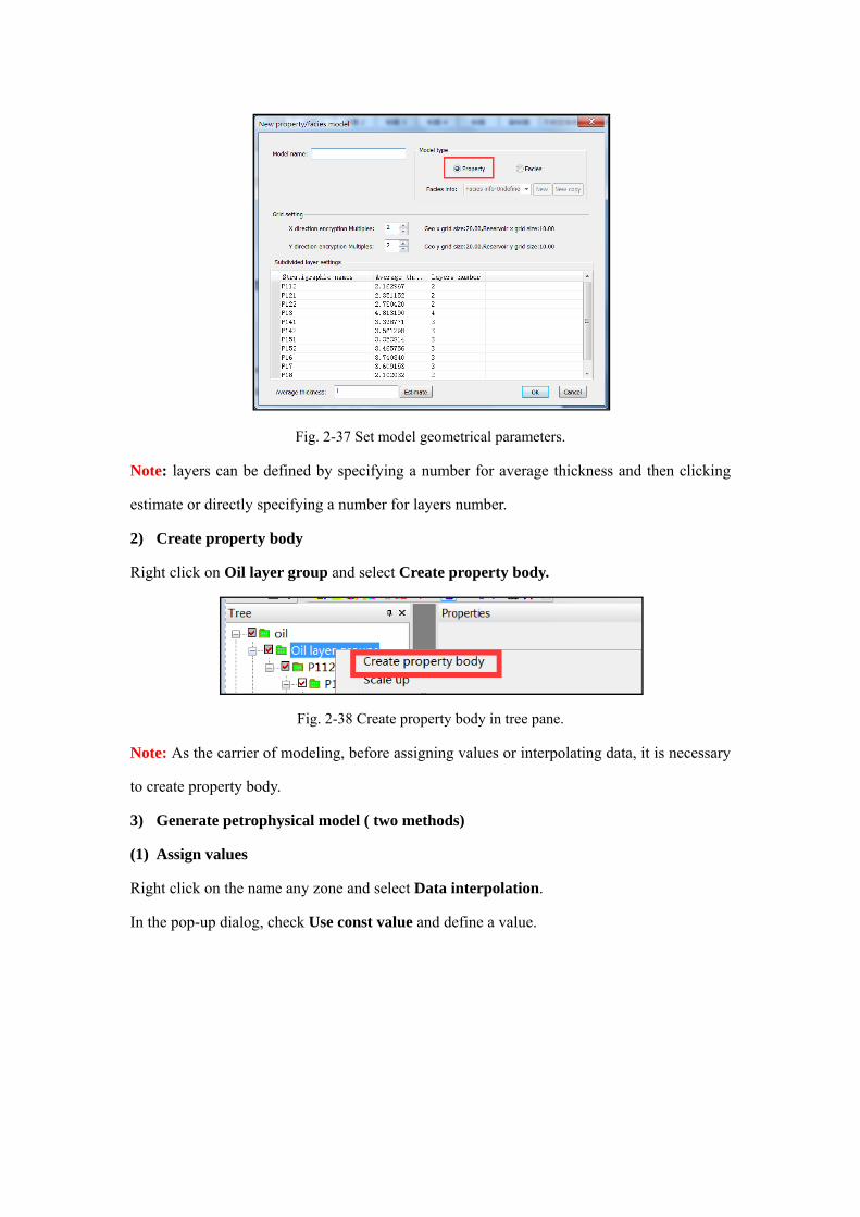
Fig. 2-37 Set model geometrical parameters.
Note: layers can be defined by specifying a number for average thickness and then clicking
estimate or directly specifying a number for layers number.
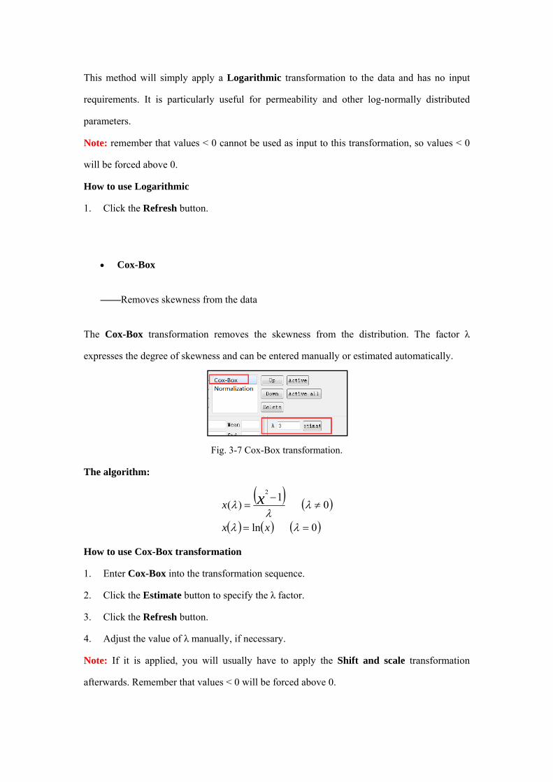
2) Create property body
Right click on Oil layer group and select Create property body.
Fig. 2-38 Create property body in tree pane.
Note: As the carrier of modeling, before assigning values or interpolating data, it is necessary
to create property body.
3) Generate petrophysical model ( two methods)
(1) Assign values
Right click on the name any zone and select Data interpolation.
In the pop-up dialog, check Use const value and define a value.

Fig. 2-39 Set constant value for property body.
Note: All grid cells will be given the same constant value.
(2) Interpolating with well logs
Import well logs
Click the activated model, in its Property Pane specify the Data sources as Well logs, and
then in the pull-down menu select the corresponding log.
Right click on Oil layer group and select Extract well logs.
Fig. 2-40 Set the data sources in property pane.
Fig. 2-41 Extract well logs for the created property body.
Scale up well logs
Right click on the name any zone and select Scale up or right click on Oil layer group and
select Scale up.

Fig. 2-42 Scale up well logs.
In the pop-up dialog, specify the settings to scale up the chosen log.
The following methods for Scale up well logs are available: Arithmetic average,Harmonic
mean, Geometric mean, RMS, Median, Minimum, Maximum, Mid point pick, Random
pick.
Detailed see Methods in Scale up well logs.
Fig. 2-43 Available algorithms for up-scaling.
Data analysis
Right click on the name of any zone and select Data analysis.
Fig. 2-44 Data analysis for the chosen property body.
In the Settings tab of a data object, inspect the property distributions and the correlation
between properties.

Fig. 2-45 Data analysis tab introduction.
①Config: Save the results of parameters setting. A variety of different parameters
configuration tables can be saved.
②The name of facies model
③Horizon name
④Transformation tab: detailed see Transformation tab in Data analysis.
⑤Detailed see Histogram window in Data analysis.

Fig. 2-46 Variogram tab introduction.
Variogram tab: generate a discrete variogram to describe the distribution. Detailed see
Variogram tab in Data analysis.
Fig. 2-47 Hint tab introduction.

Hint: copyright statement about using the algorithm.
Data interpolation
Right click on the name any zone and select Data interpolation.
Fig. 2-48 Data interpolation of chosen property.
Using deterministic or stochastic geo-statistics algorithms, the continuous properties are
simulated within the reservoir geological cells.
The following methods for Data interpolation are available: Sequential Gaussian
simulation(SGS) , Kriging and so on.
Detailed see Sequential Gaussian Simulation (SGS) and Kriging in Simulation methods.
Fig. 2-49 Available interpolation methods for choosing.
Note: clicking Estimate in the Distributed pane is required before interpolating.

Fig. 2-50 Estimate output parameter setting values before interpolating.
In the pop-up dialog, facies control and second variable are available.
Facies control
Use existing layer property of facies model to control and assist modeling.
Fig. 2-51 Set facies to control modeling.
The second variable
Use existing layer property of some property models (as the second variable like seismic
attributes or other petrophysical model) to control and assist modeling.
Fig. 2-52 Set second parameter to control modeling.
4) Display
The same as Display in Facies modeling.

3 Appendix
3.1 Scale up well logs
When modeling different properties, the modeled area is divided up by generating a 3D grid.
Each grid cell has a single value for each property.
As the grid cells often are much larger than the sample density for well logs, well log data
must be scaled up before it can be entered into the grid. This process is also called blocking of
well logs.
Depending on whether logs are discrete (Facies model) or continuous (Petrophysical model),
different methods will be available within the Scale up process window.
Fig. 3-1 Available algorithms for facies modeling.
Fig. 3-2 Available algorithms for continuous modeling.
The following methods for Scale up well logs are available:
Most of (only available for discrete logs)

——Will select the discrete value which is most represented in the log for each particular
cell
Median(only available for discrete logs)
——Will sort the input values and select the center value.
Minimum
——Will sample the minimum value of the well log for the cell.
Maximum
——Will sample the maximum value of the well log for the cell.
Arithmetic average
——Typically used for properties such as porosity, saturation, and net/gross because
these are additive variables. The arithmetic mean is only correct for horizontal
permeability that is constant within each layer in the model. A varied permeability will be
get too high a value using arithmetic mean since it is the lower permeability values which
will have the greatest influence on the effective permeability.
Mid Point Pick
——Will pick the log value where the well is halfway through the cell. This is essentially
a random choice and is therefore more likely to give a property with the same distribution
of values as the original well log data.
Random Pick

——Picks a log point at random from anywhere within the cell. This random option
avoids the smoothing tendency of other methods and is, therefore, more likely to give a
property with the same distribution of values as the original well log data.
Harmonic mean
——Gives the effective vertical permeability if the reservoir is layered with constant
permeability in each layer. The harmonic mean works well with log normal distributions.
Used for permeability because it is sensitive to lower values.
Note: The method is not defined for negative values, only measurements with values
greater than zero can be used.
Geometric mean
——Is normally a good estimate for permeability if it has no spatial correlation and is log
normally distributed. The geometric mean is sensitive to lower values, which will have a
greater influence of results.
Note: The method is not defined for negative values, only measurements with values
greater than zero can be used.
RMS (Root Mean Squared)
——Will provide a strong bias towards high values

3.2 Data analysis
Data analysis is a process of quality controlling and exploring the data, identifying key
geological features, and preparing inputs for Facies and Petrophysical modeling.
Depending on whether a property is discrete (Facies model) or continuous (Petrophysical
model), different tools will be available within the Data analysis process window.
3.2.1 Discrete data analysis
Discrete data analysis for analyzing the facies proportion, and also create a variogram, is
available for Facies model.
Fig. 3-3 Data analysis for facies proportion.
3.2.2 Continuous data analysis
Continuous data analysis for defining data transformations and to generate variograms. Data
transformation enables the user to make the data stationary and standard normally distributed,
which are requirements of many of the standard geostatistical algorithms, is available for
Petrophysical model.

Fig. 3-4 Data analysis for petrophysical model.
①Config: Save the results of parameters setting. A variety of different parameters
configuration tables can be saved.
②The name of petrophysical model
③Horizon name
④Transformation tab
(1) Transformation tab
Why do a transformation?
A stationary distribution is a basic requirement for input data to most geostatistical algorithms.
Standard normal distribution is a requirement of the Gslib Sequential Gaussian Simulation
algorithm used for stochastic petrophysical simulation. The data must be transformed so that
it fits this criteria.
What is a Transformation?
A transformation is the preparation of a real data set into an internal data set that meets the
statistical requirements given by a chosen algorithm. It will make the data stationary and

standard normally distributed before the actual modeling process. Back-transformation will be
automatically performed in the exact reverse order of the modeling result to preserve the
spatial trends and original data distribution in the final result property.
Main objectives:
To remove spatial trends so that the data will be stationary;
To transform the data into Standard normal distribution (with a mean of 0 and standard
deviation of 1).
Functions:
Viewing the data distribution as histograms;
Making different data transformations such as Normalization.
Methods:
Input Truncation
——Truncate the input data
Fig. 3-5 Truncate the input data.
The first transformation to be applied is usually Input truncation. This transformation will
truncate the input distribution to get rid of data not to be represented in the final output. If
your input data contains values that are outside the actual physical boundaries of the property,
the data truncation can be used to remove these (Min and Max) values.
It provides two schemes to deal with outside the range of data points:
Use periphery value
Include low values at the specified minimum and vice versa
Discard

Ignore values above or below the maximum and minimum respectively.
How to use Input Truncation:
1. Define the Min and the Max values of the input distribution.
2. Click the Refresh button.
3. You can also use Estimate to extract the min and max value of the transformed data.
Output Truncation
——Truncate the output data after Petrophysical modeling
Fig. 3-6 Truncate the output data.
The Output truncation is the last step of the back-transformation of the data. Therefore, it
has no effect on the histogram within the data Transformation tab. The Output truncation will
be performed on the output realization. This transformation is applied to ensure that your
realization does not get values outside the desired range.
How to use Output Truncation
1. Define the Min and the Max values of the output distribution.
2. Click the Refresh button.
3. You can also use Estimate to extract the min and max value of the transformed data.
Logarithmic
——Logarithmic transformation
This method will simply apply a Logarithmic transformation to the data and has no input
requirements. It is particularly useful for permeability and other log-normally distributed
parameters.
Note: remember that values < 0 cannot be used as input to this transformation, so values < 0
will be forced above 0.
How to use Logarithmic
1. Click the Refresh button.
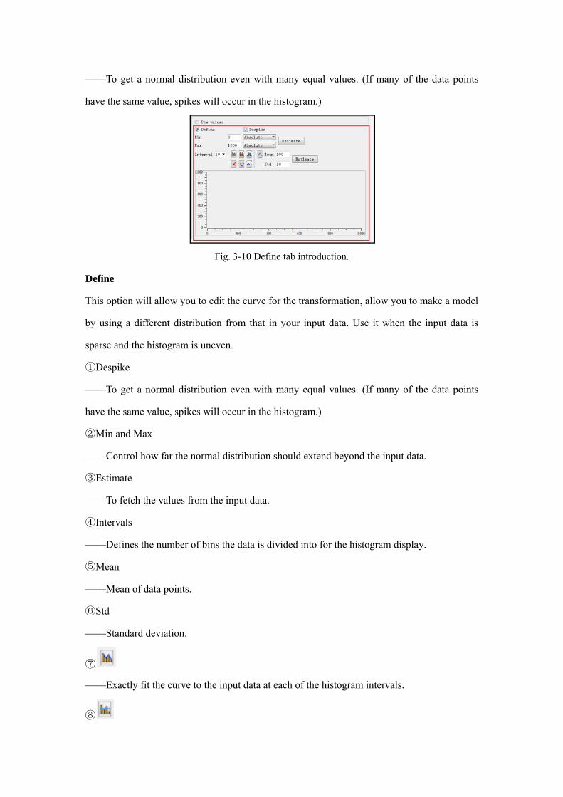
Cox-Box
——Removes skewness from the data
The Cox-Box transformation removes the skewness from the distribution. The factor λ
expresses the degree of skewness and can be entered manually or estimated automatically.
Fig. 3-7 Cox-Box transformation.
The algorithm:
0ln
01
)(2
xx
x x
How to use Cox-Box transformation
1. Enter Cox-Box into the transformation sequence.
2. Click the Estimate button to specify the λ factor.
3. Click the Refresh button.
4. Adjust the value of λ manually, if necessary.
Note: If it is applied, you will usually have to apply the Shift and scale transformation
afterwards. Remember that values < 0 will be forced above 0.

Shift and scale
——Shift the mean and scale the standard deviation of the data.
Fig. 3-8 Shift and scale transformation.
The Shift and scale transformation is used to shift and scale the data so that the mean is 0 and
the standard deviation is 1 and should usually be applied after any spatial transformations
(Cox-Box, Logarithmic). Unlike Normalization, it will not change the shape of the
distribution so the histogram should look like something close to a log normal distribution
before applying the transformation.
The algorithm:
deviationstd
meanvaluevaluedtransforme
_
)(_
The algorithm for Estimate:
n
meanxmeanxmeanxiance
n
xxxmean
n
n
222
21
21
)(...)()(var
...
How to use Shift and scale
1. Inspect the histogram after all other transformations have been applied (remember to
press the Refresh button to see the effect of the transformations). If the mean is different
from 0, then use the Shift and scale transformation
2. Include Shift and scale in the transformation list.

3. Click the Estimate button to get the Mean and the Std (standard deviations).
4. Click the Refresh button and inspect the changes.
Normalization
——Transform the data to a standard normal.
Normalization transformation will force any distribution to a standard normal distribution.
Normal distribution of data means that most of the samples in a set of data are close to the
Mean value, while relatively few samples tend to one extreme or the other. Normally
distributed data will have something like a "bell curve" shape.
Normalization transformations should be used with caution, particularly if you have limited
input data, as they will force the distribution of your property to exactly match the distribution
of your input, both the position and the relative height of the histogram bars. If the input data
is limited, then the histogram can be unrepresentative and will be matched exactly by the
distribution of the property modeling result.
There are two main options:
Fig. 3-9 Use values tab introduction.
Use values
This will base the transformation purely on your own data. Use it when you have a large
number of data points with a reasonable spread.
①Min and Max
——Control how far the normal distribution should extend beyond the input data.
②Estimate
——To get a reasonable value.
③Despike
——To get a normal distribution even with many equal values. (If many of the data points
have the same value, spikes will occur in the histogram.)
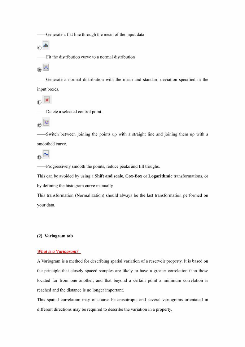
Fig. 3-10 Define tab introduction.
Define
This option will allow you to edit the curve for the transformation, allow you to make a model
by using a different distribution from that in your input data. Use it when the input data is
sparse and the histogram is uneven.
①Despike
——To get a normal distribution even with many equal values. (If many of the data points
have the same value, spikes will occur in the histogram.)
②Min and Max
——Control how far the normal distribution should extend beyond the input data.
③Estimate
——To fetch the values from the input data.
④Intervals
——Defines the number of bins the data is divided into for the histogram display.
⑤Mean
——Mean of data points.
⑥Std
——Standard deviation.
⑦
——Exactly fit the curve to the input data at each of the histogram intervals.
⑧
——Generate a flat line through the mean of the input data
⑨
——Fit the distribution curve to a normal distribution
⑩
——Generate a normal distribution with the mean and standard deviation specified in the
input boxes.
⑪
——Delete a selected control point.
⑫
——Switch between joining the points up with a straight line and joining them up with a
smoothed curve.
⑬
——Progressively smooth the points, reduce peaks and fill troughs.
This can be avoided by using a Shift and scale, Cox-Box or Logarithmic transformations, or
by defining the histogram curve manually.
This transformation (Normalization) should always be the last transformation performed on
your data.
(2) Variogram tab
What is a Variogram?
A Variogram is a method for describing spatial variation of a reservoir property. It is based on
the principle that closely spaced samples are likely to have a greater correlation than those
located far from one another, and that beyond a certain point a minimum correlation is
reached and the distance is no longer important.
This spatial correlation may of course be anisotropic and several variograms orientated in
different directions may be required to describe the variation in a property.

By generating a variogram from input data, it is possible to use this variogram when modeling
properties and thus preserve the observed spatial variation in the final model.
Main objective:
Describing the spatial variation of data by generating variograms (Horizontal and Vertical).
Interface parameters:
Fig. 3-11 Variogram tab introduction.
①Config: Save the results of parameters setting. A variety of different parameters
configuration tables can be saved.
②The name of petrophysical model.
③Horizon name.
④ Facies control.
⑤Result from variogram analysis.
Fig. 3-12 Variogram analysis results.
Contains all the parameters describing the variogram:

Fig. 3-13 Variogram theoretical diagram.
Major (Major direction)
The major direction defines the direction where the sample points have the strongest
correlation. The angle of this major direction can be changed interactively by editing the
direction in the search cone. The angle is specified as the clockwise angle from the north (in
degrees) for the main search direction.
Minor (Minor direction)
This is the minor search direction and is perpendicular to the major direction.
Type(Variogram models)
Three types of models can be used when constructing a variogram model:
Exponential
The curve has an exponential behavior, with a rapid variation at shorter distances (that is, for
small lags the variation is rapid). It reaches the sill with an asymptotic approach.
This model is suitable for river geological conditions, generate a large randomness result.
A exponential variogram will give more variation within shorter distances.
Spherical
The curve is linear at shorter distances and then makes a sharp transition to a flat sill.

This model is suitable for large river and relatively stable delta sedimentary environment.
Gaussian
Here the curve has a zero slope near the origin. For shorter lag distances, the variation is very
slow and then rapidly increases at larger lag distances.
This model is suitable for seas and lakes stable sedimentary environment, etc.
A Gaussian variogram will give a more continuous look within shorter distances.
Dip
The dip is specified as the inclination (upward angle) in degrees between the major direction
and the horizontal.
Total sill
The semi-variance where the separation distance is greater than the range (on the plateau).
Describes the variation between two unrelated samples. Transformed data should have a value
of 1 and values much higher or lower than this may indicate a spatial trend.
Nugget
The semi-variance where the separation distance is zero. Describes the short scale variation in
the data. This is often most accurately identified from vertical data where the sampling
interval is usually much lower.
Range

Describes where the variogram model reaches its plateau (the separation distance where there
is no longer any change in the degree of correlation between pairs of data values).
Include three types of parameters: Major direction range, Minor direction range and
Vertical direction range.
Minor range
Defines the minor influence range, that is, the range perpendicular to the azimuth.
Major range
Defines the major influence range, that is, the range parallel to the azimuth.
Vertical range
Defines the vertical influence range, that is, the vertical continuity. The larger the range, the
thicker the beds will become in Petrophysical modeling.
⑥Major direction;⑦Minor direction;⑧Vertical direction;
Fig. 3-14 Three directions parameters.
⑥⑦⑧ show the search settings for the variogram analysis, a location map of the sample
points and a plot of the variogram.
The procedure for data sampling in different directions is approximately the same; except that
the vertical sample variograms always are calculated isotropically (orientation is not used).
Note: Nugget, Total sill and Type values will be the same in all three directions while the
range will vary.
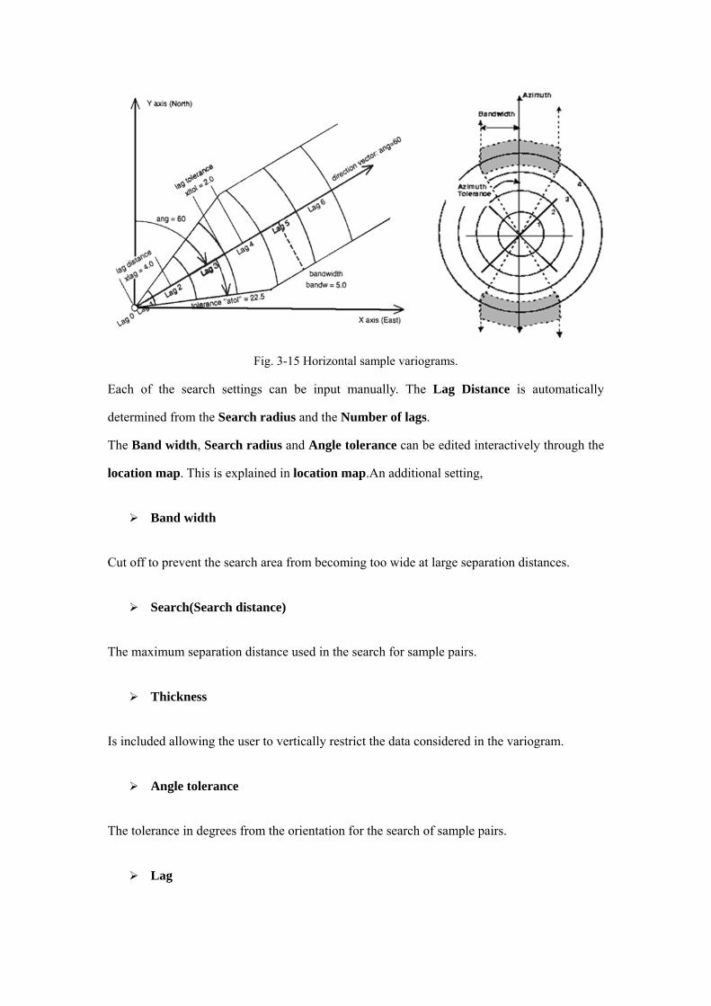
Fig. 3-15 Horizontal sample variograms.
Each of the search settings can be input manually. The Lag Distance is automatically
determined from the Search radius and the Number of lags.
The Band width, Search radius and Angle tolerance can be edited interactively through the
location map. This is explained in location map.An additional setting,
Band width
Cut off to prevent the search area from becoming too wide at large separation distances.
Search(Search distance)
The maximum separation distance used in the search for sample pairs.
Thickness
Is included allowing the user to vertically restrict the data considered in the variogram.
Angle tolerance
The tolerance in degrees from the orientation for the search of sample pairs.
Lag
Subdivisions of the range.
Lag tolerance
Distance from the lag at which data will be considered as belonging to that lag. This is quoted
as a percentage of the lag distance. For example, 50% means that all points will belong to one
lag, greater than 50% means that some same data may be considered in two lags, less than 50%
means that some data may not be considered.
⑨ToolButtons
Fit variogram to regression curve——Fit the Variogram model to the best fit.
Show No pairs histogram——Toggle the histogram on and off.
Refresh
⑩ Location map
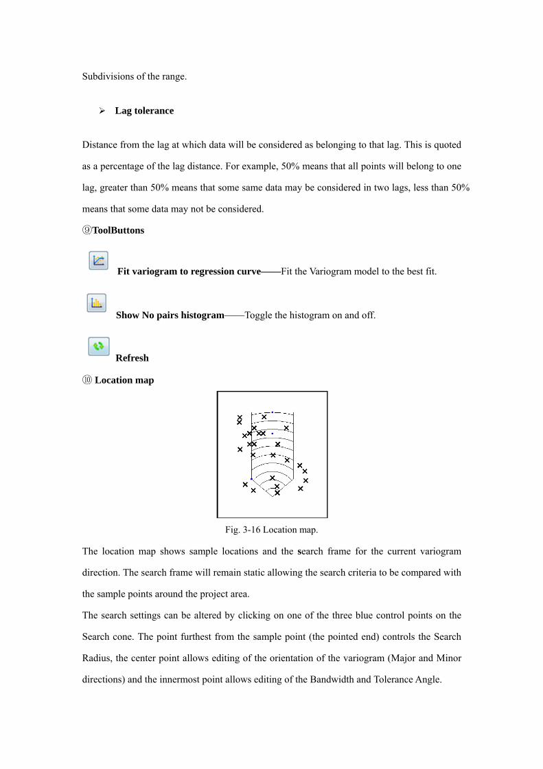
Fig. 3-16 Location map.
The location map shows sample locations and the search frame for the current variogram
direction. The search frame will remain static allowing the search criteria to be compared with
the sample points around the project area.
The search settings can be altered by clicking on one of the three blue control points on the
Search cone. The point furthest from the sample point (the pointed end) controls the Search
Radius, the center point allows editing of the orientation of the variogram (Major and Minor
directions) and the innermost point allows editing of the Bandwidth and Tolerance Angle.

⑪Variogram plot
Fig. 3-17 Variogram plot introduction.
It has three elements:
Histogram
This shows the number of sample pairs in each Lag.
Sample Variogram
These are the blue points showing the semi-variance in each Lag.
Variogram model
The current variogram model (black curve).
(3) Histogram window
Fig. 3-18 Histogram window introduction.
The histogram shows the distribution of the chosen property before or after the chosen
transformations have been performed.
①Intervals

——Defines the number of bins the data is divided into for the histogram display.
②Sample Num
——Number of data points.
③Min
——Minimum of data points.
④Max
——Maximum of data points.
⑤Mean
——Mean of data points.
⑥Std
——Standard deviation.
⑦%
——Toggle between percent and number of samples for the histogram
⑧Show
——Histogram choice between input, output and final.
⑨Refresh
——Apply the settings of the current transformation.
3.3 Simulation methods
Fig. 3-19 Available simulation methods.
3.3.1 Sequential Gaussian Simulation (SGS)
The Sequential Gaussian Simulation is a stochastic algorithms of interpolation based on
Kriging.

What is stochastic algorithms?
Stochastic algorithms use a random seed in addition to the input data, so while consecutive
runs will give similar results with the same input data, the details of the result will be different.
Stochastic algorithms such as Sequential Gaussian Simulation are more complex and
therefore take much longer to run, but they do honor more aspects of the input data,
specifically the variability of the input data. This means that local highs and lows will appear
in the results which are not steered by the input data and whose location is purely an artifact
of the random seed used. The result will have a distribution more typical of the real case,
although the specific variation is unlikely to match. This can be useful, particularly when
taking the model further to simulation as the variability of a property is likely to be just as
important as its average value. The disadvantage is that some important aspects of the model
can be random and it is important to perform a proper uncertainty analysis with several
realizations of the same property model with different random seeds.
Sequential Gaussian Simulation honors well data, input distributions, variograms, and
trends. The variogram and distribution are used to create local variations, even away from
input data. As a stochastic simulation, the result is dependant on the input of a random seed
number and multiple representations are recommended to gain an understanding of
uncertainty.
3.3.2 Sequential Indicator Simulation (SIS)
It is a stochastic modeling technique.
Sequential indicator simulation (SIS) is most appropriate to where either the shape of
particular facies bodies is uncertain or where you have a number of trends which control the
facies type, for example, when using a seismic attribute to control the probability of the
occurrence of certain facies.
3.3.3 Kriging
Kriging is a deterministic algorithms.
What is deterministic algorithms?
Deterministic algorithms will always give the same result with the same input data. These
algorithms will generally run much quicker and are very transparent - it is easy to see why a
particular cell has been given a particular value. The disadvantage is that models with little
input data will automatically be smooth even though evidence and experience may suggest
that this is not likely. Getting a good idea of the uncertainty of a model away from the input

data points is often difficult in such models.
Kriging is an estimation technique that use a variogram for expressing the spatial variability
of the input data. The user must specify the variogram model type, orientation, nugget and
range. The algorithm will not generate values larger or smaller than the min/max values of the
input data.
3.3.4 Indicator Kriging
Indicator kriging is a deterministic algorithms for kriging discrete properties.
Advantages
It is a deterministic (estimation) method, so the results are directly repeatable and it avoids
over interpretation of the data.