Henry Ford Hospital Medical Journal

Volume 24 | Number 3 Article 7

9-1976

Use of the Weibull distribution for analysis of aclinical therapeutic study in rheumatoid arthritisW. R. McCrum

J. T. Sharp

G. B. Bluhm

Follow this and additional works at: https://scholarlycommons.henryford.com/hfhmedjournalPart of the Life Sciences Commons, Medical Specialties Commons, and the Public Health

Commons

This Article is brought to you for free and open access by Henry Ford Health System Scholarly Commons. It has been accepted for inclusion in HenryFord Hospital Medical Journal by an authorized editor of Henry Ford Health System Scholarly Commons.

Recommended CitationMcCrum, W. R.; Sharp, J. T.; and Bluhm, G. B. (1976) "Use of the Weibull distribution for analysis of a clinical therapeutic study inrheumatoid arthritis," Henry Ford Hospital Medical Journal : Vol. 24 : No. 3 , 173-182.Available at: https://scholarlycommons.henryford.com/hfhmedjournal/vol24/iss3/7

Henry fbrd Hosp. Med. Journal

Vol. 24, No. 3, 1976

Use of the Weibull distribution for analysis of a clinical therapeutic study in rheumatoid arthritis

W. R. McCrum, PhD *, J. T. Sharp, MD * * , and G. B. Bluhm, MD

* Department of Neurosurgery and Neurology, Henry Ford Hospital

•'Department of Internal Medicine, Rheumatic Disease Section, Baylor College of Medicine, Houston, Texas, 77025

*** Division of Rheumatology, Henry Ford Hospital

Address reprint requests to Dr. McCrum at Henry Ford Hospital, 2799 West Grand Boulevard, De-troftMl 48202

This paper introduces the use of the Weibull distribution function for the analysis of small samples of clinical data. It is com­pared with the use ofthe conventional anal­ysis of variance in determining the results of a study comparing the use of gold salts and a placebo in the treatment of rheumatoid arthrids.

Although the samples were small, 14 con­trol patients and 13 who were treated, analy­sis of variance determined several significant differences between the two groups. The use of the Weibull distribution, however, not only confirmed these differences, but also determined several more differences be­tween the two groups that were undetected by analysis of variance.

A brief description and discussion of the Weibull distribution function is presented. It Includes a method for determining the Weibull parameters, and the use of these parameters in identifying unknown samples as belonging to more well-known distribu­tion functions such as the normal, exponen­tial and Chi Square.

A method for comparing two samples using an integration ofthe sum of the alpha and beta errors is also presented.

Finally there is offered an explanation as to why the use of the Weibull distribution should be more sensiUve in determining differences between small samples of data than more conventional methods of hypoth­esis testing.

173

Analysis of clinical data

I N 1951 Waloddi Weibull described a sim­ple distribution function with the only condi-t i ons tha t it be n o n - z e r o and n o n -decreasing.^ He said the function had wide applicability and presented seven examples ofthe useofthisfunction in statistics. Most of the examples were in biostatistics. In one example (the fatigue life of steel) the inde­pendent variable was time; subsequently this use of the function as a failure rate distribution has been found most useful in reliability testing. It isalso finding increasing acceptance in engineering and physics for use in other than life testing procedures. Johnson and Leone^ refer to "Weibul l iz ing" a variety of distribution functions such as the normal, exponential, beta, gamma and Chi Square. However, its use has been almost totally neglected in the field of biostatistics, as described in his remaining examples. The purpose of this paper is to show that this function is useful in evaluating clinical data and has theoretical advantages over the classical statistical hypothesis-testing tech­niques which assume a normal distribution. To illustrate these points the Weibull dis­tribution is compared with analysis of vari­ance in evaluating a double blind trial of gold therapy in rheumatoid arthritis.

Gold salts have been used to treat rheu­matoid arthritis for many years. However, there are few studies on the effectiveness of this treatment. Recently Sigler etaP reported that some features of the disease were im­proved by treatment with gold salts, using analysis of variance for data evaluation. It was recognized that the use of "classical" statistics such as analysis of variance or Student's " t " test was perhaps inappropriate for evaluating small samples of 13 and 14 data points. For this reason the data were re­evaluated using the Weibull distribution function. To our knowledge this is the first application forthe Weibull distribution func­tion to a therapeutic trial.

Methods

A. Clinical Twenty-seven patients meeting the ARA

criteria for classical rheumatoid arthritis, and with the disease of less than 5 years' dura­tion, were randomized to either a control or treated group. There were 14 patients in the control group and 13 in the treated group. The similarity of disease severity and dura­tion in the two groups was established pre­v iously . ' Gold salts or placebo were administered for at least two years. The patients were examined at specified times regularly throughout the study."* The details o f t h e c l in ica l measurements evaluated herein were published previously.'

This paper compares the initial pre-treat-ment examinations and the examinations at 6, 12 and 24 months. The differences be­tween pre-treatment and subsequent mea­surements of grip strength, ring size, joints showing synovitis, walking time and lace tying time were analyzed. The serum pro­teins were determined at the beginning and at the end of the study.

B. Stadstical Since our samples are drawn from un­

known populations, the population param­eters must be estimated from the samples. This is true of any statistical procedure when the population parameters are unknown. The Weibull distribution uses three param­eters to identify the population. These are the: origin (alpha), the shape (beta) and the scale (theta). Thus the cumulative Weibull distribution function:

F(x) = 1-

and the density function;

•1 f(X) = /3 (X -a ) • V e-a )

It is evident that F (x) is a log log function. When the relationship between the log-

174

McCrum, Sharp and Bluhm

arithmic values of the sample x and the log log values of F (x) is linear, the sample is said to have come from a population having a Weibull distribution. Thus the slope of the best fit line through the sampledata points is the best estimate of the shape parameter beta. The intercept of this line with the abscissa yields the origin (parameter alpha). When X = theta the Weibull function re­duces to

F(x) = 1 -e 0.632.

For this study a computer was used to deter­mine the best fit line through the data using successive estimates of alpha as a starting point. Appendix 1 describes the format ofthe computer program used in determining the parameters of samples of grip strength in the control and treated groups.

Having established the Weibull param­eters for our two samples to be compared, we then establish the probability of a dif­ference between them as a confidence " c " . This in essence represents the minimum integral or overlap of the Type 1 (alpha) and Type 11 (beta) errors of classical hypothesis testing. The use of alpha and beta in this instance should not be confused w i th Weibull parameters having the same name. The rationale for the confidence " c " is ex­plained by L. G. Johnson." Since that pub­l icat ion has a l imi ted c i rcu la t ion , the introduction to the article is reproduced in Appendix III.

Results

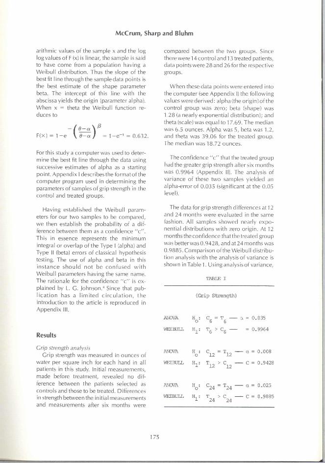
compared between the two groups. Since there were 14 control and 13 treated patients, data points were 28 and 26 forthe respective groups.

When these data points were entered into the computer (see Appendix 1) the following values were derived: alpha (the origin) of the control group was zero; beta (shape) was 1,28 (a nearly exponential distribution); and theta (scale) was equal to 17.69. The median was 6.5 ounces. Alpha was 5, beta was 1.2, and theta was 39.06 for the treated group. The median was 18.72 ounces.

The confidence " c " that the treated group had the greater grip strength after six months was 0.9964 (Appendix II). The analysis of variance of these two samples yielded an alpha-error of 0.035 (significant at the 0.05 level).

The data for grip strength differences at 12 and 24 months were evaluated in the same fashion. All samples showed nearly expo­nential distributions with zero origin. At 12 months the confidence that the treated group was better was 0.9428, and at 24 months was 0.9885. Comparison ofthe Weibull distribu­tion analysis with the analysis of variance is shown in Table 1. Using analysis of variance,

TABLE I

(Grip Stirength)

ANOVA

WEIBULL H,

^6 = ^6

6̂ > S

a = 0.035

= 0.9964

Cnp strength analysis Grip strength was measured in ounces of

water per square inch for each hand in all patients in this study. Initial measurements, made before treatment, revealed no dif­ference between the patients selected as controls and those to be treated. Differences in strength between the initial measurements and measurements after six months were

ANOVA H :

WEIBULL H,

ANOVA

WEIBtILL H,

= ^12

^24 " ^^24

T > C 24 24

a = 0.008

C = 0.9428

a = 0.025

C = 0.9885

175

McCrum, Sharp and Bluhm

the null hypothesis Ho is accepted if the a error is > 0.05. Using the confidence meth­od the Hypothesis H, is accepted if " c " is > 0.90. In this instance there was no conflict between analysis of variance and the confi­dence method. Ho was rejected by the for­mer and H| accepted by the latter.

The choice of a 0.90 confidence level is purely arbitrary in this instance. It is the usual level of confidence accepted in physics and reliability engineering, and was considered in this case an acceptable level for the purpose of the study. It must be remembered that we are considering the probability of a difference between two samples whereas in using analysis of variance the level of the alpha error is not necessarily indicative of a difference between two samples. In point of fact, selection of too small an alpha error (0.01 for instance) may mask the correct probability of a difference by creating too large a beta error. This point is enlarged upon later.

Ring size analysis

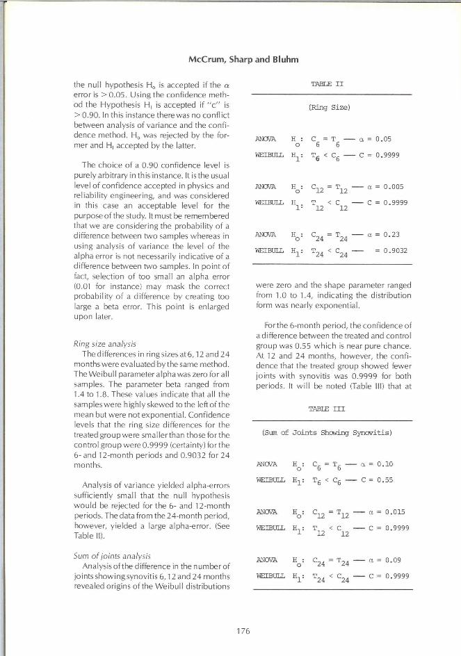
The differences in ringsizes at6,12 and 24 months were evaluated bythe same method. The Weibull parameter alpha was zero for all samples. The parameter beta ranged from 1.4 to 1.8. These values indicate that all the samples were highly skewed to the left ofthe mean but were not exponential. Confidence levels that the ring size differences for the treated group were smaller than those for the control group were 0.9999 (certainty) for the 6- and 12-month periods and 0.9032 for 24 months.

Analysis of variance yielded alpha-errors sufficiently small that the null hypothesis would be rejected for the 6- and 12-month periods. The data from the 24-month period, however, yielded a large alpha-error. (See Table II).

TABLE I I

CRing Size)

ANOVA H : C = T o 6 6

WEIBULL H, 6̂ < S

ANOVA H : C , = T

WEIBULL H

ANOVA H

12 "12

T < C 12 12

S 4 = ̂ 24

WEIBULL : T , . < C.,̂ 1 24 24

a = 0.05

C = 0.9999

— a = 0.005

— C = 0.9999

— a = 0.23

— = 0.9032

were zero and the shape parameter ranged from 1.0 to 1.4, indicating the distribution form was nearly exponential.

Forthe 6-month period, the confidence of a difference between the treated and control group was 0.55 which is near pure chance. At 12 and 24 months, however, the confi­dence that the treated group showed fewer joints with synovitis was 0.9999 for both periods. It wi l l be noted (Table 111) that at

TABLE I I I

(Sum of Joints Showing Synovitis)

ANOVA H : = T , o 6 6

WEIBULL H-^: Tg < Cg

ANOVA H : C,_ = T - . 0 12 12

WEIBULL H, : T < C 1 12 12

a = 0.10

C = 0.55

— a = 0.015

— C = 0.9999

Sum of joints analysis Analysis ofthe difference in the number of

joints showing synovitis 6,12 and 24 months revealed origins ofthe Weibull distributions

ANOVA H^: C^^ = T24

WEIBULL : T..,, < C 1 24 '24

a = 0.09

C = 0.9999

176

Analysis of clinical data

both the 6-month and 24-month evalua­tions, the alpha-error was essentially the same, whe reas the c o n f i d e n c e leve l changed from 0.55 to 0.9999. This points out the importance of considering the beta-error as well as the alpha-error in determin­ing differences between samples. This be­comes especially important when dealing with highly skewed distributions as in this case.

Walking dme analysis Initially the treated and control groups

showed no difference in thetime required to walk a measured distance. Differences in walkingtime were calculated at6,12 and 24 months. Both treated and control patients showed a decrease in walkingtime over the entire length of the study. At 6 months the decrease in time was similarfor both groups. At 12 and 24 months, however, the treated group showed a greater decrease than the control group with the high probability, " c " = 0.9999 for both 12 and 24 months, that these changes were valid. These samples were also nearly exponentially distributed. Analysis of variance failed to indicate any differences between the treated and con­trols, (see Table IV).

Serum proteins analysis Serum protein electrophoresis was per­

formed on samples from each subject at the beginning and end of the study. There were no differences between the treated and con­trol groups in either total protein, albumin or globulin at the beginning. At the end of the study there was no change in total protein but albumin values were lower (c = 0.956) and globulin levels higher (c = 0.981) in the control group than in the treated group. Analysis of variance showed only the al­bumin level to be lower in the control group at the end of the study (see Table V).

Tests showing the treatment effect Several other measurements were evalu­

ated which showed no differences between the treated and control groups by either the ANOVA or Weibull methods. These tests

TABI£ IV

CWalk±ng Time)

6 inontils

H : o

C T a = 0.75

T < C C = 0.58

12 mont±is

«o = C = T a = 0.75

H : 1

T < C C = 0.9999

24 ittoiths

H : o

C = T a = 0.75

T < C C = 0.9999

include lace tying time, hemoglobin, and white blood cell count.

Discussion

The Weibull distribution function is a very convenient and flexible probability distribu­tion. Itrequiresofthe sample data only that it be non-zero and non-decreasing in its cumulative sum. It is widely used in industry because empirically it has been proven relia­ble in evaluating small samples of test data. Almost all medical data sets fit these condi­tions. Yet use of the Weibull distribution for evaluatingclinical data has had such limited application that it is essentially a new ap­proach. Its use, therefore, deserves careful consideration.

Perhaps its strongest attribute for its useful­ness is its ability to replace a number of

177

McCrum, Sharp and Bluhm

TABLE V

(Serum Proteins)

To ta l Protein

H : = c — a = 0.35 o I I

^1 <

^ 1 C = 0.7332

H : o = a = 0.75

"1 = < Cp C = 0.8039

Albumin

H : o

C = 1

T I

a - 0.26

H : 1

C, < T I

C = 0.8044

Ho = CF = Tp a = 0.028

Cp < TF C = 0.9562

Globulin

H : o

Cl = T j a = 0.08

% = Cl < Tl C = 0.914

H : o S = TF a = 0.005

Cp < Tp C = 0.9811

essentially a normal distribution. A value lessthan 3.5 indicates skewingof the data to the left of the mean and a value greater than 3.5 shows skewing to the right of the mean.

If the parameters ofthe parent population are unknown, then for any statistical in­ference the sample must be assumed to be a random sampleofthat population. Since this must be the case, the parameters of the sample are the best estimators ofthe param­eters of the parent population. Thus, for example, if the sample is exponentially dis­tributed, it must be assumed that the parent population is also exponentially distributed. In such case the parameters of mean and variance wi l l have little or no usefulness in establishing a meaningful inference. On the other hand, if it is arbitrarily assumed that the parent population is normally distributed then it is obvious that the exponentially distributed sample is nota random sample of that population. A statistical inference in such case would not be valid. If the Weibull parameters of the sample are established first, errors concerning population character wi l l not be made. This is in contrast to using analysis of variance. In using analysis of variance, as in the present study, the mean and variance of the population were esti­mated from the sample. This required two arbitrary assumptions: 1)the parent popula­tion was normally distributed, and 2) the sample was a truly random representation of this normal population as defined mathe­matically (5) by the relationship:

better-known functions such as the normal, exponential, Chi Square, gamma and beta distributions. When the shape parameter beta equals one the distribution becomes exponential.

F(x) 1 -e

Further, it has been determined empirically that when the shape parameter equals 3.5 the mean and median coincide and we have

P{XK • Xk — Fk ( x „

In point of fact, neither of these assumptions was supported by the data available from this study. As can be seen from the results most of the samples were either exponen­tially distributed or highly skewed to the left of the mean. It may be argued that small samplesdrawn from normal populations are skewed and corrections can be made forthe skewness. This argument is valid only when the population distribution is known with certainty.

178

Analysis of clinical data

The distribution functions of biological data are generally not known, and, further­more, should not be assumed to have a normal distribution. This is particularly true if the data are oriented in the time domain. Clinical studies often are concerned with a " l i fe " process, either that of the patient or of a disease. Such " l i f e " processes differ in their distribution functions. Some are char­acterized by "infant mortality", some by "random decay" and others by "old age survival". This being the case, such studies should be evaluated by an appropriate " l i fe testing" distribution such as the exponential, log normal, gamma, etc. The Weibull dis­tribution proves most useful in this regard because it characterizes most of these. As mentioned before, Weibull parameters ade­quately describe numerous d is t r ibut ion funct ions inc lud ing the normal and Chi Square.

Another advantage ofthe Weibull method is that populations can be compared at different percentiles other than the mean. Thus two different groups can be compared at10% level, 90% level orthe 50% level (the median). Analysis of variance and Student's " t " test compare only the means, which usually vary from the 40th percentile to the 60th percentile, depending on the amount and direction ofthe skewness ofthe popula­tion. Thus, for example, some treatment might make 10% of the population worse, improve another 10%, but "on the average" show no effect. This could be revealed by Weibull analysis at varying percentiles.

The shape parameter beta may also be compared fordifferent Weibull distributions. It may happen that two populations wi l l "average out" equally but the character of their distributions may be quite different. These differences can be determined and q u a n t i f i e d by e v a l u a t i n g the shape parameter.

In the study reported here, most of the conclusions based on evaluation by the Weibull analysis were in agreement with

those reached by analysis of variance. In some instances, however, analysis of vari­ance failed to detect small differences be­tween the treated and control groups that were held to be significantly different when evaluated by the Weibull method. The basis for such discrepancies has already been discussed. In the present study in particular two factors stand out.

In the first instance analysis of variance depends upon the mean and variance for information. Since most data samples in this study were nearly exponential in distribu­tion, their mean and variance carried little meaningful information.

In the second instance the consideration of only alph-errors ratherthan consideration of both alpha and beta errors together is emphasized. In classical statistics, an in­ference is accomplished by hypothesis test­ing. An hypothesis is made, and from the sample data a probability of an error is established if the hypothesis is accepted. This probability is called the alpha-error. A probability that an error wi l l be made if the hypothesis is rejected is also present. This probability is Called the beta-error. The two probabilities are mutually exclusive; both the alpha-error and the beta-error contribute to the total probability of an error in either accepting or rejecting the hypothesis. The correct level of probability that should be chosen for rejecting or accepting an hypoth­esis then is that level which minimizes the sum of the alpha and beta errors (see Appen­dix 111). In actual practice this is rarely done. An alpha-error (usually very small) is ar­bitrarily chosen, and the hypothesis is ac­cepted or rejected, depending on the alpha-error calculated from the samples.

The We ibu l l analysis uses a di f ferent method of making a statistical inference. A "confidence" is established which is a mea­sure of the overlap between two adjacent probability density functions. It is then in essence an integration of the alpha and beta errors, (Figure 1).

179

McCrum, Sharp and Bluhm

CONTROL

\

TREATED /

DISTRIBUTION OF MEANS

. Computed \ alpha error

r

/ IMTK. \ beta 11 error^fl

1^^= II lllillilNIIINHTTr*̂ 1 \ 0 1=0.23 /

ANOVA method accepts the NULL HYPOTHESIS

WEIBULL method rejects the

NULL HYPOTHESIS

Figure 1 Hypothesis testing of ring size difference at 24 months. Comparison of hypothesis testing using a predetermined alpha error, as in ANOVA, with the confidence level determined by integrating the overlap

of the alpha and beta errors.

Conclusion

We believe that the application of Weibull distribution analysis to clinical data, as illus­trated in the gold trial reported here, is valid and wil l yield reliable results. In addition.

the method appears to be sensitive in detect­ing small differences in small samples. A major advantage in using the Weibull dis­tribution for clinical data analysis is that one does not have to assume the population has a particular shape such as bell-shaped curve

180

Analysis of clinical data

of the norma l d is t r ibut ion or the decay ing

s lope o f an exponen t ia l d is t r ibu t ion . The

shape is de te rmined f rom the sample, m u c h

as the shape o f t h e Chi Square d is t r ibu t ion is

de te rmined by the sample. W e bel ieve that

W e i b u l l d is t r ibut ion analysis deserves w i d e r

tr ia l in c l i n i ca l p rob lems since on ly exper i ­

ence f rom more extensive use w i l l establish

its true va lue.

A c k n o w led g e m e n t s

T h e a u t h o r s w i s h to t h a n k the J. M .

Richards' Laboratory, Grosse Pointe Park,

M i c h i g a n , for its con t r i bu t i on o f compu te r

t ime and programs in c o m p l e t i n g this pro­

jec t ; and the M i ch igan Chapter, Ar thr i t is

Foundat ion, for the grant to suppor t the

c l i n i ca l study.

References

1. Weibull W: A statistical distribution function of wide applicability./ Appl Mechanics 293-297, Sept 1951

2. Johnson NL and Leone FC: StaUstics and Ex­pe r imen ta l Design in Engineer ing and the Physical Sciences. Vol I, John Wiley and Sons, New York, pp 112-115, 1964

3. Sigler JW, Bluhm GB, Duncan H, Sharp |X Ensign DC, and McCrum WR: Gold salts in

treatment of rheumatoid arthritis. Ann Intern Med 80:21-26, 1974

4. Johnson LG: Sample comparison vs hypothesis testing. Stadstical Bulledn of the Detroit Re­search Institute 2:104, 1972

5. Fisz M: Probability Theory and Mathemaucal StatisUcs, 3rd Ed, John Wiley and Sons, New York, 335-336, 1963

APPENDIX I

Computer Program Format for Weibull Parameters of Grip Strength of Treated Patients

Input

Step 1. Step 2.

Output

Step 1.

Step 2. Step 3. Step 4. Steps. Step 6.

Estimates of origin (alpha): 0, 5, 10. Data (not ordered): x,, x^, X24.

Data (ordered listing): Xj,, Xj2, . . . . Xj24.

Median ranks of: Xj,, Xj2, Xj24. Origin (alpha) = 0 (from input). Shape (beta) = 1.0280. Scale (theta) = 43.6483. Goodness of fit = 0.9500.

Step 7. Median = 18.8633. Step 8. Origin (alpha) = 5 (from inpuO.

Step 9. Shape (beta) = 1.1231. Step 10. Scale (theta) = 39.0681. Step 11. Goodness of fit = 0.9705. Step 12. Median = 18.72. Step 13. Origin (alpha) = 10 (from input). Step 14. Shape (beta) = 10.0581. Step 15. Scale (theta) = 29.2672. Step 16. Goodness of fit = 0.9371. Step 17. Median = 18.8111.

Comment

The best goodness of fit test equals 0.9705 (Step 11). Therefore the best estimates of the Weibull parameters are: alpha = 5 (Step 8), beta = 1.1231 (Step 9) and theta = 39.0618 (Step 10).

1= Distribution of PARAMETER |

OVERLAP AREA

OR INTERFERENCE

AREA

Distribution of PARAIVIETER2

X=Value of Parameter-^

181

McCrum, Sharp and Bluhm

APPENDIX II

Computer Program Format for "Confidence" of a Difference in Grip Strength Between Treated

and Control Groups.

Input

Step 1.

Step 2.

Step 3. Step 4.

Output

Step 1.

Step 2.

Step 3.

Step 4.

Step 5.

Comment

Control group values: alpha = 0, beta = 1.276, theta = 17.69, sample size = 28.

Treated group values: alpha = 5, beta = 1.1231, theta = 39.06, sample size = 24. Percentile compared = 0.5 (median). Null ratio = 1 (at least different).

Estimated mean of control population = 14.329. Estimated standard deviation of control population = 2.836. Estimated mean of treated population = 31.97. Estimated standard deviation of treated population = 6.43. Confidence = 0.9964.

Given the Weibull parameters for two samples, the program compares the two samples at any percentile level and at any selected magnitude of difference. In this example the medians were compared and found to be at least different with a confidence 0.9964. If we had selected a null ratio of 2, then the program would have computed the confidence that the median of one sample was at least twice as large as the median of the other sample.

APPENDIX III

From Statistical Bulletin: Reliability & Variation Research. Leonard G. Johnson, Editor, Vol. 2,

Bulletin 2, May 1972, Page 1.

Sample comparison vs hypothesis testing

In comparing two samples we calculate the confidence C that one ofthe samples represents a population which is superior to the population represented by the other sample.

In testing the hypothesis that a given sample belongs to a population superiorto some standard population we specify so-called a and /3 errors, and determine whether under the {a, /3) pair chosen we should acceptor reject the hypothesis t ha t the s a m p l e b e l o n g s to the s t a n d a r d population.

The question which now can be asked is " H o w are these two statistical techniques related (i.e., sample comparison and hypothesis testing)?" More specifically, we can ask "What is the rela­tionship between a, j i , and C?"

Acomparison of two samples is generally done by comparing a particular type of population parameter or quantile level in the two samples. The parameter chosen could be the mean in the case of normal distribution, or characteristic val­ues n the case of Weibull distributions.

The corresponding hypothesis which istested is then the one which states that the mean of an observed sample belongs in population^ with meani, or that the characteristic value 9 of an observed sample belongs in population^ with characteristic valuex = Si (̂ ^ and being the characteristic values of the two possible popula­tions from which the sample could come).

In order to make a comparison of parameters vs parameteri we need distribution functions for both parameters {say, the estimated mean of popula­tions) and parameters (the estimated mean of popu/a!/on2).

Once these distribution functions are known we construct an interference diagram, as in Figure 1.

Bulletin No. 2, Page 2

From Figure I it is possible to calculate the probability that a random element from II exceeds a random element from I. Thisisthen definedtobe the confidence that parameters > parameters.

Let the PDF (Probability Density Function) of I

be fl (X).

Let f l (X) = PDF of II.

Let Fl (X) = CDF (Cumulative Distribution Function) of I.

Let F2 (X) = CDF of II.

Then

C = j V i (X) f2 (X) dX

According to formula 1 the confidence C in­creases as in the overlap area between fi (X) and f2 (X) is made smaller, until when there is no overlap, the confidence becomes 1 (i.e., 100% or certainty) that whatever is selected in II wi l l surely exceed whatever is selected in I. On the other hand, i f f i (X) and f2 (X) are identical (100% overlap), it follows that there is a 50-50 chance (i.e., 50% confidence orC-.5) thatthe selection from II wi l l exceed the selection from I.

182