RADIO SCIENCE Journal of Research NBS/USNC- URSI Vol. 690, No.4, April 1965

Use of the Phase-Integral Method to Determine the Reflection Properties of a Stro tified Ionosphere

C.Altman 1

Official Communication From D.S.I.R. Radio Research Station, Slough, Bucks, England

(Received October 15. 1964; revised November 23. 1964)

A Pegas us computer has been programmed to give the absorption coefficients and virtual heights a t ve rtical incide nce for the main magneto-ionic compone nts re fl ected from a s tratified ionosphere. using the phase integral method. Typical absorpt ion and virtual height curves are given for daytime ionospheri c models. For high geomagnetic latitudes the Z-trace is shown to be one of the two least a ttenuated traces for daytime E-layer reflections at freque ncies both above and below the gyrofre· quency. and it is shown that under certain c ircums tances the Z-trace may appear at a lower virtual height than the O-trace. The limitations of the usual ray me thod which uses the group refractive index for de termining virtual height s are discussed. and it is s hown that a s imple correction te rm may be added to the ray theory calcul a ti on of virtual heights to make it agree with the phase integral de termina tion .

1. Introduction

The reflecting properties of the ionosph ere have been calculated numerically by two main techniques. The most accurate is probably the 'full-wave' method in which the first order equations derived from Max­well's equations and the ionospheric co nstitutive relations are solved by a step-by-step integration . The method, described by Budden [1955], Barron and Budde n [1959] and others, obtains the solutions in terms of the electri c and magne tic wavefi elds in per­pendicular directions. A recent variant of thi s tech­nique given by Pitteway [1964] considerably simplifi es the integration procedure by obtaining solutions in terms of two independe nt solutions of the wave equa­tion which are not coupled and which in many impor­tant cases are similar to the charac teri s tic magneto­ionic modes. The full-wave me thod is suited particularly to low-frequency analysis, whereas at higher fr eque ncies the large number of steps required makes the integration prohibitively long. The results obtained by the full wave technique are not readily applicable to the propagation of pulses, especially to the calculation of virtual heights, since the perpen­dicular components in the Budden method, or the non­coupled modes in the Pitteway method, must first be 'unravelled' and reconstituted into characteristic magneto-ionic modes in order to permit the differen­tiation of phase with respect to frequency which yields the virtual heights of the 0- and X-traces. The diffi­culty is enhanced whe n two modes having the same polarization, e .g., the 0 and Z modes, exist simultaneously.

The second important technique, the phase integral method, has been described by Budde n [1961], Cooper [1961], and others. It involves integrating the complex refractive index n, from ground level

IOn leave of absence fro m the Technion , Is rael Ins titute of Technology, Haifa. Israe l.

usually, up to the " height" (usually a complex quan­tity) where n becomes zero; i.e., up to one of the reflection branc h points of the complex refractive index. There will generally be two or three suc h reflec tion points , depe nding on whe ther the frequency is below or above the gyrofrequency. In addition there will be a coupling branch point at a complex height where the refractive indices for the character­istic magne to-ionic mod es become equal. A contour of integration whic h encompasses the coupling point (in the sense that the coupling point lies between the contour and the real axi s) will represent a coupling transition from one characteris tic mode of polariza­tion to another. No t all paths of integration connec t­ing the reflection points to ground are physically significant [Budden, 1961]. In general there will be four di s tinct contours of integration associated with modes of refl ec tion which will give independent traces on an ionogram - provided the absorption losses are not too high. The virtual height of reflection is deduced by evaluating the real part of Jndz over these integration paths for two adjacent freque ncies, and the imaginary part of Jndz gives the overall absorption. The solutions thus give the type of information which is directly comparable with the results of pulse re­flection experiments and may be used to compare the properties of theoretical models of the ionosphere with those actually observed.

2. Theoretical Considerations

2.1. Appleton-Hartree Formula and the Branch Points

The complex refractive index n is given by the Appleton-Hartree formula, which is used in the form

n 2 = 1- X(l-X-iZ) . 2(} (2.1)

(l -iZ) (l-X -iZ) - f2 sJn2 ± VF

511

where

F y4 sin4 () +}'2 cos2 () (1 _ X - iZ) 2 4 . (2.2)

The symbols are the usual magneto·ionic parameters

Ne2 • • l' d ' d (2 f) 2ID ratlOnalZe UnIts , e an

Eom 7T X

m being the electronic charge and mass respectively, I the wave frequency, Eo the electric permittivity of

free space, and N the number of electrons per unit volume.

Y =lfI = JeJB where Ifl is the gyrofrequency and B I m is the induction of the earth's magnetic field.

Z =~ where v is the electronic collision frequency . 27TI

() is the inclination of the earth's magnetic field to the vertical.

In formula (2.1) the square root of the complex quan· tity F is chosen using the co mputer' s complex square root subroutine, so that the real part is always posi­tive . When the plus sign is used, the wave will be called ordinary, and the minus sign will correspond to the extraordinary wave. The quantity F, (2.2) may be rewritte n in the form

F = }'2 cos2 () [(Z~ _Z2) + (X -1)2 +2iZ(X-I)] (2.3)

where Z c y sin2 () 2 cos ()

Considering an upgoing wave in the ionosphere, initially it will be at a level where X < 1, so that the quantity F, (2.3), will have a negative imaginary com­ponent and will be in the third or fourth quadrant ?f the complex plane. At X = 1, F crosses the real aXIS and has the sign of (Z~ - Z2) . Thus if Z c > Z at X = 1 then VF changes continuously through X = 1, and so too does the complex refractive index n; but if Zc < Z at X = 1 then VF jumps discontinuously from the negative imaginary to posi tive imaginary. axis and c?n­tinuity of the refractive index n reqUlres reversmg the upper and lower signs as we cross the X = 1 level. Thus an 'initial ordinary' becomes extraordinary, and vice versa.

The complex refractive index n becomes zero when

X=I-iZ (2.4)

for the ordinary wave and

X=I±Y-iZ (2 .5)

for the extraordinary wave. These reflection points, labelled RO, RX +, and RX - respectively occur at com­plex heights which are usually well within a wave­length of the real axis.

The ordinary and extraordinary refractive indices (and polarizations) become equal at the coupling point

C, at a complex height where 2

X=I+i(Zc- Z ). (2.6)

The four points RO, RX +, RX -, and C are, in general, the four branch points of the complex refractive index surface.

In order to locate the bran ch points in the complex plane , it is necessary that X and Z be known analytic functions of z = x + iy, the complex he ight. If an arbitrary ionospheric model or ' profile' is used, e.g., if X a nd Z are experimentally derived functions of the height z, then in order to locate the branch points in the complex plane it is necessary in each case to approximate the X and Z variations at real heights in the neighborhood of these points by analytic functions, and then by substitution to solve (2.4) to (2.6) for com­plex z. In general the branch point closes t to the real axis is the one chosen.

2.2. Location of the Branch Points for Exponential Variation of X and Z

In the present investigation it has been assumed that log X and log Z vary linearly in the neighborhood of the branc h points, so that

X =Xo eaz

Z = Zo e- bz

(2.7)

(2.8)

where Xo and Zo are the values at X = 1 or X = 1 ± Y, and the constants a and b are determined by meas uring the slopes of the log X and log Z profiles, or of the chords across one or several tabular intervals near these points.

Substituting (2.7) and (2.8) into (2.4) and (2 .5) it is found that the coordinates (XR, YR) of the reflection points , measured from the X = 1 or X = 1 ± Y levels, are given by

11 [ cos bYR ] XR- - og - a cos (a + b)YR

=.!. log [Zo cos(~+ b)YR] . (2.9) b -Xo sm aYR

Here YR is necessarily negative and only such values of YR are accepted for which the arguments of the sin and cos terms are less than 7T/2. Inspection of (2.9) shows that if a a nd b are positive, i.e., if the X profile increases and the Z profile decreases with height, then XR > 0, i. e., the reflection points will lie at slightly greater heights than the X = 1 or X = 1 ± Y levels. For a positive and b negative as in the F region where electron-ion collisions predominate and consequently Z increases with height, x will often be negative .

2 A second coupling point at

X = l - iZc - iZ

whic h would be located far the r away from the real ax is, and would hence be less significant phys ically , has bee n ignored .

512

Substitution of (2.7) and (2 .8) into (2.6) yields the coordinates (xc, Yc) of the coupling point, measured from the X = 1 level, as given by

Xc =! log [cos byc - Z c sin bYe ] a cos (a + b)yc

=! log[ Zo cos(a+ ~)ye ]. b Z e cos aYe - sm ayc

(2.10)

Whe n Zc > Z at X = 1, the case of most general interes t at high frequencies, the positive value of Yc is chosen, and for Z c < Z at X = 1, the negative value of Ye· In general Xc may be pos itive or negative and Xc may be greater or less than XRO, i. e., the coupling point C may be either above or below the ordinary wave re­flection point RO.

Equations (2.9) and (2. 10) may be solved numerically on a computer. Equating the express ions involving y only, allows y to be found by means of a s uitable zero searc h proced ure, and X is the n give n explicitl y as a function of y.

2.3. Phase Integral Calculation of Absorption and Virtual Height

Having located the main branc h points , zo, the com­plex refrac tive index must now be integrated from the starting level, us ually the ground , along suitable con­tours up to these points and bac k again. The complex refl ection coeffi cie nt , measured at the ground , is give n by

exp [2;il (et - 2 (0 ndz)]

and the total absorption A suffered by the wave is (in nepers)

(2 .11)

Representing a pulse or wave packe t at the ground, by an ex pression of the type

f [47Ti (let [ZO ) ] B(f) exp ~ 2:-1 }0 ndz dl

we see that the phase at the ground will be stationary with respec t to I at a time t = T given by

(2.12)

yielding the virtual height of refl ection, hi. When X and Z are known analytic functions of z

it is frequently convenient to choose as contours of integration s traight lines in the complex plane joining the origin to Zo [Cooper, 1961]. But when X and Z are arbitrary tabulated functions of z it is necessary to perform the integration mainly along the real axis.

A convenient path is along the real axis to Xo =M (zo) and then parallel to the imaginary axis to Zo = Xo + iyo, X and Z having the assumed variation in this region given by (2.7) and (2.8). This particular choice of contours has the advantage of allowing a direct com­parison with simple ray theory.

Broadly s peaking, the real axis integration (excluding possibly the last wavele ngth of contour path in the reflection region) represents the W.K.B. solution of the propagation equations. The 'co mplex plane integra­tion' from the real axis down to the branc h point Zo, together with perhaps the las t wavelength of contour path on the real axis, serves as a 'connec tion formula' linking the ' upgoi ng' to the 'downgoing' W.K.B. solutions on the real axis. This co nnec tion formula represents the asymptotic approximation to the Airy integral solution of the propagation equations near the branch point where the W.K.B. solutions break down [Budde n, 1961]. The 'co mplex plane integration' is thus a mathe matical procedure for calculating the absorption loss and phase change spec ific to the re­flection (or coupling) process where the W.K.B. approximations are invalid .

The four main integration paths are shown sche­matically in fi gure 1. There are two paths correspond­ing to th e extraordinary waves (X waves) reflected at RX + and RX -, respectively, whic h are important above and below the gyrofrequency, respec tive ly. The ordin ary wave (0 wave) is reflected at RO, and the path yielding the Z-trace is tha t which proceeds from ground to the coupling point C in the ordinary mode and thence to RX + as ex traordinary. We s hall call the wave travelin g along this pa th the Z-wave .

Writing the complex refractive index

n= /1- - iX (2.13)

where /1- a nd X are the refrac tive and absorption indices respectively, and substituting Zo = Xo + iyo in (2.11), we obtain

y (X= l+lZc -lZl

C

t f--------' I ~ - -- ~-- - _I __ ~ __ ...,

(2.14)

t--.;.---, I o~--~~I~----4-----------1~---x

r t 1 1

RX­(X=I -Y-lZl

RO (X = 1- lZl

RX+ (X =1+Y-lZl

F IGURE 1. Schematic representation of the four main integratIOn paths.

Key: ordin ary waves; ------ - extraordinary waves.

513

Yo is of course negative and the real axis and complex plane absorptions are additive . The Z wave absorp­tion may similarly be split into real axis and complex plane contributions.

The virtual height calculation (2.12) is performed by calculating

[ r Zo ] [r Xo r x.,+iyo ] .:n I Jo ndz =1 Jo f-tdx + J x o Xdy (2.15)

for two nearly equal frequencies, thus gIVIng the derivative.

3. Results for Daytime Models

3.1. Ionospheric Models Used

U1 20 a: w "-w 3; 15 «

z Q 10 .... "-a: o U1

'" «

\ I \x- I \, X

\ /\ " I \ ........- \

FREQUENCY, f (Me/5)

,

3.5

FIGURE 3. Absorption curves for the Oslo model.

In order to demonstrate typical results of the com- The X + trace l/ < f ,,) is off scale .

puter programme two daytime ionospheric models have been chosen. In figure 2, curve A shows the electron density distribution in the D and E layers over Oslo at noon during a sunspot maximum equinox. This curve has been proposed by Piggott and Thrane [1964]. Curve B shows the variation over Slough at noon during a sunspot minimum equinox. The D-Iayer curve has been determined by Deeks [1964] and the E-Iayer 'nose' has been tentatively fitted to it by Piggott [1964, private communication]. The inclination of the earth's field to the vertical at Oslo and Slough are e = 17° and e = 22°, respectively, and the gyrofrequencies are If! = 1.3 Mc/s and If! = 1.28 Mc/s, respectively. The dashed curve represents the mean collision frequency adopted. The two electron density distributions contrast cases with relatively dense and relatively weak D-region electron densities, but also differ significantly in that the slopes, dN/dh, are quite different for most of the reflection levels at

125

E 120 ~ -.c

_ 115 .... I '::' w 110 I

..J « => 105 .... a: >

100

0.8 3.5

lhe frequencies used in our computations. FREQUENCY, f (Me/5)

120

E -'" 100

.... I <0 W 80 I

60

log10 v -5

FIGURE 2. The assumed variation of electron density, N, with height at equinox noon.

C urve A is for Oslo a l sunspot maximum and Cu rve B is for Slough, sunspot minimum. Curve C is the assumed height variation of elec tron coUision frequency II.

514

FIGURE 4. Virtual height curves for the Oslo model.

Vi a: w "-w 5 « Z 0

>= "-a: 0 U1

'" «

20

15

10

I I

I /x+ / I

I I

\ \ IX-I I /

\/ /\

/ " /' "'

/"' "' - .... -FREQUENCY, f (Me/5)

FIGURE 5. Absorption c~rves for the Slough model.

115 , E 110

, ' X+

-J:: ,

_ 115 I >- I I

'" I ~ 110 I

I ...J I ~ 105 / >- / a: / :; 100

0.8 1.0 1.5 1.0

FREQUENCY, f (Mc/S)

FIGURE 6. Virtual height curves for the Slough model.

3.2. Variation With Frequency of Absorption and Virtual Heights

Figures 3 and 4 show the absorption and virtual height variation for the Oslo model, and figures 5 and 6 repeat these for the Slough model. For all values plotted , Z < Zc at X = 1. Below the gyrofrequency the Q- and Z·traces are the least attenuated, and in the case of the Oslo model the X + absorption does not appear as it is off scale for freque ncies above 0.9 Mc/s. For both models used, an ionogram might be expec ted to show only an Q·trace toge th er with a muc h fainter Z·trace below about 2 Mc/s, while an X·trace would only appear near the penetration frequency of the Q·trace.

3.3. Complex Plane Contribution to the Total Reflection Loss

The complex plane contribution to the total absorp· tion (given by the second term in (2.14)) has been cal· culated for all branch points. It never exceeds 0.05 N p for the X = 1 + Y reflection in the Slough model and 0.015 Np in the Oslo model, and is quite negligible compared with the large real height absorp· tion in thi s mode. For Oslo the X = 1- Y absorption in the complex plane (expressed in nepers) is less than 1 percent of the total for all freq uencies above 2 Mc/s , and for Slough it constitutes some 5 percent (0.56 Np) at 2 Mc/s falling off to about 3 percent (0.18 Np) at 3 Mc/s. The Q·mode complex plane absorption near X=l is more significant. For Slough it constitutes 0.48 Np out of a total of 3.37 Np at 0.8 Mc/s, falling off to 0.24 Np out of 4.31 at 2.8 Mc/s. The Oslo figures are 2.67 out of 14.56 Np at 1 Mc/s falling to 0.26 out of 3.70 Np at 2.7 Mc/s. The main conclusion is that the complex plane absorption is generally significant only for the Q·wave and especially at the lower frequencies whic h are reflected in regions of higher collision frequen cy.

3.4. Virtual Height of the Z-Trace

An interesting feature of the Oslo virtual height curves is the appearance of the Z·trace below the

Q·trace at the low-frequency end. This is at first sight surprising when analyzed in terms of simple ray theory, which considers the Z·mode wave packe t to travel up to the coupling level near X = 1 in the Q·mode and then to travel in the X-mode to the 1 + Y refl ec tion level. The firs t part of the journey might be expec ted to contribute a virtual height equal to that of the Q·trace, and the second part to add an additional virtual height equal to the real height difference between the X = 1 and X = 1 + Y levels plus any retardation in this section. The explanation of this anomalous result in the light of the phase integral analysis is given in section 4.

3.5. The Z-Trace Intensity as a Function of Magnetic Latitude

The effect of increasing the angle of inclination 8 between the earth 's magnetic field and the vertical is to decrease sharply the amplitude of the Z·trace by increasing the coupling loss or, in terms of the phase integral, by increasing the complex plane contribution to the absorption integral, (2. 11). We find, for in· s tance, by using the Slough model di s tribution for a frequency of 1.1 Mc/s, and le tting the inclination 8 take successive values , 11.50 , 17°, 22°, 300 , and 45°, that the complex plane contributes an absorption loss (for two traversals, upgoing and downgoing) of 0.04, 1.2, 3.0, 7.1, and 19.2 Np respec tively. At 1.5 Mc/s the corresponding fi gures are 0.10, 2.5, 5.5, 12.9, and 30.0 Np respectively.

3.6. Accuracy of the Computations

The Q-mode absorption calc ulations for the above and other ionospheric models have been c hecked against calculations made by a phase integral pro­gramme developed by K. G. Budden for the Cambridge Edsac II computer. Agreement is good in all cases . Slight di screpanc ies can be traced to the different analytic approximation made to the electron dis tri· bution near branch points . In our programme the curves are assumed to be exponential over short distances; in the Edsac II programme various other methods of curve fitting were used. This has an effect both on the computed location of branch points, and also on the interpolated values of X and Z between relatively widely spaced tabular intervals. The Edsac II programme checks against Budden's and against Pitteway's full wave computations.

Virtual heights for the above and other models for the ordinary and extraordinary modes have been com­pared with results given by a Mercury computer programme developed by E. B. Thran e in Oslo. Agreement is again good in all cases.

4. Calculation of Virtual Heights by Simple Ray Theory and by the Phase-Integral Method

4 .1. Phase-Integral Correction to Ray Theory

In sec tion 2 it was s hown (2.12) that the virtual height

515

L

of reflection is given by the expression

d [( ZoJ) ] h' = dl'Yt I Jo n (z) dz . (4.1)

Since the upper limit of integration Zo is a function of I this may be written

(4.2)

where

n'= ~(fn) (4.3)

defining the complex group refractive index. Since Zo represents a reflection branch point, n(zo)

= 0, and hence we obtain

( Zo

h' = 'Yt Jo n'dz. (4.4)

Equations (4.1) and (4.4) are two equivalent phase integral expressions for the virtual height, but the method of evaluation will be different for each. Consider (4.4) first. Since n and hence n' are known analytic functions of frequency, n' may be calculated for all points on the integration path and then inte· grated to zoo This method is adopted by Cooper [1961]. If we compare this method with the ray theory formulation

Ix o h'= 0 p.,'dx (4.5)

(where p.,' =~(n') is the group refractive index) and ignore for a moment the fact that Xo in (4.5) is not quite equal to .'Yt (zo) of (4.4), we find one form of the phase integral correction t:.h', to the ray theory esti· mate. If OAIRI (fig. 7) is the integration path chosen, then

t:.h' = 'Yt ( n'dz= fYO X'dy (4.6) JAIR I A,R, 0

where X' is the group absorption index. The evalua· tion of this correction term necessitates doing a com· plex plane integration and is not readily evaluated if a phase integral computer programme is not avail· able.

The alternative method of evaluating h' as adopted in the present investigation is based on (4.1) and gives a clearer insight into the cause of retardation, yielding also a more useful expression for the correction 10 ray theory. The quantity

'YtvJozo(j) n(z)dz]

y

xO(fI) xO(f2) AI A2

-----~---~-~. x O~----------------T----r--------~

FIGURE 7. Contours in virtual height calculation.

OA1R 1 represent s an integration path 10 reflection point R, for a frequency /1 and OA2R'l is the same for a slightly higher freque ncy /'lo

is evaluated for two neighboring frequencies, It and /2, the integration paths being represented scnemat· ically by OAIR I and OA zR2, respectively (fig. 7). As II ~ /2 the virtual height is given by

or

h' = [f XO(fI\f2p.,(f2) - 11p.,(fI)}dx+ h Jxolf2) p.,(h)dx o x.(f,)

+ {fz J x(f2)dy A2R2

-II f x(fl)dy }] ((f2-/d (4.7) AIRI

Now the last bracketed term in the numerator repre­senting the difference between the complex plane integrations at neighboring frequencies is usually negligible compared with the first two terms. For instance for the Slough model in the entire frequency range considered, this contribution never exceeds 0.2 km for the 0, X, or Z waves (unless the absorption IS III excess of 100 Np). Hence (4.7) in the limit reo duces to

JX o dxo h'= p.,'dx+lp.,-·

o dl (4.8)

This equation may have been derived directly from (4.2) if the complex plane contribution were ignored. The second term on the right-hand side of (4.8)

t:.h' = Ip., ~;o (4.9)

which we shall call the 'real axis correction term' represents quite closely the difference between the phase integral and the ray method estimates of vir­tual height. We have thus reduced the complex plane correction to ray theory to a term involving quantities on the real axis only, the real axis coordi­nate Xo of the branch point and its frequency variation being all that is required.

516

4.2. Magnitude of the 'Real Axis Correction' to Ray Theory

Referring to (4.9) it is seen that I1h' is zero only when there are no colli sions a nd J.L (xo) = 0. Its mag­nitude will be e nhanced when dN/dh is small, i_e. , near a peak or in a 'ledge' of the electron density distribution. For the E region J.L(xo) is generally appreciably larger for the O-wave (i.e., near X = 1) than for the X waves (i.e., near X = 1 ± Y) except when the latter are heavily attenuated, so that the correction term is usually more important for the O-mode reflec­tion . Neglect of thi s term in a true height analysis will cause overestimation of layer heights_

The term dxo/df and I1h ' have been calculated for a number of frequencies for the Oslo model, and values of I1h' for the O-mode are shown in table 1. Values of J.L (xo) are also given for the X = 1 and X = 1 ± Y r eflection points, labeled RO, RX +, and RX -, re­spectively. The quantity t:.xR is the amount that xo lies beyond the X = 1 level.

TABLE 1. Variation of the 'real axis correction term' 6.h ' with freqaency for the Os lo equinox noon value

(Symbols are defin ed in the text )

f /"(Xo) tu. fl./t '

Mcls (O-mode) RX - RO RX+

km km 1.0 .... ... 0.41 0.056 0.0066 7.75 1.2 .... . .30 .053 .029 2.06 2.0 0. 11 .20 .00J .022 0.48 2.5 .076 .16 .030 . 001 .92 3.0 _060 .11 .020 .007 2.65

We observe that I1h' may be quite appreciable in the E layer. It is see n that Xo is usually very close to the ray theory reflection level X = 1 (the same is true for the X = 1 ± Y levels). This means that . little error is introduced by performing the real axis integration to the X = 1 and X = 1 ± Y le vels. It cUso means that

the quantity ~; appearing in the formula for I1h' can

be approximated by calculating the frequency varia­tion of the X = 1 (or X = 1 ± Y) levels, which is a rela­tively simple procedure .

We note finally that near the peak of a noon F21ayer, I1h' is of the order of 5 km, but lower down it is very much smaller.

4.3_ Virtual Height of the Z-Trace

The virtual he ight" of the Z-trace may be calculated by similar considerations. We calculate the expression

FIGURE 8. Integration contours for determining the virtual height of the Z-trace_

Key: --- 0 wave; ------- X wave

for two neighboring frequencies and hence for two slightly differ ent integration paths (fig. 8), and then calculate h' as in (4.1). This yields three main terms as in (4.7), the first corresponding to a simple ray theory calculation, the second representing a ' real axis correction term', and th.e third representing the difference between two pairs of complex plane inte­grations, which again turns out to be negligible com­pared with the other two terms.

The 'real axis correc tion te rm' turns out to be

I1h' = [J.Lo(C) - J.LxC) ]f~; + J.Lx (R)f ~l (4 .10)

where the subscripts 0 and x refer to the ordinary and extraordinary polarizations, and C a nd R refer to the coupling and RX + reflection points respectively .

The firs t term

is the real axis correction term corresponding to the coupling point integration. It is made up of two parts, the firs t

being roughly equal to the usual O-wave real axis correction, and the second

whose effect is to decrease the Z-trace virtual height by this amount with respect to the O-trace. In the Oslo model at 1000 kc/s where the O-trace is 11 km above the Z-trace, this term is equal to - 20.5 km and is only partially compensated by the additional integra­tion to the RX + reflection point.

In physical terms one might say that the fact that a Z-trace may appear below an O-trace expresses the fact that the concept of a wave packet traveling to a fixed point near the X = 1 level and there being either

517

L

reflected, or by coupling continuing to the RX + level, has only limited validity. For, in fact, each frequency component of the wave packet travels along a slightly different path and undergoes coupling or reflection at slightly different levels. This gives rise to a correction term in the virtual height determination which can produce, for instance, the appearance of a Z-trace below an O-trace.

5. Z-Trace Both Above and Below the Gyrofrequency

In the F-region Zc ~ Z, unless () = 0, and the com­plex plane absorption loss for the Z-trace is usually very large. Using typical F-region distributions of electron density and collision frequency [Johnson, 1961] values of complex plane absorption above 100 Np are common, even for () = 17°. Hence the appear­ance of F-Iayer Z-traces in high latitude ionograms cannot be interpreted by means of simple magneto­ionic coupling in a horizontally stratified ionosphere as described here. Budden [1961] comes to the same conclusion.

We have seen that the E-region Z-trace, which IS normally ignored in theoretical analyses for frequencies below the gyrofrequency, in fact continues smoothly downwards to frequencies well below the gyrofre­quency where it becomes one of the least attenuated traces. For the daytime E layer when / </11 the Z-trace coupling region lies well below the E-layer peak and Z is comparable with Zc. As we proceed to lower frequencies the RO and C branch points appear at lower heights, where Z is larger, and the coupling point C (fig. 1) moves down until it reaches the real axis when Z = Zc at X = 1. For the Slough model this would occur at 0.25 Mc/s, and for Oslo at 0.8 Mc/s. At this stage the upgoing ordinary becomes an upgoing extraordinary, with the coupling loss having just be­come zero. As/is decreasedfurther,Zc< Z atX=l, and the upgoing ordinary becomes an upgoing extraor­dinary at X = 1 without coupling, and after reflection eventually reaches ground with the ordinary wave polarization. The 'initial 'tlrdinary' trace thus pro­duced would hence be a continuation of the Z-trace and would usually be the strongest trace in this fre­quency region. Piggott, Pitteway, and Thrane [1964] have indeed found in their full-wave analysis at low frequencies that very little reflection takes place at any height besides the X = 1 + Y level. A second, weaker trace produced by reflection at the X = 1 + Y level would be due to the (initial) extraordinary wave, which by coupling would continue past the X = 1 level as extraordinary, involving a di scontinuity, i.e., the phase intregal contour path would have to go below the coupling point in the negative imaginary plane [Cooper, 1961] .

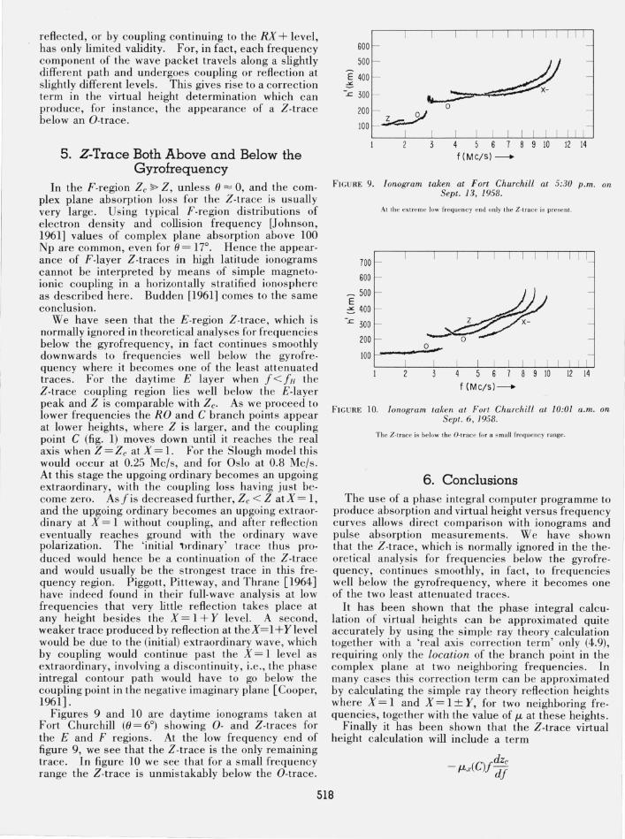
Figures 9 and 10 are daytime ionograms taken at Fort Churchill (() = 6°) showing 0- and Z-traces for the E and F regions. At the low frequency end of figure 9, we see that the Z-trace is the only remaining trace. In figure 10 we see that for a small frequency range the Z-trace is unmistakably below the O-trace.

600

500

E 400 :::s

-J:: 300

200

100

f (Me/5) __

FIGURE 9. lonogram taken at Fort Churchill at 5:30 p.m. on Sept. 13, 1958.

700

600 _ 500 E ::: 400

-:c 300

At the extreme low frequency end only the Z-trace is prese nt.

200

1001------

f (Me/5)--

FIGURE 10. tonogram takell at Fort Churchill at 10:01 a.m. all Sept. 6 , 1958.

The Z-Irace is below the O-trace for a smaU freque ncy range.

6. Conclusions The use of a phase integral computer programme to

produce absorption and virtual height versus frequency curves allows direct comparison with ionograms and pulse absorption measurements. We have shown that the Z-trace, which is normally ignored in the the­oretical analysis for frequencies below the gyrofre­quency, continues smoothly, in fact, to frequencies well below the gyrofrequency, where it becomes one of the two least attenuated traces.

It has been shown that the phase integral calcu­lation of virtual heights can be approximated quite accurately by using the simple ray theory calculation together with a 'real axis correction term' only (4.9), requiring only the location of the branch point in the complex plane at two neighboring frequencies. In many cases this correction term can be approximated by calculating the simple ray theory reflection heights where X = 1 and X = 1 ± Y, for two neighboring fre­quencies, together with the value of f-t at these heights.

Finally it has been shown that the Z-trace virtual height calculation will include a term

dzc - f-tx( C)/ d/

518

which in some cases may be sufficient to produce a Z-trace at a lower virtual height than that of the O-trace.

The 'real axis correction term ' is usually more sig­nificant in the E region than in the F region, where it is doubtful whether it wo uld be an important factor in explaining the overes timation of heights in electron density profiles whic h has sometimes led to a crossing over of 'topside' and 'bo ttomside' F-region profiles.

This communication is published by kind permis­sion of the Director of the D.S.I.R. Radio Research Station. The ionograms for Fort Churchill are pub­lished by permission of the World Data Centre for the ICY in Slough. The author is, indebted to Mr. W. R. Piggott for valuable discussions in the later stages of this work, and in particular for pointing out the existence of the E-region Z-traces for high latitude stations.

(Pape r 69D4-487)

519

7. References Barron, D. W., and K. G. Budden (1959), The nume rical so lution of

diffe re nti al equ a tions the re flec tion of long radio waves fro m the ionosphe re, Ill , Proc. Roy. Soc. A249, 387.

Budde n, K. G. (1955), Th e numeric al solution of diffe rential eq ua. tions governing refl ec tion of long radio waves from the ionosphe re, Proc. Roy. Soc. A227, 516.

Budden, K. G. (1961), Radi o waves in the ionosphere (Ca mbridge University Press).

Cooper, Elisabeth (1961), The properties of low freque ncy radio waves reflected from the ionosphere, calculated by the phase integral me thod, J. Atmospheric Terres t. Phys. 22, 122.

Deeks, D. G. (1964), D·region electron distributions in middle lati. tudes deduced from the re flection coefficients of long radio waves (private communications).

Johnson, F. S. (editor) (1961), Satellite environme nt handbook, pp . 28 and 40 (S tanford University Press).

Piggott, W. R. , M. L. V. Pitte way, and E. V. Thrane (1964), The numerical calculation of wave·fie lds , reflec tion coeffi cie nt s a nd polarization for long radio waves in the lower ionosphere, II , Phil. Trans . Roy. Soc. A (i n press).

Piggott, W. R., and E. V. Thra ne (1964), The elec tron de ns ities in the £. a nd D·regions deduced from studies of radio wa ve propa. ga ti on, J. AtmoS I)heri c Terres t. Ph ys . (in press) .

Pitte way, M. L. V. (1964), The nume rical calc ul ation of wave fi elds , refl ection coeffi cie nts and polarizations for long radio waves III

the lower ionos phe re, 1, Phil. Trans. Roy. Soc. A (in press) .