David R. Sallee

APPROVED: Paul F. Hudak, Major Professor Earl Zimmerman, Committee Member Douglas Elrod, Committee Member Harry Jacobson, Committee Member Kenneth Gee, Committee Member Reid Ferring, Chair of Department of Geography Warren Burggren, Dean of College of Arts and Sciences C. Neal Tate, Dean of the Robert B. Toulouse School of Graduate Studies

USE OF GEOGRAPHIC INFORMATION SYSTEMS AND INFRARED-TRIGGERED

CAMERAS TO ASSESS WHITE-TAILED DEER (Odocoileus

virginianus) HABITAT IN DENTON COUNTY, TEXAS

David R. Sallee, B.S., M.E.

Thesis Prepared for the Degree of

MASTER OF SCIENCE

UNIVERSITY OF NORTH TEXAS

August 2002

Sallee, David R., Use of geographic information systems and infrared-triggered

cameras to assess white-tailed deer (Odocoileus virginianus) habitat in Denton County,

Texas. Master of Science (Geography), August 2002, 106 pp., 12 tables, 25 figures,

references, 75 titles.

This study utilized geographic information systems, remote sensing, and infrared-

triggered cameras to assess white-tailed deer habitat in Denton County, Texas. Denton

County is experiencing tremendous growth in both population and development. Despite

their presence here historically, white-tailed deer were all but extirpated by the beginning

of the 20th century, and there are no data available which support their presence in

Denton County again until the 1980’s. This study attempts to equate the increase in

white-tailed deer population to Denton County’s transformation from an agricultural to

an urban economy and lifestyle. Eighteen sites were chosen throughout the county to

research the following metrics: geology, soils, landcover, landscape ecology, streams,

shorelines, land use, population, roads, structures, and census methods.

ii

ACKNOWLEDGEMENTS

I would like to thank the members of my committee, Dr. Earl Zimmerman, Dr.

Douglas Elrod, Dr. Harry Jacobson, Kenneth Gee, and especially my major professor Dr.

Paul Hudak, for their guidance, assistance, and support.

A special thank you goes to my family. None of this would have been possible

without the constant understanding, support and encouragement of my wife, Kris and my

daughters, Davi and Shelby.

Thanks are also extended to Bruce Hunter and Chris Miller for their technical

assistance, and to the many property owners/agents for granting me access to their

property. Finally, thanks is extended to the many students, professors and staff of both

the Department of Geography and the Department of Biological Sciences for their

assistance in the completion of my graduate studies.

iii

TABLE OF CONTENTS

Page LIST OF TABLES……………………………………………………………………iv LIST OF FIGURES………..……………………………………………………….…v Chapter

1. INTRODUCTION……………………………………………..…………...…1

2. BACKGROUND & LITERATURE REVIEW……………………………….4

Study Animal Historical Background Geology Soils Food and Cover Water Space Landscape Ecology Geographic Information Systems and Satellite Imagery Census Methods

3. METHODOLOGY…………………………………………………………..42

Study Area Geology Soils Land Cover Landscape Ecology Streams & Shoreline Land Use Population, Roads, & Structures Census Methods

4. RESULTS & DISCUSSION…...……………………………………………76 5. CONCLUSIONS………………………………………………………….…85

APPENDICES…………………………………………………………………………...91 LITERATURE CITED………………………………………………………………....101

iv

LIST OF TABLES

Table Page 1. Farmed acreage and number of farms per crop for years 1980 and 2000. 54 2. Agricultural crops per research site. 54 3. Geologic formations in Denton County by research site. 55 4. Soil orders in Denton County by research site. 55 5. UTM landcover reclassification for 1988 and 1999 in 7 landcover classes. 56 6. 1999 UTM landcover reclassification for Denton County. 57 7. Patch metrics. 58 8. Landscape metrics. 59 9. Habitat metrics per research site – water. 60 10. Habitat metrics per research site – space. 61 11. Number of white-tailed deer per research site and census method. 62 12. White-tailed deer sign per research site. 62

v

LIST OF FIGURES

Figure Page

1. Denton County boundary. 31

2. White-tailed buck, Site 10, Roanoke. 32

3. Range Map of White-tailed Deer Subspecies. 33

4. 1945 Range Map of White-tailed Deer in Texas. 34

5. Geologic Map of Denton County, Texas. 35

6. Physiographic Regions of Denton County, Texas. 36

7. Soils Map of Denton County, Texas. 37

8. Soil Horizon Symbols. 38

9. Homogeneous vs. Heterogeneous Fields. 39

10. Edge in patchwork landscape. 39

11. Interspersion. 40

12. Fragmentation. 41

13. Research Sites. 63

14. 1988 landcover. 64

15. 1999 landcover. 65

16. Change in landcover from 1988 - 1999. 66

17. Stream density. 67

18. Shoreline density. 68

19. 1990 population density. 69

20. 2000 population density. 70

21. Site 1, Isle du Bois and white-tailed deer. 71

22. Site 3, Bolivar and white-tailed deer. 72

23. Site 5, Stony and white-tailed deer. 73

24. Site 9, Flower Mound and white-tailed deer. 74

25. Site 14, Navo and white-tailed deer. 75

1

CHAPTER 1

INTRODUCTION

The four components of wildlife habitat are food, cover, water, and space (Gee

et al. 1994). Denton County, like much of the present day Cross Timbers and Prairies

ecological regions of North-Central Texas, has limited habitat for white-tailed deer

(Odocoileus virginianus). Despite this limited habitat, the area seems to be

experiencing a tremendous population growth of white-tailed deer. Today, more and

more people are experiencing white-tailed deer “sightings” throughout the county. This

is interesting for two reasons. First, despite having been here historically (Anon. 1945),

data for white-tailed deer cannot be located to support the presence of the species in the

county for most of the twentieth century, except for one account of a deer being killed

near Hebron, in the early 1950’s (Skipworth 2000). An interview with M.R. McNatt

(2001), revealed, that despite living in and around the county for all of her 93 years, she

had never heard of any white-tailed deer being seen and could not believe they are here

now. She and her husband, along with friends and family, spent much of their time

fishing on the streams and sloughs in the Trinity River drainage area. When asked if

she could elaborate, she said that if there had been white-tailed deer in this area during

the 1930s, people would have eaten them. Ed Pauls (1999), co-author of Soil Survey of

Denton County, said that when he and Alan Ford were driving and walking the entire

county, in the process of sampling the soils, during the 1960’s they did not see deer nor,

2

signs of deer with the exception of two tracks in the bottom of Clear Creek, northwest

of Bolivar. The first documented sightings were in the early 1980’s, and now these

sightings are fairly common. In April of last year, nine deer were observed foraging on

forbs (Gee et al. 1994; Lambert and Fulbright 1998; Lyons et al. 1996), within 100

yards of highway 114, about 5:30 PM.

Second, the numbers of white-tailed deer are increasing despite a huge growth

in both land development and human population. The cities of Denton, Lewisville, and

Carrollton are developing to their limits and beyond, while the small communities

around Lakes Grapevine and Lewisville are experiencing tremendous growth. Flower

Mound is showing a growth rate exceeding 200%, and in the eastern part of the county,

Frisco has grown nearly 500% in the last ten years (Census 2000). The area and

communities adjacent to Lake Ray Roberts are growing and may soon see similar

growth as the communities around the older lakes in the county are now experiencing.

The property in the southwest region of the county is also developing rapidly because

of Alliance Airport and Texas Motor Speedway.

It is my hypothesis that the fragmented landscape associated with Denton

County’s transformation from an agricultural to a more urban/metropolitan economy

and lifestyle provides habitat conducive to white-tailed deer. Where there used to be

great expanses of monoculture cropland and improved pasture, each year farms get

smaller and much more fragmented (Wilkins et al. 2000; Phillips 1999; Higginbotham

and Kroll 1992). This leaves much of Denton County in a fallow state and results in

An increasing number of acres of rangeland and shrub land becoming adjacent to

3

existing riparian zones. This adjacency expands the size and scope of suitable habitat,

and oftentimes connects that habitat with existing woodlots and/or agricultural crops

utilized by white-tailed deer. The optimum percentage of wooded areas for white-

tailed deer habitat in the Cross Timbers is probably in the range of 40-60%, with

patchy, irregularly shaped openings generally less than 180 m (200yards) in width (Gee

et al. 1994). With this in mind, human manipulation on a landscape or county scale and

lack of manipulation on a patch or parcel scale of much of Denton County has, in many

ways, improved its quality as white-tailed deer habitat.

4

CHAPTER 2

BACKGROUND & LITERATURE REVIEW

Study Area

The study area consists of Denton County (Figure 1), extending from Cooke and

Grayson Counties on the north to Tarrant and Dallas Counties on the south, and from

Wise County on the west to Collin County on the east. The area, which covers almost

2331 km2 (900 mi2), is made up of gently rolling hills laced with stream systems,

draining toward the Trinity River, Lake Ray Roberts, Lake Lewisville, and Lake

Grapevine. There are several small communities and two major cities including Denton,

which is the county seat and has a population of nearly 75,000, and Lewisville, which has

a population of nearly 60,000 (Census 2000). The county has an altitude range of 157 m

to 257m (515 ft to 844 ft). The January mean minimum temperature is 16.67 o C (30o F),

the July mean maximum temperature is 52.22 o C (94o F), and the average annual rainfall

is 94.74 cm (37.3 inches) (Ramos 1998).

Study Animal

The white-tailed deer (Figure 2) is named for its most distinctive feature, the large

white tail that is often all one sees as the animal bounds away through the forest

understory or tall grass. The body size of the white-tailed deer of north-central Texas,

Odocoileus virginianus texanus, is small in comparison to other subspecies and

5

especially when compared to other members of the deer family (Davis and Schmidly

1994). The external measurements of the average male are as follows: total length,

1,800 mm; tail, 300 mm; and hind foot, 450 mm. Females are slightly smaller (Davis

and Schmidly 1994).

The color of the white-tailed deer’s upper body and sides changes through the

seasons from a reddish-brown in summer to buff or gray in winter. Its ventor and throat

are always white. A fawn’s coat is similar to that of an adult buck or doe but has

several white spots, which gradually disappear when the fawn is 3 to 4 mos. old. Males

grow a new set of antlers every year, shedding the old ones after the breeding season

ends.

In Denton County and the North-Central Texas area, reproduction generally

takes place in early November, but can occur earlier or later. One or two fawns are

born after a 7-mo. gestation period. White-tailed deer are the most abundant large

game species in North America, and Texas is estimated to have three to four million,

the largest number of any state.

Historical Background

It is difficult to find literature on white-tailed deer that doesn’t include some

comment on their adaptability and other enduring qualities. What most people don’t

realize is just how long have they been enduring and adapting. White-tailed deer is a

member of the order Artiodactyla, family Cervidae, and genus Odocoileus (Rue 1997),

and has existed approximately 2.5 million years. The first known members of the order

6

Artiodactyla, known as Diacodexis, were rabbit-sized and date back to the early Eocene

Epoch (Halls 1984). Due to their adaptability, not only did they outlast many of the

related and unrelated species and genera that evolved during their time (Rue 1997),

they have survived a number of selection pressures and outlasted many now extinct

predators.

There are four subspecies of white-tailed deer in Texas. A map by Rue (1997)

illustrates the ranges of these subspecies (Figure 3). Although two of the subspecies are

near the area of Denton County, there is a sizable gap between the two. The Texas

whitetail, Odocoileus virginianus texanus, is found in western Texas, Oklahoma,

Kansas, southeastern Colorado, eastern New Mexico, and the northern portion of

Mexico. This subspecies, occurs just west of the study area. The Kansas whitetail,

Odocoileus virginianus macrorus, is found in eastern Texas, Oklahoma, Kansas,

Nebraska, Iowa, Missouri, Arkansas, and Louisiana and appears to range just east of the

study area. In Principal Game Birds and Mammals of Texas by the Texas Game, Fish,

and Oyster Commission (1945), a map illustrating the range of white-tailed deer shows

the nearest concentrations of any measurable size to be in western Wise County and

along the Red River in Montague and Cook Counties (Figure 4).

The white-tailed deer’s modern history is equally remarkable (Halls 1984),

where it is still demonstrating endurance and adaptability. In 1909, naturalist E.T.

Seton, in his book Lives of Game Animals, attempted to estimate the population of

white-tailed deer in North America. He based his work on the writings of the earliest

explorers, naturalists, and hunters (Rue 1997) and was able to illustrate his findings on

7

a map. His estimate of late-prehistoric/early-historic white-tailed deer range is fairly

consistent with the range of the modern white-tailed deer, as established by Rue (1997).

Throughout the history of North America, white-tailed deer have played a vital

role in the lives of Native Americans and settlers alike. Even with bison, moose, elk,

black bear, numerous small game, fish, and birds available in many parts of white-

tailed deer range, deer were the most widespread principle source of meat for Native

Americans (Halls 1984). The Sioux, who were Plains Indians known for their

dependency on the buffalo, called the white-tailed deer “tahca” or “tahinca,” meaning

“the true meat, the real meat” (Halls 1984). Besides utilizing deer as a food resource,

Native American relied on white-tailed deer for clothing, including leggings, shawls,

dresses, sashes, shirts, robes, skirts, headware, and mittens (Halls 1984; Bauer 1993;

Rideout 1991).

Exploration and settlement of the American frontier wouldn’t have come about

as fast or as safely without the white-tailed deer. One thing which makes that fact so

well understood is the realization that colonists and exp lorers utilized the skins and

meat of the white-tailed deer extensively, often trading deer hides among trappers,

frontier scouts, Indian scouts, and others (Hood 1998). Describing the mostly

uncharted Midwest in 1785, English naturalist Thomas Pennant wrote of a …“plain rich

in woods and savannas, swarming with Bisons or buffaloes, Stags, and Virginia Deer

… from the great lakes of Canada, as low as the gulph of Mexico; and eastward to the

Apalachian” (Halls 1984). U.S. Army Captain R. Marcy (1859) wrote in his travelogue

of the Southwest of seeing thousands of deer daily and herds of one to two hundred

8

being common spectacles. Dodge (1877) reported having seen about 1,000 whitetails

in a wintering herd in Texas (Halls 1984). It is unclear if the previous examples took

place near the location of Denton County, but it is possible because lush vegetation in

the Eastern Cross Timbers, Blackland and Grand Prairies, and along all of the many

streams, made this area prime habitat for white-tailed deer and many other species.

Archaeological finds have revealed their presence here (Yates and Ferring 1986), and

just like today when listed among all other game species, white-tailed deer were at the

top. This gives the impression they were the most abundant and/or the most important

species to settlers, just as they had been to Native Americans.

Texas Parks and Wildlife reports that deer were so much a part of early Texans’

lives that indiscriminate slaughter by commercial meat and hide hunters, as well as

ignorance of the deer’s habitat requirements, almost resulted in the animal’s

extermination by the end of the 19th century (Anon. 1945). According to Texas Parks

and Wildlife, one trapper near Waco is said to have shipped approximately 75,000

deerskins from 1844 through 1853 (Halls 1984; Hood 1998). In 1881, Texas adopted a

5-mo. closed hunting season, and in 1909 issued its first hunting license. In 1919, 5

game wardens were hired to patrol the entire state. Just as it did during prehistoric

times, the white-tailed deer has adapted and endured Indians, settlers, commercial

hunters, indiscriminate clearing and farming, overgrazing, droughts, disease, and

urbanization.

Geology

There are 13 different geologic formations and members (Barnes 1991), in

9

5 geologic groups, in 4 geologic series (Scoggins 1999), within the boundaries of

Denton County. The bedrock formations of the Cretaceous Series strike north-south

and dip eastward, with the oldest on the west, at 100+ million yrs old, and the youngest

on the east, at approximately 80 million yrs old. There are also three formations made

up of alluvium and windblown deposits (Barnes 1991) of the Pleistocene and Recent

Series (Scoggins 1999), deposited on bedrock along Denton Creek, Hickory Creek,

Clear Creek, Little Elm Creek, Panther Creek, Stewart Creek, Indian Creek, and the

Elm Fork of the Trinity River (Figure 5).

The Lower Cretaceous Series, which closely correlates to the “Grand Prairie”

Physiograhic Belt (Figure 6), includes a mixture of limestones, clays, and marls

(Winton 1925), which constitute parent material for loam (Alfisols), to gravelly/clay

loam (Mollisols), to clay (Vertisols). These soils, which have an average slope of 3

percent, are found on ridges, side-slopes, and in valley-fill areas. They comprise 23

percent of the area of Denton County and are used mostly for range, with some suitable

for pasture and crops (Ford and Pauls 1978).

The Upper Cretaceous Series, which closely correlates to the ”Eastern Cross

Timbers” and “Blackland Prairies” Physiographic Belts (Figure 6), includes the

Woodbine Formation, Eagle Ford Formation, and Austin Chalk, which are parent

material for fine sandy loam (Alfisols) to clay to silty clay (Vertisols) soil. These soils

account for more than 50 percent of the county and are used for crops, range, and

pasture, rating from good to medium to poor depending on location. There is an

average of 4 percent slope, with the least being zero and the maximum at 15 percent

10

(Ford and Pauls 1978). Where the dominant vegetation is Eastern Red Cedar

(Juniperus virginianus), the contrast between the “very white” Austin Chalk and the

underlying black-colored Eagle Ford Shale is striking. The Eagle Ford Formation,

consisting of a soil called “Black Gumbo,” supported mainly tall grasslands. The

Woodbine Formation is an iron-rich, sandy soil where the dominant vegetation is Post

Oak (Quercus stellata).

The Pleistocene Series (Scoggins 1999) is primarily fluviatile terrace deposits of

mixed origin and is the parent material for fine sandy loam (Alfisols) to clay loam

(Mollisols) to clay (Vertisols) to silty clay (Inceptisols) soils. These soils, which make-

up 8 percent of the total and have only moderate slope, are mainly pasture with some

designated for wildlife and range (Ford and Pauls 1978). The Recent Series (Scoggins

2000) is alluvium along the flood plains, and is the parent material for a group of soils

ranging from sandy loam (Entisols) to clay (Vertisols) to silty clay (Mollisols) soils.

These soils, which have very little slope, are flooded occasionally to frequently and

comprise 12 percent of the county. Their use is mostly for crops, pasture, range, and

wildlife (Ford and Pauls 1978). These alluvial deposit areas will be referred to as

riparian zones in later sections.

Soils

Alfisols (Figure 7) are more strongly weathered than the other soils and are

formed in cool to hot humid areas. They are also found in the semiarid tropics and

Mediterranean climates. Most often, Alfisols develop under native deciduous forests,

11

although in some cases grass savanna is the native vegetation. Alfisols are

characterized by a subsurface diagnostic horizon in which silicate clay has accumulated

by illuviation (Brady and Weil 1999). A typical Denton County Alfisols pedon (Figure

8) appears as follows: A 1:0-15 cm (0-6 in) of brown fine sandy loam, dark brown

moist; B 21:15-43 cm (6-17 in) of yellowish red clay, yellowish red moist; B 22t:43-69

cm (17-27 in) of yellowish red clay, yellowish red moist; B 3:69-86 cm (27-34 in) of

mottled yellowish red, strong brown, and red sandy clay and; C r:86-152 cm (34-60 in)

of strong brown and yellowish red brittle fractured sandstone, with 2.5-10 cm (1-4 in)

strata of strong brown, yellowish red, red, and gray shaly clay (Ford and Pauls 1978).

Entisols (Figure 7) are weakly developed mineral soils without natural horizons,

or with only the beginnings of such horizons. Most have an ochric epipedon and a few

have human-made anthropic or agric epepidons. Soil productivity ranges from very

high in certain Entisols formed in recent alluvium, to very low for those forming in

shifting sand or on steep rocky slopes (Brady and Weil 1999). A typical Entisols pedon

(Figure 8), of Denton County, appears as follows: A 1:0-13 cm (0-5 in) of brown fine

sandy loam, dark brown moist; C 1:13-53 cm (5-21 in) of brown fine sandy loam, dark

brown moist; C 2:53-107 cm (21-42 in) of brown sandy clay loam, dark brown moist

and; C 3:107-168 cm (42-66 in) of brown sandy clay loam, dark brown moist (Ford and

Pauls 1978).

The main soil- forming process affecting Vertisols (Figure 7) is the shrinking

and swelling of clay as these soils go through periods of drying and wetting. Vertisols

have a high content of sticky, swelling and shrinking-type clays to a depth of one meter

12

or more. Most Vertisols are dark, even blackish in color, to a depth of one meter or

more. The native vegetation is usually grassland (Brady and Weil 1999), where deep

root mats are formed.

A typical Denton County Vertisols pedon (Figure 8) appears as follows: A 1:0-

15 cm (0-6 in) of grayish brown clay, dark grayish brown moist; AC 1:15-76 cm (6-30

in) of grayish brown clay, dark grayish brown moist; AC 2:76-124 cm (30-49 in) of

grayish brown silty clay, dark grayish brown moist and; C:124-315 cm (49-70 in) of

grayish brown marly silty clay, dark grayish brown moist (Ford and Pauls 1978).

The principle process in the formation of Mollisols (Figure 7) is the

accumulation of calcium-rich organic matter, largely from the dense root systems of

prairie grasses, to form the thick, soft Mollic epipedon that characterizes soils in this

order. This humus-rich surface horizon is often 60 to 80 centimeters in depth and high

in calcium and magnesium (Brady and Weil 1999). A typical Mollisols pedon (Figure

8), of Denton County, appears as follows: A 1:0-33 cm (0-13 in) of dark grayish brown

clay loam, very dark grayish brown moist; B 21:33-51 cm (13-20 in) of grayish brown

clay loam, dark grayish brown moist; B 22ca:51-79 cm (20-31 in) of light olive brown

clay loam, olive brown moist; B 3ca:79-91 cm (31-36 in) of light brownish gray silty

clay loam, grayish brown moist and; R:91-112 cm (36-44 in) of hard, fractured

limestone rock coated with calcium carbonate (Ford and Pauls 1978).

In Inceptisols, the beginning or inception of profile development is evident, and

some diagnostic features are present. However, the well defined profile characteristics

of soils thought to be more mature have not yet developed. The natural productivity of

13

Inceptisols varies considerably (Brady and Weil 1999), from some of the best to poor.

A typical Denton County Inceptisols pedon (Figure 8) appears as follows: A 1:0-15 cm

(0-6 in) of pale brown silty clay, brown moist; B 2:15-58 cm (6-23 in) of light

yellowish brown silty clay, yellowish brown moist; B 2ca:58-142 cm (23-56 in) of light

yellowish brown silty clay, yellowish brown moist and; C:142-203 cm (56-80 in) of

brownish yellow silty clay, yellowish brown moist (Ford and Pauls 1978).

As stated above, habitat quality for white-tailed deer is significantly correlated

with soil quality. Soil fertility will directly and substantially affect the quality of

habitat (McMullin 2000; Miller and Marchinton 1995). The carrying capacity of

various ranges will differ according to the types and abundance of vegetation, types and

mineral content of the soil, the classes of domestic livestock present, the range

management practices in effect, and the classes of wildlife species. Research has

indicated the poor quality of the white-tailed deer in Florida is attributable to the poor

(low mineral content) soils (Brothers and Ray 1998). Following soil quality, habitat

type, successional stage, and amount of habitat interspersion or edge have the greatest

impact on deer habitat quality (McMullin 2000).

White-tailed deer, like any other animal, must have a proper level of nutrition

available throughout the year in order to maintain body condition and reproduce

efficiently (Baccus et al 1998). Calcium and phosphorous are required for bone and

antler growth and for lactation (Richardson date unknown). The diet should contain

12% to 18% protein and a calcium/phosphorous ratio of 2:1 (Brothers and Ray 1998).

White-tailed deer, especially males, go through dramatic physiological, morphological,

14

and endocrine changes during the year. Because of this, they have changing nutritional

requirements. The protein requirement for a buck in May is far greater than the amount

needed in December, since antlers are growing in May, but not in December (Handley

1999). Females have greater requirements during gestation in Spring and during

lactation in Summer.

A widely accepted but unproven concept in white-tailed deer habitat

management is that plant diversity plays a key role in nutrition. In theory, deer in

diverse habitats can switch from one food to another as one plant declines in nutritional

quantity and another increases in quantity during seasonal cycles. Therefore, deer in

areas of diverse habitat are able to maintain a relatively constant level of nutrition

compared to deer in less diverse habitats (Lambert and Fulbright 1998). It is often true

that the soils most productive for the growth of grasses also produce the widest variety

and best growth of brush species and forbs beneficial to deer. Not only is food

available in abundance from these thick brush areas, but also the cover is usually the

best available. A good example of the best soils would be bottomland soils adjacent to

rivers and streams (Brothers and Ray 1998).

Food and Cover Requirements (Natural Vegetation)

The three basic forage classes preferred by white-tailed deer are forbs, browse,

and grasses/grasslikes. Forbs include all flowering herbaceous plants that are not

grasses or grasslikes. Browse refers to perennial woody vegetation including their

fruits. Trees, shrubs, and many vines fall into this category. When referring to a type

15

of plant, the terms “woody” and “browse” are synonymous (Gee et al 1994).

In Denton County, the Blackland Prairie (Figure 6) is all but lost because of

plowing, overgrazing, and urban sprawl. Today this area is growing in population with

a continuous wave of new homes and strip malls. The only part of the Blackland

Prairie where some forest has survived intact is on the escarpments. An escarpment, or

scarp, is the exposed offset in a strike-slip fault. Along the escarpments the woods are

fifteen to thirty feet tall and composed mostly of Eastern Red Cedar (Juniperus

virginiana) and Ashe Juniper (Juniperus ashei) with ornamental trees such as Mexican

Buckeye (Ungnadia speciosa), Texas Buckeye (Aesculus arguta), Hercules Club

(Zanthoxylum clava-hercules), and Eve’s Necklace (Sophora affinis) (Wasowski and

Wasowski 1997; Cooper 1997). Even though the areas where the wooded escarpments

are adjacent to crops and streams are good habitat, the overall numbers of white-tailed

deer in the Blackland Prairies in Denton County should be minimal because of the

relative small acreages of habitat, fragmentation of these acreages, and the enormous

human population growth.

What is left of the Eastern Cross Timbers (Figure 6) is probably much the same

as it was when settlers first arrived in this area. Much of this sandy area has been

cleared for farming and ranching, except where slope has prevented and is dominated

by Post Oaks (Quercus stellata), but Blackjack Oak (Quercus marilandica), American

Elm (Ulmus americana), Texas Mulberry (Morus microphylla), and Bois d’arcs

(Maclura pomifera) are also found. Greenbriar (Smilax bona-nox) is the main

understory plant with some Poison Oak (Toxicodendron radicans), Rusty Blackhaw

16

(Viburnum rufidulum), Possomhaw (Ilex deciduas), Smooth Sumac (Rhus glabra),

Coralberry (Symphoricarpus orbiculatus), and Arkansas Yucca (Yucca arkansana)

(Wasowski and Wasowski 1997; Cooper 1997). Early travelers through this area

referred to the Cross Timbers as an impenetrable barrier. Areas in and adjacent to the

Elm Fork riparian zone and many of the hills that border it remain difficult to

impossible to ride a horse through except where the understory has been cleared or it

has been grazed by domestic livestock.

The Grand Prairie (Figure 6), once a mid-grass prairie with Little Bluestem

(Andropogon scoparius) dominating, along with Indian Grass (Sorghastrum nutins) and

Sideoats Grama (Bouleloua curtipendula) ( Rosenkrantz and Koelsch, Dyksterhuis

1946; Wasowski and Wasowski 1997; Cooper 1997), consists of improved pasture,

feed crops, fields with a mixture of native and non-native grasses, and fields that have

gone fallow.

Today, woody species are growing on much of the uplands of the Grand Prairie,

but they are not trees that are native to the area. They are species more likely to be

found on the Edwards Plateau: Texas Ash (Fraxinus texensis), Escarpment Live Oak

(Quercus fusiformis), Ashe Juniper (Juniperus ashei), Texas Redbud (Cersis

Canadensis var. texensis), and Mexican Buckeye (Ungnadia speciosa) (Wasowski and

Wasowski 1997; Cooper 1997). Observations show an abundance of Honey Mesquite

(Prosopis glandulosa) and Prickly Pear cactus (Opuntia spp. complex) in fallow fields

and shrub land of the Grand Prairie Region.

Riparian zones are mixed with hardwood and softwood trees. Pecan (Carya

17

illnoensis), Black Hickory (Carya texana), Hackberry (Celtis spp. complex),

Cottonwood (Populus deltoids), Red Oak (Quercus nuttallii), Post Oak (Quercus

velutina), American Elm (Ulmus Americana), Cedar Elm (Ulmus crassifolia), and

Black Willow (Salix nigra) are present in abundant numbers, while the understory is

made up of Greenbriar (Smilax bona-nox), Poison Ivy (Toxicodendron radicans),

Smooth Sumac (Rhus glabra), Soapberry (Sapindus drummondii), Carolina Buckthorn

Rhamnus caroliniana), Mexican Plum (Prunus mexicana), Possumhaw (Wasowski and

Wasowski 1997; Cooper 1997). These riparian zones consist of deposited and terraced

sandy and clayey soils which are high in nutrients. What vegetation might be found

depends on how often a location floods and how long before the waters subside

Food and Cover Requirements (Agricultural Vegetation)

The Texas Agricultural Extension Service suggests that food selection by white-

tailed deer is largely an innate behavior (Spalinger et al 1997), and white-tailed deer

consume more or less the same amount of grass across all seasons, more forbs in spring

and less in winter, and more browse in fall and winter and less in spring (Lyons et al

1995). Texas Parks and Wildlife biologists agree that white-tailed deer are very

adaptable and often adopt food sources that are planted as cultivated crops. Deer prefer

crops such as peanuts, wheat, oats, corn, grain sorghum, truck crops and vegetable

gardens (Dillard 1994).

Denton County has experienced a decrease in farmed acres and in the size of

18

each farm, but an increase in the number of farms, in recent years. From 1987 to 1997,

Denton County farms have increased in numbers from 1469 to 1782, and decreased in

hectares (acres) per farm from 108 (266) to 83 (204). In 1997 there was still 146,785

ha (362,712 ac) farmed (USDA 1997). The eastern portion of the county consists of

the Blackland Prairie, where the crops are wheat, soybean, corn, and grain sorghum.

Wheat, soybean, and grain sorghum is also grown in the sandy soil of the Eastern Cross

Timbers, as well as peanuts. In the remainder of the county, which is mostly in the

Grand Prairie, the farmers and ranchers grow wheat, grain sorghum, and some corn. In

Denton County, it is a common practice to rotate crops, and frequently the other crop is

hay. Because of its high yield, high protein, and high digestible nutrient level, many

farmers and ranchers are growing perennial Coastal Bermuda grass, for pasture and

hay. In 2000, Denton County farmers raised 19,829 ha (48,998 ac) of wheat, 5,685 ha

(14,047 ac) of grain sorghum, 488 ha (1,206 ac) of peanuts, and there were 1938 ha

(4,790 ac) of miscellaneous corn, barley, oats and soybean (Table 3). There were 7,527

ha (18,600 ac) of Sudan hay and 8,500 ha (21,000 ac) of Coastal Bermuda hay grown

in Denton County, in 2000 (English 2002).

Water Requirements

Water is seldom the limiting factor for white-tailed deer habitat, but Gee (1994)

states, “Like all animals, they require water to survive. Water is necessary for

important bodily functions such as metabolizing food for tissue and energy production,

temperature regulation, and waste excretion.” Deer drink from streams, rivers, springs,

19

lakes, and ponds (Figure 1). In addition to the above sources, white-tailed deer acquire

water from much of the food they consume. The amount of water deer require depends

on the climate, season, their particular activity, and the moisture content of their food

(Clancy and Nelson 1991, Halls 1984). Personal observations have shown that when

vegetation is lush, consumption of surface water is limited, and conversely, during

times of drought, they will stand chest-deep in a stock pond and drink water like cattle.

As noted above, Denton County is laced with the numerous streams of the Elm

Fork of the Trinity River drainage (Figure 1). These seasonal creeks and streams are

often dry in times of extended drought, but still hold water in deeper pools. The ones

draining into the Trinity from the west have their beginnings in Montague County,

while the headwaters of the ones draining from the east are in Grayson and Collin

Counties. The head of the Elm Fork of the Trinity is just a few km (mi) from the Red

River, in Cooke County. Lakes Ray Roberts and Lewisville have altered the original

course of the Trinity. Denton Creek flows into Lake Grapevine along its journey to the

Trinity. There is also excellent habitat in areas around the lakes. In addition to the

streams and lakes, there are numerous other sources of water in the way of ponds, stock

tanks, and springs, throughout the county.

Space Requirements

The carrying capacity of a particular area for wildlife is not only a function of

the availability of food, cover, and water, but is also controlled by the amount of

available space an animal requires. Space is a limiting factor when the combination of

20

range size and range quality is insufficient to maintain a viable deer population

(Dickson and Vance 1981; Gee et al. 1994). Home ranges can be expressed as the size

of an animal’s habitat or living area. The size of the home range is dependent on a

particular species’ needs and is a direct result of the behavioral nature, daily and

seasonal activity patterns, and movement. The size of the home range is modified by

shifts in population density, disturbances, and seasons. The space used by individual

deer varies greatly according to age, sex, and habitat characteristics (Gee et al 1994) but

there is a general consensus among many biologists, managers, and hunters that the

home range of white-tailed deer is approximately one square mile or 259 ha (640 ac).

The home range of each white-tailed deer overlaps the home range of other deer. Deer

may feed in seasonal patches, but return to their home range (Dickson and Vance

1981). During the breeding season, white-tailed bucks may cover as much as 13 km2 (5

mi2), but will return when it is over (Bauer 1993).

Where there were once great expanses of cropland and improved pasture in

Texas, each year the parcels get smaller and much more fragmented (Wilkins et al.

2000; Phillips 1999; Higginbotham and Kroll 1999). This is true for Denton County as

well. White-tailed deer prefer edge or the zone between two different types of habitat,

such as forest and field. An edge affords easy access to cover plus a variety of foods,

from grasses to forbs to browse. Patchworks, rather than vast expanses of a single type

of cover, would support the densest deer populations because they have the greatest

amount of edge habitat. By reducing the sizes and numbers of cropland and improved

pastures, there is a general increase in the number of fallow fields and edge habitat.

21

Many of these fields connect riparian zones, and/or agricultural fields with the few

remaining stands of hardwood forest. Denton County, like other counties in north

central Texas, has experienced tremendous growth in recent years. Much of the county

is developed into rural ranchettes, while other areas are turned into large residential

areas with greenbelts, golf courses, and man-made lakes and streams. Much of the

county lies dormant or fallow waiting to be developed. These trends may be

responsible for the recent increase in numbers of white-tailed deer in Denton County.

Landscape Ecology

Landscape ecology attempts to link ecological processes with spatial patterns,

and the fundamental unit is the patch. A patch is defined as a community or species

assemblage that is surrounded by areas with dissimilar communities (Smith 1997).

Two factors influence landscape: humans at small scale and topography at a broader

scale. Human influence is in the form of development of roads, plowed fields, and

structures (Newell 1996). Topography is regulated by the interactions of different

climatic and geologic processes.

Landscape is characterized by vegetation, and one can assume that if the

vegetation has a heterogeneous (Figure 9) or diverse distribution, then other (wildlife)

distributions are also heterogeneous (Smith 1997). Species diversity is a sign of good

habitat health. Questions regarding the amount and distribution of a patch within a

landscape can directly relate to population distributions of white-tailed deer and other

organisms (Smith 1997). The four landscape metrics that impact white-tailed deer as

22

evaluated in this research are 1) edge habitat, 2) riparian zones, 3) interspersion and 4)

fragmentation.

The transition area between forested areas and open land is known as “the edge”

(Figure 10). Many species, including white-tailed deer thrive in these areas because

they generally have more plant diversity including browse, forbs, and grasses (Gee et

al. 1994). According to the edge principle, the more edge in a given area the greater the

variety and abundance of wildlife (Dickson and Vance 1981). Generally, in north-

central Texas, white-tailed deer prefer openings intermixed with wooded areas rather

than large blocks of either one (Gee et al. 1994). White-tailed deer are not much more

fond of large stands of timber and brush than they are of large open fields. The

optimum percentage of each type of habitat depends on species composition and

distribution (Gee et al 1994). When forested areas include riparian zones and/or adjoin

croplands the quality of the edge is increased.

Riparian zones constitute some of the best habitat for white-tailed deer in

Denton County. According to the United States Department of Agriculture (1998), a

riparian zone is an area of trees and shrubs located adjacent to streams, ponds, lakes,

and wetlands. The vegetation in these buffer zones provides food and cover for

wildlife. The rich diversity of vegetation found in riparian zones fosters high species

richness and abundance. Many of the riparian zones in Denton County are bottomland

hardwood forests.

Bottomland hardwood forests not only offer quality habitat for white-tailed

deer, but also harbor a virtua l menagerie of wildlife. White-tailed deer populations are

23

healthier and attain greater densities in extensive river bottom habitats (Frentress

1986). Poteet et al (1996) reports riparian zones are an important part of the home

range of females and young males. A survey by the United States Fish and Wildlife

Service showed for the average stream in the United States, 273 species of birds, 45

species of mammals, 54 species of reptiles, 31 species of amphibians, 116 species of

fish, and innumerable invertebrates making their home in bottomland hardwood forests

(Frentress 1986, Anon. 1998). Connecting a riparian zone with existing vegetation,

such as a woodlot, benefits wildlife and aesthetics. Riparian areas also serve as

corridors between existing areas of habitat. There is also excellent habitat in many

areas adjoining the reservoirs, stock ponds, and springs throughout the county.

Besides providing food and cover for white-tailed deer and other wildlife,

riparian zones intercept sediment, nutrients, pesticides, and other materials in surface

runoff (Anon. 1998, Newell 1996). Woody plants adjacent to the stream lower water

temperature, slow out-of-bank-flows, and provide litter fall and other debris to aquatic

organisms. The roots of some vegetation aid in resistance to stream bank erosion

(Anon. 1998).

The edge was said to be the transition zone between forest and open land. This

transition zone can take on any shape and often lies in a straight line along a fence or

roadway. When the shape is irregular (Figure 11), it is referred to as interspersion

(Dickson and Vance 1981). There is a mixing or inter-digitation of feeding, loafing,

bedding, and cover areas. Interspersion is important to white-tailed deer and if it does

not occur, plants which provide food may be located too far from plants providing

24

protective cover (Dickson and Vance 1981). In Denton County, interspersion is

obvious in many parts of the Eastern Cross Timbers (post-oak belt). Interspersion

occurs naturally but can be created, such as the clearing of timber in “finger-shaped”

openings, which promotes the growth of shrubs, forbs, and grasses.

In a 1996 presentation in Kerrville by Texas A&M’s Department of Wildlife

and Fisheries Sciences, Dr. Bob Brown said, “The No. 1 threat to wildlife in Texas is

fragmentation.” Owner fragmentation is the break-up of rural properties into smaller

and smaller parcels (Wilkins et al 2000, Rollins 1999, and Newell 1996). Possible

causes of fragmentation are 1) declining agriculture economy, 2) an increasing number

of people seeking country property for commutes, retirement, or weekend retreats, 3)

federal inheritance tax laws which often force sales of portions of land, and 4) heirs

who choose to sell because of lack of interest in farming, ranching, or wildlife (Phillips

1999).

Habitat fragmentation (Figure 12) results from parceling off of property in such

a way that critical habitat is lost, resulting in the remaining habitat becoming isolated,

much the same way an island is isolated in a body of water. This effect is compounded

with the loss of corridors between patches of natural habitat (Newell 1966).

Fragmentation is the largest threat to habitat and to the wildlife using that habitat

(Wilkins et al. 2000). Most of the growth in land ownership has occurred in the 4-73 ha

(10-180 ac) parcel size, and inside the area formed between Dallas, Houston and San

Antonio, more than 65% of the tracts contain less than 73 ha (180 ac) (Wagner 2002).

Fragmentation rates vary across the state but seem to be influenced somewhat by

25

ecological region. The greatest increase in fragmentation, 3-25%, occurs in the

Blackland Prairie, Gulf Coast Prairies, and Edwards Plateau regions. Property size

seems to correspond to population, with an area generally east of a Fort Worth-San

Antonio line consisting of tracts averaging 61-202 ha (150-500 ac) each, compared to

tracts exceeding 202 ha (500 ac) generally west of that line (Wilkins et al 2000).

Is there a situation where fragmentation is a positive characteristic? For

example, based on personal observations and interviews with residents, much of

Denton County once consisted of large, homogenous, monocultures, where much of the

wildlife, and especially white-tailed deer, were confined to narrow riparian zones.

When large farms are broken up into smaller parcels, the amount of fence-line is

increased, which is quickly taken over by plants such as hackberry, bois d’arc, and

mesquite. This positive fragmentation results in a patchwork of fields where a variety

of crops are grown or no crops occur on many of them. Many tracts are absentee-

owned and someone leases them for grazing or hay rights. Others sit unattended for

long periods of time.

Geographic Information Systems and Remote Sensing

Geographic Information Systems (GIS) involves special hardware and software

that allow users to collect, store, retrieve, reorganize, analyze, and display data from the

real world (Congalton and Green 1992). An important attribute is the capability of the

GIS data from different maps and sources, such as field data, map data, and remotely

26

sensed images, to be registered together at the correct geographic location within a

common database, with a common map scale and map projection (McKnight and Hess

2000). GIS is used mainly in overlay analysis, where two or more layers of data are

integrated, and allows the user to visualize data in new ways that reveal relationships,

patterns, and trends not visible with other systems (Anon. 1999).

Geographic Information Systems mean many things to many people, and Nyerges

(1993) claims “GIS has a considerable potential for influencing environmental

modeling.” GIS is useful when dealing with single ownership over a smaller spatial

scale. An example of this situation would be a forest or district. It is also useful when

dealing with multiple and mixed ownerships over large spatial scales. An example of this

situation would be a stream’s watershed or county (Gregg 1994).

Remote sensing is any measurement or acquisition of information by a recording

device that is not in physical contact with the surface of the Earth. Common methods of

remote sensing include aerial photographs and orthophoto maps (McKnight and Hess

2000). An aerial photograph is one taken from any elevated point, but usually comes

from specially designed fixed-wing aircraft. Depending on camera angle the photographs

are classified as either vertical or oblique. A vertical photograph is one taken directly

below the aircraft, while an oblique photograph is taken at an angle less than 90o.

Orthophoto maps are multicolored, distortion-free photographic image maps. They are

prepared from digital representations of aerial photographs, and all distortions from

camera angle and relief have been corrected. This gives ortho-photographs the geometric

qualities, such as scale, of a map (McKnight and Hess 2000). Advances made in the field

27

of remote sensing have had a huge impact on Geographic Information Systems (Nyerges

1993).

Census Methods

Unlike domestic animals, white-tailed deer cannot be counted by using traditional

methods. Sample census methods, such as the Hahn, spotlight, aircraft, and fecal pellet are

used throughout the United States (Shult and Armstrong 1999; Demarais et al. 2000; Gee

2000; Dillard 1994). For years, the two methods used most often in Texas were the spotlight

(Rollins et al.1994) and aircraft (Hellickson 1999). Today there is a third method. The

infrared-triggered camera, according to Jacobson (2000), is more accurate and precise than

any other method.

The spotlight technique is as follows: (1) The census should begin well after dark

and takes place on a designated stretch of road. This section of roadway is pre-selected and

visibility is calculated prior to the census. It is important to survey the same stretch of road

and do it on approximately the same date each year. (2) Two people are in the back of a

vehicle, and with the use of spotlights, they count and classify (if possible) any deer seen.

Classification includes both sex and age. (3) Visibility is taken at .16 km (.10 mi) intervals

(Shult and Armstrong 1999) and when possible the census should consist of a line at least 16

km (10 mi) long. Texas Parks and Wildlife biologists, throughout much of Texas, including

Denton County, use this type of census not to establish a quantity but to illustrate a trend

from previous years. Dillard (1996) recommends that white-tailed deer surveys in the Cross

Timbers region be conducted during August and September. During this time period, bucks

are forming bachelor groups, and the fawns are moving with the does. In a comparison study

28

by Rakestraw and Silvy (1995), it was determined that spotlight surveys performed at night

were far more successful than similar surveys done in the morning and evening. Dale Rollins

(et al 1994) with the Texas Agricultural Extension Service, indicates that people conducting

spotlight surveys should be aware of how different habitats affect the census. In a study

performed by him and others, only an accuracy of 67-72% was achieved. Gee (2000) states

the accuracy and precision of spotlight surveys remain inconsistent across the range of uses.

Although some aerial surveys are performed using fixed-wing aircraft, most in this

part of the country are done using helicopters. The helicopter survey method is the most

popular method in South Texas (Hellickson 1999; Weishuhn 1997). This popularity is due to

the vast amounts of short, thin scrub brush found throughout South and West Texas, as well

as the relatively large areas that can be covered in a short amount of time. Weishuhn (1997)

makes the point that helicopter surveys are used in parts of North Texas, as well as the Hill

Country and Trans-Pecos regions. Unlike the spotlight survey, which is used to establish a

trend, helicopter surveys are designed to obtain the total number of bucks, does, and fawns

on a given tract of land, as well as approximate the age of the bucks (Hellickson 1999). From

the Wildlife Management Handbook, Weishuhn explains the census as follows: (1) The crew

should consist of a pilot and an experienced biologist-observer, and sometimes a second

observer. (2) Altitude varies with vegetation type. (3) Normal speed of helicopter is 30 m.p.h.

but depends on density of vegetation, wind, temperature and other factors. (4) The census

should be conducted during peak white-tailed deer movement, which is early morning

and late evening. (5) Winter surveys are best because counts are more accurate when there is

29

less vegetation. In a study performed by researchers at the Caesar Kleberg Wildlife Research

Institute, the effectiveness of a helicopter survey was only 23-69 % and rarely is it over

75 % (Heffelfinger 2000, Kroll and Koerth 2000).

Jacobson et al (1991) first used infrared-triggered cameras to study the effects of

baiting on white-tailed deer movement. They wanted to know if any of the radio-collared

deer (from a previous study) would show up at their bait sites. The results were staggering

because within a few days they had photographed every deer tha t had a home range, which

included bait sites. In 1992, he collaborated with Dr. James Kroll of Stephen F. Austin

University and his graduate students on a 2-year research study. When the study concluded

they found that they had photographed 30 of 30 radio-collared deer the first year, and 30 of

34 in 1993. It was also determined that they could identify individual bucks using body and

antler characteristics. In 1992 the photographs revealed 142 forked antlered bucks and 152 in

1993. After they had accounted for the fork-antlered bucks they, using photograph ratios,

could determine reliable population estimates of spikes, does, and fawns. When they added

these numbers to those of the fork-antlered bucks the result was a total population estimate

(Jacobson 2000). The total population estimate derived from studies of this nature became

known as the “camera estimate” (Walock et al. 1997). White-tailed deer management had

moved into a new era, and according to Kroll and Koerth (2000), it is possibly the most

exciting and important tool since radio telemetry, and the “single most important

breakthrough in deer management technology in the last 20 yrs.” Infrared monitors had been

used for years to monitor trails but only told part of the story. All one had was a record of an

event occurring when the beam was broken. It was not apparent what kind of animal broke

30

the beam, whether it was man or animal, or whether it was the same animal repeatedly

breaking the beam. Now all of those questions and more could be answered.

Before Jacobson performed his first study in 1991, others had begun to use infrared

cameras, but his study with Kroll in 1992 was the first time the cameras were used to perform

a wildlife census. According to Jacobson (2000), since that first census in 1992, the infrared-

triggered cameras out-performed spotlight counts, helicopter census, and even aerial infrared

census. As with all things there are some drawbacks. The success of a camera survey is “a

function of the ability to attract animals to bait. Factors such as familiarity with bait, mast

crop, and other food sources will influence success” (Demarais et al. 2000). In a study at the

Noble Foundation Wildlife Unit, the success rate wasn’t as good as was expected. But

according to Gee (2000), the skewed data were probably the results of a bumper acorn crop

and unusually mild winters of the past couple of years. Also non-target animals will

influence the overall success by eating the bait, using up the film, and/or scaring away the

target animals. Throughout the range of white-tailed deer, pictures of Racoon (Procyon

lotor), Eastern Fox Squirrel (Sciurus niger), Eastern Cottontail (Sylvilagus floridanus), and

Feral Pig (Sus scrofa) are common (Davis and Schmidly 1994), as well as wild turkey

(Meleagris gallopavo) and a multitude of other birds. In addition to White-tailed Deer, in the

United States infrared-triggered cameras have been used to monitor and census other species

of animals including, but not limited to, the Grizzly Bear (Ursus arctos) (Mace et al. 1994),

Black Bear (Ursus americanus) (Bowman et al. 1996), wild turkey (Meleagris gallopavo)

(Cobb et al. 1993), and Bobwhite Quail (Colinus virginianus) (Higganbotham 2001).

31

Figure 1. Denton County Boundary – 18 research sites with .8 km (.5 mi) radius

buffers. (1 mi = 1.6 km).

#

#

#

#

#

#

##

#

#

#

#

#

#

#

##

#

10 0 10 Miles

N

EW

S

32

Figure 2. White-tailed buck, Site 10, Roanoke, Texas.

33

Figure 3. Range Map of White-tailed Deer Subspecies.

34

Figure 4. 1945 Range Map of White-tailed Deer in north-central Texas.

Denton County

Present Range

Restocked Areas

35

Figure 5. Geologic Map of Denton County, Texas 18 research sites with .8 km (.5 mi) radius buffers. (1 mi = 1.6 km).

#

#

#

#

#

#

##

#

#

#

#

#

#

#

##

#

10 0 10 20 Miles

½ mile radius buffer

Research Site

N

EW

S

LEGEND Qal, Qt, Qu : alluvial and fluviatile deposits Kgw, Kfw, Kki, Kfd, Kpd, Kgm, : Limestone and Marl undivided Kwe, Kpp, Kdc, Kd Kwg : Woodbine Formation Kef : Eagle Ford Formation Kau : Austin Chalk Formation

36

Figure 6. Physiographic Regions

Grand Prairie Eastern Cross Timbers Blackland Prairie

Denton County

37

Figure 7. Soils Map of Denton County, Texas and 18 research sites with .8 km (.5 mi) radius buffers. (1 mi = 1.6 km).

#

#

#

#

#

#

##

#

#

#

#

#

#

#

##

#

1 0 0 1 0 M i l e s

SoilsCUMULIC HAPLUSTOLLS, FINE-LOAMY, MIXED, THERMICLITHIC USTOCHREPTS, LOAMY, CARBONATIC, THERMICOXYAQUIC HAPLUDERTS, VERY-FINE, MONTMORILLONITIC, THERMICTYPIC CALCIUSTOLLS, LOAMY-SKELETAL, CARBONATIC, THERMICTYPIC PELLUDERTS, FINE, MONTMORILLONITIC, THERMICUDERTIC HAPLUSTALFS, FINE, MONTMORILLONITIC, THERMICUDERTIC HAPLUSTOLLS, FINE, MONTMORILLONITIC, THERMICUDIC CHROMUSTERTS, FINE, MONTMORILLONITIC, THERMICUDIC USTIFLUVENTS, SANDY, MIXED, THERMICUDORTHENTIC HAPLUSTOLLS, FINE-SILTY, CARBONATIC, THERMICULTIC PALEUSTALFS, FINE, MIXED, THERMICWATER

Water.5 mile radius buffer

# Research Sites

N

EW

S

38

Figure 8. Soil Profile Symbols Monroe, J., R. Wicander. 2001. The Changing Earth. Brooks/Cole. Pacific Grove,

California

39

Figure 9. Homogeneous vs. Heterogeneous Fields Figure 10. Edge in patchwork landscape

Homogeneous Field Heterogeneous Field

A

B A

C

A

B D

Vegetation A

Vegetation C

Vegetation B

40

Figure 11. Interspersion Figure 11. Interspersion

Edge with interspersion

A

B

Edge without interspersion

B

A

41

Figure 12. Fragmentation

A B C D E

42

CHAPTER 3

METHODOLOGY

As stated in my hypothesis, the transformation from an agricultural to a more

urban/metropolitan economy and lifestyle (Table 1) provides good habitat for white-

tailed deer in Denton County. On a landscape level the county is experiencing many

changes that have a negative impact on habitat such as forest, rangeland/shrubland, and

crop/pasture. At the patch level, parcels are not experiencing change in quite the same

way. Many parcels or tracts are being allowed to become fallow and some are not even

being used for pasture.

To test my hypothesis, 18 research sites were chosen throughout the county

(Figure 13), meeting the following constraints: approximate proportional distribution to

size of physiographic region, with eight in Grand Prairie, seven in Eastern Cross Timbers,

and three in Blackland Prairie; agreement with land owner/agent for access (Appendix 2),

accessibility for transporting of supplies and equipment, and relative safety from theft or

vandalism. Obtaining permission to access property for the purpose of research was a

time- intensive process. Often multiple telephone calls and/or visits occurred only to find

there was a problem and another site had to be selected. Because land had to be cleared,

bait placed, and cameras installed, checked, and maintained the research site had to be

within a relatively short walking distance from the vehicle.

43

For each site, geographic information systems and remote sensing were used to

classify the following metrics within the adjacent area: 1) geology, 2) soil, 3) land cover,

4) landscape ecology, 5) streams and shoreline, 6) population, roads, and structures. All

digital data were converted into ESRI shapefile or grid format and projected in

geographic decimal degrees. Data manipulation and processing, where not specifically

indicated, was performed using ESRI ArcView 3.2 (ESRI 1998).

The quantity of white-tailed deer present within each ½ mile radius was

researched using three census methods: infrared-triggered cameras, spotlight census, and

a survey of landowner/agent’s impressions of numbers of white-tailed deer in the area.

Site inspections revealed the land use of each research area, as well as the types of both

natural and agricultural vegetation. Blake English (2002), Director of the Denton County

Farm Service Association, also identified agricultural crops (Table 2).

Geology

The geology of Denton County (Figure 5) includes four geologic series; Lower

Cretaceous, Upper Cretaceous, Pleistocene, and Recent (Table 3). Made up of various

formations of limestone, clay, and marl, the Lower Cretaceous covers the westernmost

portion of the county and includes the following sites: 2) Johnson Branch State Park, an

upland shrubland and post oak mix before the impoundment of Lake Ray Roberts, 3)

Bolivar, and upland shrubland along and on south side of Clear Creek, 4) Krum, pasture

land along an intermittent stream, 5) Stony, a bottomland forest that has been cleared for

agricultural crops, adjacent to Denton Creek, 6) Drop, a bottomland forest that has been

44

cleared for agricultural crops, 7) UNT Water Research Facility, a bottomland forest that

has been cleared for improved pasture but allowed to go fallow in recent years, 8) Denton

west, a bottomland forest that has been cleared for improved pasture but allowed to go

fallow in recent years, and 10) Roanoke, a bottomland forest that has been used for

improved pasture and hay in recent years but allowed to go fallow this past year.

The Upper Cretaceous Series includes the Woodbine, Eagle Ford, and Austin

Chalk Formations and the following sites: 1) Isle du Bois State Park, an upland shrubland

and post oak mix, with a large area of pine, before the impoundment of Lake Ray

Roberts, 18) Pilot Point, a bottomland forest that has been used for improved pasture and

hay in recent years, 17) Aubrey, an upland post oak forest, used for pasture with some

hay, 16) Cross Roads, an upland forest of post oak, with some commercial, 15) an upland

shrubland and post oak mix before the impoundment of Lake Lewisville, 11) Copper

Canyon, an upland forest of post oak, 9) Flower Mound, an upland shrubland and post

oak mix that has been mined for sand and gravel and most recently is the site of

residential improvements, 12) Lewisville, a mix of bottomland forest and prairie that has

been relatively unimproved for last fifty years except for some commercial

developments, 13) Little Elm, an upland shrubland of mesquite and cedar that has seen

recent residential improvements, and 14) Navo, a bottomland of unimproved pasture and

hay, and some commercial improvements. Sites 3, 5-8, 10-12, 14, and 16-18 are on or

adjacent to alluvium and windblown deposits of the Pleistocene and Recent Series.

The geology coverage (Figure 5) was produced by combining two scanned maps

(Barnes 1988) in Photoshop ™ and converting them into a single .tiff file. The resulting

45

raster images were imported into ERDAS Imagine 8.4 and geometrically corrected using

the United States Census 2000 roads coverage as the reference image. The corrected

image was exported as a .tiff image for data overlay.

Soils

Soils (Figure 7) were subset from the State Soil Geographic Data Base

(STATSGO 1993). Of the world’s twelve soil orders, five of them are found within the

boundaries of Denton County and four are referenced in this research: Alfisols, Entisols,

Mollisols, and Vertisols (Table 4). Eight of the research sites were situated in Alfisols.

Research sites 1, 2, 9, and 15-17 were in Subgroup Ultic Paleustalfs, and sites 13 and 14

in Subgroup Udertic Haplustalfs.

Six of the research sites, 5-7, 10, 11, and 18 were located in Entisols, in the

Subgroup Udic Ustifluvents. Research site 3 was in Mollisols, Subgroup Cumulic

Haplustolls. The remaining research sites were in Vertisols, sites 4, and 8 in Subgroup

Udic Chromusterts and site 12 in Subgroup Typic Pelluderts (STATSGO 1993).

Land Cover

Land cover data sets for the years 1988 and 1999 were subset from the classified

coverages produced by the Center for Watershed and Reservoir Assessment and

Management (CWRAM). The original data sets were produced from Landsat Thematic

Mapper (TM) Satellite images with a spatial resolution of 30 m x 30 m. Each previously

classified image was reclassified for this research project into seven classes or cover

46

types: n/a (open water and unclassified areas), forest (both upland and riparian forest),

rangeland/shrubland, crop land/pasture land, urban, barren land, and wetland. The

original projection (UTM, zone 14, meters) was used when processing land cover

patch statistics with Patch Analyst (Elkie et al 1999). This was required because the units

of measure for Lat / Long (degrees) are not supported by Patch Analyst.

The land cover data sets were used to compare the coverage in 1988 (Figure 14)

and 1999 (Figure 15). In addition to looking at the original seven classes of land cover,

five others (Figure 16), including new forest, new rangeland/shrubland, new urban, forest

lost, and rangeland/shrubland lost between 1988 and 1999 were included (Table 6). All

of the possible changes were examined and the result was 35 different scenarios (Table

5). For example, forest (1988) to forest (1999) equals 163, 559,120 square meters, forest

to rangeland/shrubland equals 40,511,020 square meters, forest to cropland/pasture

equals 25,061,590 square meters, forest to urban equals 8,547,593 square meters, forest

to barren equals 2,633,212, and forest to wetland equals 5,303,100 square meters.

Landscape Ecology

This coverage also reveals the amount of “edge” habitat, interspersion,

fragmentation, and riparian habitat. Four metrics were analyzed to establish edge habitat

for each of the eighteen research sites, at the patch level (Table 7). These include the

number of patches (NUMBP), total edge (TE) in linear meters, edge density (ED) in

meters per hectare, and mean edge per patch (MPE) in linear meters. NUMBP equals the

total number of patches per research site. TE and ED equals zero when there is no edge

47

in the landscape and increases without limit. MPE equals the average amount of edge per

patch and is calculated by dividing the TE by NUMBP. The above four metrics were

calculated by taking the mean of all patches in each of the cells (1 to 4) that overlay the .8

km (.5 mi) radius buffer surrounding each site.

Denton County is much too large of an area to study interspersion, or the inter-

digitizing of different patches, and fragmentation, or the break-up of large properties into

small ones, at the patch level. Therefore in this study, interspersion and fragmentation

were calculated at the landscape level (Table 8). Total edge (TE) in a landscape, which is

the sum of the perimeter in meters, is often the most critical piece of data in the study of

fragmentation. TE is equal to or greater than zero, without limit. Edge density (ED)

standardizes edge to a per unit area basis that facilitates comparisons among landscapes

of differing size. ED is equal to or greater than zero, without limit (McGarigal et al

2000). At the landscape level, landscape shape index (LSI) provides a uniform measure

of total edge that adjusts for the size of the landscape. LSI equals 1 when the landscape

consists of a single square patch and increases without limit as the shape becomes more

jagged and/or as linear edge increases. Mean shape index (MSI) measures the average

perimeter-to-area ratio for all patches in the landscape. MSI is a measure of shape

complexity and is equal to one when shape is simple, and increases as shape becomes

more complex (McGarigal et al 2000). Interspersion juxtaposition index (IJI) is equal to

a number greater than zero and equal to or less than 100. IJI approaches 0 when the

matching patch type is adjacent to only 1 other patch type and the number of patch types

48

increases. IJI equals 100 when the matching patch type is equally adjacent to all other

patch types (McGarigal 2000).

Any time an area contains riparian habitat, its suitability for white-tailed deer

increases. The more riparian habitat present the better the area is. For this research,

riparian habitat is classified by measuring the distance from each research site to the

nearest stream in all four cardinal directions; north, east, south, and west. Order of

stream and amount of adjacent vegetation were not classified. In situations where one of

the lakes, Ray Roberts, Lewisville, and Grapevine, were located closer than streams, then

distance to the lake shoreline was measured (Table 9).

Streams and Shoreline

Denton County stream data set was acquired from the Texas Department of

Transportation Urban Files for Fall 1999. Stream density was calculated for 1.6 km (1

mi) grid cells covering Denton County, using DLR Density Analyst Extension 1.0

(Figure 17) in ArcView 3.2 (ESRI 1998). The unit of measure is linear length in meters

per 1-mile cell. Shoreline density was calculated for 1.6 km (1 mi) grid cells covering

Denton County, using DLR Density Analyst Extension 1.0 (Figure 18) in ArcView 3.2

(ESRI 1998). The unit of measure is linear length in meters per 1.6 km (1 mi) cell. This

was achieved by overlaying the county boundary, streams, shoreline, and 18 research

sites with a grid of 1.6 km (1 mi) square cells. The stream density and shoreline density

was established by taking the mean of each of the cells (1-4) overlaying the .8 km (.5 mi)

radius buffer surrounding each site (Table 9).

49

In addition to lakes and streams, many of the sites were within ½ mile of various

stock ponds and springs. This is important information because, not only do streams and

lakes provide most of the water for white-tailed deer, they are also extensive areas of

riparian habitat, which provide both food and cover. Stream order and stream width was

not established for this research.

Land Use

Land use for the 18 research sites was broken down into five categories, including

agriculture, residential, commercial, recreational, and educational. Agriculture includes

cropland, pastureland, undisturbed, and fallow. Residential is everything from small

acreage ranchettes to single family lakefront to single family estate on golf course.

Commercial covers a variety of businesses, which includes Denton Regional Airport, gas

station/convenience stores, and small manufacturing/warehouse. Both Isle du Bois (Site

1) and Johnson Branch (Site 2) State Parks were identified as recreationa l, whereas

University of North Texas Water Research Station (Site 7) and Lake Lewisville

Environmental Learning Area (Site 12) were designated as educational. Site 7 was also

classified as agricultural.

Sites 3, 5, 6, and 18 were identified as agricultural. Sites 4, 8, 14, and 16 were

identified as agricultural with some commercial, while sites 9, 10, and 17 were

agricultural with some residential. Site 11, 13, and 15 were residential, with site 11 also

including a portion of Lake Lewisville, and site 13 included some agricultural areas.

50

Population, Roads and Structures

Population tract data for 1990 and 2000 were downloaded from the Geography

Network and related demography data was downloaded from ESRI ArcData Online

(ESRI 1998) and Texas State Data Center (Figures 19, and 20). Population grid

coverages were produced using census tract centroids with a search radius of 1.6 km (1

mi) and with units in km (mi). The resulting grid coverages were intersected with the 1.6

km (1 mi) cell grid and each cell’s corresponding density statistics were averaged (Table

10).

The 2000 road data, from Tiger/Line U.S. Census Files, was downloaded in a

shapefile format from the Geography Network website. The unit of measure is linear

meters. The linear meters of roads (Table 10), within the .8 km (.5 mi) radius buffer, was

measured in ArcView 3.2. Road width and surface type was not classified in this

research.

The number of structures was calculated for the .8 km (.5 mi) radius buffer

(Figures 21-25) for each of the 18 research sites. This was achieved by observing and

recording the number of structures (Table 10) shown on Digital Orthophoto Quarter-

Quads (DOQQs). The type of construction or use was not classified. Population, roads,

and structures were studied because of their direct impact on the range of white-tailed

deer.

Census Methods

For the 18 research sites, three types of census methods were performed (Table

51

11). The methods compared were: 1) land owners/agent’s impression of white-tailed

deer presence and if actual occurrence, the approximate number within each buffer zone,

2) results of spotlight census for each site, and 3) number of deer photographed (Figures

21-25) with infra-red cameras.

A questionnaire was completed to assess the land owners/agents’ impression of

the presence of white-tailed deer in area of each site (Appendix 3). Sites 1 and 2 are

State Parks, and the persons questioned were park managers. Site 7 is the University of

North Texas Water Research Station, and the owner of the adjacent property was

questioned. Site 11, located on U.S. Army Corp of Engineers property, is Lake

Lewisville Environmental Learning Area and the program director was questioned. All

other sites were on private property and the owners or their land managers were

questioned. All persons were asked if they believe deer were in the area, and if they had

observed deer in area. In addition to the questionnaires, the area within the .8 km (.5 mi)

radius buffer (Figures 21-25) was traversed many times, by the author and assistants, in

search of white-tailed deer activity. Observations of tracks, fecal pellet droppings, rubs,

scrapes, and/or shed antlers (Table 12) were noted.

A spotlight census, modeled as closely as possible after the surveys performed by

Texas Parks and Wildlife was performed in late winter. TPW do not census to estimate

actual numbers but to illustrate trends in white-tailed deer numbers. An approximate

4.83 km (3 mi) segment of public road, located as close as possible to each research site,

was selected for all 18 sites. The survey team consisted of 3 persons, one driving and the

52

other two in back of truck with high-beam spotlights. At approximately 16kmph (10

mph), the spotters searched fields on both sides of road right-of-way for white-tailed

deer as far as cover would allow. Surveys took place over 3 nights in February and

March of 2002. The first survey was performed on February 27, beginning at 1915 hrs,

under clear skies and a full moon. The temperature when we began was about 22o C (40 o

F), dropping to about 14 o C (25 o F) before we finished, and winds were minimal.

Survey 2 took place on March 8, beginning at 1918 hrs under cloudy skies with

temperature approximately 33 o C (60 o F), and winds blowing from the south at 24-32

kmph (15-20 mph). Survey 3 occurred on March 12, and began at 1915 hrs. Skies were

clear to partly cloudy, there was no moon, the temperature was 36 o C (60 o F) when we

began and 28 o C (50 o F) at completion, and winds were from the south at 8-16 kmph (5-

10 mph).

A camera census (Figures 21-25) was performed with the assistance of nine

undergraduate students (Appendix 1). The set of guidelines used in performing the

camera census is a modified approach to one established by Jacobson (2000). The

procedures went as follows: 1) Census was performed in August 2001 and January 2002.

2) After the site was established, a suitable tree was selected for hanging the camera, and

all vegetation was cleared in general area. 3) In front of camera, corn was placed on the

ground as an attractant for white-tailed deer. 4) A numbered sign was posted for site

identification. 5) Each site was pre-baited for 6 to 8 days prior to the census so that the

white-tailed deer would have found it and be accustomed to feeding at the site. 6) The

camera, which was left on-site for a minimum of 10 days, was programmed so that all

53

photographs showed date and time. 7) The sensor unit was programmed with a 30-

minute camera delay, so that one feeding white-tailed deer would not waste too much

film. 8) The camera was set a height of 20-30 inches above the ground so that the beam

to the sensor would be triggered by white-tailed deer but not by varmints and other non

target animals. 9) Standard 24 exposure, 35 mm film was used at 400 speed, and 4- inch

prints were developed.

54

Table 1. Farmed hectares and number of farms per crop for years 1980 and 2000. Farmed hectares/number of farms. Crop 1980 2000 Cotton 4,388/214 85/8 Wheat 24,627/803 19,829/478 Grain Sorghum 8,979/412 5,685/178 Corn 169/23 87/17 Peanuts 1,769/108 488/35

Table 2. Agricultural crops per research site. Crop Wheat Sorghum Hay Coastal Native Site 1* 2* 3 X X X 4 X X 5 X X X X 6 X X X 7 X X X 8 X X X X 9 X X X 10 X 11 X 12 X 13 X 14 X X X X X 15** 16 X X 17 X X X 18 X X * Lake Ray Roberts State Parks **Residential area

55

Table 3. Geologic formations in Denton County by research site. Research Site Geologic Form. 1 2 3 4 5 6 7 8 9 10 11 12 13 14 15 16 17 18 Lower Cretaceous X X X X X X X X Upper Cretaceous X X X X X X X X Pliestocene & Recent X* X* X* X* X* X* X* X X X* X* X* *Upper and Lower Cretaceous, but on or immediately adjacent to alluvial deposits of the Pliestocene and Recent Series.

Table 4. Soil orders in Denton County by research site. Research Site Soil Order 1 2 3 4 5 6 7 8 9 10 11 12 13 14 15 16 17 18 Alfisol X X X X X X X X Mollisol X Vertisol X X X Entisol X X X X X X

56

Class 1988 1999 Class Area (ha) Range/Shrub 3 3 Range/Shrub 40,512Forest 2 2 Forest 16,356Forest 2 3 Range/Shrub 4,051Range/Shrub 3 2 Forest 5,410Crop/Pasture 4 3 Range/Shrub 30,149Crop/Pasture 4 2 Forest 562Range/Shrub 3 4 Crop/Pasture 31,100Crop/Pasture 4 4 Crop/Pasture 62,774Urban 5 4 Crop/Pasture 3,402Forest 2 4 Crop/Pasture 2,506Barren 6 4 Crop/Pasture 3,437Range/Shrub 3 6 Barren 1,674Urban 5 3 Range/Shrub 1,402Barren 6 3 Range/Shrub 3,223Crop/Pasture 4 7 Wetland 457Range/Shrub 3 7 Wetland 664Crop/Pasture 4 6 Barren 1,677Barren 6 5 Urban 2,438Barren 6 6 Barren 593Crop/Pasture 4 5 Urban 3,941Urban 5 5 Urban 7,708Forest 2 7 Wetland 530Range/Shrub 3 5 Urban 3,172Forest 2 6 Barren 263Forest 2 5 Urban 855Urban 5 6 Barren 549Barren 6 2 Forest 79Barren 6 7 Wetland 23Urban 5 7 Wetland 20Urban 5 2 Forest 267Wetland 7 3 Range/Shrub 3Wetland 7 2 Urban 171Wetland 7 7 Wetland 424Wetland 7 4 Crop/Pasture 10Wetland 7 6 Barren 1

Table 5. UTM landcover reclassification for 1988 & 1999 in 7 landcover classes, for Denton County. N = 35.

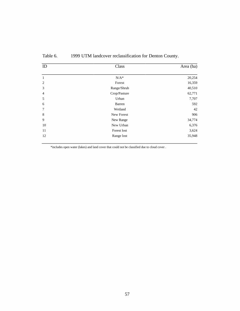
57

Table 6. 1999 UTM landcover reclassification for Denton County.

*includes open water (lakes) and land cover that could not be classified due to cloud cover .

ID Class Area (ha) 1 N/A* 20,2542 Forest 16,3593 Range/Shrub 40,5104 Crop/Pasture 62,7715 Urban 7,7076 Barren 5927 Wetland 428 New Forest 9069 New Range 34,77410 New Urban 6,37611 Forest lost 3,62412 Range lost 35,948

58

Table 7. Patch metrics – Edge. NUMBP TE ED MPE Site # of patches total edge edge density mean edge/ patch meters meters/hectare meters 1 34 57,238.98 0.24662 1,684.9247 2 33 29,010.49 0.12500 1,834.8775 3 49 81,368.39 0.35059 1,771.0323 4 46 69,520.91 0.29954 1,521.9670 5 28 50,262.36 0.21656 1,889.2525 6 32 67,466.25 0.29069 2,180.9950 7 35 66,086.26 0.28474 1,902.5320 8 37 68,202.25 0.29386 1,865.6460 9 50 72,725.55 0.31335 1,539.3852 10 53 72,219.56 0.31117 1,388.5255 11 46 76,804.20 0.33092 1,685.5052 12 46 73,538.25 0.31685 1,794.9140 13 46 62,212.06 0.26805 1,376.0393 14 42 72,188.88 0.31104 1,716.7430 15 41 77,218.19 0.33271 1,883.3710 16 44 79,824.84 0.34394 1,814.2235 17 43 74,994.87 0.32313 1,806.2210 18 42 67,650.25 0.29148 1,645.7470

59

Table 8. Landscape metrics – Fragmentation and Interspersion. NUMBP (number of patches). TE (total edge) TE = sum of perimeter in meters. ED (edge density) ED = TE / landscape area. LSI (landscape shape index) LSI >/= 1 without limit. MSI (mean shape index) MSI >/= 1. IJI (interspersion juxtoposition index) 0 >IJI < 100. Site NUMBP TE ED LSI MSI IJI Forest 4022 65.70 2895791.61 39.68 1.71 44.80 Rangeland/Shrubland 8724 240.50 10602340.08 130.73 1.95 59.50 Pasture/Cropland 7430 215.70 9509828.48 118.50 1.84 53.03 Urban 4384 50.40 2221035.79 32.29 1.66 75.27 Barren 7635 57.20 2523726.35 34.76 1.67 69.66 Wetland 31 0.30 11793.45 6.51 1.66 43.63

60

Table 9. Habitat metrics per research site - water. Strmden = stream density, shrlnden = shoreline density, dtrip = distance to riparian zone in four cardinal directions: north,east,south, and west. In absence of stream, L = lake shoreline. N/A = nearest stream is beyond County boundary. metric strmden shrlnden dtripn dtripe dtrips dtripw m/2.6 km2 m/2.6 km2 km km km km site (m/mi2) (m/mi2) 1 0.00 8,862.72 L0.96 L0.61 L1.08 L1.54 2 0.00 4,818.79 N/A L0.56 L0.85 L1.19 3 3,753.76 0.00 0.00 0.21 0.40 0.69 4 3,156.52 1,003.72 0.00 0.03 2.27 0.05 5 2,339.12 0.00 0.00 0.45 1.22 N/A 6 7,473.84 0.00 0.05 0.03 0.05 0.06 7 3,950.39 411.71 0.00 0.35 1.60 1.01 8 5,285.49 0.00 0.13 0.23 1.22 2.29 9 3,205.57 0.00 2.35 0.26 0.93 1.29 10 6,125.70 599.17 0.10 0.11 0.14 2.09 11 2,801.34 495.90 0.47 0.43 0.98 0.72 12 2,828.65 499.36 1.54 1.13 0.27 2.01 13 1,962.03 8,819.48 0.50 0.61 0.47 L0.80 14 4,534.59 0.00 0.56 0.06 0.27 0.77 15 685.58 10,493.67 L0.61 L1.01 0.43 0.98 16 4,095.03 0.00 0.66 1.82 L1.53 L0.71 17 4,853.97 0.00 0.35 0.35 0.63 1.26 18 4,889.96 0.00 2.35 0.43 0.13 0.21

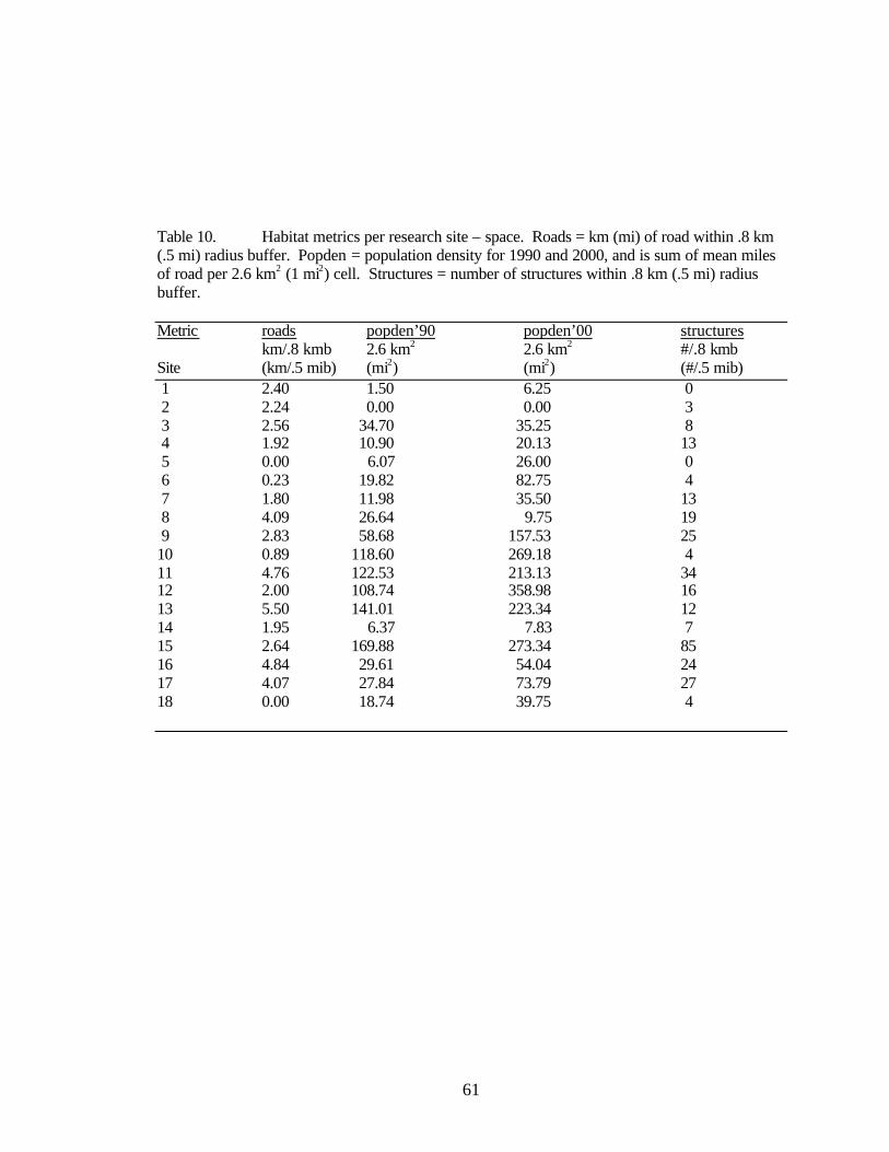
61

Table 10. Habitat metrics per research site – space. Roads = km (mi) of road within .8 km (.5 mi) radius buffer. Popden = population density for 1990 and 2000, and is sum of mean miles of road per 2.6 km2 (1 mi2) cell. Structures = number of structures within .8 km (.5 mi) radius buffer. Metric roads popden’90 popden’00 structures km/.8 kmb 2.6 km2 2.6 km2 #/.8 kmb Site (km/.5 mib) (mi2) (mi2) (#/.5 mib) 1 2.40 1.50 6.25 0 2 2.24 0.00 0.00 3 3 2.56 34.70 35.25 8 4 1.92 10.90 20.13 13 5 0.00 6.07 26.00 0 6 0.23 19.82 82.75 4 7 1.80 11.98 35.50 13 8 4.09 26.64 9.75 19 9 2.83 58.68 157.53 25 10 0.89 118.60 269.18 4 11 4.76 122.53 213.13 34 12 2.00 108.74 358.98 16 13 5.50 141.01 223.34 12 14 1.95 6.37 7.83 7 15 2.64 169.88 273.34 85 16 4.84 29.61 54.04 24 17 4.07 27.84 73.79 27 18 0.00 18.74 39.75 4

62

Table 11. Number of white-tailed deer per research site and different census method. Research Site 1 2 3 4 5 6 7 8 9 10 11 12 13 14 15 16 17 18 Census Owner Impression* 15 n/r 25 10 n/r 8 11 11 12 20 5 7 0 n/r n/r 50 12 20 Spotlight Census** 0 3 0 0 5 0 0 0 0 0 0 0 0 0 0 0 0 0 Camera Census*** 25 15 9 0 21 9 6 5 4 17 0 0 0 5 0 0 0 4 * represents owner’s estimates of deer on property ** represents deer observed during three mile spotlight census performed Mar. & Apr. 2002. *** represents deer photographed in Aug. 2001 and Jan. 2002.

Table 12. White-tailed deer sign per research site. X = presence of sign. Research Site Sign 1 2 3 4 5 6 7 8 9 10 11 12 13 14 15 16 17 18 Tracks X X X O X X X X X X X X O X O X X X Droppings X X X O X X X X O X X X O X O X X X Rubs/Scrapes O X O O X X O O O O O X O O O O X X Antlers O O O O O O O O O O O O O O O O X O

63

Figure 13. 18 research sites with .8 km (.5 mi) radius buffers. (1 mi = 1.6 km).

#

#

#

#

#

#

##

#

#

#

#

#

#

#

#

#

#

Site 3, Bolivar

Site 1, Isle du Bois

Site 2, Johnson Branch

Site 4, Krum

Site 5, Stony

Site 6, Drop

Site 7, UNTWRS Site 8, Denton west

Site 9, Flower Mound

Site 10, Roanoke

Site 11, Copper Canyon

Site 12, Lewisville

Site 13, Little Elm

Site 14, NavoSite 15, Denton east

Site 16, Crossroads

Site 17, Aubrey

Site18, Pilot Point

10 0 10 Miles

Denton County Boundary.5 Mile Radius Buffer

# Research Site

N

EW

S

Denton County

64

Figure 14. 1988 Landcover. Produced from Landsat Thematic Mapper (TM) Satellite images with a spatial resolution of 30 m x 30 m. (1 mi = 1.6 km).

#

#

#

#

#

#

##

#

#

#

#

#

#

#

##

#

10 0 10 Miles

1988 Landcover ReclassificationForestRangeland/ShrublandPasture/CroplandUrbanBarrenWetlandNo Data

# Research Sites

N

EW

S

65

Figure 15. 1999 Landcover. Produced from Landsat Thematic Mapper (TM) Satellite images with a spatial resolution of 30 m x 30 m. (1 mi = 1.6 km).

#

#

#

#

#

#

##

#

#

#

#

#

#

#

##

#

10 0 10 Miles

1999 Landcover ReclassificationForestRangeland/ShrublandPasture/CroplandUrbanBarrenWetlandNo Data

# Research Sites

N

EW

S

66

Figure 16. Change in Landcover from 1988 – 1999. Produced from Landsat Thematic Mapper (TM) Satellite images with a spatial resolution of 30 m x 30 m. (1 mi = 1.6 km).

#

#

#

#

#

#

##

#

#

#

#

#

#

#

##

#

10 0 10 Miles

Landcover Change from 1988 - 1999N/AForestRange/ShrublandCrop/Pasture landUrban landBarren landWetlandNew ForestNew Range/ShrublandNew UrbanForest lostRange/Shrubland lostNo Data

# Research Sites

N

EW

S

67

Figure 17. Stream Density. Data set was acquired from the Texas Department of Transportation Urban Files for Fall 1999. The unit of measure is linear length in meters per 1-mile cell. (1 mi = 1.6 km).

#

#

#

#

#

#

##

#

#

#

#

#

#

#

##

#

10 0 10 Miles

Stream Densi ty21 - 837837 - 16171617 - 22512251 - 28922892 - 35993599 - 43614361 - 53655365 - 67686768 - 87068706 - 11816

# Research Sites

N

EW

S

68

Figure 18. Shoreline Density. Data set was acquired from the Texas Department of Transportation Urban Files for Fall 1999. The unit of measure is linear length in meters per 1-mile cell. (1 mi = 1.6 km).

#

#

#

#

#

#

##

#

#

#

#

#

#

#

##

#

10 0 10 Miles

Shoreline Density16 - 698698 - 13181318 - 18041804 - 24182418 - 39243924 - 53545354 - 70987098 - 92809280 - 1242012420 - 17799

# Research Sites

N

EW

S

69

Figure 19. 1990 Average Population Density. Population grid coverages were produced using census tract centroids with a search radius of 1 mile and with units in miles. The resulting grid coverages were intersected with the 1-mile cell grid and each cell’s corresponding density statistics were averaged. (1 mi = 1.6 km).

#

#

#

#

#

#

##

#

#

#

#

#

#

#

##

#

10 0 10 Miles

1990 Average P opulation 0 - 5757 - 15 3153 - 2 88288 - 4 64464 - 7 39739 - 1 1301130 - 17351735 - 24182418 - 34533453 - 4543

# Research S ites

N

EW

S

70

Figure 20. 2000 Average Population Density. Population grid coverages were produced using census tract centroids with a search radius of 1 mile and with units in miles. The resulting grid coverages were intersected with the 1-mile cell grid and each cell’s corresponding density statistics were averaged. (1 mi = 1.6 km).

#

#

#

#

#

#

##

#

#

#

#

#

#

#

##

#

10 0 10 Miles

2000 Average Popu lation0 - 7373 - 189189 - 361361 - 593593 - 880880 - 13721372 - 20002000 - 28562856 - 39043904 - 5651

# Research Sites

N

EW

S

71

Figure 21. Site 1, Isle du Bois, DOQQ showing research site and .5 mile radius buffer. (1 mi = 1.6 km).

#

72

Figure 22. Site 3, Bolivar, DOQQ showing research site and .5 mile radius buffer. (1 mi = 1.6 km).

#

73

Figure 23. Site 5. Stony, DOQQ showing research site and .5 mile radius buffer. (1 mi = 1.6 km).

74

Figure 24. Site 9, Flower Mound, DOQQ showing research site and .5 mile radius buffer. (1 mi = 1.6 km).

#

75

Figure 25. Site 14, Navo, DOQQ showing research site and .5 mile radius buffer. (1 mi = 1.6 km).

#

76

CHAPTER 4

RESULTS & DISCUSSION

The majority of the 18 research sites were located in Alfisol and Entisol soil orders

(Table 4), and Upper Cretaceous and Recent Geologic Formations (Table 3). Sites 1, 2, 9,

and 13-17 were in Alfisols, which closely correspond with the Woodbine Formation. The

Woodbine Formation closely matches up with the Eastern Cross Timbers Physiographic

Region, with Post Oak (Quercus stellata), Blackjack Oak (Quercus marilandica), Greenbriar

(Smilax bona-nox), and Poison Oak (Toxicodendron radicans). The Recent Series is

alluvium along the flood plains, is the parent material for sandy loam Entisol, and is the

location for sites 5-7, 10, 11, and 18. These sites were in riparian zones and contain Pecan

(Carya illnoensis), Cottonwood (Populus deltoids), Greenbriar (Smilax bona-nox), and

Poison Oak (Toxicodendron radicans).

At the landscape level Denton County has experienced several changes in landcover

from 1988 to 1999 (Table 5). Table 6 reveals 163,589,200 m2 of forest, 405,095,136 m2 of

rangeland /shrubland, 627,705,920 m2 of cropland/pasture, 77,070,336 m2 of urban land,

5,924,726 m2 of barren land, and 423,195 m2 of wetland. There were 9,064,831 m2 of new

forest, 347,740,032 m2 of new rangeland/shrubland, 63,763,216 m2 of new urban land,

36,241,456 m2 of forest lost, and 359,479,456 m2 of rangeland/shrubland lost. The

202,538,160 m2 labeled N/A includes both open water and landcover that could not be

77

classified due to possible cloud cover.

According to the United States Army Corp of Engineers (2002), there were two

important changes, regarding lakes in Denton County, between 1988 and 1999. First, Lake

Ray Roberts reached its ultimate surface level. This resulted in a large portion of habitat

being inundated, but this also transformed many of acres of surrounding cropland into

rangeland/shrubland. Second, the level of Lake Lewisville was raised 2.13 m (7 ft), causing

another reduction in forest and rangeland/shrubland. What data in Table 6 does not reveal is

that, except for two areas in the southwest portion of the county including Texas Motor

Speedway and Alliance Airport, nearly all of the increase in urban classification seems to

have taken place within the perimeters of existing urban areas and not in areas where high

densities of white-tailed deer would be expected. Nearly all of the forest lost was in

individual large tracts, and except in a couple of areas in the eastern part of the county where

forest lost was probably due to strip mining of sand and gravel, nearly all took place in three

developments. Two of the developments are in Flower Mound and one is in Highland

Village (Figure 16).

Denton is in the center of the county, and the majority of the urban areas are in the

southeast quadrant, which leaves approximately three-fourths of the county rural. Table 6

shows that over 35,900 ha of rangeland/shrubland was lost and 34,700 ha of

rangeland/shrubland was gained from 1988 to 1999. Generally, a large percentage of the

rangeland/shrubland lost was in the southeast quadrant, where the patches were fragmented.

This fragmentation came about because of extensive urbanization and the way the growth in

development and population has increased in relation to Lake Lewisville. Although there are

78

isolated pockets of white-tailed deer in this quadrant, expectations for herd sustainability

would have to be low in most cases. One exception to this would be the area below the Lake

Lewisville dam, which is regulated by the United States Army Corp of Engineers. If the

landcover data in this quadrant could be deducted from the total, the remainder of the county

should show an increase in habitat, such as rangeland/shrubland for example. Based on

habitat, white-tailed deer sustainability in the northern and western three-fourths of the

county is quite possible. Also, note that a good portion of the unclassified image in 1999 was

rangeland/shrubland and forest in 1988. This is especially evident in the area of the Wildlife

Management Area, north of Lake Lewisville and along the Elm Fork of the Trinity River

(Figure 16).

It is difficult to evaluate which site had the best food and cover in that white-tailed

deer are so adaptable and eat such a variety of browse, forbes, and grasses. Sites located in

the Cross Timbers had suitable natural vegetation (Post Oaks) for cover and food, although

the sites in riparian areas, when adjacent to agricultural crops and/or woodlots were probably

the best over all. Sites 3, 5, 6, 8, and 14 are all located along a stream with native vegetation

and also have fields of wheat and grain sorghum (Table 2). Photographs of white-tailed deer

were produced at all five of the above sites, with Site 5 producing the most. Site 5 was also

one of the sites in which deer were observed during the spotlight census.

Regarding patch metrics (Table 7) total edge (TE), edge density (ED), and mean edge

per patch (MPE), sites 15, 3, 16, 11, and 17 exceeded those of the others. Of the above sites,

only Site 3 produced photographs of white-tailed deer. Water is seldom a determining factor

in habitat, and this is especially true for Denton County, because of the many streams, lakes,

79

stock tanks, and springs. Site 6 ranked highest (Table 9) in both stream density (strmden)

and distance to riparian in all four cardinal directions (dtrip). Site 15 ranked highest in

shoreline density (shrlnden). Of the two sites only Site 6 revealed the presence of white-

tailed deer in photographs. Sites 1, 5, 2, and 6 ranked highest in roads, population density

(popden), and structures (Table 10). White-tailed deer were photographed at all sites, and

Site 1 produced the highest amount of any in the county. Site 2 was the only other site where

deer were observed during the spotlight census.

With respect to patch metrics, it appears that Sites 3, 5, and 6 have the highest scores.

All three of them have both natural food and cover along major riparian zones, but also have

nearby fields of wheat and grain sorghum. Sites 5 and 6 scored high in space metrics –

population, roads, and struc tures. Five white-tailed deer were counted during the spotlight

survey at Site 5, and all three sites produced photographs during both periods of camera

census. Of the three, Site 5 produced more than the other two together. All three of the sites

were in the western half of the county, and all are in areas of habitat growth.

The relationships between number of white-tailed deer photographed and patch,

water, and space metrics were examined. Six of the 14 metrics had significant, but inverse,

Spearman rank correlation coefficients. The metrics were total edge (TE) at –0.552, edge

density (ED) at-0.552, roads at –0.539, 1990 population density (popden’90) at –0.575, 2000

population density (popden’00) at –0.516, and number of structures at –0.811 at a 95%

significance level. The study illustrates that of the indices or metrics structures had the

strongest Spearman rank correlation coefficients. Total edge (TE) and edge density (ED)

were somewhat surprising in that one would assume a site with a greater amount of edge

80

would be better habitat and produce a greater number of photographs. However the opposite

was true. This could be because of poor site location or the fact that white-tailed deer are not

as attracted to bait in areas of better habitat. The 2000 population density (popden’00) at –

0.516 was not as significant as the 1990 population density (popden’90) at –0.575. This

could be because the numbers of white-tailed deer are increasing despite a growth in the

human population. The Spearman correlation coefficients that were not significantly

correlated was number of patches (NUMBP) at –0.434, mean edge per patch (MPE) at 0.201,

stream density (strmden) at 0.035, shorline density at (shrlnden) at –0.072, distance to

riparian north (dtripn) at –0.327, distance to riparian east (dtripe) at –0.264, distance to

riparian south (dtrips) at –0.084, and distance to riparian west (dtripw) at 0.249.

When asked how many white-tailed deer are in the area of their property, the

responses from landowners/agents covered a wide range (Table 11). The extremes are sites

13 and 16. The landowner at Site 13 did not believe there are white-tailed deer in his area,

while the landowner at Site 16 believed the number to be in excess of 50. Actually, even

though the two sites are a few miles apart, both are probably fairly accurate in their estimates.

The landowner at Site 13 has not observed any deer, none were photographed during the

camera census, and the area is mostly residential with a high population density and a high

number of structures. Despite these facts, it is highly possible that some white-tailed deer are

in the fringes of this area, and are nocturnal in their movements. There is a great deal of

open land that is overgrown in mesquite and juniper, and as Table 9 illustrates, the shoreline

of Lake Lewisville is not greater than .63 miles away in any of the four cardinal directions.

Site 16 is an area of rugged hills covered in Post Oak. Even though it has some

81

commercial development occurring and a busy highway running through it, the white-tailed

deer numbers are great enough that the landowner felt the necessity to manage the deer by

hunting. Site 16 was adjacent to the Wildlife Management Area on the north end of Lake

Lewisville and a number near fifty is possible. These responses are not too dissimilar from

general reactions around the county. Some people were not aware of any white-tailed deer

being in Denton County, or the entire area, while some said they had been observing them on

a regular basis for the last 10 years or so.

As stated above, the spotlight census was not very successful in that white-tailed deer

were observed at only two of the sites (Table 11). At earlier times, deer were observed by

spotlight at some of the sites. At Site 1, no deer were seen during this census, but a couple of

months earlier in another research project, 25 or more were observed. Site 12 revealed no

deer during the census but often when checking the camera, deer would be seen in the fields

and along the road.

Antlered white-tailed deer (bucks) were easy to identify during both camera census

periods, as were antlerless (does and fawns) in August (Table 11). Antlerless white-tailed

deer were difficult to identify, and subsequently quantify, in January as fawns were about the

size of some of the mothers, and the young bucks had not began antler growth. The

photographs revealed some interesting phenomena. No deer were photographed in August at

Site 1, but over-all this site had the greatest total number of deer with 25 being photographed

in January. Site 5 revealed only antlered (bucks) in August and both antlered and antler- less

in January. The majority of the bucks photographed in January did not appear to be the same

ones that were present in August. Only antler- less white-tailed deer (does and fawns) were

82

present at Site 10, in August but January photographs revealed deer of both sexes. Other

deer at Site 10 exhibited similar scarring across their backs. Site 18 had no photographs of

white-tailed deer in August, but in January four deer were photographed. The antlers on

certain bucks at Site 1 and some at Site 2 showed malformations such as palmation, split

brow tines, drop tines, and kickers. Sites 1 and 2 are adjacent to the Trinity River drainage

area and the Lake Ray Roberts Greenbelt, where another research is in progress. The

investigator in that 2-year study is researching the movement of white-tailed deer in a

corridor. An estimate of the number of deer present along the Greenbelt and adjoining

Wildlife Management Area is 45, and many of the bucks exhibit the same antler

characteristics as those photographed at Sites 1 and 2.

At Site 1, Isle du Bois, no white-tailed deer were observed and/or photographed in

August, but the January census revealed 13 antlered and 12 without antlers, for a total of 25.

Apparently, in August, the deer did not find the bait pile until after the census period. Two

days after removal of camera, three deer were observed eating at the site. At Site 2, Johnson

Branch, nine antlerless and six bucks were photographed during the two census periods.

Photographs from this site revealed the presence of a mature 12-point buck in January. This

buck is a typical eight but has a split brow tine, forked G-2s, and a drop tine. Site 3, Bolivar,

generated photographs of two antlered and seven antlerless white-tailed deer, although more

were observed at the site. Site 4, Krum, produced no photographs. At Site 5, Stony, 21

white-tailed deer were photographed, 16 with antlers and five without. This site had several

young bucks, especially one eight point with an inside spread that appeared to exceed 51 cm

(20 in). Site 6, Drop, generated photographs of nine deer, of which three were males and six

83

were antlerless. At Site 7, Water Research Station, six white-tailed deer were photographed

in August but none in January. There were two young bucks, three does, and one fawn. At

Site 8, Denton West, five deer were photographed, one a young buck and the rest does. At

Site 4, Flower Mound, four antler-less white-tailed deer were photographed in January but

none in August. Seventeen white-tailed deer were photographed at Site 10, Roanoke,

including five bucks and 12 without antlers. Site 11, Copper Canyon, produced no

photographs, although property owners reported observing white-tailed deer feeding on pears

during August. Site 12, Lewisville, also produced no pictures but white-tailed deer were

observed in the area. Site 13, Little Elm, produced no pictures. Site 14, Navo, revealed five

antler- less white-tailed deer. Site 15, Denton East, generated no pictures. Site 16, Cross

Roads, produced no pictures as the camera was stolen within a couple of days of setting it.

Site 17, Aubrey, also produced no pictures, although a great deal of “sign” was present at

both the Cross Roads and Aubrey sites (Table 12). Site 18, Pilot Point, had pictures of one

buck and three doe, for a total of four in January.

Although steps were taken to avoid photographing non-target animals, many rolls of

film were spent on various wildlife, birds, feral hogs (Sus scrofa), and others. The various

wildlife included Raccoon (Procyon lotor), Eastern Cottontail Rabbit (Sylvilagus floridanus),

Striped Skunk (Mephitis mephitis), Coyote (Canis latrans), and Eastern Fox Squirrel

(Sciurus niger). Birds included, but were not limited to, wild turkey (Meleagris gallopavo,

mourning dove (Zenaida macroura), blue jay (Cyanocitta cristata), and one emu

(Struthioniform). Site 18 was the only one to produce photographs of feral hogs, although

signs of this species were observed at others. There were approximately 50 different feral

84

hogs photographed at Site 18. In addition to the above animals, there were photographs of

burros (Equus asinus), dogs (Canis familiaris), and people on foot, on horseback, and in

motor vehicles.

85

CHAPTER 5

CONCLUSIONS

If one looks at just the data in Table 6, it would appear that there has in fact

been a decrease in white-tailed deer habitat since 1988. However when looking at the

coverages in Figures 14, 15, and 16, it is apparent that much of the reduction in

rangeland/shrubland and forest occurred: 1) because of an increase in lake levels, 2)

because of urban growth within the limits of existing cities, 3) in the southeast one-

fourth of the county, and 4) because of the unclassified data in the area north of Lake

Lewisville and other locations.

According to the United States Army Corp of Engineers (2002), the level of

Lake Lewisville was raised from 157 m (515 ft) above mean sea level to 159 m (522

ft) in November 1988, and Lake Ray Roberts rose to the final level of 193 m (632 ft)

in March 1990. Habitat was obviously lost with the completion of these two projects.

It is difficult to know exactly how much habitat was inundated by the increase in lake

levels, but it is possible that the change in levels was not all negative with regards to

white-tailed deer habitat. Much of the property in the area of Lake Ray Roberts was

cropland/pasture and is now rangeland/shrubland.

The major cities of Denton County including Denton, Lewisville, Carrollton,

and The Colony do not appear to have increased their city boundaries but have filled

86

fragmented, undeveloped areas within their established boundaries (Figures 14, 15,

and 16). The exceptions are Lewisville that has expanded eastward along Highway

121 and Carrollton that has expanded northward towards Lewisville. Some of the

smaller communities such as Corinth, Lake Dallas, Little Elm, and Roanoke have also

experienced an increased amount of development.

A large percentage of the forest and range land/shrubland lost was in the

southeast quadrant where the patches were fragmented. This fragmentation came

about because of extensive urbanization and the way the growth in development and

population has increased in relation to Lake Lewisville. This area is mostly urban

and has experienced some of the highest population growth rates, while the remainder

is still used for farming but is not very conducive to white-tailed deer. The

rangeland/shrubland and forest that was lost in this area was not white-tailed deer

habitat.

A significant amount of forest and rangeland/shrubland in Figure 8 is

classified as N/A in Figure 16. This is especially apparent in the riparian zones

throughout the county. A large portion of the Elm Fork of the Trinity River and the

Wildlife Management Area north of Lake Lewisville is shown as forest and

rangeland/shrubland in Figure 14, but unclassified in Figure 16. It is similar for the

remaining streams in the Lake Lewisville watershed area. These include, but are not

limited to Clear Creek, all three Hickory Creeks, Little Elm Creek, and Stewart

Creek. The same is also true with all of the streams in the Denton Creek drainage

system and Lake Grapevine. Many patches of unclassified data appear in the

87

westernmost edge of the Cross Timbers where they were classified as forest and

rangeland/shrubland in 1988.

In the northern and western three quadrants of the county, habitat has

increased, because 1) large monoculture farms and ranches are being broken up into

smaller parcels, creating a patchwork, 2) many of these parcels are either fallow or

they are non- improved pasture of tenant ranchers, 3) more farmers and ranchers are

planting native hay, 4) many of the parcels that are developed become multi-acre

ranchettes where the bulk is allowed to grow and only a small area around the

residence is improved, 5) many of the parcels are providing connectivity between

exiting woodlots, riparian zones, and planted fields, and 6) a large percentage of the

people in this county are willing to make an effort to ensure that white-tailed deer

remain here. In all the interviews I performed, only one person said they did not want

them on their property and that was because a fear that they might spread disease to

her horses.

Even from the major roadways, it is apparent that the improved fields are both

fewer and smaller in Denton County. Interstate 35W, Highway 380, FM 455, and FM

156, are but a few of the roads where this is evident. This increase in habitat is

possibly responsible for an increase in white-tailed deer sightings from vehicles. This

could be because of an increase in quantity but also because the white-tailed deer are

more visible, in that they are no longer confined to the creek bottoms as they once

were.

Geographic Information Systems and Remote Sensing are effective tools

88

in habitat evaluation. Rather than just looking at data, as beneficial as that is, GIS

presents a very real image for the viewer, and the addition of aerial and satellite

imagery enhances the capabilities of GIS. In this research infrared-triggered cameras

proved superior to both spotlight census and owner’s impressions. Land owners’

impressions, while offering good information, are arbitrary at best as a census tool.

There are too many outside factors that could influence them. Land owners’

impressions could be more reliable in the Hill Country or South Texas where they

have been observing white-tailed deer for their entire lifetime. If the spotlight census

had been performed multiple times along the same routes, it is possible it could have

provided more accurate data as to the quantity and quality of white-tailed deer in the

area. Although I tried to remain objective, I cannot say that I did not have some

expectations. Some sites that I thought would produce pictures did not. Site 11 was

located approximately 100 meters east of a residence and did not photograph any

white-tailed deer but they were observed eating pears forty meters west of the

residence. This site is on the fringe of a very large bottomland forest in the Hickory

Creek drainage basin and should have a high number of deer even though it is quite

populated. Site 17 produced no photographs despite appearing to be as likely a

location as one could expect. It consists of very steep hills covered in Post Oak and

Greenbrier. There is no hunting allowed anywhere near the property and it is

adjacent to the Wildlife Management Area. White-tailed deer are present because

numerous tracks, droppings, rubs, and one pair of shed antlers were found. Often

white-tailed deer photographed does not equate to habitat quality. In order for the

89

cameras to work the deer have to be baited to the site. When habitat quality is high

they may not be attracted to bait, so sometimes more marginal habitat may produce

more photographs. Another reason more sites weren’t successful is probably due

more to poor site location than anything else. Site 12 is a good example of this. This

property, located below the dam at lake Lewisville, is several hundred acres of

protected hardwood bottomland forest and rangeland/shrubland. I relied on someone

knowledgeable in the area to advise me on site location and now realize a better

choice may have been to do more scouting and choose the site for myself. The one

that was most surprising was Site 14 (Figure 5). I had no idea there were any white-

tailed deer that far south and east, in Denton County. Biologists from the Texas Parks

and Wildlife Department do not believe there to be a sufficient number of white-

tailed deer to justify a hunting season or even a spotlight census for Collin, Dallas,

and Rockwall Counties (Young and Traweek 2000).

The photographs not only revealed a conservative estimate of how many

white-tailed deer were in the area of each research site, but also conveyed the overall

health of the animals. Only one picture, last August, included a doe with ribs

showing. The norm was very healthy does with twin fawns and bucks of all ages.

Second, it was very evident that white-tailed deer spend different seasons in different

areas. I believe they keep to their one-mile +/- home range, but are often in different

areas in spring, summer, fall, and winter. This was especially evident at Sites 5 and

10. In August, photographs revealed only bucks at Site 5. January photographs

revealed both bucks and does, and the bucks were not the same as the ones in August.

90

In August, photographs revealed only does and fawns at Site 10, but in January, there

were bucks and does. Lastly, there seems to be a substantial number of varmints and

especially raccoons, which could result in potential health issues. Out of eleven rolls

of 24-exposure film I developed last January, I rejected 85 photographs that had only

raccoons, and that was only part of the total.

Habitat of white-tailed deer in Denton County and North-central Texas has

not been studied extensively. Although there has been extensive studies elsewhere

and at both the patch and landscape levels, none have been published regarding

white-tailed deer in limited habitat on as large a scale as Denton County. Perhaps this

research will inspire others to perform future studies so that white-tailed deer are here

to stay. Future research should attempt to determine the genetic source of white-

tailed deer in Denton County. When performing the Soil Survey of Denton County,

Ed Pauls recalls two tracks in Clear Creek, northwest of Bolivar. Did the white-tailed

deer of Denton County start there and expand east and south across the county, or did

they move in from Wise County in the west, or did they move south from Cooke and

Grayson County and the Red River basin? Any or all of the above is possible.

91

APPENDIX A

WAIVER OF CONSENT

92

Appendix A. Informed Consent Waiver & Release University of North Texas Special Projects Informed Consent Waiver & Release 1. In consideration for receiving permission to participate in the special problems

research project, Distribution of White-Tailed Deer in Denton County of North-Central Texas, known as Biology 4900.713 (“Activity”), I hereby release, waive, discharge and covenant not to sue the University of North Texas, the Board of Regents of the State of Texas, their officer, servants, agents, or employees, (“UNT”) and David Sallee, individually and officially from any and all liability, claims, demands, actions and causes of action whatsoever arising our of or related to any loss, damage, injury, including death, that may be sustained by me, or to any property belonging to me, whether caused by the negligence of UNT, or David Sallee, or otherwise, while participating in Activity or in transportation to and from Activity.

2. Voluntary Participation/Informed Consent

(a) To the best of my knowledge, I can fully participate in Activity. I am fully aware of the risks and hazards connected with the activity including, but not limited to, the risks as noted herein, and I hereby elect to voluntarily participate in Activity, and to engage in Activity knowing that Activity may be hazardous to me and my property. I voluntarily assume full responsibility for any risks of loss, property damage, illness or personal injury, including death, that may be sustained by me, or any loss or damage to property owned by me, as a result of being engaged in Activity, whether caused by the negligence of UNT or David Sallee, or otherwise.

(b) I am fully aware of and voluntarily assume full responsibility for any

risks involved in participation in Activity, such as the presence of harsh or unusual conditions, including, but not limited to, man-made hazards, commuting, transporting of supplies, site preparation, barriers, extreme heat, extreme cold, extended exposure to sun, wind, rain, rough or rocky terrain, animals, insects, vegetation, parasites, and bacteria.

• Man-made hazards includes but is not limited to daily activities of farm/ranch operations such as mowing, plowing, tending livestock, and oil/gas exploration, and hunting or discharging of firearms on site and/or adjacent properties.

93

Appendix A. cont.

• Commuting includes but is not limited to driving to and from research sites, riding as a passenger, parking, and ingress/egress from the vehicle.

• Transporting of supplies includes but is not limited to loading, transporting, and unloading of cameras, film, batteries, bait (corn), and any tools necessary to perform the task.

• Barriers include but are not limited to ditches, gullies, small streams, fences, barricades, and steep terrain.

• Animals include but are not limited to domestic livestock, dogs, white-tailed deer, feral hogs, coyotes, bob-cats, raccoons, skunks, opossums, and snakes.

• Insects include but are not limited to bees, wasps, hornets, ticks, chiggers, mosquitoes, spiders, ants, flies, and grasshoppers.

• Vegetation includes but is not limited to Mesquite, cactus, nettles, greenbriar, poison ivy, poison oak, poison sumac, bois d’arc and tall grasses and weeds.

3. I agree to indemnify and hold harmless UNT and David Sallee, individually

and officially from any loss, liability, damage or costs, including court costs and attorney’s fees, that may be incurred due to my participation in Activity, whether caused by negligence of UNT and/or David Sallee, or otherwise.

4. I understand that UNT and David Sallee will not be responsible for any

medical costs associated with any injury I may sustain while participating in Activity.

5. It is my express intent that this Informed Consent Waiver and Release shall bind

the members of my family and spouse (if any), if I am alive, and my heirs, assigns and personal representative, if I am not alive, shall be deemed as a release, waiver, discharge, covenant not to sue UNT and David Sallee. I agree that this Informed Consent Waiver and Release shall be construed in accordance with the laws of the State of Texas.

6. I agree to become familiar with the rules and regulations of UNT, and/or the

instructor leading this Activity, which concerns student conduct. I agree not to violate said rules or any directive or instruction made by the person or persons in charge of said program and that I will assume the complete risk of any activity done in violation of any rule or directive or instruction.

94

7. I understand that I should and am urged by UNT and David Sallee to obtain adequate health and accident insurance to cover any personal injury or property loss to myself that may be sustained during Activity or the transportation to and from Activity.

Appendix A. cont. In signing this release as a participant in August 2001 and January 2002 in a special problems research project, Distribution of White-Tailed Deer in Denton County of North-Central Texas, known as Biology 4900.713 (“Activity”), I certify that I have read the foregoing Informed Consent Waiver and Release, understand it and sign it voluntarily as my own free act and deed; no oral representations, statements or inducements, apart from the foregoing written agreement, have been made; I am at least eighteen (18) years of age and fully competent; or, if I am under eighteen (18) years of age, my parent or legal guardian’s approval and signature has been obtained; and I execute this Release for full, adequate, and complete consideration fully intending to be bound by the same. IN WITNESS WHEREOF, I have hereunto set my hand on this ______ day of ______________________, 20___. ____________________________________________ Participant’s signature (required) ____________________________________________ (witness) ____________________________________________ (witness)

95

APPENDIX B

LANDOWNER AGREEMENT

96

Appendix B. Landowners/Agents Consent

Landowner’s/Agents Consent to Participate in Research

Title of Research Project: Distribution of White-tailed Deer in Denton County of North-Central Texas Description: The purpose of this research is to estimate the quantity and location of white-tailed deer in Denton County. This will be achieved by conducting a point census at 18 locations distributed throughout the county and monitored by infrared-triggered cameras. The studies will take place in August 2001 and January 2002. Benefits: Having census data to work from is beneficial to Denton County residents because co-habitating with white-tailed deer offers aesthetic and recreational benefits as well as health and safety issues. University student-volunteers will learn white-tailed deer characteristics and behaviors as well as field research methods. Confidentiality: Confidentiality is very important to me. Although a map will illustrate the locations of my research sites, no names or addresses will be revealed. Voluntary Consent: I certify that I have read the preceding information and that I understand its content. I understand that no hunting will take place on the property during August 2001 and January 2002. I further understand that student-volunteers may assist in data collection. David Sallee has answered any questions I have about the research, and I grant David Sallee and/or his student-volunteers access to my property, known as ___________________________________, in the course of performing research in fulfillment of his degree at the University of North Texas. I understand that by granting access to my property, I become an active participant in the research and a friend of the University of North Texas.

97

__________________________________

Signature of Landowner and/or Agent/Date I certify that I have explained the nature and purpose of the research, have answered any questions, and have witnessed the above signature. Investigator: David Sallee, Graduate Student Department of Geography P.O. Box 305279 Denton, TX 76203-5279 940-565-2091

________________________________ Signature of Investigator/Date

98

APPENDIX C

LANDOWNER QUESTIONNAIRE

99

Appendix C. Landowner/Agent Questionnaire

White-Tailed Deer In Denton County Questionnaire

The study area consists of a ½ mile radius buffer illustrated by a circle on the aerial

photograph. Please study the photograph and answer the following questions that apply,

to the best of your knowledge. If a particular question does not apply, please respond by

placing N/A in the space provided.

1. How long have you lived, or managed property, in the area?

2. Do you believe white-tailed deer are present in the study area?

3. If you answered yes to question 2, how many white-tailed deer, in your

opinion, are there?

4. Have you seen white-tailed deer within the area defined by the ½ mile radius

buffer?

5. Have you observed “sign” within the area defined by the ½ mile radius buffer? “Sign” could be tracks, fecal pellet droppings, rubs, scrapes, and/or antler sheds.

6. Do you perceive the quantity of white-tailed deer to have increased, or decreased, in the time you have lived, or managed property, in the area?

7. In your opinion, what is the reason for the increase or decrease?

100

8. Do you believe the presence of white-tailed deer in Denton County is

beneficial or detrimental?

9. Why do you believe this?

10. If the presence of white-tailed deer is a benefit, what do you believe should be done to insure their presence for future generations?

_________________________________ ________________________________

David R. Sallee Landowner/agent

101

REFERENCE LIST

Anonymous. 1945. Principal Game Birds And Mammals Of Texas. Texas Game,

Fish and Oyster Commission. Von-Boeckmann-Jones Co. Austin, TX. Anonymous. Managing Riparian Habitats for Wildlife. Texas Parks and Wildlife

Department. PWD BR W7000-306 (6/98). Anonymous. 1999. Getting To Know ArcView GIS. Redlands, California:

Environmental Systems Research Institute, Inc. Anonymous. 1998. Riparian Forest Buffer. Natural Resources Conservation Service,

United States Department of Agriculture. 391. Baccus, J., R. Simpson, J. Dillard, and E.L.Young. 1998. Seasonal Food

Habits/Preferences of White-tailed Deer in the Cross Timbers and Prairies Region of North Texas. Wildlife Research Highlights, Vol. 3. Texas Parks and Wildlife Department.

Barnes, V. E. 1988. Geologic Atlas of Texas Dallas Sheet, Bureau of Economic Geology.

Bauer, E. 1993. Whitetails Behavior-Ecology-Conservation. Stillwater, MN:

Voyageur Press, Inc.

Bowman, J.L., M. Chamberlain, B.D. Leopold, and H.A. Jacobson. 1996. An evaluation of two censusing techniques to estimate black bear population size on White River National Wildlife Refuge, Arkansas. Proceedings of the Annual Conference of Southeast Association of Fish and Wildlife Agencies 50:386-390.

Brady, N., Weil, R. 1999. The Nature and Properties of Soils, Upper Saddle

River, New Jersey: Prentice Hall. Brothers, A., M. Ray. 1998. Producing Quality Whitetails, San Antonio, Texas:

Texas Wildlife Association.

102

Bryant, F.C., G. Van Vreede, T. Deliberto, and K. Gee. 1996. Diets of Female Whitetailed Deer in Cross Timbers Region. Prairie Naturalist. Vol. 28, No. 3: 125-140.

Clancy, G., L. Nelson. 1991. White-tailed Deer. Minnetonka, Minnesota: Cy

DeCosse Incorporated. Cobb, C.T., D. Francis, and R. Etters. 1993. Validating A Wild Turkey Population

Survey Using Cameras And Infrared Sensors. Congalton, R. and K. Green. 1992. The ABCs of GIS: an introduction to

geographic information systems. Journal of Forestry, November. Cooper, J. 1997. Native Plants To Use For Enhancing Wildlife Habitat. Denton

County, Texas Agricultural Extension Service Texas A&M University System.

Davis, W., D. Schmidly. 1994. The Mammals of Texas. Texas Parks and Wildlife

Department. Austin, Texas:University of Texas Press Demarais, S., W. McKinley, and H. Jacobson. 2000. Using Infrared-triggered

Cameras To Survey White-tailed Deer In Mississippi. Research Advances. Forest & Wildlife Research Center, Mississippi State University.

Dickson, K. L., D. Vance. 1981. Revegetating Sur face Mined Lands For Wildlife

In Texas And Oklahoma. Fish and Wildlife Service, U.S. Department of the Interior. FWS/OBS-81/25.

Dillard, J. 1994. Food Plots For White-tailed Deer In The Cross Timbers Region

Of North Texas. Texas Parks & Wildlife Department. Dillard, J. Herd Composition: An Essential Element of White-tailed Deer

Population and Harvest Management in the Cross Timbers of North Texas. Texas Parks and Wildlife Department Vol.5, No.2 (Summer 1996).

Dyksterhuis, E.J. 1946. The Vege tation Of The Fort Worth Prairie. Ecological

Monographs, 16: 1-28. Elkie, P., R. Rempel, and A. Carr. 1999. Patch Analyst. Center for Northern Forest

Ecosystem Research, Ontario Ministry of Natural Resources, Lake Head University, Thunder Bay, Ontario, Canada.

Ely, Melissa. 2002. United States Army Corp of Engineers. personal communication.

103

English, B. 2002. United States Department of Agriculture, Farm Service Agency. personal communication.

ESRI. 1998. ArcView GIS. Environmental Systems Research Institute, Redlands,

California, USA. Ford, A., E. Pauls. 1978. Soil Survey of Denton County Texas, United States

Department of Agriculture Soil Conservation Service. Frentress, C.D. 1986. Bottomland Hardwoods in Texas. Proceedings of an

Interagency Workshop on Status and Ecology. Texas Parks and Wildlife, U.S. Fish and Wildlife Service, Southern Forest Experiment Station, U.S. Forest Service.

Gee, K. 2000. A picture is worth a ? NF-Ag News and Views. Samuel Roberts

Noble Foundation. http:www.noble.org Gee, K., M. Porter, S. Demarais, F. Bryant, and G. Vreede. 1994. White-tailed

Deer: Their Foods And Management In The Cross Timbers, Ardmore, Oklahoma: Samuel Roberts Noble Foundation Publication.

Gregg, W.P. 1994. Developing Landscape-Scale Information to Meet Ecological,

Economic, and Social Needs. Remote Sensing and GIS in Ecosystem Management. Washington D.C.: Island Press.

Halls, L. K. 1984. White-tailed Deer Ecology and Management, Harrisburg,

Pennsylvania: Stackpole Books. Handley, M. December 1999. The Next Level of Deer Management.

Buckmasters. http:www.buckmasters.com Heffelfinger, J. 2000. Thoughts On Deer Density. Texas Trophy Hunters. January/February:116-118. Hellickson, M. 1999. Helicopter Census Techniques. South Texas Wildlife Caeser

Kleberg Wildlife Research Institute Vol. 3 No. 4.

Higganbotham, B. 2000. personal communication. Higganbotham, B., J. Kroll. 1992. Supplemental Forage Management for East Texas

White-tailed Deer. Texas Agricultural Extension Service.

Hood, R. 1998, November 8. Whitetail earns spot in history. The Fort Worth Star Telegram, p. D19.

104

Jacobson, Harry. 2000. Infra-red Camera Census of Whitetailed Deer. Whitetail

Times. XVI, 1:8-12. Kroll, J. C. and B. Koerth. 2000. Infrared Triggered Cameras: A Revolution in

Deer Management Technology. Texas Trophy Hunters. March/April:20-30.

Lambert, B. and T. Fullbright. 1998. Influence of Vegetation Diversity on White-tailed Deer Diets. Caesar Kleberg Wildlife Research Institute, Kingsville, TX.

Lyons, R. K., R. Machen, and T.D.A. Forbes. 1996. What Range Herbivores

Eat-and Why. Texas Agricultural Extension Service. B-6037. Lyons, R. K., R. Machen, and T.D.A. Forbes. 1995. Understanding Forage

Intake in Range Animals. Texas Agricultural Extension Service. L-5152. Lyons, R.K., T. Ginnet. 1998. Integrating deer, quail, and turkey habitat. Texas

Agricultural Extension Service. L-5196. Mace, R.D., S.C. Minta, T.L.Manley, and K.E. Aune. 1994. Estimating grizzly

bear population size using camera sightings. Wildlife Resources 21:657-666.

McGarigal, K., S. A. Cushman, M. C. Neel, and E. Ene. 2002. FRAGSTATS: Spatial Pattern Analysis Program for Categorical Maps. Computer softwareprogram produced by the authors at the University of Massachusetts, Amherst. Available at the following web site: www.umass.edu/landeco/research/fragstats/fragstats.html

McKnight, T.L., D. Hess. 2000. Physical Geography: A Landscape Appreciation. Upper Saddle River, New Jersey: Prentice Hall Publishing.

McMullin, S. 2000. Deer Program Supply and Demand, Virginia Department of

Game and Inland Fisheries, http:www.dgif.state.va.us. McNatt, M.R. 2001. personal communication. Miller, K.V., R.L. Marchinton. 1995. Quality Whitetails – The Why and How of

Quality Deer Management. Mechanicsburg, PA: Stackpole Books. Newell, J. 1996. A Landscape Ecological Characterization of the Ray Roberts

Lake Study Area, North-Central Texas: Temporal Variations in Landscape Pattern, 1987-1992. Master of Science Thesis, University of North Texas.

105

Nyerges, T. 1993. Understanding the Scope of GIS: Its Relationship to Environmental Modeling. Environmental Modeling With GIS. New York: Oxford University Press.

Pauls, E. 1999. personal communication. Phillips, K. 1999. Wildife Study Could Help Resolve State’s Fragmented Land

Issue. Ag News, Texas A&M University. Poteet, M., R. Thill, R.M. Whiting, and R. Lee Rayburn. 1996. Deer Use of

Riparian Zones and Adjacent Pine Plantations in Texas. Proceedings of the Annual Conference of the Southeast Association of Fish and Wildlife Agencies 50:541-549.

Rakestraw, D., N.J. Silvy. 1995. Comparison of Precision of Three Roadside

Counts for Estimating Deer Density. Wildlife Ecology and Management. Ramos M. G. (Ed). 1998. Texas Almanac, 1998-1999, Dallas, Texas: Dallas

Morning News, Inc. Rideout, D. The Post Oak Savannah Deer Herd Past, Present, Future. Texas

Agricultural Extension Service. PWD-RP-7100-193-4/91. Rollins, D. 1999. Fragmentation: A Dark Force in Wildlife Management.

http://texnat.tamu.edu/rollins. Rollins, D., J.D. Whipple, and W.A. Schacht. 1994. A Simple Technique For

Assessing Accuracy In Spotlight Deer Surveys. Texas Agricultural Extension Service. http://texnat.tamu.edu/rollins.

Rue, L. L. 1997. The Deer of North America, New York:Crown Publishers. Scoggins, P. 1999. Surface Geology of Dallas and Tarrant Counties, Texas,

Dallas Paleontological Society, http:www.dallaspaleo.org. Shult. M. J., Armstrong, B. 1999. Deer Census Techniques, Texas Agricultural

Extension Service, Texas Parks and Wildlife Department. Skipworth, S. 2000. personal communication. Smith, D. 1997. Remote Sensing of landscape- level Ecological Attributes at Ray

Roberts Lake in North Texas. Doctor of Philosophy, University of North Texas.

106

Spalinger, D., S. Cooper, D. Martin, and L. Shipley. 1997. Is Social Learning An Important Influence On Foraging Behavior In White-tailed Deer? Journal of Wildlife Management 61, (3), 611-621.

State Soil Geographic Data Base (STATSGO). 1993. United States Department

of Agriculture, Soil Conservation Service. Publication No. 1492. United States Department of Agriculture. 1997. Census of Agriculture.

National Agricultural Statistics Service. North Central Texas Council of Governments. 2000. DFWInfo.com

http://census.dfwinfo.com/report.asp

Wagner, M. 2002. Land Fragmentation In Texas: Meeting The Challenge. Center For Grazing Lands And Ranch Management, Vol. 3 No.1. Texas A&M University.

Walock, S., H. Jacobson, J. Bowman, and D. Coggin. 1997. Comparison of the

Camera Estimate to Program CAPTURE to Estimate Antlered White-tailed Deer Populations. Proceedings of the Annual Conference of Southeast Association of Fish and Wildlife Agencies 51:217-224.

Wasowski, S., A. Wasowski. 1997. Native Texas Plants. Houston, Texas:Gulf

Publishing Company. Weishuhn, L. 1997. Aircraft Census – How It’s Done. Wildlife Management

Handbook, Texas Parks and Wildlife Department. Wilkins, N., R. Brown, R. Conner, J. Engle, C. Gilliland, A. Hays, R. Slack, and D.

Steinbach. 2000. Fragmented Lands: Changing Land Ownership in Texas. The Agriculture Program. Texas A&M University.

Winton, W. M. 1925. The Geology of Denton County. Bureau of Economic

Geology, Austin, Texas. Yates, B., R. Ferring. 1986. An Assessment of the Cultural Resources in the Trinity

River Basin, Dallas, Tarrant, and Denton Counties, Texas. Institute of Applied Sciences, North Texas State University, Denton. Final report submitted to the U.S. Army Corps of Engineers, Fort Worth District.

Young, E., M. Traweek. 2000. Big Game Research and Surveys, Project

No.1:White-tailed Deer Population Trends. Texas Parks and Wildlife Department. Austin, Texas.