Use of Discrete Choice Models withRecommender Systems

by

Bassam H. Chaptini

Bachelor of Engineering, American University of Beirut (2000)Master of Science in Information Technology (2002)

Submitted to the Department of Civil and Environmental Engineering in PartialFulfillment of the Requirements for the Degree of

Doctor of Philosophy

In the Field of

Information Technology

at the

Massachusetts Institute of Technology

June 2005

@ 2005 Massachusetts Institute of Technology. All rights reserved.

Signature of Author:Department of Civil

Certified by:

Class of 1922 Profess f ivilsl; I I

and Environmental EngineeringMarch 30, 2005

Steven R. Lermanand Environmental Engineering

4 / Thesis Supervisor

Accepted byAndrew Whittle

Chairman, Departmental Committee on Graduate Studies

"daffetRf

OF TECHNOLOGY

MAY 3R 2005

LIBRARIEs'

Use of Discrete Choice Models with Recommender Systems

by

Bassam H. Chaptini

Submitted to the Department of Civil and Environmental Engineeringon March 30, 2005, in partial fulfillment of the Requirements for

the Degree of Doctor of Philosophy in the Field of Information Technology

ABSTRACT

Recommender systems, also known as personalization systems, are a popular techniquefor reducing information overload and finding items that are of interest to the user.Increasingly, people are turning to these systems to help them find the information that ismost valuable to them. A variety of techniques have been proposed for performingrecommendation, including content-based, collaborative, knowledge-based and othertechniques. All of the known recommendation techniques have strengths and weaknesses,and many researchers have chosen to combine techniques in different ways.

In this dissertation, we investigate the use of discrete choice models as a radically newtechnique for giving personalized recommendations. Discrete choice modeling allows theintegration of item and user specific data as well as contextual information that may becrucial in some applications. By giving a general multidimensional model that dependson a range of inputs, discrete choice subsumes other techniques used in the literature.

We present a software package that allows the adaptation of generalized discrete choicemodels to the recommendation task. Using a generalized framework that integrates recentadvances and extensions of discrete choice allows the estimation of complex models thatgive a realistic representation of the behavior inherent in the choice process, andconsequently a better understanding of behavior and improvements in predictions.Statistical learning, an important part of personalization, is realized using Bayesianprocedures to update the model as more observations are collected.

As a test bed for investigating the effectiveness of this approach, we explore theapplication of discrete choice as a solution to the problem of recommending academiccourses to students. The goal is to facilitate the course selection task by recommendingsubjects that would satisfy students' personal preferences and suit their abilities andinterests. A generalized mixed logit model is used to analyze survey and courseevaluation data. The resulting model identifies factors that make an academic subject"recommendable". It is used as the backbone for the recommender system application.The dissertation finally presents the software architecture of this system to highlight thesoftware package's adaptability and extensibility to other applications.

Thesis Supervisor: Steven R. LermanTitle: Professor of Civil and Environmental Engineering

Acknowledgments

I am indebted to a great number of people who generously offered advise,encouragement, inspiration and friendship through my time at MIT.

First of all, I wish to express my deepest gratitude to my advisor and mentor ProfessorSteven Lerman for his guidance, his support, for the opportunities he has provided meand for the invaluable insights he offered me.

Thank you to the members of my doctoral committee. Professor Moshe Ben-Akiva, whoprovided vital input and instrumental guidance for my research. Professor Dan Ariely,who provided insight and perspective on different aspects of my dissertation. Thanks arealso extended to Dr. Joan Walker who generously offered her help and whose Ph.D.dissertation and feedback on my thesis proved to be invaluable for my research. I alsowould like to thank all the RA's and staff at the Center for Educational ComputingInitiatives for making CECI such a wonderful place to work.

Thank you to all my friends. Rachelle for her kindness, her wisdom, her continuousencouragement, her interest in my endeavors, and for providing great escapes from MITand making the process a whole lot more enjoyable. Karim for his friendship and theconversations about statistics and, thankfully, other topics as well. Jad and Ziad for theirfriendship, the laughter, the stories and the wonderful conversations and inspiration.Fouad and Georges for their ever lasting friendship. Georges for being the mostwonderful listener and for his closeness despite him being in France. Fouad for hissincerity, his perspective, and his endless support. For all other friends for making mystay at MIT a memorable experience.

In countless ways I have received support and love from my family. I would like to takethis opportunity to thank them for all the love, affection, encouragement and wonderfulmoments they shared with me over the years. To my cousin Cyril, for always being therefor me. To my siblings, Nayla and Zeina, for providing me support and entertainment. Tomy mom, for her endless love and caring whom I hope I have given back a fraction ofwhat I have received. To my dad who has been influencing and supporting my academicpursuits for as long as I can remember, and who has a tremendous influence on who I am.

3

TABLE OF CONTENTS

ABSTRACT 2TABLE OF CONTENTS 4LIST OF FIGURES 7LIST OF TABLES 8NOTATION 9

CHAPTER 1: INTRODUCTION 12

1.1. RESEARCH MOTIVATION 121.2. WHAT ARE RECOMMENDER SYSTEMS? 13

1.2.1. AMAZON.COM 151.2.2. MYBESTBETS 15

1.3. WHAT ARE DISCRETE CHOICE MODELS? 161.4. GENERAL FRAMEWORK FOR DESIGNING AND IMPLEMENTING RECOMMENDER

SYSTEMS USING DISCRETE CHOICE THEORY 171.5. TEST BED: ONLINE ACADEMIC ADVISOR 18

1.5.1. OVERVIEW OF THE CHOICE PROBLEM 191.5.2. THE DECISION MAKER 191.5.3. THE ALTERNATIVES 201.5.4. EVALUATION OF ATTRIBUTES OF THE ALTERNATIVES 201.5.5. THE DECISION RULE 21

1.6. DISSERTATION STRUCTURE 21

CHAPTER 2: RECOMMENDER SYSTEMS 23

2.1. GOALS AND COMPONENTS OF A RECOMMENDER SYSTEM 242.2. USER-BASED COLLABORATIVE FILTERING 25

2.2.1. CHALLENGES AND LIMITATIONS 262.3. MODEL-BASED COLLABORATIVE FILTERING ALGORITHMS 27

2.3.1. ITEM-BASED COLLABORATIVE FILTERING 282.4. CONTENT-BASED FILTERING 292.5. HYBRID SYSTEMS: CONTENT-BASED AND COLLABORATIVE FILTERING 302.6. EXTENDING CAPABILITIES OF RECOMMENDER SYSTEMS 31

CHAPTER 3: DISCRETE CHOICE MODELS 32

3.1. RANDOM UTILITY MODELS 323.1.1. DETERMINISTIC AND RANDOM UTILITY COMPONENTS 32

3.2. SPECIFICATION OF THE DETERMINISTIC PART 333.3. SPECIFICATION OF THE DISTURBANCE 343.4. SPECIFIC CHOICE MODELS 34

3.4.1. LOGIT MODEL 34

4

3.4.2. PROBIT MODEL 353.4.3. MIXED LOGIT 35

3.5. PREDICTING CHOICES 353.5.1. COMPLETE CLOSED-FORM EXPRESSION 363.5.2. COMPLETE SIMULATION 363.5.3. PARTIAL SIMULATION - PARTIAL CLOSED-FORM 37

3.6. MAXIMUM LIKELIHOOD ESTIMATION 373.7. DISCRETE CHOICE MODELS AND RECOMMENDER SYSTEMS 38

3.7.1. FRAMEWORK OF THE GENERALIZED DISCRETE CHOICE MODEL 383.7.2. ESTIMATING INDIVIDUAL LEVEL PARAMETERS 39

CHAPTER 4: DESIGNING THE SURVEY AND COLLECTING DATA 40

4.1. THE SURVEY 414.1.1. IDENTIFYING THE ATTRIBUTES 414.1.2. DESIGN OF STATED PREFERENCE EXPERIMENT 424.1.3. PILOT SURVEY 44

4.1.4. FINAL SURVEY 45

4.2. DATA COLLECTION 47

4.2.1. ADMINISTRATING THE SURVEY 474.2.2. COLLECTING DATA FROM THE 'UNDERGROUND GUIDE' 47

4.2.3. CREATING THE DATABASE 47

CHAPTER 5: STUDENT RATING MODEL 50

5.1. THEORETICAL BACKGROUND 505.1.1. THE DISCRETE CHOICE MODEL 505.1.2. BASE MODEL: ORDINAL LOGIT MODEL 515.1.3. MIXED ORDERED LOGIT 535.1.4. COMBINING REVEALED AND STATED PREFERENCE DATA 555.1.5. LATENT VARIABLES MODELS 585.1.6. ESTIMATION 64

5.2. STUDENT MODEL FRAMEWORK 645.2.1. LATENT ATTRIBUTES 665.2.2. INTERMEDIATE MODELS 67

5.3. STUDENT MODEL ESTIMATION 685.3.1. LIKELIHOOD FUNCTION 685.3.2. MAXIMUM SIMULATED LIKELIHOOD 71

5.3.3. ESTIMATION WITH STATA 735.3.4. IDENTIFICATION 74

5.4. RESULTS 75

CHAPTER 6: ONLINE ACADEMIC ADVISOR 80

6.1. COMPONENTS OF THE ONLINE ACADEMIC ADVISOR 80

5

6.2. DEFINING THE CHOICE SET6.2.1. ONLINE SUBJECTS INFORMATION6.2.2. POTENTIAL SUBJECTS

6.3. CREATING A STUDENT PROFILE6.4. RECOMMENDER ENGINE_6.5. UPDATING MODULE: INDIVIDUAL-LEVEL PARAMETERS AND BAYESIAN

PROCEDURES6.5.1. CONDITIONAL DISTRIBUTION AND CONDITIONAL PREDICTIONS_6.5.2. STUDENT MODEL APPLICATION

6.6. PERFORMANCE OF THE ONLINE ACADEMIC AGENT6.6.1. DATA AND EXPERIMENTAL TECHNIQUE6.6.2. METRICS6.6.3. PERFORMANCE WITH NO CONDITIONING _

6.6.4. PERFORMANCE WITH CONDITIONING6.6.5. PERFORMANCE DISCUSSION

8282848689

919294959596979899

CHAPTER 7: CONCLUSION 102

7.1. SUMMARY AND CONTRIBUTIONS 1027.2. RESEARCH DIRECTION 1047.3. CONCLUSION 106

APPENDIX A 108

APPENDIX B 109

APPENDIX C 110

APPENDIX D 112

APPENDIX E 116

APPENDIX F 119

APPENDIX G 128

6

LIST OF FIGURES

FIGURE 2-1. COMPONENTS OF A RECOMMENDER SYSTEM ([CHOICESTREAM]) ................. 24

FIGURE 2-2. BASIC COLLABORATIVE FILTERING ALGORITHM [MILLER ET AL, 2004] ....... 26

FIGURE 5-1. DISTRIBUTION OF PREFERENCE ...................................................................... 52

FIGURE 5-2. INTEGRATED CHOICE AND LATENT VARIABLE MODEL ([BEN-AKIVA ET AL

(2 0 0 2 )]) ..................................................................................................................... 5 9

FIGURE 5-3. STUDENT MODEL FOR A GIVEN RP OBSERVATION ........................................ 65

FIGURE 5-4. STUDENT MODEL FOR A GIVEN SP OBSERVATION..................................... 65

FIGURE 6-1. COMPONENTS OF A RECOMMENDER SYSTEM ([CHOICESTREAM]) ................. 80

FIGURE 6-2. OVERVIEW OF THE ONLINE ACADEMIC ADVISOR ...................................... 81

FIGURE 6-3. COLLECTING D ATA ...................................................................................... 82

FIGURE 6-4. POTENTIAL SUBJECTS .................................................................................... 85

FIGURE 6-5. CREATING A STUDENT PROFILE ..................................................................... 86

FIGURE 6-6. DEMOGRAPHIC INFORMATION..................................................................... 87

FIGURE 6-7. (A) SELECT SUBJECTS TAKEN; (B) RATE SELECTED SUBJECTS.................... 88

FIGURE 6-8. STATED PREFERENCE SCENARIO ................................................................. 88

FIGURE 6-9. CLASS DIAGRAM OF DISCRETE CHOICE MODEL ........................................ 89

FIGURE 6-10. TASTE VARIATION [TRAIN, 2003]............................................................ 92

FIGURE 6-11. PERFORMANCE VS. UPDATES ..................................................................... 99

FIGURE D-7-1. SAMPLE REVEALED PREFERENCE QUESTION............................................. 113

FIGURE D-7-2. SAMPLE STATED PREFERENCE QUESTION ................................................. 115

7

LIST OF TABLES

TABLE 5-1. RP vs. SP D ATA .......................................................................................... 55

TABLE 5-2. ESTIMATION RESULTS (5000 HALTON DRAWS) .......................................... 78

TABLE 6-1. BENCHMARKING THE STUDENT MODEL'S PERFORMANCE.......................... 97

TABLE 6-2. SIGNIFICANCE OF PERFORMANCE IMPROVEMENT......................................... 98

TABLE 6-3. COMPARATIVE PERFORMANCE USING PEARSON CORRELATION .................. 98

TABLE C-1. DESCRIPTION OF THE ATTRIBUTES................................................................ I11

TABLE D- 1. DESCRIPTION THE ATTRIBUTES IN THE REVEALED PREFERENCE SECTION ..... 112

TABLE D-2. DESCRIPTION THE ATTRIBUTES IN THE STATED PREFERENCE SECTION.......... 114

T ABLE E -1. B ASE M ODEL ................................................................................................ 116

TABLE E-2. M ODEL W ITH LATENT VARIABALES............................................................. 117

8

NOTATION

n denotes an individual, n = 1 ,..., N.

N total number of individuals

i,j denote alternatives, i, j = 1 ,..., Jn.

J is the number of alternatives in the choice set C.

C, is the choice set faced by individual n.

t indexes a response across observations of a given respondent n, where

t=1,...,T.

yin, yint is a choice indicator (equals to 1 if alternative i is chosen, and 0

otherwise).

U, is the utility as perceived by individual n.

Uin is a the utility of alternative i as perceived by individual n.

Unt is the utility as perceived by individual n for observation t.

X, is a (1 x K) vector of explanatory variables describing n.

Xin is a (1 x K) vector of explanatory variables describing n and i.

Xnt is a (1 x K) vector of explanatory variables describing n for observation t.

/8 is a (K x 1) vector of unknown parameters.

, is a (K x 1) vector of unknown parameters for person n.

1f covariance matrix of vector $A.

6 represent the mean and covariance matrix 1. of the normally distributed

A.En , cnt e,,are i.i.d. Gumbel random variables.

p scale parameter of n,' I,, Ei .

Vn is a panel data random disturbances; v - N(O, o ).

i7 is a standard normal disturbance i7 - N(0,1)

, covariances of random disturbance terms.

9

RP and SP Notation

r indexes an RP response across RP observations of a given respondent n,

where r=1,...,R.

R is the total number of RP observations given by respondent n

s indexes an SP response across SP observations of a given respondent n,

where s=1,...,S.

S is the total number of SP observations given by respondent n

X,, is the (1xK) vector of attributes and characteristics present in both RP

and SP setting,

Wn, is the (1 x KRP) matrix of variables present only in the RP setting.

5 is a (K RP XI) vector of unknown parameters n.

n is a panel data random effects for the RP situation; RP N(O, 0 R 2 )

,RP' is an i.i.d. Gumbel random variable with scale parameter yp

Zn, is the (1 x KsP) matrix of variables present only in the SP setting,

X is a (KSP x1) vector of unknown parameters n.

,sP is a constant present only in the SP setting,

Vn" is a panel data random effects for the RP situation; vns - N(O, UsP)

SP is an i.i.d. Gumbel random variable with scale parameter lip

Latent Variable Notation

1 denotes the index of a latent variable, 1=,.L

L is the total number of latent variables.

X*, is the latent variable I describing latent characteristics of individual n for

observation t

Xs, is a (1 x K,) vector of explanatory variables describing n for observation t

and latent variable 1,

X* is a (lx L) vector of stacked X*.

2, is a (K, x1) vector of unknown parameters.

10

0) is the disturbance term for latent variable 1.

o) is a multivariate normal distribution with mean 0 and covariance matrix

n, is an (L xl) vector of standard independent normally distributed

variables.

F is the 1 th row of an (L x L) identity matrix.

F is the (L x L) lower triangular Cholesky matrix such that F' Z=

Y1 is an unknown parameter acting as the loading factor for X*, .

y is an (L x 1) vector of stacked y .

m denotes the index of the indicator m=1,2,...,M,

Imnt is an indicator of X,

a is an (L x 1) vector of coefficient to be estimated.

0 is the standard normal density function.

11

Chapter 1: Introduction

This dissertation examines the use of discrete choice models as a core element of

recommender systems. The framework set is generic and will be used in the context of

academic advising by investigating the application of discrete choice models as a solution

to the problem of recommending academic courses to students.

This introductory chapter will serve to define two keywords - recommender systems and

discrete choice models - by giving an overview of recommender systems, what they are,

and how they are used, and by briefly describing what constitutes discrete choice models.

Both areas will be covered in detail in separate chapters with a description of the different

technologies, frameworks and theories used. The chapter will also serve to set a general

framework that identifies the steps needed to develop a recommender system using

discrete choice theory. Throughout this dissertation, we will examine this framework

under the test bed application of academic advising that this chapter introduces and

defines.

1.1. Research Motivation

Typically, a recommender system works by asking you a series of questions about things

you liked or didn't like. It compares your answers to those of others, and finds people

who have similar opinions. Chances are if they liked an item, you would enjoy it too.

This technique in providing item recommendations or predictions based on the opinions

of like-minded users is called "Collaborative Filtering" and is the most successful

recommendation technique to date. Another technique, called content-based filtering,

searches over a corpus of items based on a query identifying intrinsic features of the

items sought. In content-based filtering, one tries to recommend items similar to those a

12

given user has liked in the past. The assumption in collaborative and content-based

filtering is that items are going to be recommended based on similarities among the users

or items themselves. These approaches suffer from a lack of theoretical understanding of

the behavioral process that led to a particular choice.

Discrete choice models are based on behavioral theory and are rooted in classic economic

theory, which states that consumers are rational decision makers who, when faced with a

set of possible consumption bundle of goods, assign preferences to each of the various

bundles and then choose the most preferred bundle from the set of affordable alternatives.

Discrete choice models have proven successful in many different areas, including

transportation, energy, housing and marketing - to name only a few. They are still subject

to continuous research to extend and enrich their capabilities. Although the literature is

very extensive, they have been typically used to predict choices on an aggregate level.

Recent efforts in statistical marketing research, however, have focused on using choice

models to predict individual choices that can provide a critical foundation of market

segmentation and as input to market simulators. This research, on the other hand, is

interested in investigating the use of discrete choice to predict choices on an individual

level to offer personalized recommendations.

To test the framework of using discrete choice modeling with recommender systems, we

tackled the problem of designing and developing an online academic advisor that

recommends students academic courses they would enjoy. This application is innovative

as no other system that we know of was developed to tackle this problem. The application

also makes use of valuable course evaluation data that is available online for students, but

is not efficiently used.

1.2. What are Recommender Systems?

Recommender Systems, also known as personalization systems, are a popular technique

for reducing information overload and finding items that are of interest to the user.

Increasingly, people are turning to these systems to help them find the information that is

most valuable to them. The process involves gathering user-information during

13

interaction with the user, which is then used to deliver appropriate content and services,

tailor-made to the user's needs. The aim is to improve the user's experience of a service.

Recommender systems support a broad range of applications, including recommending

movies, books, music, and relevant search results. They are an ever-growing feature of

online services that is manifested in different ways and contexts, harnessing a series of

developing technologies. They are of particular interest for the e-business industry where

the purposes to provide personalization are to':

" Better serve the customer by anticipating needs

- Make the interaction efficient and satisfying for both parties

" Build a relationship that encourages the customer to return for subsequent

purchases

User satisfaction is the ultimate aim of a recommender system. Beyond the common goal,

however, there is a great diversity in how personalization can be achieved. Information

about the user can be obtained from a history of previous sessions, or through interaction

in real time. "Needs" may be those stated by the customer as well as those perceived by

the business. Once the user's needs are established, rules and techniques, such as

"collaborative filtering", are used to decide what content might be appropriate.

A distinction is often made between customization and personalization. Customization

occurs when the user can configure an interface and creates a profile manually, adding

and removing elements in the profile. The control of the look and/or content is user-

driven. In personalization, on the other hand, the user is seen as being less in control. It is

the recommender system that monitors, analyses and reacts to behavior (e.g. content

offered can be based on tracking surfing decision).

The following are two examples that show the different kinds of personalized services

encountered on the web. Amazon.com provides an example of how personalized

recommendations are employed as a marketing tool. MyBestBets is a specific application

that gives recommendations on what to watch on TV.

1 Reference: The Personalization Consortium (http://www.personalization.org/)

14

1.2.1. Amazon.com

Amongst its other features, Amazon.com2 will make suggestions for products that should

be of interest to the customer whilst he/she is browsing the site. Amazon.com determines

a user's interest from previous purchases as well as ratings given to titles. The user's

interests are compared with those of other customers to generate titles which are then

recommended during the web session. Recommendations for books that are already

owned by the customer can be removed from the recommendation list if the customer

rates the title. Removing titles from recommendations list by giving ratings helps to

generate new recommendations.

1.2.2. MyBestBets

The MyBestBets 3 personalization platform, powered by ChoiceStream4, provides

personalization capabilities that make it easier for consumers to navigate vast content

spaces to find those choices that they'll really enjoy. The Platform's recommendations

understand not just what people like, but "why" they like it. By knowing how consumers

think about content, the recommender system matches each individual consumer's needs

and interests with the content they are most likely to enjoy. For example, when

personalizing movie recommendations, MyBestBets determines not just that a particular

user likes "romantic comedies", but that he/she likes thoughtful, modem, romantic

comedies that are slightly edgy. Using this insight regarding the underlying attributes that

appeal to a user, ChoiceStream identifies movies with similar attributes, matching the

user's interests.

The ability to deliver the experiences described above rests on the acquisition of a profile

of the user. The user has attributes, interests, needs - some or all of which need to be

captures and processed. The techniques used to complete the profiling of the user are

varied. Furthermore, there are differences in how the appropriate content that matches the

user's needs is determined and delivered. In Chapter 2 of this dissertation, we will

15

2 http://www.amazon.com

3 http://www.mybestbets.com4 http://choicestream.com

explain some of the technologies in use, describing some of their advantages and

disadvantages.

1.3. What are Discrete Choice Models?

The standard tool for modeling individual choice behavior is the discrete choice model

based on random utility hypothesis. According to [Ben-Akiva and Lerman, 1985], these

models are based on behavioral theory that is: (i) descriptive, in the sense that it postulate

how human beings behave and does not prescribe how they ought to behave, (ii) abstract,

in the sense that it can be formalized in terms which are not specific to a particular

circumstance, (iii) operational, in the sense that it results in models with parameters and

variables that can be measured. Formally stated, a specific theory of choice is a collection

of procedures that defines the following elements [Ben-Akiva and Lerman, 1985]:

1. Decision maker: this can be an individual person or a group of persons.

Individuals face different choices and have widely different tastes. Therefore, the

differences in decision-making processes among individuals must be explicitly

treated.

2. Alternatives: A choice is by definition made from a non-empty set of alternatives.

Alternatives must be feasible to the decision maker and known during the

decision process.

3. Attribute of Alternatives: The attractiveness of an alternative is evaluated in terms

of a vector of attributes. The attribute values are measured on a scale of

attractiveness.

4. Decision rule: The mechanisms used by the decision maker to process the

information available and arrive at a unique choice. Random utility theory is one

of a variety of decision rules that have been proposed and is the most used

discrete choice model.

Utility assumes that the attractiveness of an alternative is measured by the combination of

a vector of attributes values. Hence utility is reducible to a scalar expressing the attraction

of an alternative in terms of its attributes. A utility function associates a real number with

16

each possible alternative such that it summarizes the preference ordering of the decision

maker. The concept of random utility introduces the concept that a modeler's inferences

about individual choice behavior are probabilistic. The individual is still assumed to

select the alternative with the highest utility. However the analyst does not know the

utilities with certainty. Therefore, utility is modeled as a random variable, consisting of

an observed measurable component and an unobserved random component. Chapter 3 of

this dissertation reviews random utility concepts and basic discrete choice theory, while

Chapter 5 investigates extensions of the basic model under the test bed of the online

academic advisor.

1.4. General Framework for Designing and ImplementingRecommender Systems using Discrete Choice Theory

The first step of constructing a recommender system is to understand the problem at hand

and its scope, similar to what was described in the previous section. Namely, the

components of the problem under the collection of procedures defined by the choice

theory needs to be thoroughly understood (decision maker, alternatives, attributes, and

decision rule). Once the problem has been defined, the rest of the framework includes

data collection, statistical modeling, and software implementation. Formally stated, a

general framework for developing recommender systems using discrete choice includes

the following steps:

1. Defining the problem under the specific theory of choice formed by the collection

of procedures that defines the decision maker, the alternatives, the attributes of the

alternative and finally the decision rule.

2. Designing surveys and collecting data to better understand the factors involved in

the choice process and constructing a database of reliable data that would lead to

robust models. For optimal results, this step should heavily rely on the use of

experimental design techniques to construct surveys that draw on the advantages

of using different types of data thereby reducing bias and improving efficiency of

the model estimate.

17

3. Constructing and estimating choice models that best fit the collected data and that

are behaviorally realistic to the problem at hand. The basic technique for

integrating complex statistical models is to start with the formulation of a basic

discrete choice model, and then add extensions that relax simplifying assumptions

and enrich the capabilities of the basic model.

4. Incorporating the choice model as part of a software package that hosts the

recommender system and whose function is to incorporate the estimated model,

collect more data and observations, construct user profiles, personalize the

estimated model to fit those profiles, and finally provide personalized

recommendations.

The framework given by these four steps is generic to any recommendation system and

will be used to both construct the "Online Academic Advisor" and to structure this

dissertation. The next section will tackle the first step of this framework which is to

introduce and define the problem of academic advising. Later chapters will deal with the

remaining steps.

1.5. Test Bed: Online Academic Advisor

Choosing the appropriate classes is a crucial task that students have to face at the start of

every semester. Students are flooded with an extensive list of course offerings, and when

presented with a number of unfamiliar alternatives, they tend to seek out

recommendations that often come either from their advisors or fellow students.

The goal of an academic advising application is to facilitate the class selection task by

recommending subjects that would satisfy the students' personal preferences and suit

their abilities and interests. Accomplishing the complex task of advising should include

assisting students in choosing which courses to take together and when to take them,what electives to choose, and how to satisfy departmental requirements. Most of the

complexity of this problem arises from the fact that the recommender system not only

needs to consider a set of courses for the next semester, but also needs to have an

extended list of courses that leads to graduation.

18

1.5.1. Overview of the Choice Problem

The aim of this research is not fully automate the complex problem of advising, but rather

to have a software agent that assists students in assessing how "enjoyable" a class would

be for them to take and hence help them decide which term to take a required subject and

which elective to take. In other words, this dissertation explores the application of

discrete choice to help a given student find the classes he/she is interested in by

producing a predicted likeliness score for a class or a list of top N recommended classes.

The software agent will only focus on predicting what courses are recommended the most

in the upcoming semester, with a minimal effort spent on studying the interaction of

courses with each other, and on satisfying departmental requirements.

In order to achieve this objective, the factors that influence students' overall impression

of a class need to be understood. The hypothesis is that students tend to form an overall

impression of a class based on factors or attributes such an individual students'

characteristics (e.g. area of concentration, gender or year towards graduation), the class

content, the class character (e.g. enrolment size, lab), logistics (e.g. schedule, location),

and effectiveness of the instructors only to name a few. Once those attributes are defined,

discrete choice models can be used to estimate the overall utility or "how

recommendable" a class is.

1.5.2. The Decision Maker

The decision maker in the context of this research is an undergraduate student

(sophomore, junior, senior or M.Eng. 5) in the department of Electrical Engineering and

Computer Science (EECS) at MIT. The EECS department was chosen because it has the

largest enrollment at MIT and thus provides a good sample population for the studies that

need to be conducted.

Students within the EECS department can seek one of three different undergraduate

degrees: Bachelor of Science in Electrical Engineering (BS in EE), Bachelor of Science

in Electrical Engineering and Computer Science (BS in EECS), and Bachelor of Science

5 The EECS Master of Engineering program is a five-year program available only to M.I.T. EECSundergraduates. It is an integrated undergraduate/graduate professional degree program with subjectrequirements ensuring breadth and depth. Students write a single 24-unit thesis, which is to be completed inno more than three terms.

19

in Computer Science (BS in CS). Students are also generally affiliated with one of the 7

areas (also known as concentrations) that the department offers (Communication,

Control, and Signal Processing; Artificial Intelligence and Applications; Devices,

Circuits, and Systems; Computer Systems and Architecture Engineering;

Electrodynamics and Energy Systems; Theoretical Computer Science; Bioelectrical

Engineering). Having this kind of student segmentation offers a good test bed to study the

effect of heterogeneity and clustering in applying choice models for recommender

systems.

1.5.3. The Alternatives

This research will only consider the courses that are offered in the EECS department.

Any student considers a subset of this set, termed their choice set. This latter includes

courses that are feasible during the decision process. Although EECS course offerings

includes dozens of potential classes, the choice set for a particular student is usually

considerably reduced because of constraints such as whether the class is being offered in

any given semester, scheduling, prerequisites and academic requirements for graduation.

As it was previously mentioned, the goal of this research is to predict a level of

enjoyment for a given subject and present the student with a list of the most enjoyable

classes for the next semester. Under these circumstances, the "choice problem" becomes

in reality a "rating problem" where the choice set is simply the scale or "level of

recommendation" for a given class. In presenting the list of classes, the recommender

system will not take into consideration academic requirements which are department

specific. On the other hand, it will account for class offering and prerequisites.

1.5.4. Evaluation of Attributes of the Alternatives

As was stated previously, one of the main hypotheses is that an academic course can be

represented by a set of attributes that would define its attractiveness to a particular

student. Courses are considered to be heterogeneous alternatives where decision makers

may have different choice sets, evaluate different attributes, and assign diverse values for

the same attribute of the same alternative. As a consequence, we need to work with a

general characterization of each course by its attributes. A significant part of this research

20

will focus on identifying the factors that influence students' choices in selecting their

academic courses, and evaluate their relative importance in the choice process.

1.5.5. The Decision Rule

The generalized discrete choice framework is a flexible, tractable, theoretically grounded,

empirically verifiable, and intuitive set of methods for incorporating and integrating

complex behavioral processes in the choice model. It obviates the limitations of standard

models by allowing for random taste variations and correlations in unobserved factors

over time. For these reasons, generalized discrete choice models will be used as our

decision rule to model student rating behavior. A thorough review of the basic choice

models is included in Chapter 3, and extensions of their basic functionality in Chapter 5.

1.6. Dissertation Structure

This dissertation will be structured following the framework defined in section 1.4, which

will take the reader through the steps of designing and constructing a recommender

system for the specific task of academic advising. Presenting and explaining the

framework under a specific problem will serve two purposes: help understand the

different steps involved while stressing on implementation, thus showing how the

framework can be replicated to any other application; prove the applicability of discrete

choice with recommender systems by actually developing a working prototype.

Now that the first step of the framework applied to academic advising has been tackled in

section 1.5, the remainder of this dissertation is organized as follows. Chapter 2 and 3

will serve as a review of recommender systems and discrete choice literature. Chapter 2

presents an overview of the latest advances in recommender systems. Chapter 3 presents

a theoretical background of basic discrete choice models. Chapter 4, being the second

step of the framework, is dedicated to the studies, surveys and data collection to

understand and model the problem of creating an automated academic advisor. Chapter 5

is the third step and focuses on the student rating model by first constructing a modeling

framework that includes advanced methods in choice modeling. It then describes the

estimation procedure and finally presents the results. Chapter 6 is the final step and

focuses on the architectural design of the online academic advisor by describing the

21

functionality of the different modules of the software package. It also provides

performance metrics of the resulting recommender system. Chapter 7 provides a

summary and directions for further research.

22

Chapter 2: Recommender Systems

Recommender systems (also known as personalization system) apply data analysis

techniques to the problem of helping users find the items they are interested in by

producing a predicted likeliness score or a list of top-N recommended items for a given

user. Item recommendations can be made using different methods. Recommendations can

be based on demographics of the users, overall top chosen items, or past choice habits of

users as a predictor of future items. Collaborative Filtering (CF) is the most successful

recommendation technique to date ([Ungar and Foster, 1998] , [Shardanand and Maes,

1995]). Typically, these systems do not use any information regarding the actual content

of the items, but are rather based on usage or preference patterns of other users. CF is

built on the assumption that a good way to find interesting content is to find other people

who have similar interests, and then recommend items that those similar users like. In

fact, most people are familiar with the most basic form of CF: "word of mouth". For

instance, it is a form of CF when someone consults with friends to gather opinions about

a new restaurant before reserving a table. In the context of recommender systems, CF

takes this common way people gather information to inform their decisions to the next

level by allowing computers to help each of us be filters to someone else, even for people

that we don't know ([Miller et al, 2004]).

The opinions of users can be obtained explicitly from the users or by using some implicit

measures. Explicit voting refers to a user consciously expressing his or her preference for

an item, usually on a discrete numerical scale. Implicit voting refers to interpreting user

behavior or selections to input a vote or preference. Implicit votes can be based on

browsing data (e.g. Web applications), purchase history (e.g. online or traditional stores),

23

or other types of information access patterns. The computer's role is then to predict therating a user would give for an item that he or she has not yet seen.

2.1. Goals and Components of a Recommender System

The overall goals of a recommender system can be summarized as following:" It must deliver relevant, precise recommendations based on each individual's

tastes and preferences.

" It must determine these preferences with minimal involvement from consumers.

- And it must deliver recommendations in real time, enabling consumers to act onthem immediately.

A. Choice Set- Books- Products- Web Pages- Courses

C. Preference Profile for Target B. Preference CaptureUser How a system learns about aWhat a system "knows" about a user's user's preferencespreferences

D. RecommenderEngine that generates

personalizedrecommendations

4Personalized Recommendations for Targeted

User

Figure 2-1. Components of a Recommender System ([ChoiceStream])

Technologies designed to meet those goals vary widely in terms of their specificimplementation. The ChoiceStream Technology Brief6 defines the core of recommendersystems as being made up of the following component (see Figure 2-1):

6 http://Www.choicestream.com/pdf/ChoiceStream TechBrief pdt

24

" Choice Set. The choice set represents the universe of content, products, media,

etc. that are available to be recommended to users.

" Preference Capture. User preferences for content can be captured in a number of

ways. Users can rate content, indicating their level of interest in products or

content that are recommended to them. Users can fill out questionnaires,

providing general preference information that can be analyzed and applied across

a content domain(s). And, where privacy policies allow, a personalization system

can observe a user's choices and/or purchases and infer preferences from those

choices.

- Preference Profile. The user preference profile contains all the information that a

personalization system 'knows' about a user. The profile can be as simple as a list

of choices, or ratings, made by each user. A more sophisticated profile might

provide a summary of each user's tastes and preferences for various attributes of

the content in the choice set.

= Recommender. The recommender algorithm uses the information regarding the

items in a choice set and a user's preferences for those items to generate

personalized recommendations. The quality of recommendations depends on how

accurately the system captures a user's preferences as well as its ability to

accurately match those preferences with content in the choice set.

We now turn our focus on the last part of the recommender system's components: The

recommender algorithm. As was stated earlier, collaborative filtering (CF) is the most

popular technique in use. There are two general classes of CF algorithms. User-Based

algorithms operate over the entire user database to make predictions. Model-based

collaborative filtering, in contrast, uses the user database to estimate or train a model,

which is then used for predictions [Balabanovic and Shoham, 1997].

2.2. User-Based Collaborative Filtering

User-Based algorithms utilize the entire user-item database to generate a prediction.

These systems employ statistical techniques to find a set of users, known as neighbors,

that have a history of agreeing with the target user (i.e., they either rate different items

25

similarly or they tend to buy similar sets of items). Once a neighborhood of users is

formed, these systems use different algorithms to combine the preferences of neighbors

to produce a prediction or top-N recommendation for the active user. The techniques,

also known as nearest-neighbor or user-based collaborative filtering, are widely used in

practice. The basic user-based collaborative filtering algorithm, described in [Resnick et

al., 1994], can be divided into roughly three main phases: neighborhood formation,

pairwise prediction, and prediction aggregation. As an example, Figure 2-2 shows six

person shapes representing six users. In particular we are interested in calculating

predictions for user "A". The distance between each person indicates how similar each

user is to "A". The closer the persons on the figure the more similar the users are. In

neighborhood formation, the technique is to select the right subset of users who are most

similar to "A". Once the algorithm has selected which neighborhood, represented in

Figure 2-2 by the users in the circle, it can make an estimate of how much "A" will value

a particular item. In pairwise prediction, the algorithm learns how much each user in the

neighborhood rated a particular item. The final step - prediction aggregation - is to do a

weighted average of all the ratings to come up with a final prediction (see [Miller et al,

2004] for a more detailed description of his example, particularly on how it is internally

represented in a CF system).

E

B

F AF

C DG

Figure 2-2. Basic Collaborative Filtering Algorithm [Miller et al, 2004]

2.2.1. Challenges and Limitations

The CF systems described above has been very successful in the past, but its widespread

use has revealed some real challenges [Claypool et al., 1999]:

26

" Early rater problem: Pure CF cannot provide a prediction for an item when it first

appears since there are no users ratings on which to base the predictions.

Moreover, early predictions for the item will often be inaccurate because there are

few ratings on which to base the predictions. Similarly, even an established

system will provide poor predictions for each and every new user that enters the

systems. As extreme case of the early rater problem, when a CF system first

begins, every user suffers from the early rater problem for every item.

" Scarcity problem: In many information domains, the number of item far exceeds

what any individual can hope to absorb, thus matrices containing the ratings of all

items for all users are very sparse. Relatively dense information filtering domains

will often still be 98-99% sparse, making it hard to find items that have been rated

by enough people on which to base collaborative filtering predictions.

- Gray Sheep: In a small or even medium community of users, there are individuals

who would not benefit from pure collaborative filtering systems because their

opinions do not consistently agree or disagree with any group of people. These

individuals will rarely, if ever, receive accurate collaborative filtering predictions,

even after the initial start up phase for the user and the system.

" Scalability: As the number of users and items grows, the process of finding

neighbors becomes very time consuming. The computation load is approximately

linear with the number of users making it difficult for website with high volumes

and large user base to do a lot of personalization.

2.3. Model-based Collaborative Filtering Algorithms

Model-based collaborative filtering algorithms provide item recommendations by first

developing a model of user ratings. Algorithms in this category take a probabilistic

approach and represent the collaborative filtering process as computing the expected

value of a user prediction, given his or her ratings of other items. The model building

process is performed by different machine learning algorithms such as Bayesian

networks, clustering, and rule-based approaches. The Bayesian network model [Breese et

al, 1998] formulates a probabilistic model for collaborative filtering problem. The

27

clustering model treats collaborative filtering as a classification problem ([Basu et al,

1998], [Breese et al, 1998], [Ungar and Foster, 1998]) and works by clustering similar

users in a same class and estimating the probability that a particular user is in a particular

class, and from there computes the conditional probability of ratings. The rule-based

approach applies association rule discovery algorithms to find association between co-

purchased items. Essentially these rule discovery algorithms work by discovering

association between two sets of products such that the presence of some products in a

particular transaction implies that products from the other set are also present in the same

transaction. The system then generates item recommendation based on the strength of the

association between items [Sarwar et al, 2000]. All the above mentioned approaches have

one thing in common; each approach separates the collaborative filtering computation

into two parts. In the first part, which can be done offline, a model is build that captures

the relationship between users and items. The second part, typically done in real time

during a web session, uses the model to compute a recommendation. Most of the work is

generally done in building the model making the recommendation computation very fast.

2.3.1. Item-Based Collaborative Filtering

Item-based CF is one example of a model-based approach. It is based on the observation

that the purchase of one item will often lead to the purchase of another item (see

[Aggarwal et al., 1999], [Billsus and Pazani, 1998], and [Breese et al., 1999]). To capture

this phenomenon, a model is build that capture the relationship between items ([Karypis,

2001] and [Sarwar et al., 2001] call this approach item-item CF).

Item-based CF were developed to create personalization systems with lower computation

costs than those relying on user-based CF. And while item-based systems are generally

more scalable than user-based ones, the two approaches to CF share many of the same

deficiencies, including poor or inconsistent recommendation quality and the inability to

recommend new or changing content (i.e. the cold start problem). Like user-based CF

systems, item-based CF solutions recognize patterns. However, instead of identifying

patterns of similarity between users' choices, this technique identifies patterns of

similarity between the items themselves.

28

A very simple item-based approach can be built by simply counting the number of times

that a pair of products is purchased by the same user ([Miller et al., 2004]). In general

terms, item-based CF looks at each item on a target user's list of chosen/rated items and

finds other content in the choice set that it deems similar to that item. Determination of

similarity can be made by scoring items based on explicit content attributes (e.g. movie

genre, lead actors, director, etc.) or by calculating correlations of user ratings between

items.

Reduced to a simple formula, item-based CF says that if the target user likes A, the

system will recommend items B and C if those items are determined to be the most

similar to item A based on their correlations or attributes. The main advantage of an item-

based system over a user-based one is its scalability. Item-based solutions do not have to

scour databases containing potentially millions of users in real time in order to find users

with similar tastes. Instead, they can pre-score content based on user ratings and/or their

attributes and then make recommendations without incurring high computation costs.

2.4. Content-based Filtering

A number of authors and system designers have experimented with enhancing CF with

content-based extensions [Balabanovic and Shoham, 1997].

Content-based search over a corpus of items is based on a query identifying intrinsic

features of the items sought. Search for textual documents (e.g. Web pages) uses queries

containing words or describing concepts that are desired in the returned documents.

Search for titles of compact discs, for example, might require identification of desired

artist, genre, or time period. Most content retrieval methodologies use some type of

similarity score to match a query describing the content with the individual titles or items,

and then present the user with a ranked list of suggestions [Breese et al, 1998].

So in content-based recommendation one tries to recommend items similar to those a

given user has liked in the past, whereas in collaborative recommendation one identifies

users whose tastes are similar to those of the given user and recommends items they have

liked. A pure content-based recommendation system is considered to be one in which

recommendations are made for a user based solely on a profile built up by analyzing the

content of items which that user has rated in the past. A pure content-based system has

29

several shortcomings. Generally, content-based techniques have difficulty in

distinguishing between high-quality and low-quality information that is on the same

topic. And as the number of items grows, the number of items in the same content-based

category increases, further decreasing the effectiveness of content-based approaches.

A second problem, which has been studied extensively both in this domain and in others,

is over-specialization. When the system can only recommend items scoring highly

against a user's profile, the user is restricted to seeing items similar to those already rated.

Often this is addressed by injecting a degree of randomness into the scoring of similarity

[Balabanovic and Shoham, 1997].

2.5. Hybrid Systems: Content-based and Collaborative Filtering

Experiments have shown collaborative filtering systems can be enhanced by adding

content based filters ([Alspector et al, 1998], [Balabanovic et al, 1997], [Claypool et al,

1999]). In one approach to create a hybrid content-based, collaborative system [Claypool

et al, 1999], user profiles are maintained based on content analysis, and directly compare

these profiles to determine similar users for collaborative recommendation. Users receive

items both when they score highly against their own profile and when items are rated

highly by a user with a similar profile.

Another approach to building hybrid recommender systems is to implement separate

collaborative and content-based recommender systems. Then two different scenarios are

possible. First, the outputs (ratings) obtained from individual recommender systems are

combined into one final recommendation using either a linear combination of ratings

([Claypool et al., 1999]) or voting scheme ([Pazzani, 1999]). Alternatively, one of the

individual recommender systems can be used at any given moment, choosing to use the

one that is "better" than others based on some recommendation "quality" metric ([Billsus

and Pazzani, 2000] and [Tran and Cohen, 2000]).

Hybrid recommendation systems can also be augmented by knowledge-based techniques

([Burke 2000]), such as case-based reasoning, in order to improve recommendation

accuracy and to address some of the limitations of traditional recommender systems.

30

2.6. Extending Capabilities of Recommender Systems

The current generation of recommendation technologies performed well in several

applications, including the ones for recommending books, CDs, and new articles

([Mooney, 1999] and [Schafer et al., 2001]). However, these methods need to be

extended for more complex types of applications. For example, [Adomavicius et al.,

2003] showed that the multidimensional approach to recommending movies

outperformed simple collaborative filtering by taking into the consideration additional

information, such as when the movie is seen, with whom, and where.

By using discrete choice models, this research uses a multidimensional approach to

model individual choice behavior. The approach is not specifically intended to overcome

the weaknesses of CF and content-based filtering, but is aimed at investigating and

adapting a radically new model for recommender systems. As was pointed out earlier,

most of the recommendation methods produce ratings that are based on a limited

understanding of users and items as captured by user and item profiles and do not take

full advantage of the available data. Discrete choice modeling bridge this gap by fully

using and integrating in one model item and user specific data as well as contextual

information, such as time and place that may be crucial in some applications. By giving a

general model that depends on a whole range of inputs, discrete choice models subsumes

collaborative, content-based and hybrid methods discussed in the previous sections.

The next chapter will provide an overview of the basic theory and mathematics

underlying discrete choice models and will present the recent advances in discrete choice

models and their potential adaptation to recommender systems.

31

Chapter 3: Discrete Choice Models

3.1. Random Utility Models

Classical consumer theory assumes deterministic behavior, which states that utility of

alternatives is known with certainty, and that the individual is always assumed to select

the alternative with the highest utility. However, these assumptions have significant

limitations for practical applications. Indeed, the complexity of human behavior suggests

that a choice model should explicitly capture some level of uncertainty. The classical

consumer theory fails to do so.

The concept of random utility introduces the concept that individual choice behavior is

probabilistic. The individual is still assumed to select the alternative with the highest

utility. However the analyst does not know the utilities with certainty. Therefore, utility is

modeled as a random variable, consisting of an observed measurable component and an

unobserved random component.

3.1.1. Deterministic and Random Utility components

The utility that individual n is associating with alternative i is given by:

[3-1] Uin =Vn + En

Where

Vin is the deterministic part and

ein is the stochastic part (or disturbance)

32

There are four sources of uncertainty: unobserved alternative attributes, unobserved

individual attributes (or taste variations), measurement errors, and proxy (or instrumental)

variables [Ben-Akiva and Lerman, 1985].

The alternative with the highest utility is supposed to be chosen. Therefore, the

probability that alternative i is chosen by decision-maker n within choice set C, is:

[3-2] nc() P[Un ! Uj,, VjE C,]

Using Equation [3-1], Equation [3-2] can be rewritten as:

PC 05) =P n + em 2Vj+ En, Vje Cn]

[3-3] Pcn (i)= P[Vin -Vin 'Fin - ei, Vje Cn]

Note that the utility is an arbitrarily defined scale. Thus adding a constant to all utilities

does not affect the choice probablities even though it shifts the functions VLn and V1n .

The derivation of random utility models is based on a specification of the utility as

defined by Equation [3-1]. Different assumptions about the random term emn and the

deterministic term Vin will produce specific models.

3.2. Specification of the Deterministic Part

The utility of each alternative must be a function of the attributes of the alternative itself

and of the decision-maker. We can write the deterministic part of the utility that

individual n is associating with alternative i as:

Vin = Vin (xi )

where xi, is a an attribute either of individual n or attribute i. The function defined is

often assumed linear, that is if K attributes are considered:

K

[3-4] Vin(xin) = IAXin

k =1

33

where 8, are parameters to be estimated. Linearity in parameters is not equivalent to

linearity in the attributes since the xi s can themselves be functions of attributes.

3.3. Specification of the Disturbance

We can discuss the specification of the choice model by only considering the difference

Ein - ei rather than each term separately. For practical purposes, the mean of the random

term is usually supposed to be zero. It can be shown that this assumption is not restrictive

[Ben-Akiva and Lerman, 1985]. To derive assumptions about the variance of the random

term, we observe that the scale of the utility may be arbitrarily specified. The arbitrary

decision about the scale is equivalent to assuming a particular variance of the distribution

of the error term.

3.4. Specific Choice Models

Once assumptions about the mean and the variance of the error term distribution have

been defined, the focus is now on the actual functional form of this distribution. Many

models have been explored. [Train, 2002] presents a good overview of a number of

models. We will present a general overview of three of of them: The logit and probit

model are the workhorses of discrete choice, but they rely on simplistic assumptions;

Mixed logit is a more flexible model that is gaining popularity in the recent litterature.

3.4.1. Logit Model

Logit is by far the simplest and most widely used discrete choice model. It is derived

under the assumption that ein is independent and identically distributed (i.i.d.) extreme

value for all i. The critical part of the assumption is that the unobserved factors are

uncorrelated over alternatives, as well as having the same variance for all alternatives.

This assumption, while restrictive, provides a very convenient form for the choice

probability. However, the assumption of independence can be inappropriate in some

situations and the development of other models has arisen largely to avoid the

independence assumption within logit. The logit choice probability is given by:

34

eVinje C,

3.4.2. Probit Model

Probit is based on the assumption that the disturbances F,, are distributed jointly normal.

With a full covariance matrix, any pattern of correlation can be accommodated. The

flexibility of the probit model in handling correlations over alternatives is its main

advantages. One limitation of probit models is that they require normal distributions for

all unobserved components of utility. In some situations, normal distributions are

inappropriate and can lead to perverse predictions [Train, 2002]. Another limitation is

that simulation of the choice probabilities is computationally expensive.

3.4.3. Mixed Logit

Mixed logit is a highly flexible model that allows the unobserved factors to follow any

distribution. It obviates the limitations of standard logit by allowing for random taste

variations and correlations in unobserved factors over time. Unlike probit, it is not

restricted to normal distributions. Its derivation is straightforward, and simulation of its

choice probabilities is computationally simple.

3.5. Predicting Choices

Our goal is to understand the behavioral process that leads to the decision maker's

choice. The observed factors are labeled x, and the unobserved factors e. The factors

relate to the decision maker's choice through a function

i = h(x, F)

This function is called the behavioral process and can be, for instance, any of the specific

choice models described in the previous section. It is deterministic in the sense that given

x and e , the choice of the decision maker is fully determined. Since e is unobserved, the

decision maker's choice is not deterministic and cannon be predicted. Instead, as given in

Equation [3-3], the probability of any particular outcome is derived. The unobserved

35

terms are considered random with density f(e). The probability that the decision maker

chooses a particular outcome from the set of all possible outcomes is simply the

probability that the unobserved factors are such that the behavioral process results in that

outcome:

P(i x) = P(e such that h(x, e) = i)

Define an indicator function

[3-6] Ih(x,c) = i]

that takes the value of 1 when the statement in brackets is true and 0 when the statement

is false. That is, 1[- = 1 if the value of e, combined with x, induces the agent to choose

outcome i, and I [- = 0 if the value of e, combined with x, induces the agent to choose

some other outcome. Then the probability that the agent chooses outcome i is simply the

expected value of this indicator function, where the expectation is over all possible values

of the unobserved factors:

P(i I x) = P(I[h(x, e) = i] = 1) = JI[h(x, e) = i]f (e)de

Stated in this form, the probability is an integral - specifically an integral of an indicator

for the outcome of the behavioral process over all possible values of the unobserved

factors. To calculate this probability, the integral must be evaluated. There are three

possibilities, each considered in a subsection below ([Train, 2002]).

3.5.1. Complete Closed-form Expression

For certain specifications of h andf, the integral can be expressed in closed form. In these

cases, the choice probability can be calculated exactly from the closed-form formula.

Logit is the most prominent example of a model estimated analytically.

3.5.2. Complete Simulation

If a closed-form solution does not exist for the integral, simulation is applicable in one

form or another to practically any specification of h and f. Simulation relies on the fact

36

that integration over a density is a form of averaging. Probit is the most prominent

example of a model estimated by complete simulation.

3.5.3. Partial Simulation - Partial Closed-form

Suppose the random terms can be decomposed into two parts labeled El and E2 such that

the integral over E2 given El is calculated exactly, while the integral over E1 is simulated.

There are clear advantages to this approach over complete simulation. Analytic integrals

are both more accurate and easier to calculate than simulated integrals. Therefore it is

useful, when possible, to decompose the random terms so that some of them can be

integrated analytically, even if the rest must be simulated. Mixed logit is a prominent

example of a model that uses this decomposition effectively.

3.6. Maximum Likelihood Estimation

We turn to the problem of inferring the parameters A,..., /3 of Equation [3-4] from a

sample of observations. Each observation consist of the following [Ben-Akiva and

Lerman, 1985]:

1. An indicator variable defined in Equation [3-6].

2. Vectors of attributes x containing k values of the relevant variables.

Given a sample of N observations, the problem then becomes one of finding estimates

6, 812,...,f/k that have some or all of the desirable properties of statistical estimators. The

most widely used estimation procedure is the maximum likelihood. Conceptually,

maximum likelihood estimation is straightforward, and will not be explained in this

dissertation (refer to [Ben-Akiva and Lerman, 1985] for a detailed explanation). But it is

worth noting that in some instances, the maximum likelihood estimation procedure can

become computationally burdensome and relies on simulation techniques (see section

3.5.2 and 3.5.3).

37

3.7. Discrete Choice Models and Recommender Systems

This section will describe recent works done in discrete choice models that this research

is going to use. [Walker, 2001] presents in her dissertation a generalized methodological

framework that integrates extensions of discrete choice. Another recent advance in

discrete choice is estimating individual level parameters to improve the modeling of

decision-maker heterogeneity.

3.7.1. Framework of the Generalized Discrete Choice Model

The basic technique for integrating the methods is to start with the multinomial logit

formulation, and then add extensions that relax simplifying assumptions and enrich the

capabilities of the basic model. The extensions include [Walker, 2001]:

" Specifying factor analytic (probit-like) disturbances in order to provide a flexible

covariance structure, thereby relaxing the Independence from Irrelevant

Alternatives (IIA)7 condition and enabling estimation of unobserved heterogeneity

through techniques such as random parameters.

- Combining revealed and stated preferences in order to draw on the advantages of

both types of data, thereby reducing bias and improving efficiency of the

parameter estimates. As will be discussed in chapter 4, this extension will be

particularly useful to the application of recommender systems in the context of

academic advising.

" Incorporating latent variables in order to provide a richer explanation of behavior

by explicitly representing the formation and effects of latent constructs such as

attitudes and perceptions.

" Stipulating latent classes in order to capture latent segmentation, for example, in

terms of taste parameters, choice sets, and decision protocols.

These generalized models often result in functional forms composed of complex

multidimensional integrals. Therefore a key aspect of the framework is its 'logit kernel'

formulation in which the disturbance of the choice model includes a logit like

7 IIA states that if some alternatives are removed from a choice set, the relative choice probabilities fromthe reduced choice set are unchanged [Ben-Akiva and Lerman, 1985].

38

disturbance. This formulation can replicate all known error structures and it leads to a

straightforward probability simulator (of a multinomial logit form) for use in maximum

simulated likelihood estimation [Walker, 2001]. This proposed framework leads to a

flexible, theoretically grounded, method for incorporating and integrating complex

behavioral processes for use in recommender systems.

3.7.2. Estimating Individual Level Parameters

An exciting development in modeling has been the ability to estimate reliable individual

level parameters for choice models. These individual parameters have been very useful in

segmentation, identifying extreme individuals8 , and in creating appropriate choice

simulators. Maximum likelihood and hierarchical Bayes techniques has both been used to

infer the tastes of each sampled decision maker from estimates of the distribution of

tastes in the population [Huber and Train, 2001]. The aim is to improve the modeling of

consumer heterogeneity in order to create more accurate models on the aggregate level.

This research is interested in using these recent advances to develop a discrete choice

model framework that is adapted for use in recommender systems. More details on the

generalized discrete choice framework is provided in Chapter 5, and details about

estimating and updating individual level parameters is provided in Chapter 6.

8 Extreme individuals are individuals with tastes (estimated parameters) significantly different from theaverage tastes of the population.

39

Chapter 4: Designing the Survey and

Collecting Data

Chapter 2 and 3 focused on giving a background and a framework for recommender

systems and discrete choice models. We turn our attention to tackling the problem of

designing and building the academic advising agent that will be used as a test bed for

investigating the application of discrete choice models as a solution to the problem of

recommending academic courses to students. This chapter is concerned with the second

step of the framework set in Chapter 1, namely understanding the problem, identifying

the attributes and collecting data. In order to achieve this objective, the factors that

influence students' overall impressions of a class need to be understood. The hypothesis

is that students tend to form an overall impression of a class based on factors or attributes

relating to their own demographics or to specific class characteristics. Once those

attributes are defined, discrete choice models can be used to estimate the overall utility or

"how recommendable" a class is.

The chapter focuses first on describing the studies done to identify important attributes

that should be included in our choice model. It then presents the different steps that led to

the design of the final survey that was used to collect data from students. Finally, the last

section is dedicated to the actual data collection and database design.

40

4.1. The Survey

4.1.1. Identifying the Attributes

One of our main hypotheses is that an academic course can be represented by a set of

attributes that would define its attractiveness to a particular student. A preliminary

questionnaire and a focus group were conducted during the Spring 2003 semester. Based

on those findings, an online survey was designed and tested at the end of October 2003.

The final version of the survey was released in April 2004.

The Underground Guide to Course VI

Course evaluation surveys are presented to students at the end of each term to collect the

overall impression of each class. The 'Underground Guide to Course VI' (EECS

department) compiles all the EECS course evaluations and is published each term. Its

goal is to provide a document that accurately describes the contents, logistics, and

character of EECS subjects, as well as the effectiveness of the instructors.

The 'Underground Guide' is used by most students as the definitive resource for finding

out the contents and quality of courses. Students actively use it in deciding which term to

take a required course and which electives to take.

A sample of the evaluation forms that is made available to MIT students is included in

Appendix A. The attributes considered in these surveys are expected to have an important

influence on students' ratings of the overall enjoyment of the course.

Preliminary Questionnaire

A Conjoint Analysis survey was designed to estimate the importance of five attributes:

teaching style, instructor rating, workload, content, and convenience. A detailed

description of the attributes is included in Appendix B. The study was based on a pen and

paper survey of a representative group of 31 students in the MIT Sloan School of

Management. Results showed that the perception of the content of a course has the

highest utility in the conjoint analysis and thus is the most important factor in students'

course selection. The relative importance of each of the evaluated attributes was as

follows:

41

0 Content (34.6%)

- Skills of the instructor (29.6%)

m Workload (14.1%)

- Convenience (12.2%)

" Teaching style (9.4%)

This preliminary study was helpful to confirm the hypothesis of the paramount

importance of both the content and instructor attribute in course rating.

Focus group

The aim of the focus group was to identify attributes and strategies that students use to

select courses. Two focus group meetings, each lasting one hour and each having 10

EECS students, were conducted in February 2003. The main findings are summarized as

follows:

- Students rely heavily on the advice of upper classmates to get feedback on

classes.

- Students use the 'Underground Guide' as a main source to get information on

classes.

" Most of the students tend to choose and set EECS courses first, and then choose

their humanities requirements to "fill the gaps" in their schedules.

- Future plans after graduation influence what courses students might like or might

take, especially when it comes to choosing courses relevant to an area of

concentration.

" Students who took a class with a professor that they like will probably look for

other classes that this professor is giving.

4.1.2. Design of Stated Preference Experiment

Once the attributes are identified, the next task in a stated preference experiment is to

decide on the combinations of attribute levels that should be presented to the survey

42

takers. Each combination of the attributes describes a unique class. [Louviere et al

(2000)] offers a comprehensive review on the methods of designing stated choice

experiments.

Factorial Designs are designs in which each level of each attribute is combined with

every level of all other attributes. For instance, the pilot study that will be presented in the

next section deals with six 3 level attributes and three 2 level attributes. A full factorial

design would therefore consist of 36 x 2 or 5832 total classes. Full factorial designs have

very attractive statistical properties from the standpoint of estimating a model's

parameters. In particular, complete factorial designs guarantee that all attributes effects of

interests are truly independent. In our example, the complete factorial involves 5832 total

combinations each of which requires a minimum of one observation in order to estimate

all the possible effects.

However, the combination of profiles can be spread among survey takers so that every

student doesn't have to evaluate 5832 different choices. If we estimate that about 100

students would take this pilot survey, we can spread the design into 100 different

questionnaires. But even with this gain, a full factorial design would still require every

student to evaluate 58 classes. Fractional factorial analysis can be used to design a subset

of complete factorials.

If preliminary testing showed that a certain number of evaluations, say 7, is a comfortable

number for survey takers to answer, the overall design needs to be restricted to 7 x 100 or

700 combinations of classes spread in 100 different surveys. Instead of sampling

randomly from the full factorial design, fractional factorial analysis is used so that

particular effects of interest are estimated as efficiently as possible.

Using the SAS (Statistical Analysis System) OPTEX procedure

The OPTEX procedure searches for optimal fractional factorial designs. Once a set of

candidate design points and a linear model are specified, the procedure chooses points so

that the terms in the model can be estimated as efficiently as possible. When a linear

model is fit with an orthogonal design, the parameter estimates are uncorrelated, which

means each estimate is independent of the other terms in the model. More importantly,

orthogonality usually implies that the coefficients will have minimum variance. However,

43

for many practical problems, orthogonal designs are simply not available particularly

when the number of runs must be limited. In those situations, nonorthogonal designs

must be used. In such cases OPTEX can be used to find optimal designs. Such designs

are typically nonorthogonal; however they are efficient in the sense that the variances and

covariances of the parameter estimates are minimized.

For example, suppose one wants a design for seven two-level factors that is limited to 32

runs. Among standard orthogonal arrays, the smallest appropriate 27 design has 128 runs.

To generate an efficient non-orthogonal design the OPTEX procedure is invoked on the

128 candidate run, constraining OPTEX to choose 32 runs that would minimize the

variance of the parameter estimates. The resulting would be the optimal fractional

factorial designs consisting of 32 runs. More details on the OPTEX procedure and the9algorithms used can be found in the SAS online documentation .

4.1.3. Pilot Survey

This online survey was divided into two parts: Demographic information and a stated

preference questionnaire where survey takers were presented with seven pairs of

hypothetical courses and were asked to choose the one they would prefer to take. The

stated choice experiment is included in Appendix C. Each course option includes a list of

nine attributes that characterize it (see Table C. 1 in Appendix C).

Preliminary testing of the survey included surveys with 5, 7, 8, 10 and 12 hypothetical

choice situations. Testing showed that most students felt that 7 evaluations per survey

was a comfortable number and were able to finish the survey within reasonable amount

of time. Based on an estimated 100 students taking the survey, a partial factorial design

of 700 were spread in 100 different surveys. Effectively, 1400 profiles were created. Half

of these profiles were randomly combined with the other half to form 700 different

choice sets. Cases where one profile would be dominant (all the attributes have a more

favorable rating) were avoided by randomly redrawing and repairing profiles until all

dominant combinations were eliminated.

The survey was released during the last week of October 2003 and lasted for two weeks.

It was conducted as an online survey. This allowed easy access to the EECS student

44

9 http://v8doc.sas.com/sashtml/

population and facilitated the administration of 100 different surveys. The number of

respondents turned out to be almost exactly as predicted (103 respondents). Analysis of

demographic data showed a representative distribution of major concentration and

academic years (sophomore, junior, seniors, and M.Eng) among survey takers although

no sampling effort was made to have an adequate distribution. A mixed logit model was

estimated for the given data. The results showed that topics, performance and instructor

turned out to be the most important attributes when it comes to selecting courses.

Demographics such as gender, major and academic year play an important role as well.

The pilot test showed a certain number of shortcomings:

" The topic attribute should be more effectively quantified and should correspond to

the different concentrations offered by the EECS department.

= The attributes levels chosen should be consistent with the ones used by the EECS'

evaluation forms.

" Convenience as far as scheduling is concerned, is not of particular importance.

- Expected Performance (defined as a measure of how well the student think he/she

will perform), although an important attribute in the SP setting, is hard to predict

in RP situations for courses not already taken. It will be assumed that performance

is a result and not a cause of a student enjoying a course, and hence will not be

included in the final survey.

4.1.4. Final Survey

The online survey was divided into three parts: demographic information, revealed

Preference (RP) and a stated preference (SP). The aim was to design a survey that would

take less than 20 minutes to complete. Testing showed that evaluating a maximum of

eight RP questions and five (SP) questions was a comfortable number to finish the survey

within the allowed time frame.

Revealed Preference

Students were asked to evaluate a maximum of eight EECS classes that they've taken so

far or that they took and eventually dropped. The attributes were selected to match the

45

ones collected in the evaluation forms in the 'Underground Guide' (See Appendix D,

Table D.1 for a description of those attributes). A sample revealed preference rating is

shown in Appendix D, Figure D.1.

One difficulty was to choose one rating that captures the overall "recommendation" level

of a course. An intuitive choice would be the "overall rating" of a subject, which is

included in both the survey and EECS Evaluation forms. This rating, however, tries to

capture the quality of the course in terms of teaching, workload and difficulty. On the

other hand, a high quality course doesn't necessarily result in a high recommendation by

a given student because of factors such as interest in the content of the lecture material,

the timing when the course is taken, and the overall workload of the semester. Focus

group discussions showed that most of the students take recommendations on classes to

take from their peers. As a result, it was decided that the survey will mimic this behavior

by choosing the one metric as being a scenario of rating the following question:

"On a scale of 1 to 7, would you recommend this class to a fellow student who

resembles you when you took it (same background, abilities, interests, and

temperament)?"

Stated Preference

The survey takers were presented with five sets of two hypothetical courses and were

asked to choose the one they would more likely take. Since the aim is to ultimately

combine SP and RP questions in the final model, the attributes used in the SP scenarios

and their levels where chosen in a way to be as close as possible to the RP questions.

Table D.2 and Figure D.2 in appendix D describe a typical SP scenario.

Based on an estimated 300 students taking the survey and five SP questions per survey

and using the methodology described in 4.1.2, a partial factorial design of 3000 profiles

was created. Half of these profiles were randomly combined with the other half to form

1500 choice sets spread in 300 surveys.

46

4.2. Data Collection

4.2.1. Administrating the Survey

MIT's Information System's Web Survey Service (http://web.mit.edu/surveys/) advises

researchers that surveys be administered to students between the middle of February and

the month following Spring Break. These periods tend to have the best response rates.

The survey was released two weeks after the Spring Break (12th April 2004) and lasted

for two weeks. It was conducted as an online survey. As an incentive, a lottery drawing

for a prize of $1000 was to be awarded to one of the EECS students who completed the

survey. The total number of completed surveys turned out to be 328.

4.2.2. Collecting data from the 'Underground Guide'

The subject ratings found in the 'Underground Guide' are average values given by a

usually large sample of the enrolled students in a class for a given term. A software

program was created to systematically go through all the terms of the 'Undergraduate

Guide' that are available online. For each term, a database of the subjects offered is

constructed. The following information is collected for each subject: Lecturers' Ratings,

Overall Rating, Difficulty, Workload, Response Rate and the list of Prerequisites

4.2.3. Creating the Database

The next step is to merge the revealed preference data from the survey with the course

evaluation information collected from the 'Underground Guide'. This was accomplished

by mapping the subjects collected from the survey to the corresponding subject and term

from the evaluation forms. The revealed preference data that couldn't be mapped was

simply dropped from the study.

A number of attributes which are not directly available from the raw data needed to be

derived or calculated. All the processes describe below were automated in software.

Required or Elective: A class that is taken as a requirement might be rated differently

than one taken as an elective. Hence, it would be useful to classify the RP rated classes

into one of these two categories. In order to decide which category a course belongs to,

47

the degree that a student is pursing (obtained from the demographic information in the

survey) was matched with the list of the required classes for that degree (the lists for the

three different degrees can be found in the 'Underground Guide'). This process is

performed for all the classes in the RP data.

Concentration: The preliminary studies showed that the level of relevancy of the content

of a given subject to the student's interests is expected to be an important attribute. In

order to quantify this relevancy, students were asked to indicate on a scale of 1 to 4 the

importance, as far as their interests are concerned, of each of the seven engineering

concentrations that the EECS department offers. This indicator can be used to quantify

the relevance of a given class depending on the concentration it belongs to. The

'Underground Guide' classifies all the classes under one of the seven concentrations. The

software program uses this information to associate all the classes in the RP data with the

relevancy indicator of the corresponding concentration.

Timing: The model does not directly deal with planning subjects over semesters. On the

other hand, the timing when a subject is taken (e.g. during the spring term of a student's

sophomore year) is relevant to how much a student will recommend the subject in

question. For instance, an advanced class that is taken "too early" might not be as

recommendable as if it were to be taken later on even if in both cases the prerequisites

were satisfied. In the given RP data, the timing of a class was calculated relative to the

fall semester of a student's sophomore year (which is identified as "Term 0"). A subject

taken in the spring of a student's sophomore year would therefore be identified as "Term

1", and so on. The average timing that a given subject is taken was calculated from the

timings given by the RP data. Four variables where created:

" "Term Late"/"Term Early": a binary variable indicating if a class was taken

after/before its average term

" "How Late"/"How Early": two variables indicating how late/early the class was

taken with respect to its average term.

48

Stated Preference Data: The stated preference part of the online survey asked the

respondent to rate how likely he/she would take one the two presented hypothetical

classes. In order to match the RP data with the SP data, the SP choice scenario with two

subjects needed to be transformed into a rating scenario with one subject. This was

performed by taking the differences in the attributes of the two hypothetical subjects. As

in the RP data, the concentration field was first replaced with the concentration relevancy

indicator. Once this field was quantified, the difference in the concentration indicators

was taken.

In this chapter, we presented the general methodology that was used to identify the

important attributes in the decision process of rating courses, to design an online survey

that was taken by EECS students, and finally to collect and store the data so it can be

easily used to construct our choice model. The next chapter uses this collected data to

estimate the student model which will be used to process the information available and

arrive at a unique prediction of how "recommendable" a course would be to a given

student.

49

Chapter 5: Student Rating Model

This chapter tackles the problem of estimating a student rating model that will be used as

the backbone of the recommender system engine. The chapter corresponds to the third

step of the recommender system framework set in Chapter 1 and is structured as follows.

Section 5.1 presents the theoretical background of the generalized discrete choice

framework and sets its general notation. Section 5.2 develops a framework for the student

rating model. Section 5.3 develops the equations that are used to estimate the student

rating model of Section 5.2. Those equations are derived from a simplification of the

more general notation given in section 5.1. These simplifications are described at the

beginning of section 5.3. The model estimation and discussion of the results obtained

concludes the chapter.

5.1. Theoretical Background

5.1.1. The Discrete Choice Model

The most common discrete choice model is the linear in parameters, utility maximizing,

multinomial logit model (MNL), developed by [McFadden, 1974], which is specified as:

[5-1] Uil = XJ3±+ e,',

1, if Uin= max{Ujn }[5-2] yin = , other'" 0, othewise

where: n denotes an individual, n = 1 ,..., N;

i,j denote alternatives, ij = 1 ... ,Jn ;

Uin is the utility of alternative i as perceived by individual n;

50

yi, is the choice indicator (equals to 1 if alternative i is chosen, and

0 otherwise);

p is a (K x1) vector of unknown parameters;

ein is an i.i.d. Gumbel distributed random variable;

Xi, is a (1x K) vector of explanatory variables describing n and i.

Equation [5-1] and [5-2] lead to the following multinomial logit formulation:

[5-3 ] ey Xu(X;,,p)

jeCn

where: C, is the choice set faced by individual n, comprised of J,

alternatives;

u is the scale parameter of the Gumbel distributed variate E

[Ben-Akiva and Lerman, 1985] offer a background of the random utility model and a

detailed description of the multinomial logit model. [Walker, 2001] presents a framework

for extending this classic discrete choice model. This framework will be used as the basis

for our student model. We will start with the base model, and gradually extend it in the

subsequent sections to arrive to the generalized discrete choice model that will be used in

this dissertation.

5.1.2. Base Model: Ordinal Logit Model

In surveys, respondents are often asked to provide ratings. In these types of questions, the

responses are ordered. A natural way to represent this decision process is to think of the

respondent as having some level of utility associated with the question. In this

dissertation, a student is assumed to associates a utility U with a given course. The

higher levels of U mean that the student thinks that the course is recommendable. The

student chooses a response on the basis of the level of U. On a 7 point preference rating,

where level 1 is "Not Recommended" and level 7 is "Highly Recommended", if U is

above some cutoff, which we label r6, then the answer is level 7 ("Highly

51

Recommended"). If the answer is below iz but above another cutoff, r, then the answer

is level 6. And so on. Since only the difference between the utilities matters, the utilities

are specified in a differenced form, and threshold values (r) are specified in the utility

scale such as:

P(1) =P(10 < Un r),PF(2) =P(r < U, "r2),

P (3) =P(r2 < U, 5 z-3

Pn(4) =P(r, < U, :' 4

P (5) = P(r, <Un 16),

P (6) =P(r, < Un 1-3 )

P (7) = P(z-6 < Un r ),9

AMU)

9b(Not Recommended) Prob(Highly Reconum

'- y=2 y3 4

-S Y=6 ,_

T r r 'r 1

where: ro = -oo and r7 = oo

We define the ordinal choice indicator as:

[5-4] yn = i, if TiI < Un :! i I, i = 1,...,7.

Figure 5-1. Distribution of preference

and

1, if yn =i

0, otherwise

Using Equation [5-1], Un is then defined as:

[5-5] Un = XJ8 + eC ,

where the alternative specific subscript i has been dropped. The likelihood for each

ordinal preference rating is then:

[5-6] P(yn I X,;,r, = I + e1(X0) 1+ e )Y-i-n

where r on the left hand side represents a vector holding the values of 1i.

52

ended)

5.1.3. Mixed Ordered Logit

Mixed logit is a highly flexible model that can approximate any random utility (see

[McFadden and Train, 2000]). It eliminates the limitation of standard logit by allowing

for random taste variation and correlation in unobserved factors over time. Its derivation

is straightforward, and simulation of its choice probabilities is computationally simple.

[Train, 2003] and [Walker, 2001] present a comprehensive description of the mixed logit

model. [Train, 2003] defines mixed logit probabilities as integrals of standard logit

probabilities over a density of parameters. Stated more explicitly, a mixed logit model is

any model whose choice probabilities can be expressed in the form:

P = JLin(f0)f (8)df

where Li,, () is the logit probability evaluated at parameters $8 and f(/i) is a multivariate

density function called the mixing distribution.

Random Coefficients Model

One application of mixed logit that is widely used is based on random coefficients. In this

context, Equation [5-5] can be rewritten as:

[5-7] Un = XJ$, + en where 8n ~ N($8, 1,)

/A is a (K x1) vector of random coefficients for person n representing that person's

tastes. The equation is written for a normal distribution, although other distributions

(lognormal, etc.) are possible. The coefficients vary over decision makers in the

population with density f(#3). This density is a function of parameters 6 that represent, in

the case of f($) being a normal distribution, the mean $and covariance 1. of Ak.

The probability conditional on n for individual n is the standard ordered logit given in

Equation [5-6], with 8 substituted by n. However $A is typically unknown. The

unconditional choice probability is therefore the integral over all possible values of $A.

Under this extension, the likelihood function becomes:

53

P (Y" I X"; 0, 1-,, p)= {P(yn X n, $;, p ,f(119)d$8

[5-8] 1 e I- 1 - f (#8 )d$(H JIF + exf- + iilf(4I6)dfli-

where as before 0 represents the mean #8 and covariance 1, of a normally distributed ,n.

Panel Data

The specification for mixed ordered logit data can be generalized for repeated choices by

each sampled respondents. Each observation in the data represents one of the

observations for one of the respondents. For instance, if we had 10 observations for each

of 50 individuals, our dataset would contain 10 x 50 =500 observations in total.

In the case of panel data estimators, the observations are not independent, but groups of

observations (grouped by respondents) are independent. The utility function given in

Equation [5-7] can be rewritten as:

[5-9] Un, = X,$ + V + En ) n - N(O,o-v) En, - i.i.d. Gumbel

where n identifies the respondents, and t indexes responses across observations given by

respondent n. The random effects vn are assumed N(0, of), and en, are assumed i.i.d.

Gumbel, and vn and ent are assumed uncorrelated. Rewriting Equation [5-9] with a

standard normal disturbance term for the panel data we obtain:

[5 -10] Un, = Xn,#, + -, 'Fn + En, , where in ~ N (0,j),

Conditional on , and ,, the probability that a given respondent makes a sequence

t=,..., T of ratings is the product of ordered logit formulas:

[5-11] P, (yI X 1, 7,f;i, ,U, v) = I7I+ e(X 'f" 0 -i + e , P,' + av j7-

54

where T is a constanto denoting the total number of observations given by respondent n,

and

i =1,...,7.

and

ynt ,if yn =iotherwise

The unconditional probability is the integral of these products over all values of F,,

and,. The likelihood function for random effects ordered logit can be written as:

P(y I X;6,0-,,U) = P (ynI X;0,o-Z,r,pU)[5-12]

n =1

N

II p(yn I XnI, 11;r, p -)f ($I0)#(i) d d

n=1 6,

where N is the total number of respondents and # is the standard normal density

function.

5.1.4. Combining Revealed and Stated Preference Data

Revealed preference (RP) data reflect people's actual choices in real-world situations.

Stated preference (SP) data are collected in experimental situations where respondents

are presented with hypothetical choice situations. There are advantages and limitations to

each type of data (see Table 5-1).

Table 5-1. RP vs. SP Data

Revealed Preference Stated PreferenceAdvantages * Reflect actual choices * Contains as much variation in

each attribute as neededLimitations * Limited to currently available * What people say they would do

choice situations and attributes might not reflect what they* Insufficient variation in relevant actually do.

factors

0 For simplicity of notation, we are assuming that T is constant across respondents. One can easilygeneralize for a different number of observations across respondents by substituting T by T.

55

yn, = i, if Ti- < U, <; Ti ,I

By combining SP and RP data, the advantages of each can be obtained while mitigating

their respective limitations. Procedures for estimating combined SP and RP discrete

choice models are described by [Ben-Akiva and Morikawa, 1990], [Hensher and

Bradeley, 1993], and [Hensher et al., 1999]. As will be described in a later section, for

every respondent we have ratings based on classes that have been taken (RP), and ratings

based on hypothetical scenarios (SP). The rating for the RP and SP questions is the same

- that is rating a course on a scale of 7, 1 being "Not Recommended" and 7 being

"Highly Recommended". However, responses to the RP and SP questions aren't perfectly

comparable because of differences in the choice settings:

- SP questions presents students with hypothetical courses.

* Students didn't actually take the courses in the SP cases, thus potentially affecting

how they perceive the course.

To capture those effects, we construct separate models for the RP and SP data where we

divide T, the total number of observations per respondent, into:

" RP observations: denoted by r=1,...,R

" SP observations: denoted by s=J,...,S

Once again for notational simplicity R and S are assumed to be constant across

respondents and can be generalized by using R, and S,. For revealed preferences, we

rewrite the utility in Equation [5-10] as:

[5-13] U.RP = Xnfn+WnS+tlRPin +eRP

where: Xnr is the (1 x K) vector of attributes and characteristics present in

both RP and SP setting,

Wn r is the (1 x KRP) vector of variables present only in the RP

setting,

(5 is a (K RP xI) vector of unknown parameters,

i7, is standard normal V - N(0,1),

en is an i.i.d. Gumbel random variable with scale parameter /IP

56

For simplicity 5 was assumed to be fixed, but one could also assume it to be randomly

distributed using the same approach as the one used for ,. Equation [5-11] for the RP

model can be rewritten as:

pIRPPRP I X RP RP

r1 1 + (Xn,1+Wn,.S+-RPpn

For the SP model, we write the utility as:

[5-15] Usp = X + SP

Zns is the (1x KSP) vector of variables present only in the SP

setting,

Z is a (KSP x1) vector of unknown parameters,

TsP is a constant present only in the SP setting,

i7, is the same random value as in Equation [5-13],

is an i.i.d. Gumbel random variable with scale parameter WP

Equation [5-11] for the SP model can be rewritten as:

PnSP YSP IXn ,Zn ,fin9,'n; -, , SP "XUSP ,USP)

SPY ins

+ up(x, 5Z, ,S n+r' --ri-)

Combining equations [5-14] and [5-16] for the RP and SP data, we can rewrite the

likelihood function given in Equation [5-12] as:

P(yRP SP IX,WZ;OURP ,SP SP SP

[5-17]

xPnP(YnPIX n 1Zn/3Ai';Z1SII ,s sP)fcjIa (f)dd,8 }For identification purposes, the scale of AP is set to be equal to 1 without loss of any

generality.

57

[5-14]RP

+ UP(Xnrl.+Wn 5 S+4a~ ",, -)

where:

enS

[5-16]vS~ 7-(I

H H (IIII11 +"X~aSF~ +SF 'i

= fpRP(RP IXW,,,,,R

n=1 p,v

5.1.5. Latent Variables Models

A latent variable can be defined as a random variable whose realizations are hidden from

us (see [Skrondal and Rabe-Heskth, 2004]). This is in contrast to explicit or manifest

variables where the realizations are observed. The idea is to explicitly incorporate latent

constructs such as attitudes and perceptions, or any amorphous concept affecting choice,

in an effort to produce more behaviorally realistic models.

A general approach to synthesizing models with latent variables has been advanced by a

number of researchers who developed the structural and measurement equation

framework and methodology for specifying latent variable models (see [Keesling, 1972],

[Wiley, 1973], and [Bentler, 1980] ).

[Ben-Akiva et al., 2002] gives an excellent presentation of a general specification and

estimation method for the integrated model. This methodology will be used to extend our

model to incorporate latent variables as explanatory factors. It incorporates indicators of

the latent variables provided by responses to survey questions to aid in estimating the

model. A simultaneous estimator is used, which results in latent variables that provide the

best fit (in the maximum likelihood sense) to both the choice and the latent variables

indicators. Figure 2 presents the integrated model as given by [Ben-Akiva et al., 2002].

58

ExplanatoryVariables X

Latent> ariabe

ModelLatent Latent Variables

Variables X* Indicators I

Uiiies

ChoiceIndicators y

ChoiceModel

Figure 5-2. Integrated Choice and Latent Variable Model ([Ben-Akiva et al (2002)])

Using Equation [5-10], the general choice model with latent attributes is specified by the

following. The RP/SP data distinction will be ignored for simplicity of the notation and

hence the subscript t will be used again to denote an observation.

[5-18] U, = XntJn +X, + a, i,, + En

where: X* is an (1x L) vector of stacked latent variables X*,

=1,. ..,L denotes the index of a latent variable,

y is an (L x1) vector of unknown parameters.

Structural Model

For the latent variable model:

[5-19] X* =XA+c,[n 5-9 n*,=XtA + (Vn, 1 = 1,2,..., L

where: X* is the latent variable 1 describing latent characteristics of

individual n and observation t,

59

X, is a (1 x K,) vector of explanatory variables describing n for

observation t and latent variable 1,

A, is a (K, x 1) vector of unknown parameters

oin is the disturbance term for latent variable 1

The multivariate distribution of the latent variables given the observed variables will be

noted as:

[5-20] fXXn*, X,,; A, I

where fx is a multivariate normal distribution with a covariance matrix I..

Let cn be an (L x1) vector of Col,, such that an, - N(0,1,). The hypothesis is that the

errorsWant are not independent and hence ZO is not diagonal, and that the errors have no

serial correlation. For estimation, it is desirable to specify the factors such that they are

independent, and we therefore decompose wn, as follows:

O>n, = F { ,

where F is the (L x L) lower triangular Cholesky matrix such that FF' = 1. and n, is a

an (Lx1) vector of standard independently distributed variables (n, ~id N(0, I)).

Define F, as being the 1th row of an (L x L) identity matrix. Using this notation leads to:

(Oint =F r {

which we use to obtain:

[5-21] X* =X A, +FF{

Using this decomposition, the multivariate distribution of X*, given by Equation [5-20]

is replaced by a distribution of n, given by:

L

where 0 is the standard normal density function.

60

The choice model given in Equation [5-18] becomes:

[5-22] Ul,= X,,j3A+ (X A +F ]F ',)Y+5 ,V + e,,

where y, is an unknown parameter acting as the loading factor for X,*I,

Measurement Model

The measurement equations of the latent variable model are written as:

[5-23] Imnt = X*a, + 'lmnt

where: M denotes the index of the indicator m=1,2,...,M,

I is an indicator of X*,mnt n

a is an (L x1) vector of coefficients to be estimated.

The disturbance of the measurement equations of the latent variable model were assumed

to be normally and independently distributed (rmnt ~ N(0, 2 )) with no serial

correlation, and the indicators are assumed to be conditionally (on X*,) independent.

This would result in the following density:

M 1 I - X am[5-24] f,(In, x*,;a,xz)=I 1 'mnt 't"Kt 1)7f )l 0

where 0 is the standard normal density function.

Integrated Model

The most intuitive way to create the likelihood function for the integrated model is to

start with the likelihood without the latent variables. Writing again Equation [5-17]:

P(yRP SP I XWZ; ,-RP S SP SP

[5-25]

61

17n, ~ N(0, Z7 diagonal)

= f (pRP (RP IX ,W,,,r8aRP

n=1 V~

X PSP (YSP IXn ,Zn,, ,SP I P SP vs f (q|10)(9) d P d,81

Taking the RP likelihood part (which is given in Equation [5-14]) in the previous

equation and using Equation [5-18] to add the latent variables results in the following:

pRP (YRP X,*RP ,W, ,

[ 5 -2 6 ] R Y+ 1 X+1

11111 (X'fn+W'5RPy ORP- ~R OrRPi7 _- l

r=i=1\\1+e nr V Vn-)1+ e (nrnn,4nrP

The resulting likelihood function for the RP model is then the integral of the previous

equation over the distribution of the latent constructs given by Equation [5-20]:

- PRP(YRP I XW,,0 ; ,, ,aRP mn ny ~n, wn,I8n, i7n; , r,o?,2x)

[5-27 ] f RP RP RP |XX*RP ,W.,Q,,r y JRP fX.(X*RPI| X,; A,Z,,)dX*RP

r X*RP

We introduce indicators to both improve the accuracy of estimates of the structural

parameters as well as to allow for their identification. Assuming the error components

(, , 17) are independent, the joint probability distribution of the observable variable y n

and IRP , conditional on the exogenous variables X, and Wn, is:

P RP (YRP IRP | X7WQ, ;, ,, RP I' aRP, R

fl~ ~ ~ fpR (YRPRP) VR[5-28] = (pRP(nRP | X*RP W , j7 ;-, , RP11 Jnr\nr InrI nr I trnir'n' ;1' /

r=1 X *RP

x fRP (IRPix *RP aRP IRP) f( X,, ;A, Lx,)dX*RP

Using the same procedure, we obtain the following SP model:

SP(YsPX X*SPZl -,7 -SP SP 0.SP

[5-29] =+ 11 e X1+Z,1 X*IY+i,"+r S-r

S=1~ i= $" (,,8 ZnXX*S SX

from which the resulting likelihood function for the SP model is derived:

62

[5-30] P 171 ys |X, X, P,, , %SP r,.SP)

s=1 X *SPxn

xf(X*SP I X ,)dX"

And finally, introducing indicators leads to:

psP SP SP X s , pSP sP ESP

[5-31] r P (Sp nsp|X nX ** ,Z n, ; SP I X SP SP

s=1 X*SP

xf;spI SP IX*sp. asp, Isp) * spI X -,A,X, dX*sp

Plugging in the derived RP and SP likelihood given by Equations [5-28] and [5-31] back

into Equation [5-25], we obtain the likelihood for the combined model:

p(y,IRP SP|X,W,; -RP p I , RP aSP SP

[N3 2 R P ( R P R P I X R P ~ R P 'A l R P , x P

n=1 6,v

x .S(S S |XZQv~r~~ SP SP IP AItapESP

x f (PQI0)#(i7) dV dQ}l

Equation [5-32] can be written more compactly as:

-N[5-33] L= fP,(yn,In|Xn,Wn,Zn;,r,ZSP SPn =1

where: I denotes the variances and covariances 0RP a I SP and

RP77'

I denotes RP (IRP) and SP (Isp) indicators.

a denotes aRP and asp coefficients.

63

5.1.6. Estimation

Maximum likelihood techniques are used to estimate the unknown parameters of the

integrated model. The model estimation process maximizes the logarithm of the sample

likelihood function over the unknown parameters:

N

[5-34] max ln(P(yn, II XWZ ;6,r,z sP sPO,T,T-sP0,,,r,A,1X,1 n=1 n1W n 9r 4.X j

The integral in the probability like the one given in Equation [5-32] includes complicated

multi-dimensional integrals, with dimensionality equal to that of the integral of the

underlying choice model plus the number of latent variables. This integral generally does

not have a closed formed, and so it is approximated through a numerical integration or

simulation. As the dimensionality of the integral increases, the numerical integration

methods quickly become computationally infeasible and simulation methods must be

employed (see [Walker, 2001]). [Bolduc, 2003] states that numerical integration

techniques in situations involving more than three dimensions is too demanding in

computing time and not accurate enough if approximations are used.

In this research, we will use the methods of maximum simulated likelihood which

employ random draws of the random coefficients and latent variables from their

probability distribution. [Train, 2003] provides a comprehensive methodology review of

the use of simulation techniques to estimate behavioral models. In particular, D draws of

#, v and X* are respectively taken from the densityf(f) ,f(v) andf( X*). For each draw, the

product of logit in Equation [5-32] is calculated, and the results are averaged over draws.

The parameters are estimated by maximizing the simulated likelihood over the unknown

parameters. A more detailed description of the simulation and maximization techniques

will follow in the problem-specific context of our student model framework.

5.2. Student Model Framework

The model uses data collected in the final survey presented in the previous chapter and

from rating found in the Underground Guide's evaluation forms. Figure 5-3 provides a

full path diagram of the model for a given RP observation, noting the relationships

among variables. Figure 5-4 does the same for a given SP observation.

64

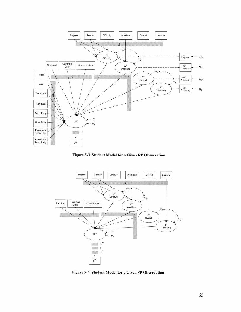
Degree Gender Difficulty Workload Oeal Lcue

D*

Difficulty D/ y D

CommonRequired Core Concentration W* __ )RP wWorkload Workload--- ----

Math

~ Overall - - - - -l )Lab

Teaching TTerm Late

Hewuire

Term Early

Figure 5-3. Student Model for a Given RP Observation

Degree Gedr Difficulty Workload Oeal Lcue

D*Difficulty

00 ------

R Fiuurre 5Cmm .CSetudeint MoeWo * ienS bevto

0*Overall

r

T*

Teaching

IUSP

SP

Figure 5-4. Student Model for a Given SP Observation

65

The behavioral hypothesis is that students rate how recommendable a course is based on

attributes and characteristics relating to their demographics and to the RP and SP

situations.

5.2.1. Latent Attributes

For a given survey respondent, ratings for teaching, overall impression, difficulty and

amount of workload required is obtained from two different sources: (i) average ratings

coming from the evaluation forms of 'The Underground Guide'; (ii) individual ratings

which are collected by the online survey.

Typically, ratings from these two sources differ since the former one represents an

aggregate measure of the impression of an entire class, while the later one is just one

element of this aggregate measure. Moreover, it was found the averages of the personal

ratings for a given class in a given term differed from the averages given by the

evaluation forms for the same class (bias not only exists on an individual level, but is also

found on an aggregate level). This difference in averages can be explained by two

reasons: the survey takers are a subset of the overall students who gave their ratings in the

evaluation forms; the survey takers rated the attributes differently than when they rated

the same ones in the evaluation forms.

The model is ultimately intended to predict the level of recommendation for courses that

have not already been taken. Under this circumstance, individual ratings for course

attributes are unknown for future classes. Only ratings from the evaluation forms can be

explicitly included in making this kind of prediction. On the other hand, individual

ratings for courses already taken are useful for estimating the bias of a given survey taker

with respect to the average ratings coming from the evaluation forms. In terms of

modeling, teaching, overall impression, difficulty and workload were identified as four

different latent variables with average ratings being used as observable variables and

individual ratings being used as indicators of those four latent variables. Note that a given

respondent gives both RP and SP data. Figure 5-3 shows RP observations, and Figure 5-4

shows SP observations (typically a given respondent would have many RP and many SP

observations). Since SP data are not actual courses that have been taken and hence don't

66

have ratings from evaluation forms, there are no indicators for the SP model as shown in

Figure 5-4.

The timing variables are RP specific as shown on Figure 5-3. The two other RP specific

factors are dummy variables indicating whether a course is classified as an EECS math

course (6.041 and 6.042) or an EECS lab (from 6.100 through 6.182). The "Common

Core" included in the RP and SP model is a dummy variable indicating whether a course

belongs to the 4 EECS core courses (6.001, 6.002, 6.003, and 6.004) that all EECS

students have to take independently of the degree they seek.

A different scaling factor is calculated for the RP and SP data (pRP is normalized to 1),

resulting in:

Variance(ERP) = SP Variance(esp

Finally an SP specific constant is estimated resulting in a shifted threshold ?1 with

respect to the RP thresholds ? .

The preliminary studies and analysis of the survey data shows a high correlation between

the teaching and overall rating attributes on one hand and between the difficulty and

workload attributes on the other hand. Based on these findings, the covariances of the

error terms between oh- and af, and between ft and ftw are included in the model

estimation (shown as a two way arrow in Figure 5-3 and Figure 5-4).

5.2.2. Intermediate Models

The joint model presented in both Figure 5-3 and Figure 5-4 was reached after improving

on simpler models that didn't include latent variables. One of those basic models and its

improvement by including the latent variables are presented in Appendix E. The

inclusion of latent variables turned out to significantly improve the goodness of fit of the

model as shown when comparing the rho-bar-squared" in Table E.1 and Table E.2.

Moreover, the final model only incorporated parameters (coefficients or variances) that

p 2 is an index similar to p 2 , but adjusted for number of parameters estimated by the model. In general,

we should prefer models that are parsimonious, i.e., where we do not include variables that contribute very

little to explaining the observed choices. p2 in is an index of incremental explanation provided by the

selected model in comparison to a naive model in which all parameters are set to 0.

67

turned out to be statistically significant. The estimation results for the final model are

presented at the end of this chapter in section 5.4.

5.3. Student Model Estimation

5.3.1. Likelihood Function

The general formulation of the likelihood function given in Equation [5-32], when

applied to the joint model given in Figure 5-3 and Figure 5-4, should incorporate the

following simplifications:

" The model has four latent variables (indexed l=1,..,4) with one indicator for each

one of them. Since we have one indicator for every latent variable, all the a

coefficients were set to 1 for identification purposes. Moreover the indicator index

m is replaced by 1. Indicators are only available in RP situations, hence dropping

the measurement equation for the SP model.

" The coefficients 8 were estimated as being fixed (as opposed to having , and a

distribution of f (6) as in Equation [5-32]).

" VRP and v sp were estimated as having the same distribution v ~ N(O, op).

" The timing variables and the "Math" and "Lab" dummy variables are only present

in the RP setting making them RP only variables. Besides rsp, there are no SP

only variables (no Z to estimate).

Latent Variables

Equation [5-18] defined the structural equation for latent variables as:

X *, =X nA, + F l{

The model shown in Figure 5-3 and Figure 5-4 contains four latent variables with a

covariance matrix Z,, given by:

68

11 12 0 0 Index I Latent Variable

62 -22 0 0 1 Teaching,where 2 Overall

S 0 0 0733 U34 3 Difficulty

L 0 0 0743 r44j 4 Workload

and 72 =721 and 0734 = £743. The restricted form of 1, was explained in section 5.2.1

where it was discussed that the preliminary studies and analysis of the survey data only

shows a high correlation between the teaching and overall rating attributes on one hand

and between the difficulty and workload attributes on the other hand. In this case, the

parameters of the Cholesky decomposition of 1, are:

Fi 0 0 0

]F=21 ]22 ] , where FF'=z0 0 F3 3 0

L0 0 F43 T44_

n, is still defined as an (L xl) vector of standard independent normally distributed

factors:

[1nt2nt

= 2nt where ,Int ~ N(0,1)

L 44nt]j

and F, is the tl row of an (L x L) identity matrix. Taking a concrete example of 1=2

("Overall" latent variable), the structural equation given by X*, =X , + FF{

becomes:

69

0 0 0 ] nt

x X2 ~{±T21 T22 0 0 H2ntX 2nt 2nt Az + F2 (nt X 2 nt2 + [0 1 0 01 ] T3 0 nt

0 0 F43 44 _ 4nt

11 lnt

=X2ntA2 +[0 1 0 0] L I17 3T, t

43;3nt + F4 4 nt

= + 211nt + 7(2nt

Having defined our latent variable structural equations for our model, we can use the

utility of the choice model given by Equation [5-22] for L = 4:

4

U,, = X,,, + (XA+ F1rt )Y,1 , y+o,' + e, ,

When adapted to the model given in Figure 5-3, the RP choice model given in Equation

[5-26] for a given observation r (remember that the subscript t is replaced by r for RP

observations and s for SP observations) becomes:

PRP (YRP | X *,.,W, ; ' ,, yo, r, o-

[5-35] =j=1 (X,,pi+Wnr + (XInrAl + F rnr~ri+ -i.-'ri)

x1+e 'R!P

14

(X n nr S+ (X nrA + F, r4n rri + g,, -ini)

1+e

Introducing indicators and integrating over the latent variables leads to the following RP

likelihood:

pFRP(YRP iRPIX,,,;/,z,6,y,c-,,2L x,)

[5-36] =j j PjRr '(y YT nr| X r ,.,RWn,0;pIr,y , Af Yr=

4 iRP - AX l +FT (RP R

xF r nr jx I nr )dI =1 'T,, U=1

70

Following the same steps and noting that there are no indicators for the SP situations, we

obtain the following SP likelihood equation for the model given in Figure 5-4:

PSP ( SP IX , ; ,-' ,r, rSP , a SP , 2, o)

[5-37] - SJ (yY' x 4 1 9 nsd;fIffffPSP (ns Xn { n ,W ,7n; AT 1r,',y7v ,Ao)X $("dS =1 1=1

The last step is to combine both the RP and SP model and integrate over the panel data so

that the likelihood function for the model can be written as:

p(yRP SP RP I X ,W ;l, ,IsP , esP

[5-38] =j PRP (YRP iRP X W,,~,,~yA,z ,,,

X PnSP (YSPXn I ~7;/,r,, SPIA11,)x )di7

5.3.2. Maximum Simulated Likelihood

Each factor { and i7 introduces a dimension to the integral, making the dimension of

our likelihood function to be 5. We use the Maximum Simulated Likelihood (MSL)

methodology to estimate the unknown parameters of the integrated model. The

simulation procedure will include drawing from the distribution of 4 to simulate the

latent variables, and drawing from the distribution of i7 to simulate the panel data effect.

Latent Variables

Simulation is performed by taking D random draws from the distributions of 4in, 2nt'

3nt and 4 4nt for each observation in the sample (for each RP and each SP observations

hence using the subscript t), denoted ,, , , and ,, d=1,...,D. The structural

equation for latent variable 1 is then written as:

X*d =XtucTua he n

The simulated structural equation is then replaced in the choice and measurement model.

71

Panel Data

Simulation is performed by taking random draws from the distribution F, for each

respondent in the sample denoted i7,d , d=1,...,D. Note that only one draw is taken for all

the observations coming from a given respondent n as opposed to taking one draw for

every observation as was the case for the latent variables. By using this procedure, we

ensure that the panel effect across observations given by a respondent n is taken into

consideration. The utility of the choice model given by Equation [5-22] is rewritten as:

4

Un n= Xj, + X + FF'd )+ond + ent

and the overall likelihood function given in Equation [5-38] for a given draw d is written

as:

Pd (YRP, YSP, RP,| X,W,{ ,Vdj&rZI (5SP SP 9)9 VIPWly-77

Simulated likelihood

The following is then an unbiased simulator for Equation [5-38]:

yRP 1SP RP,(X,W;,,SP 1, jd;SP , r[5-39] D D PS

=- pd( RP P jRP j,,dj~d~f,-II 05P SP A vy,.Y 7D d=v

The parameters are estimated by maximizing the simulated likelihood over the unknown

parameters. There has been a lot of research concerning how to best generate the set of

random points (see [Bhat, 2000] for a summary and references). Numerous procedures

have been proposed in the numerical analysis literature for taking "intelligent" draws

from a distribution rather than random ones. The procedures offer the potential to reduce

the number of draws that are needed for mixed logit estimation, thereby reducing run

times, and/or to reduce the simulation error that is associated with a given number of

draws. Using Halton sequences for mixed logit estimation is one such procedure that we

used to simulate our likelihood function. For more information on Halton draws see

[Bhat, 2000] and [Train, 1999].

72

5.3.3. Estimation with STATA

There are many existing software programs that deal with estimating advanced discrete

choice models. BIOGEME (http://roso.epfl.chlbiogeme) is one software package

designed for the maximum likelihood estimation of Generalized Extreme Value Models.

BIOGEME, however, cannot estimate ordered models. STATA (http://www.stata.com/)

and SAS (http://www.sas.com/) are statistical packages that have routines for estimating

regressions and discrete choice models, but they don't include prepackaged routines to

estimate such a complex model as ours. GLLAMM (http://www.gllamm.org/) is a

program that runs in STATA and estimates "Generalized Linear Latent And Mixed

Models". This program can estimate models with latent variables, random coefficients,

and ordered data. The program, however, uses numerical integration to estimate the

likelihood function. This makes it unusable to estimate models as the one given in

Equation [5-38].

STATA is extensible and can be programmed to compute user-defined maximum

likelihood estimators. We developed a STATA routine to specifically estimate the

likelihood equation given in Equation [5-38]. The routine applies the simulated maximum

likelihood method using Halton sequences as described in the previous section. The code

for the algorithm is included in Appendix F. Details on how the numerical maximization

is performed in STATA can be found in [Gould et al., 2003]. Appendix F contains the

code for the following two core STATA files:

combinedmodel.do

This file loads the data and launches the program by calling other routines. The data is

loaded by first reading the survey database file described in section 4.2.3. It then loads

the Halton sequence that the simulation uses. We wrote a Java program that generates

5000 draws for as many Halton sequences as needed and stores the sequences in a text

file. The STATA program reads this created text file to load the Halton Sequences. Other

routines that are called are:

- datacorrections.do eliminates observations coming from students with no RP

data and corrects the ratings for two courses.

73

- rpjdata.do, sp-data.do, demographics.do setup the variables for the RP, SP and

demographic data respectively.

" interactions.do creates interaction variables such as a match between subject

concentration and student's interest in the concentration.

" combined.do combines the data from the RP and SP experiments

" ologithalton.do is the main routine that simulates the likelihood function

ologit-halton.do

This file implements the core engine of the estimation. The model is specified in the

combinedmodel.do file when calling ologithalton.do. The ologit-halton.do routine uses

the ml command that allows STATA to fit user defined likelihood function. Details on

how to use and program the ml command can be found in [Gould et al., 2003].

5.3.4. Identification

Identification of this complex model is difficult. Applying the sufficient, but not

necessary technique of conditionally identifying each sub-module is not enough to be

certain that the model is fully identified. We used a set of recommended empirical

identification indicators to mitigate this uncertainty (see [Walker, 2001]):

" The parameters converged to the same point and likelihood when given different

starting values.

" STATA automatically verifies that the Hessian of the log-likelihood is non-singular

(a test of local identification). STATA did not issue a "Hessian warning" when it

started crawling toward a solution.

" The parameters were stable as the number of simulation draws increased.

Moreover, STATA's maximum likelihood estimation allows the monitoring of

convergence. The later iterations of maximizing the likelihood of this model followed the

expected pattern of moving smoothly toward a maximum, taking smaller and smaller

steps until the log likelihood function flattened out.

74

5.4. Results

There are a total of 43 parameters to be estimated. That includes: 8 (3 parameters), c (8

parameters), y (4 parameters), r (6 parameters), rsp (1 parameter), yip (1 parameter),

o, (1 parameter), A (9 parameters), 1, (6 parameters including 2 off diagonal

elements), and Z. diagonal (4 parameters). The results are shown in Table 5-2. The

dataset included 1866 RP observations and 1380 SP observations for a total of 3246

observations. Those observations were obtained from 314 respondents. Simulation was

performed using 5000 Halton draws.

This model demonstrates the impact of different course and student characteristics on

students' course ratings. Most of the hypothesis and findings in previous studies were

confirmed. Looking at the choice model (top panel):

- The teaching and overall latent variables both have a significant positive effect on

students' ratings.

- Difficult courses are perceived as being less recommendable.

" Workload, surprisingly, turned out to have a positive coefficient. One would

expect that a higher workload for a given course would lead to a lower rating (and

hence one would expect a negative coefficient), but results showed otherwise.

This can be explained by the fact that course workload is acting as a proxy to the

quantity of information or usefulness of the course, and hence makes the rating

more "recommendable".

m The more the content of a course covers the areas of interests, or

"Concentrations", the more recommendable it is.

m Required courses have a positive effect on rating since required courses are

defined depending on the chosen degree and concentration, and hence are relevant

to a student's interest.

75

- Common core courses, which are requirements for all students, had a positive

effect as well. They are perceived as being essential and useful (and hence should

be recommended to other students).

m Math and Department Lab courses have a significant positive effect on students'

ratings. A note should be made that once these variables, which are RP specific,

were included, the SP constant -rsp became statistically insignificant (as opposed

to be significant with a value of -0.49 in Table E.2). Hence, students particularly

enjoy math and lab courses. Since these factors are not included in SP situations,

student on average rated SP courses 0.49 points lower than RP courses when

those factors were not taken into consideration in RP situation (as was the case in

the model presented in Table E.2).

" As expected, higher ratings of the prerequisites of a given course lead to a higher

rating for that course.

" As far as timing is concerned:

- an elective course that is taken in a later term than its expected average term tends

to have a positive effect on rating, but then this effect decreases proportionally to

how late the course is actually taken. In other words: a given elective course taken

on a later term becomes more enjoyable as students would have the skills and

knowledge maturity to enjoy the course more thoroughly. But taking the course

"too late" is not as recommendable as other courses might depend on it.

- An elective course that is taken earlier than expected tends to get a higher rating.

Those courses can be seen as being particularly relevant to a certain interest area

or concentration, and hence are recommended to be taken as early as possible.

- Finally a required course not taken when it is expected to be has a negative effect

on rating.

Looking at the Latent Variable model (middle panel), the estimated covariance between

teaching and overall rating on one hand, and between workload and difficulty on the

other hand turned to be statistically significant. Results indicate that gender and type of

degree tend to have a significant effect on how workload and difficulty are perceived.

76

Female students tend to rate the workload of a given course higher than male students

would. EE'2 and EECS13 students tend to rate workload and difficulty of a given course

higher than CS1 students would.

The model, shown in Table 5-2, concludes the third step of our recommender system

framework. As was shown in the result discussion, the model is intuitive, behaviorally

realistic and led to insights on which factors are important to students. Attributes that

were included in the choice model are either easy to collect or are readily available online

for upcoming courses making the model particularly suitable to predict courses that

haven't been taken yet. The next chapter uses this model as the backbone of the

recommender engine that the software package uses to predict student ratings.

1 Electrical Engineering13 Electrical Engineering and Computer Science14 Computer Science

77

Table 5-2. Estimation Results (5000 Halton Draws)

Choice ModelCourse Utility Est. , S, y,t t-statT*: Teaching (Latent) 0.39 8.410*: Overall 0.54 9.98W*: Workload 0.37 2.75D*: Difficulty -0.11 -2.33

Concentration 0.20 7.69Required 0.24 7.76Common Core 0.26 -3.94

Term Late 0.94 3.81How Late -0.18 -1.95How Early 0.15 1.98Required x Term Early -0.59 -3.69Required x Term Late -1.06 -4.72Mathematics 0.81 4.49Department Lab 0.79 8.63Prerequisites 0.06 3.13

Tsp (SP constant) -0.11 -0.67ISP (SP constant) 0.60 25.25v, (Variance of Panel Data) 0.11 2.24

Ti 2.28 5.78T2 3.60 9.04T3 4.43 10.97T4 5.34 12.99T5 6.43 15.27T6 7.73 17.82Rho-bar Squared 0.452

Latent Variable ModelStructural Models Est. X, L t-statTeaching Lecturer 0.93 117.48

Variance or 0.31 13.66

Overall Overall 0.95 121.75Variance wo 0.31 10.88

Covariance ooro 0.32 15.28

Workload Workload 0.44 31.84Female 0.15 4.82Degree EE 0.33 5.81Degree EECS 0.46 13.77Variance ow 0.13 27.86

Difficulty Difficulty 0.87 56.93Degree EE 0.13 1.24Degree EECS 0.58 5.50Variance woD 0.35 11.23

Covariance (OWD 0.16 6.96

78

Measurement Model Est. Y, t-stat

ILecturer Variance lIT 1.35 59.69

IOverall Variance Tio 1.28 60.08IWorkload Variance Tjw 0.27 55.31IDifficulty Variance TID 1.08 57.31

79

Chapter 6: Online Academic Advisor

The fourth and final step of the recommender system framework is to implement the

choice model estimated in Chapter 5 as part of the software package that delivers

recommendations. One of the many modules of this software package hosts this initial

model, while other modules are targeted at collecting data, updating the model,

calculating predictions and presenting recommendations. The chapter focuses on

describing this modular architecture by explaining the functionalities and mechanisms of

the different implemented modules in the specific case of our academic advising

application. The chapter also highlights the software package's adaptability and

extensibility to other applications.

6.1. Components of the Online Academic Advisor

Chapter 2 presented the goals and components of a successful recommender system.

A. Choice Set C. Preference Profile for-Books Target User-Products What a system "knows" about- Web Pages a user's preferences- Courses

D.RecommenderEngine that generates

personalizedrecommendations

4Personalized Recommendations

for Targeted User

B. Preference Capture4- How a system learns about

a user's preferences

Figure 6-1. Components of a Recommender System ([ChoiceStream])

80

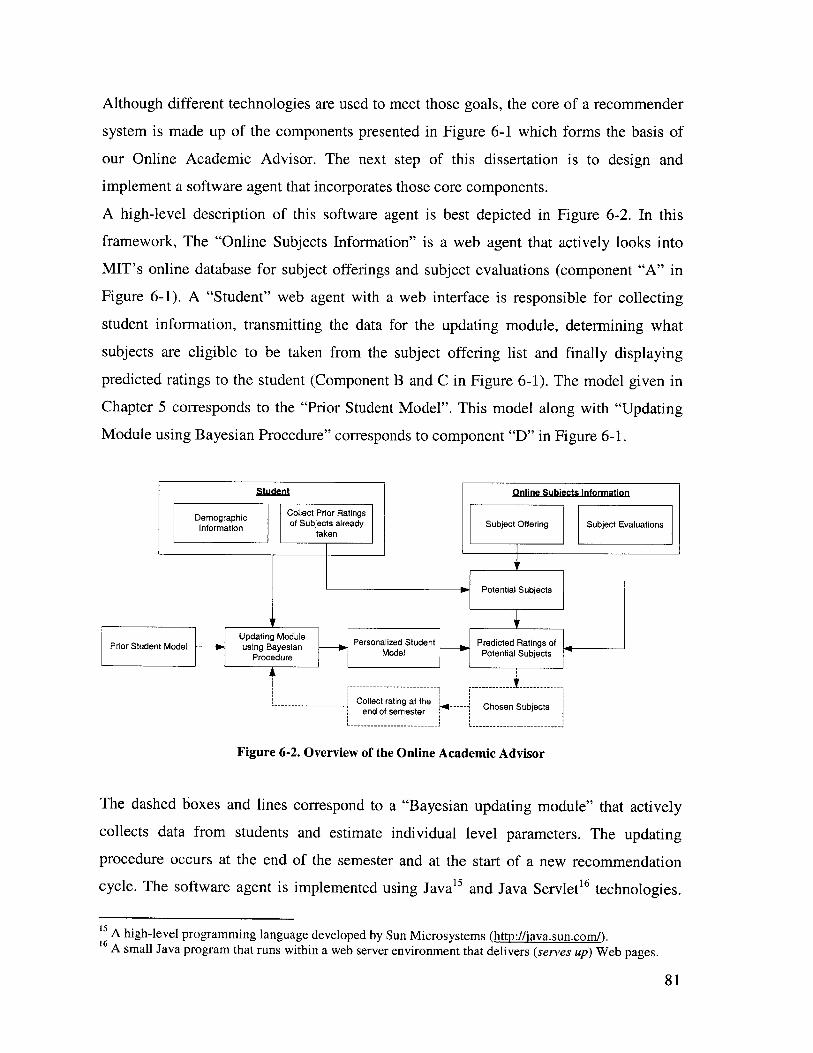
Although different technologies are used to meet those goals, the core of a recommender

system is made up of the components presented in Figure 6-1 which forms the basis of

our Online Academic Advisor. The next step of this dissertation is to design and

implement a software agent that incorporates those core components.

A high-level description of this software agent is best depicted in Figure 6-2. In this

framework, The "Online Subjects Information" is a web agent that actively looks into

MIT's online database for subject offerings and subject evaluations (component "A" in

Figure 6-1). A "Student" web agent with a web interface is responsible for collecting

student information, transmitting the data for the updating module, determining what

subjects are eligible to be taken from the subject offering list and finally displaying

predicted ratings to the student (Component B and C in Figure 6-1). The model given in

Chapter 5 corresponds to the "Prior Student Model". This model along with "Updating

Module using Bayesian Procedure" corresponds to component "D" in Figure 6-1.

Student Online Subiects Information

Collect Prior RatingsDemographic of Subjects already Subject Offering Subject Evaluations

taken

10- Potential Subjects

Updating Module Personalized Student Predicted Ratings ofPrior Student Model using Bayesian Model 10 Potential SubjectsProcedure

Collect rating at the hoseend of semester n Su iet

Figure 6-2. Overview of the Online Academic Advisor

The dashed boxes and lines correspond to a "Bayesian updating module" that actively

collects data from students and estimate individual level parameters. The updating

procedure occurs at the end of the semester and at the start of a new recommendation

cycle. The software agent is implemented using Java5 and Java Servlet16 technologies.

1 A high-level programming language developed by Sun Microsystems (http://java.sun.com/).16 A small Java program that runs within a web server environment that delivers (serves up) Web pages.

81

The rest of this chapter will discuss in detail each of the components of the online

academic advisor.

6.2. Defining the Choice Set

6.2.1. Online Subjects Information

The module acts as a web crawler that collects subject information from MIT's and

Electrical Engineering and Computer Science's websites and constructs a library of

subjects that are either offered in the upcoming academic year or that have already been

given in previous terms. Future subjects are collected from MIT's course catalog for the

current year. Previous subjects along with their evaluation data are collected from the

EECS Underground Guide and are classified by semester. Figure 6-3 shows an overview

of this process.

Subject Manager

Timing Extractor

Collected Data Eubject Semes SubjectConcentration Evaluations

-- l Classifier

Semester Subject

->Guide Extractor

EECS Undegraduate _es Subject

Subject Listingq

MIT Catalog

Figure 6-3. Collecting Data

Guide Extractor is a Java class that systematically go through all the terms of the

'Undergraduate Guide' that are available online. For each semester, a database of the

subjects offered is constructed and is stored in the Subject Manager Java class. The

82

following information is collected for each subject: Lecturers' Ratings, Overall Rating,

Difficulty, Workload, Response Rate and the list of Prerequisites.

Subject Listing is a Java class that goes through the MIT catalog for the subjects that are

offered for the current academic year and extract the list of subjects along with the

term(s) that they are offered.

Concentration Classifier is a Java class that classifies a given subject under at least one

of the seven engineering concentrations that the EECS department offers (see Chapter 1

for a description of those concentrations). To perform its task, this Java class uses the

"Underground Guide" that gives lists of subjects that falls into each of the seven

concentrations.

Timing Extractor is a Java class that uses the survey data (see Chapter 4) to calculate the

average timing of a subject relative to the fall semester of a student's sophomore year

(which is identified as Term 0). A subject taken in the spring of a student's sophomore

year would therefore be identified as Term 1, and so on. The average timing that a given

subject is taken is calculated by averaging the timings from all the students for this given

subject (see "Chapter 4.2.3 Creating the Database" for more details on defining the

timing variable).

The Subject Manager is a key Java class that stores the list of subjects given by the Guide

Extractor and the Subject Listing components, and manages all subject related issues

such as:

" Determining the list of potential subjects that may be taken by a given student

depending whether the prerequisites for the class are satisfied.

" Calculating subjects attributes that aren't constant for all students. More

specifically it determines:

* Timing variables as given in "Chapter 4.2.3" (e.g. student is taking the subject

in a later term than the average term when it's usually taken).

83

" Whether a given subject is a requirement for a given student (this would vary

depending on the degree the student is pursuing17 ).

* The values of the concentration attribute. Students are asked to indicate on a

scale of 1 to 4 the importance, as far as their interests are concerned, of each

of the seven engineering concentrations that the EECS department offers. This

indicator is used to quantify the relevancy of a given subject depending on the

concentration it belongs to. The Subject Manager uses this information to

associate a given subject with the relevancy indicator of the corresponding

concentration for a given student. Take as an example of a student who rated

the "Artificial Intelligence" concentration as 4 ("Essential") and the

"Theoretical Computer Science" concentration as 2 ("Somewhat Important").

A course that falls under both of these concentrations would get a

compounded concentration value of 6 for this student.

6.2.2. Potential Subjects

Defining the set of potential subjects to be taken for a given student is a task that heavily

involves the Subject Manager Java class. Figure 6-4 depicts the process of defining the

choice set (i.e. the list of subjects that a student can take in the upcoming semester) for a

given student.

Given an instance of the Student Java class (i.e. one particular student), the first step in

defining the list of potential subjects that this student can take is to go through all the

subjects that are offered the next semester (Subject Offered in the Subject Manager Java

class) and check whether the student has already taken the prerequisite subjects by

comparing them with the list of subject that the student has already took (Subjects Taken

in the Student Java class).

In case the prerequisites of a potential subject are satisfied, the next step is to describe the

subject using the evaluation forms (setting values for the teaching, overall, difficulty, and

workload ratings). This task is handled by the Evaluation Data for Potential Subjects

method. As a reminder, the potential subject in question, although given in past

17 The degree that a student is pursing is matched with the list of the required classes for that degree. SeeChapter 4.2.3 for more details.

84

semesters, is a future subject that has not been given yet and hence doesn't have

evaluation data from students taking it (e.g. 6.001 in Spring 2004 had an overall rating of

5.5; if the system is trying to recommend this subject for the upcoming Fall 2004, what

would be the overall rating be?). The Subject Manager has a database of the evaluation

data for all EECS subjects that have been given in the last 10 years. These historical data

can be used to estimate the value of the evaluation data for upcoming potential subjects.

There are many ways of using this historical data. One example would be to average the

subject evaluation data for the given course over a certain number of recent semesters.

StudentSubject Manager

Subjects Subjects SubjectTaken Offered Evaluations

Degree PrerequisitesSatisfied

Concentration tRatings V

Evaluation Data for

PPotential Subbjets

Figure 6-4. Potential Subjects

We used a much simpler technique where the evaluation data of the term that the subject

was most recently given is used (in the case of our previous example, 6.001 for the Fall

2004 semester would have an overall rating of 5.5). We chose this technique based on the

assumption that the core material of a subject is usually fairly stable over time; the way

the material is delivered, however, significantly varies. In that case, the most recent

version of the subject would be the most accurate one to describe the same subject that

will be given in the upcoming semester.

85

6.3. Creating a Student Profile

How a system learns about a user's preference and what the system knows about the

user's preferences is a key component to any personalization system (see Figure 6-1

components "B" and "C"). Our online academic advisor tackles this task by explicitly

collecting student's information (demographics such as degree, concentration interest,

etc.), collecting ratings of courses already taken, and using stated preference data to

collect more observations. The task of creating a profile for a given students is divided

into two parts:

m Instantiating a student object from the Student Java class

" Collecting data for that particular student using the Student Controller Java class

that is responsible for displaying and collecting data.

Figure 6-5 shows an overview of the different Java classes involved in creating a student

profile and collecting data.

Figure 6-5. Creating a Student Profile

When a student log-in to the system for the first time, a student object is instantiated. It

will hold the student's profile, information and model. The student model is the discrete

86

Discrete Choice

-- -I ii lM odel

Student

SubjectsTaken

DemographicInformation

StudentControllpr

02

Demographic Subjects Taken Stated PreferenceWebpage Webpage Webpage

Demogiraphic SubjectsSPIfInfo Taken InfoSPnf

_DataCollector

choice model that was constructed and estimated in Chapter 5. A more detailed

description of this model will follow in the next section, but for now it would useful to

mention that the student model is initialized to the average model that was estimated in

Chapter 5. The next step is to collect student information. The Student Controller Java

Servlet class is responsible for collecting data through an abstract Java class called Data

Collector. The Data Collector is either extended as a Demographic info, Subjects Taken

info or SP info Java Servlets depending on the information the Student Controller is

collecting. The Data Collector uses polymorphism1 8 to display different webpages (using

JSP 19 technology) and collect data depending on the class that is extending it. The first

step, as shown in Figure 6-5, is to collect basic demographic information (a snapshot of

the webpage is shown in Figure 6-6). The second step is to collect data on subjects that

have already been taken by the student (as shown in Figure 6-7).

Figure 6-6. Demographic Information

18 In Java, polymorphism refers to the ability to process objects differently depending on their data type orclass (http://www.webopedia.com/TERM/p/polymorphism.html ).19 Short for Java Server Page. A server-side technology, Java Server Pages are an extension to the Javaservlet technology that was developed by Sun.

87

Pg.e f 5

Online Academic Advisor

Section A

Please email bhcmit.edu if you have inquires about any aspects of this survey

1) if you have already chosen an undergraduate degree, which one are you seeking (or have obtained)?

r Course VI- 1/Vi-lA: Bachelor of Science in Electrical Science and EngineeringC Course VI-2/Vi-2A: Bachelor of Science in Electrical Engineering and Computer Science

Course VI-3/Vi-3A: Bachelor of Science in Computer Science and Engineering

2) Please indicate the importance, as far as your interests are concerned, of each cf the engineering concentrations

Not important i Very Important Essential

Communication, Control, and Signal Processing EE) C cArtificial intellgence and Applications (CS) C........... -- . .---- . .-- ----- . . ---. ----Devices, Circuits and Systems (EE)Computer Systems and Architecture Engineerng (GS) i C CElectrodynamics and Energy Systems (EE) C CTheoretical Computer science (CS) C -

Bicelectrical Engneenng (BE) C -

3) What is your current year?

r SophomoreJunior

C SeniorM.Eng, Graduate

4) Were you or are you seeking a double degree?

r Yes; please specify in which department you are seeking your second degreeCNo

Online Academic Advisorsection a

Coaieni Core cathemadsr,

e 00 -fr n prt I ari cAu

6.Nu2 ir-jt W. - -cros~

.......... ~ w , r 0 . .. ..... ......

Camuna n Control, and ranal Devies. a~rut and Siastems

6e3c 7 **""*

6 243yl.1361/16.3371 (il dyn1m 11 VrnnoaY.-ea -i1 dsar.e a t te-nq-e

1 4 5 a 7

rllultf V y xcelentbachbn Poor

Tra oo Too

Overall Ratina xcellent

Average of hoursyou've spent onsubject per week

took tne rse load

to the followiog, you are oskod If YOU Would racomnmend this subject tooa student who resembles you-when you took this class (same background abilities, Interests, and temnperament).

1 2 4 5 h.7Would you Not Highlyrescmmen Recommended Recommended

Figure 6-7. (a) Select Subjects Taken; (b) Rate Selected Subjects

The final step is to complete the data collection by presenting the student with a set of

stated preference questions (see Chapter 4 for more information on how the stated

preference scenarios were designed).

Figure 6-8. Stated Preference Scenario

The more stated preference questions answered, the more data points the system has for

the given student, the better an idea the system will have about the student's preferences.

88

4, Which subject would you prefer if you had to choose between Subject A and Subject B?Click on the attribute to get a detailed explanation In a separate window

scued orblective?Required class has no Required Electivealtemative substitute

Common Core or one of Electrodynamics and Energy Computer Systems and ArchiteclSystems Engineering

Cthe v at

Overtaliiultte f very23 4.5 6.7ve ery1132b3 4 56c cllpoarflmflflfl Excelen

t Ennnr-n-nMo cEll

5v~raliIIt* Tao 123456 7 Too Too 1 2 3 4 5 6 7 ToEas E Difficult Easy Diffic

Overal Ratn very 1 2 3 4 5 6 7 Very 1 2 3 4 5 6 7Poor rnlflflf

t Exclent PoorfE cell

Workload$ypaof hours/weekspent an subject (Bothsubjects are 12 credits)

Overall course toad ofyour semester L o h

Which subject would you prefer? (1- Defnitely A; 4-Na preference 7-Definitely B)

1 2 3 4 5 6 7Definitelyr Dohntoly

A B

There is a balance between asking too many questions to increase the accuracy of

predictions, and too few questions to minimize the time spent answering the

questionnaire. Finding the optimal number of stated preference questions (which will

probably vary depending on the student) is a problem that will not be tackled by this

dissertation. Based on findings in Chapter 4, five stated preference questions are used by

the Online Academic Advisor.

6.4. Recommender Engine

One of the goals of this dissertation is to create a generic framework to use discrete

choice models as the core engine for giving recommendations. In order to achieve that, a

Java package that contains a set of Java classes that defines the behavior of a discrete

choice model was created. The class diagram is shown in Figure 6-9.

DCM-categories : java.util.Vector Parameter

+addParameter(in category_name : String, in parameter: Parameter) -name: String+addCategory(in name : String) -mean: double+getParameter(in Name : String) : Parameter -std deviation : double avautil.Veotor+setParameter(in name: String, in parameter: Parameter) -parameter_counter: static int+getNumPar( : int +setValues(in parameter: Parameter)

StudentModel LatentVariable ParVector-gammas: ParVector -name : String

+calculateUtility(in student : Student, in subject: Subject) : double -indicator sd : Parameter +parameterAt(in index: int) : Parameter+orderedLogit(in student : Student, in subject: Subject) : int +addGamma(in parameter: Parameter) +getNameo : String

Figure 6-9. Class Diagram of Discrete Choice Model

Parameter Java class is the building block of this package. This class defines a random

coefficient parameter by giving it a name and a distribution (mean and standard

deviation). A parameter with a fixed coefficient has its standard deviation set to 0.

ParVector Java class extends the Vector Java class and is used to store a collection of

parameters. This is particularly useful when storing a set of parameters that act

collectively. One such example is the set of explanatory variables for a given latent

variable where these variables are used to give an estimate of the latent variable that will

enter the utility function (see Chapter 5.1.5). A given parameter can actually belong to

several ParVector Objects. Reusing our latent variable example, one explanatory variable

89

can be part of the latent variable model as well as directly contributing to the utility

function and being part of the choice model (See Figure 5.2).

LatentVariable Java class extends the Parameter class. In addition to the distribution of

the latent variable (mean and standard deviation) that are inherited from the Parameter

Java class, this class contains a ParVector (called "gammas") that holds all the

explanatory variables of this latent variable parameter.

DCM Java class defines any generalized discrete choice model as defined in Chapter 5.

The categories is a vector of ParVector. Each ParVector defines the different parameters

categories that might exist in a discrete choice model (e.g. Revealed Preference only

variables, Stated Preference only variables, Combined variables, cutoffs for an ordered

model, etc.). The DCM Java class, given the values of the explanatory variables, can

calculate the overall utility of an alternative. By defining a link function (e.g. logit,

probit, ordered logit, etc.), the DCM calculates the probability that a given alternative is

chosen. The DCM uses an internal simulator to simulate the utility function when random

coefficients are involved. The simulation goes as follow:

1. Take a draw 83 d from each random coefficient in the model using its

corresponding distribution.

2. Using #", calculate the probability i< of choosing alternative i.

3. Repeat step 2 for all alternatives i=J,...,J where J is the total number of

alternatives.

4. Repeat steps 1 to 3 many times, with the number of times labeled D. The resulting

1 Dsimulated probabilities are calculated as follows: P =- I Pd

Student Model Java class extends DCM and is used to make the calculations easier for

our Online Academic Advisor problem. It determines how the utility is calculated given a

student and a subject. It also defines the link function (mixed ordered logit) that was

defined in Chapter 5, and the output of the model. For an ordered logit model, there are

90

several ways we can make a rating prediction. For every cutoff in the ordered model, we

calculate the probability of the rating falling within that cutoff point. We can then either:

" Display the rating corresponding to the cutoff with the highest probability

" Display all cutoffs with their corresponding probabilities

" Calculate an expected rating by using: E = iP , where i denotes a cutoff point.

We decided to use the expected rating to give the rating prediction. The orderedLogit

function in the Student Model Java class hence gives the expected rating for a given

subject given a student profile. In the context of the student model and using the utility

given in section 5.3.2:

nt= Xt, + W.,+ (XA, + FT~n,y, + o-n + ent,

pd is calculated as follows:

P~d d XdW,, ,8,1-.1,, y, A, Yw, av

[6-1]

+e(Xn,6+w.,s+ ( I.,A,+FT( y + av -'ri) l+e (X,+WM5+P X nZ +FT , +afd -ri_- )

This leads to:

SD

[6-2] P =- _ pd (i| X.,,Wd dvJD d= 1 "C V

from which E = iPI can be computed.

6.5. Updating Module: Individual-Level Parameters and BayesianProcedures

The final piece of our recommender system is the updating module shown in Figure 6-2.

To capture the differences in tastes among students, a mixed logit model presented in

Chapter 5 was specified. However in order to give personalized recommendations, we

need to determine where in the distribution of tastes does a particular student lie.

91

If we knew nothing about a student's past ratings, then the best we can do in describing

his/her tastes is to say that his/her coefficients lie somewhere in g( 6l 6) (see Figure 6-10).

However, if we have observed that the student gave a rating y when facing situations

described by X, then we can use h(,8 Iy,X, 0). Since h is tighter than g, we have better

information about the student's tastes by conditioning on his/her past choices.

Figure 6-10. Taste variation [Train, 2003]

6.5.1. Conditional Distribution and Conditional Predictions

A student's choices reveal something about his/her tastes which we can discover. There is

a precise way for performing this type of inference, given by [Revelt and Train, 2000]

and [Train, 2003]. The main concept lies in using Bayesian procedures. Prior to

collecting data from an individual student, the recommender's system estimates are based

on past analyses given by a density of 6, called the prior distribution. The recommender

system collects new data from a student in order to improve its ideas about the values of

6. In its most basic form, the utility that student n obtains in situation t is given by:

[6-3] U , = XJ,# + eo, , where /3n - g(,0 1|6),

and 6 are the parameter of the distribution g. Let y,= <ynJ, ... YnT> denote the student's t

sequence of chosen ratings and Xn the collection of X,, for those observations. Similar

to section 5.1.2, we define the ordinal choice indicator as:

y, = , if i < U, i i=1,...,7.

and

1, if y,=Yit=0, otherwise'

92

If we knew ,, then the probability of the person's sequence of ratings would be:

[6-4] P(y, I X,, )

Since we do not know fin, we need to take the integral over the distribution of 8:

[6-5] P(y, IX,,O)= JP(yn |Xn,)g(fi|6)dfi;

The distribution of coefficient for the student giving a sequence of ratings y, when facing

a rating situation described by Xn is derived from Bayes' rule and is given by [Train,

2003]:

[6-6] h(,81 yX ,0)= " P(Y | X,,3) g(3j1)

P(Y yI Xn ,0)

We know all the quantities on the right hand side and g(,| 16) is given from the full

model (Table 5-2). The mean 8 for the new student model would be:

[6-7] , = Jfi.h(,fly, x,,O)dQ

This mean generally differs from the mean j8 in the entire population. Substituting the

formula for h:

[6-8] A =J/. P(Y" X,3) g(,810)d,8

fP(y| IX,,8) g(fi|0)d,8

The integrals in this equation do not have a closed form; however, they can be readily

simulated. Take draws of fi from the population density g (/8 |0). Calculate the weighted

average of these draws, with the weight for draw fid

P(yn I X,, 9/8) . The simulated subpopulation mean is

[6-9] f, =I wd fd

d

where the weights are:

being proportional to

93

t=1 = +"

[6-10] wd _P(yn | Xn, /d)I P(yn I Xn,id)

d

Suppose now that person n faces a new rating situation described by X,, T+1) If we had

no information on the person's past choices, then we would assign the following

probability to his/her rating i:

P(i I X, (T+1)' 0) = fLn(T+l) Xn (T+1) ,8) g (fi I 8)d8,

where:

L = 1 1nT+1> n +1x1 + e(X,(T+1,r) - e(X _T+1),i1)

If we observe the past ratings T of student n, then the probability can be conditioned on

theses choices. The probability becomes:

P(i I Xn (T+1' 0) = + L>n(T+) (W Xn (T+1) ,8) h(,1 y,, X ,0)d#

So instead of using g(#| 10), we mix over the conditional distribution h( I yn, X,, 1 8).

To calculate this probability, we substitute the formula for h from Equation [6-6] and

simulate by taking draws of 8 from the population distribution g(,3 |0). Calculating the

logit formula for each draw and taking a weighted average of the results we obtain:

[6-11] P(i I X(T+l,,)= 1 wLn(T+)i XnIr+>,d

where the weights w are given by Equation [6-10].

6.5.2. Student Model Application

The framework established in the previous section for calculating predictions for a new

situation (T+1) conditioned on previous T observations can be readily applied to our

student model and can be easily integrated in our Java framework using the simulator that

was describe in the DCM Java class.

94

Using Equation [6-1] to get the likelihood function of a student faced by a new situation

(T+J) for a given draw d, and using Equation [6-11] to calculate the conditional

probability, we obtain:

PG|jX'(r.1),Wn(r+1))

[6-12] dp T 1 T+) +1)i() nne d;f, , , g, ,

d

where

d pd n

d

and

Pd (yn |Xn,Wn ,{d ~d. ''W4V

Yint1 1

1 + (X, , +W.,+ X ,A +F T{ ) + u -uv - 1 ( X,,/+W ,S+ ( X In,A, +F1T4 y, +-,f -r _1)1+ e =11+ e 1=1

Hence by using Equation [6-12], the predictions given by the Online Academic Advisor

become personalized as they take into consideration previous ratings given by students.

6.6. Performance of the Online Academic Agent20

6.6.1. Data and Experimental Technique

In order to measure the performance of our recommender system, we divided the

collected data that was used to estimate the model into two datasets; one was used to

estimate the model and the other one was withheld to measure performance. The data

consisted of 3286 ratings from 314 users having at least 5 ratings. 20% of the users (63

users) were randomly selected to be the test users. From the test sample, ratings for 5

items per user were withheld making up a total of 315 observations withheld from the

data (approximately 10%). The quality of a given prediction can be measured by

comparing the predicted values for the withheld ratings to the actual ratings.

20 The notation in Section 6.6 is independent from the general notation of the thesis listed on page 9.

95

6.6.2. Metrics

The problem of developing good metrics to measure the effectiveness of

recommendations has been extensively addressed in the recommender systems literature.

Some examples of this work include [Mooney 1999], [Herlocker et al., 1999] and [Yand

& Padmanabhan, 2001]. However, in most cases, the evaluation of a particular

recommendation algorithm is usually limited only to testing its performance in terms of

the coverage and accuracy metrics. Coverage is a measure of the percentage of items for

which recommendation system can provide predictions [Herlocker et al., 1999]. This

metric is more of a concern for collaborative filtering algorithms where recommending

items is highly dependent on how often a particular item has been rated, or how well it

can be associated with other items in the database. Coverage is not a concern in our

algorithm as each class can be divided into attributes, and hence all classes can be

potentially recommended regardless of whether they have been rated or not. Many

metrics have been proposed for assessing the accuracy of a collaborative filtering system.

In this research, we will be focus on statistical accuracy metrics that evaluate the

accuracy of a filtering system by comparing the numerical prediction values against

student ratings for the items that have both predictions and ratings [Herlocker et al.,

1999].

Correlation between actual ratings and predictions has been commonly used to measure

prediction engine performance [Hill, et al., 1995], [Kautz, et al., 1997], [Sarwar, et al.,1998]. The most common measure used is the Pearson correlation coefficient, this is the

one reported in this dissertation. Pearson correlation measures the degree to which a

linear relationship exists between two variables (see [Shardanand and Maes, 1995] and

[Sawar et al., 1998] for more details). When computed in a sample, it is designated by the

letter r and is sometimes called "Pearson's r". The value of r can vary from minus one to

plus one. A minus one indicates a perfect negative correlation, while a plus one indicates

a perfect positive correlation. A correlation of zero means there is no relationship

between the two variables.

96

6.6.3. Performance with no Conditioning

In order to calculate the Pearson's correlation for the student model, the expected rating

is computed for all the withheld ratings (5 ratings/user for 63 users). The expected rating

is compared to the true ratings to compute r which is reported in Table 6-1 as "Model 1".

Finally, we provide a naYve model ("Model 0") that assigns a correlation between the

overall rating of a course and the true rating on how recommendable a course is. By

calculating this correlation, the model actually measures how predictable

recommendations are by simply taking into consideration the overall rating attribute. This

naive model allows us to benchmark the significantly more complex student model by

computing the correlation improvement.

Table 6-1. Benchmarking The Student Model's Performance

Model Description # of observations/user used from Pearson t-testwithheld data Correlation r

0 NaYve Model 5 31 6.18(total # of obs = 315)

1 Estimated Student Model 5______ without withheld data (total # of obs = 315) .67 15.54

The t-tests2 indicate that the correlations are significantly different from zero at the 5%

level (t-test > 1.96). The student model's performance shows a considerable improvement

over the naYve model (a 116% increase in correlation). Table 6-2 is based on the

methodology and notations described in Appendix G. A correlation coefficient r can be

transformed into a z-score for purposes of hypothesis testing. This is done by using the

following formula:

1 1+rZ=2 1I- r)

The end result is Fisher's z-score transformation of Pearson's r. Fisher's transformation

reduces skew and makes the sampling distribution more normal as sample size s

increases. Using Fisher's z-score, Table 6-2 shows that the difference in correlation is

significant despite the relatively low number of observations.

21 Refer to Appendix G for a description of statistical tests for Pearson correlations.

97

Table 6-2. Significance of Performance Improvement

Model s r z Standard Error of the difference t-test of the difference0 315 .33 .34 .67 4.241 315 .67 .81

6.6.4. Performance with Conditioning

Recall that five randomly chosen observations were withheld from 63 randomly chosen

users. In order to measure the performance of our updating system, we will divide those

five observations per user into two parts:

" u: number of observations used to update the student model.

" p: number of observations used to measure performance (p = 5 - u).

We are also interested in observing the change in performance as u increases. For a given

u, the procedure is as follows:

1. Randomly select u observations out of the 5 withheld ratings per user.

2. Using those u observations, calculate the expected rating for the p observations

using the methodology describe in section 6.5.2.

3. Compute the Pearson's correlation r by comparing the expected ratings with the

true ratings for those p observations.

4. The process is repeated S times and the average and standard deviation of the S

calculated correlations are reported.

The results for u = 1,2,3 and 4 are presented in Table 6-3. The correlation improvement

over the number of updates u is plotted on the chart in Figure 6-11.

Table 6-3. Comparative Performance using Pearson Correlation

Model u S Pearson Std Paired %Correlation r Deviation t-test Improvement

1 0 0 .6722 1 50 .737 .0131 35.3 9.73 2 50 .754 .0126 6.54 2.34 3 50 .762 .0128 3.15 1.15 4 50 .767 .0114 1.71 .66

98

0

00

0.78

0.76

0.74

0.72

0.7

0.68

0.66

0.64

0.62

0 2

# of updates u

3 4

Figure 6-11. Performance vs. updates

The paired t-test was calculated by using the following equation:

,M - r.12 a2M= '+ "'-1

S, S,,_

where: m is the model index,

Sm is the sample size (number of runs the Pearson Correlation

was computed)

F is the average Pearson Correlation over S,

cm is the standard deviation of model m over S,

6.6.5. Performance Discussion

The average student model significantly showed an improvement over the naive model.

In Table 6-3, we see that conditioning on only one observation significantly improved the

model by 9.7%. However, there are strongly decreasing returns to conditioning on more

observations. Conditioning on two observations only improved the correlation by 2.3%

over the correlation obtained from conditioning on one observation, and a mere 1.1%

improvement for conditioning on 3 observations over 2. Finally conditioning on 4

observations didn't significantly improve performance over conditioning on 3

99

-i ,.. .... ...

1

observations. Figure 6-11 shows how the performance graph flattens out as the number of

updating observations increases. There are two reasons that might explain why the

correlation gain from updating was not drastic and was mostly limited to the first

observation.

First, the initial unconditioned average student model captured most of the variation in

taste within the sampled student population. That leads to a stable model where the

performance due to updating rapidly converges.

Second, we did not include in our average model all the attributes of the alternatives that

were presented to students. In particular, we omitted attributes or variances (in case of

random coefficients) that did not enter significantly in the estimation of the population

parameters. Some students might respond to these omitted attributes and variances, even

though they are insignificant for the population as a whole. Insofar as the updating

observations involves trade-offs, the conditional distributions of tastes would be

misleading, since the relevant tastes are excluded or the relevant tastes have been

estimated as being fixed and hence cannot be updated. This explanation suggests that if a

mixed logit is going to be used for obtaining conditional densities for each student, we

might need to include attributes that could be important for some individuals even though

they are insignificant for the population as a whole.

The updating module that was implemented as part of the Java package that was

described in this chapter demonstrates how the distribution of coefficients for an

individual are obtained from the distribution of coefficients in the population. While

these conditional distributions can be useful in several ways, it is important to recognize

the limitation of the concept as was demonstrated when the performance of the updating

module was measured. While the conditional distribution of each student can be used, we

would ideally relate preferences to observable demographics of the students. Those

observable demographics (such as degree, concentration, requirements, gender, etc.)

could be entered directly into the model itself, like we did in Chapter 5, so that the

population parameters vary with the observed characteristics of the students in the

population. In fact, entering demographics into the model is more direct and more

accessible to hypothesis testing than estimating a model without these characteristics. By

100

entering demographics into our student model however, the variability of the distributions

becomes insignificant or limited to a few parameters. This leads to an initial model whose

performance is high, but with limited room for improvement when it comes to updating

with new observations. Although our specific application where a number of students'

characteristics captured most of the variability in rating, this might not be true in other

applications where there will always be great benefits from calculating user's conditional

distributions even after including demographic data, or in applications where there is not

enough information to identify people on the basis of demographics. The conditional

densities would greatly facilitate analyses that have these characteristics.

101

Chapter 7: Conclusion

7.1. Summary and Contributions

Recommender systems represent user preferences for the purpose of suggesting items to

purchase or examine. They have become fundamental applications in electronic

commerce and information access, providing suggestions that effectively prune large

information spaces so that users are directed toward those items that best meet their needs

and preferences. A variety of techniques have been proposed for performing

recommendation, including content-based, collaborative, knowledge-based and other

techniques. One common thread in recommender systems research is the need to combine

recommendation techniques to achieve peak performance. All of the known

recommendation techniques have strengths and weaknesses, and many researchers have

chosen to combine techniques in different ways.

In this dissertation, we investigated the use of discrete choice modeling as a new

technique to constructing recommender systems. The approach was not specifically

intended to overcome the weaknesses of any of the used techniques in the recommender

systems literature, but was rather aimed at investigating and adapting a radically new

model for giving personalized recommendations.

Discrete choice models had proven successful in many different areas and are still subject

to continuous research to extend and enrich their capabilities. This research made use of

the most advanced techniques in discrete choice modeling to develop statistical models

that are behaviorally realistic. It also used advanced simulation methodologies that are

becoming popular in the discrete choice literature to make the models scalable and

estimable in a realistic timeframe. By using Bayesian updating techniques, this research

102

incorporated a learning and personalization effect to the estimated models. Unlike the

estimation of the initial models which is time consuming and is done offline, the

Bayesian updating is fast and can be done online within a timeframe that online users

would expect.

To test the framework of using discrete choice modeling with recommender systems, we

tackled the problem of designing and developing an online academic advisor that

recommends students academic courses they would enjoy. This application is innovative

as no other system that we know of was developed to tackle this problem. The application

also makes use of valuable course evaluation data that is available online for students, but

is not efficiently used. The problem of advising courses is complex and should include

assisting students in choosing which courses to take together and when to take them,

what electives to choose, how to satisfy department requirements, and designing an

extended list of courses that lead to graduation. The recommender system that this

research developed did not aim at fully automating the problem of advising, but rather

focused on developing an online software agent that assists students in assessing how

recommendable a class would be for them to take and hence help them decide which term

to take a required subject and which elective to take. For a given student, the online

academic advisor produced a predicted likeness score for a list of recommended classes.

The recommender system relied on a "student model" that was constructed and estimated

based on a series of surveys and data collected from students. The model statistically

inferred the importance of factors that influence student's overall impression of a class.

Performance of the model was measured based on comparing withheld rating data with

predicted data. The resulting high correlation between actual and predicted ratings

showed that the recommender system was accurate in its predictions. By using the

Bayesian updating techniques to personalize the student models, the correlation between

actual and predicted ratings increased for the first two updating observations, indicating

an increase in prediction accuracy and overall performance. However, the performance

increase, although statistically significant, was modest. Updating with more than two

observations did not improve the overall performance. Two reasons were identified that

might explain why the correlation gain from updating was modest and was mostly limited

to the first observation. First, the initial unconditioned average student model captured

103

most of the variation in taste within the sampled student population. However capturing

taste variations by including specific attributes might be more problematic in other

applications than our academic advising. There will always be great benefits from

calculating user's conditional distributions in these cases. Second, we omitted attributes

or variances (in case of random coefficients) that did not enter significantly in the

estimation of the population parameters. Some students might respond to these omitted

attributes and variances, even though they are insignificant for the population as a whole.

This explanation suggests that we might need to include attributes that could be important

for some individuals even though they are insignificant for the population as a whole.

7.2. Research Direction

The methodology presented here and the empirical case study of recommending courses

to students have brought to the surface the potential for using discrete choice models with

recommender systems. Modeling individual choice behavior as part of an online system

is a relatively new untested method. The design and implementation of an online

academic advisor is innovative and no comparable application is found in the literature.

Both areas require further investigation into numerous issues.

Bayesian Estimation: In this dissertation, the classical method of using maximum

simulated likelihood has been used to estimate the parameter of the student model. A

powerful set of procedures for estimating discrete choice models has been developed

within the Bayesian tradition (details on Bayesian procedures can be found in [Train,

2001]). These procedures provide an alternative to the classical estimation method. The

procedures can also be used to obtain information on individual-level parameters within a

model with random taste variation. The Bayesian procedures avoid one of the most

prominent difficulties associated with classical procedure. The Bayesian procedures do

no require maximization of any function, avoiding the difficulty of solving simulated

likelihood function that can be numerically difficult. Maximum simulated likelihoods

sometimes fail to converge for various reasons. One reason is that the choice of starting

values is often critical, with the algorithm converging from starting values that are close

to the maximum but not from other starting values. The issue of local versus global

104

maxima complicates the maximization further, since numerical convergence does not

guarantee that the global maximum has been attained. For some behavioral models,

Bayesian procedures are faster and more straightforward from a programming

perspective than classical procedures. Developing a module that uses Bayesian

procedures to estimate models would be an important extension to our current

framework. It would avoid the use of computationally slow software tools, such as

STATA, to maximize the likelihood functions. Having this module would hence

complete our framework as a full Java package solution for constructing recommender

systems.

Scalability: Scalability in recommender systems includes both very large problem sizes

and real-time latency requirements. For instance, our recommender system connected to

MIT's web site will get most of its recommendation requests around the same period of

the academic year, probably peaking before the registration day of a given semester. Each

recommendation must be produced within a few tens of milliseconds while serving

hundreds or thousands of students simultaneously. The key performance measures are the

maximum accepted latency for a recommendation, the number of simultaneous

recommendation requests, the number of users, the number of courses available, and the

number of ratings per student.

Effectiveness of recommendations: The evaluation of our recommender system was based

on testing its performance in terms of accuracy metrics. Accuracy was measured

statistically by comparing estimated ratings against actual ratings. Although crucial for

measuring the correctness of recommendations, this technical measure does not capture

adequately "usefulness" and "quality" of recommendations. For example, in our Online

Academic Advisor application, predicting the rating of obvious courses, such as required

courses, might not be helpful to the student. Therefore it is important to develop a

usefulness measure that captures the "academic value" of the recommendations given by

the system. Developing and studying such measures constitutes an interesting research

topic.

105

User Interface: This research heavily focused on the statistical modeling and software

architectural part of the recommender systems. Although effort has been made to make it

architecturally easy to implement web-interfaces, work needs to be done on how best to

present and collect information from students. Examples of important user interface

extensions include:

" Collecting data by designing intuitive and easy to access webpages to inform the

system about one's preferences and personal information.

" Managing student accounts to give the ability to add ratings of courses taken,

change demographic and login information, change some settings such as the

maximum number of recommended courses to give, etc.

" Integrating a planner that would show the schedule of available courses along

with their ratings on a calendar.

m Providing help and detailed explanations on how recommendation is performed

and evaluated. This transparency would help increase the trustworthiness of the

system.

Student Model: The Online Academic Advisor relied on many simplifying assumption to

model students' ratings of subjects. The main assumption was to exclusively focus on

recommending courses in the upcoming semester, ignoring an academic plan for the rest

of the terms. Moreover, the modeling of the interaction between courses taken together or

in a certain sequence over terms was limited. Finally, recommendations were only limited

to courses given in the EECS department while ignoring humanities requirements and

other potential courses given by the rest of MIT's departments. More research needs to be

done in order to relax these assumptions by assisting students in choosing which courses

to take together, what electives to choose, and designing an extended list of courses over

many terms that lead to graduation.

7.3. Conclusion

All existing recommender systems employ one or more of a handful of basic techniques

that have complementary advantages and disadvantages. Modeling what users might like

106

or dislike is clearly complex, and those methods are a simplistic representation of this

behavior. Advancements in discrete choice models offer the tools to improve the

behavioral representation of users' preferences by integrating methods that exploit the

use of different types of data, capture unobserved heterogeneity for all aspects of the

rating process, and explicitly model behavioral constructs such as attitudes and

perceptions. With increasing computational power and increasingly rich datasets, the

framework described in this dissertation can be practically applied to any application and

improve forecasts and predictions of individual ratings and choices. The online academic

advisor that this research developed served as a proof of the flexibility and practicality of

this approach.

107

Appendix A

For a given class, the names, prerequisites, and hours (class, lab, preparation) given are

not the official ones. Instead, what the students surveyed thought was appropriate is

presented. The lecturer listed is the lecturer for the term the subject was evaluated and is

not necessarily the lecturer in the following term. Response rate is the number of

evaluation forms received, and total enrollment for the class is based on post-add date

statistics. "Difficulty" is valued on a scale of 1 (Trivial) to 7 (Impossible), with 4.0 as the

optimal response. "Subject Overall" and "Lecturer Overall" use the same scale. For these

two quantities, a low number indicates a negative response, while a higher one

demonstrates a favorable one.

108

Appendix BThe conjoint analysis part presented students with 15 hypothetical courses with different

levels of the five considered attributes. The respondents had to rank those 15 courses

according to the course they would most likely select. The five attributes were the

following:

" Teaching Style: The style of delivering the content of the course. In particular I

was interested in three lecture styles:

- Lecture (more than 60% of the class consists of lecture)

- Mix (case studies and team projects 40- 60%, lecture 40-60%)

- Case (more than 60% case studies and team projects)

* Instructor Rating: This is an overall rating of the professor giving the course on a

three level scale. Fair, Good, and Excellent. Examples of factors that influence

this attribute are the instructor's teaching skills and experience in the field.

* Workload: The amount of work a student needs to dedicate for the course and the

difficulty of the material.

- Light (requiring less than 4 hours of study per week)

- Medium (4 to 8 hours)

- Heavy (more than 8 hours)

" Content: the level of relevancy of the course content with the student's interests

on a three level scale; high, medium and low.

" Convenience: The convenience of the course from a time schedule and location

point of view. In this questionnaire, a course is rated as either Convenient or

Inconvenient.

109

Appendix C

-I--s ujctASbjc

Covered TopicsCoverage with respect to yourinterests

InstructorOverall teaching skill

KConvenienceIn terms of class schedule

Subject EvaluationEvaluation can come from MIT'ssubject evaluation forms or/andfrom other students

About 500/o of the Less than 30% ofcovered topics are the covered topics are

related to your related to yourinterests interests

Instructor is average Instructor is poor

Inconvenient class Convenient classschedule schedule

Class got average Class got goodevaluation evaluation

WorkloadAmount of work you need todedicate for the subject (assumesubject is listed as 12 credits)

DifficultyDifficulty in terms of understandinglectures, exams and homework

Expected PerformanceSeif-assesment on how well youthink you will perform in this class

11-x;fityIn terms of choosing future classesafter taking this subject

Workload is Light(<9 hours/week)

Class is verydifficult

You expect yourselfto do ok

Is a prerequisite to alot of subjects (gives

you a highflexibility)

Prerequisites You lackClasses and skills required for this confidence in somesubject prerequisites

Workload is Light (<9hours/week)

Class is easy

You expect yourself todo very well

Is a prerequisite to alimited number ofsubjects (doesn't

improve yourflexibility)

You have a solidbackground in all

prerequisites

* Definitely A * Definitely B* Probably A * Probably B

* No Preference

110

-l"AlLy

Table C-1. Description of the Attributes

Attribute Description

Covered A class usually covers several topics. Assume that:Topics - More than 70% of the covered topics are related to your interests

- About 50% of the covered topics are related to your interests- Less than 30% of the covered topics are related to your interests

Instructor The overall instructor's teaching skill is rated on a three level scale: Excellent,Average and Poor.

Convenience In terms or class schedule; an example of an inconvenient course might be:classes on Friday or meeting at 8:30 am. In this survey, a subject is rated aseither Convenient or Inconvenient.

Subject Is what you heard about the class from your fellow students or from the courseEvaluation evaluation forms; in this survey a course can either have:

- a Good evaluation- an Average evaluation- a Bad evaluation

Workload The amount of work you need to dedicate for the subject (assuming the subjectis listed as 12 credit subject). Three levels are presented:- Light (requiring less than 9 hours of study per week for a 12 unit course)- Medium (9 to 15 hours/week)- Heavy (more than 15 hours/week)

Difficulty Is a measure on how difficult the material is in terms of exams and homework;the exams or homework in a class can either be:- Very Difficult- of Medium Difficulty- Easy

Expected Is a measure on how well you think you will perform in a class before actuallyPerformance taking it; in this survey, you either expect yourself to:

- Do very well- Do ok- Do poorly

Flexibility In terms of future classes you might take. A class can be a prerequisite to:- A lot of subjects giving you a high flexibility in choosing your future subjects- A limited number of classes and hence doesn't improve your flexibility infuture subjects

Prerequisites Given a subject with prerequisites, you can consider yourself as either:- Having a solid background in all the prerequisites- Lacking confidence in some perquisites

111

Appendix D

Table D-1. Description the attributes in the revealed preference section

Overall Quality In rating this attribute, please consider the followings:of Teaching - well prepared lectures

- instructor(s) explained clearly and stimulated interest in the subject- instructor(s) encouraged questions and class participation- help was available outside of class for questionsIf more than one instructor, please use this rating as an average of thequality of teaching of all the instructors

Overall Difficulty This rating should be a conglomeration of the level of difficulty of thetext and readings, exams and problem sets. The amount of time spent onthis subject should not be considered a factor in this rating

Overall Rating This attribute can be seen as a conglomeration of:- the quality of teaching,- the difficulty and usefulness of the text and readings- the difficulty and the quantity of exams and problem sets- the pace, workload and organization of the subject- overall value of what is taught or learned

112

6.001 structure and interpretation of computer programs

I completed the class

I eventually dropped the class but can provide some rating; In this case, please provide a rough

estimate of the week of the term that you effectively droppped the class:

SI dropped the class too early to give any rating

F ------------- --- 1 2 3 4 5 6 7

Overall Quality Very Excellentof Teaching Poor

[e; Too v T TooDifficulty Easy Difficult

Overall Rating Por !Excellent

Average # of hoursyou've spent onsubject per week

Terkyou Course load of this

subject term

Grade

In the following, you are asked if you would recommend this subject to a student who resembles youwhen you took this class (same background, abilities, interests, and temperament).

1 2 3 4 5 6 7'

Would youcommend Not Highly

this class? Recommended Recommended

Figure D-7-1. Sample revealed preference question

113

Table D-2. Description the attributes in the stated preference section

Required or Elective?

A required class is a class with no alternative substitute for it; e.g. if you're a 6.1, then the headers of theEE concentrations are requirements.

Engineering Concentration

[Technical area that the subject covers. This can be either a Common Core subject or one of the 7Engineering Concentrations.

Overall Quality of Teaching

This rating takes into account the followings:- well prepared lectures- instructor(s) explained clearly and stimulated interest in the subject- instructor(s) encouraged questions and class participation- help was available outside of class for questionsIf more than one instructor, please use this rating as an average of the quality of teaching of all theinstructors

Overall Difficulty

This rating is an conglomeration of the level of difficulty of the text and readings, exams and problemsets. The amount of time spent on this subject should not be considered a factor in this rating.

Overa Rating

This attribute can be seen as a conglomeration of:- the quality of teaching,- the difficulty and usefulness of the text and readings- the difficulty and the quantity of exams and problem sets- the pace, workload and organization of the subject- overall value of what is taught or learned

Workload

The amount of work you need to dedicate for the subject (assuming the subject is listed as 12 creditsubject).

Semnester Workload

Overa1-1course o'ad osfthe e mes t er you econsidering taking this subject with th__is"_s'_____j__c___

114

Scenario: You still need to choose one more class for your semester. You've reduced your choice set to twosubjects (subject A and subject B). At the end of the day, you will have to choose one of them. You willalways have the chance of taking any of the two classes in a later semester (whether if it is a required or anelective subject).

For every question you should indicate which of the two presented subjects you would prefer. You shouldtreat every question separately.

1 ) Which subject would you prefer if you had to choose between Subject A and Subject B? Clickon the attribute to get a detailed explanation in a separate window

SUbje cts Subje ct A I

'Course Description ,7

Required or Elective?Required class has no Required Electivealternative substitute

ConcntraionComputer Systems and ArchitectureCommon Core or one of Electrodynamics and Energy Systems Engineringthe 7 Q;

COUrse Ev aluat ion IICverall Quality of Very 1 2 3 4 5 6.7 ery 23 4 6 7Teaching Poor Excellent Poor Excellent

Overall Difficulty Too 1 2 3 4 5 6 7Too Too 1 2 3 4 5 6 7 TooEasy f D D Difficult Easy ZD DE E D! Difficult

Overall Rating Very 1 2 3 4 5 6 7 Very 1 2 3 4 5 6 7Poor Excellent Poor EExcellen t

WorS.a

Workload,y; # of hours/week

spent on subject (Bothsubjects are 12 credits)

Semester Workload - --34- -

Overall course load of Low Load High Loadyour semester

Which subject would you prefer? (1-Definitely A; 4-No preference; 7-Definitely B)

1 2 3 14 5 6 7

Definitel 'DefinitelyA 77~

Figure D-7-2. Sample stated preference question

115

Subje ct BI

Appendix EThe base model presented in Table E.1 was reached after estimating similar models that

combined different parameters and eliminating all insignificant factors. In this model, no

latent variables were incorporated in the model. Instead, the "Teaching", "Overall",

"Workload" and "Difficulty" attributes are the values from the evaluation data.

Table E-1. Base ModelChoice Model

Course Utility Est. , 8, X t-statTeaching 0.19 5.23Overall 0.66 7.76Workload 0.192 2.48Difficulty -0.139 -1.94

Concentration 0.12 7.19Required 0.43 6.36

Term Late 1.01 3.71How Late -0.21 -2.21How Early 0.17 2.02Required x Term Early -0.60 -3.71Required x Term Late -1.06 -4.89

Ts1 (SP constant) -0.42 -3.02

ps (SP constant) 0.51 19.25v, (Panel Data) 0.09 2.75

Ti 1.66 7.94T2 3.00 11.32T3 3.94 16.79T 5.04 18.74T5 6.30 21.12T6 7.64 24.94Rho-bar Squared 0.316

The model presented in Table E.2 incorporates the four latent variables described in

section 5.2.1. The incorporation of those four latent variables in the student model

significantly improved the goodness of fit of the choice model. Note that some of this

improvement in fit would probably be captured in the choice model by including in the

base choice model the additional variables that are included in the latent variable

structural model. The rho-bar-squared for the model with latent variables uses the same

degrees of freedom correction as the base model (the 4 attributes were replaced by the 4

116

latent variables), and thus this degrees of freedom adjustment only accounts for the

estimated parameters of the choice model.

Table E-2. Model with Latent VariablesChoice Model

Course Utility Est. X, , X t-statT*: Teaching (Latent) 0.38 8.370*: Overall 0.54 9.95W*: Workload 0.38 2.74D*: Difficulty -0.11 -2.33

Concentration 0.16 6.90Required 0.34 5.14

Term Late 0.93 3.78How Late -0.19 -1.97How Early 0.15 1.98Required x Term Early -0.57 -3.62Required x Term Late -1.04 -4.74

TSP (SP constant) -0.49 -3.55RpP (SP constant) 0.62 25.31v, (Panel Data) 0.12 2.20

TI 2.19 5.69T2 3.48 9.00T3 4.35 10.93T4 5.22 12.93T5 6.34 15.30Rh-bar6 uad 7.70 18.04Rho-bar Squared 0.42 1

117

Latent Variable Model

Structural Models Est. y, a t-statTeaching

Lecturer 0.94 118.45Variance (x>r 0.31 13.64

OverallOverall 0.95 121.75Variance oo 0.33 10.97

Covariance WOT 0.32 15.27

WorkloadWorkload 0.45 31.87Female 0.17 4.90Degree EE 0.33 5.82Degree EECS 0.45 13.79Variance (ow 0.15 27.80

DifficultyDifficulty 0.86 56.95Degree EE 0.13 1.25Degree EECS 0.59 5.52Variance oD 0.36 11.19

Covariance OOT 0.16 6.96

Measurement Model Est. a t-stat

ILecturer Variance lT 1.37 59.85IOverall Variance Uo 1.29 59.92IWorkload Variance uw 0.26 55.27'Difficulty Variance lD 1.12 56.41

The final model that is presented in Table 5-2 incorporates 4 additional factors to the

model presented in Table 5-2. Adding those 4 variables not only improved on the

goodness of fit, but also helped explaining the reason behind students rating SP questions

about 0.5 points lower than RP questions (TsP = -0.49 in Table E.2). More Results

interpretations are provided in section 5.4.

118

Appendix F

combinedmodel.doquietly{clear

set more offglobal Path "c:\documents and settings\bhc\my documents\research\phd\NewQuestionnaire\AnalysiS\STATA\"

global DDraws = 5000global S-seed = 123456789global N-Var = 6

insheet using "${Path}Data\halton_${DDraws}.txt", tab clearsort idsave halton, replace

insheet using "${Path}Data\combinedData.txt", comma clear//insheet using "${Path}Data\synthetic.txt", tab clear

sort idmerge id using haltondrop if _merge == 2

run "${Path}SML\Do Files\data-corrections.do"run "${Path}SML\Do Files\rp-data.do"run "${Path}SML\Do Files\demographics.do"run "${Path}SML\Do Files\sp-data.do"run "${Path}SML\Do Files\interactions.do"run "${Path}SML\Do Files\combined.do"run "${Path}sML\ologithalton.do"}

global SPDATA sp-dataglobal Panel id

//inverse cumulative normal for all the halton draws and assign them to global variableslocal var = 1while 'var'<=$NVar{

local r=1while 'r'<=$DDraws{

qui replace halton-var'var'_iter'r' = invnorm(halton-var'var'_iter'r')global HALTON-var'var'_iter'r' halton-var'var'_iter'r'ocal r = 'r' + 1

}local var = 'var' + 1

}

replace workload = workload/12replace workload~c = workload~c/12

global Teaching teachingglobal overall overallglobal workload workloadglobal Difficulty difficulty

replace how-late = 0 if how-late =.

global Cholesky-Cconstraint drop _all

#delimit ;ml model dO ologit-halton(combined: rating = concentration-c required-c, nocons)(RPOnly: term-late how-early how-late r-term-early r-term-late, nocons)(SP.Only:)(TGamma: teaching-c, nocons)(T-sigma:)(T-sV:)(TBeta:)(0_Gamma: overall-c, nocons)(0_sigma:)(0_SV:)(0_Beta:)(WGamma: workload-c female deg ree-ee deg ree-eecs, nocons)(w-sigma:)(w-sv:)(wBeta:)(DGamma: difficulty-c female degree-ee degree-eecs, nocons)(DSigma:)(DSV:)(DBeta:)

119

(T_0_Covariance:)(wD-Covariance:)(SP-mu:)(Rho:)(cut_1:)(cut_2:)(cut_3:)(cut_4:)(cut_5:)(cut_6:)

#delimit cr

di c(current-date) ": " c(current-time)di "Number of Halton Draws: " $DDrawsml maxdi c(current-date) ": " c(current-time)

combined.do//Combine datagen rating = spreplace rating = rp if rating ==

gen required-c = requiredreplace required-c = sp-required//replace required-c = 0

gen concentration-c = concentrationreplace concentration-c = sp-concentration//replace concentration-c = 0

gen commoncore-c = commoncorereplace commoncore-c = sp-commoncore

gen teaching-c = lecturerreplace teachinqc = sp-teaching//replace teaching-c = 0

gen overall-c = overallratingreplace overall-c = sp-overall//replace overall-c = 0

gen useful-c = usefulreplace useful-c = sp-useful//replace useful-c = 0

gen difficulty-c = course-evaluation-difficulreplace difficultyc = sp-difficulty//replace difficul ty-c = 0

gen workload-c = workload-evalreplace workload-c = sp-workload//replace workload-c = 0

gen termworkload-c = termworkloadreplace termworkload-c = sp-termworkload//replace termworkload-c = 0

if sp data == 0if sp-data == 1

if requiredc ==

if sp-data == 0if sp-data == 1

if requiredc ==

if sp-data == 0if sp-data == 1

if sp-dataif sp-data

if

ififif

== 0== 1teachingc ==.

if sp-data == 0if sp data == 1if overallc ==

sp-data == 0sp-data == 1usefulc ==

ty if sp-data == 0if sp-data == 1if difficultyc ==

if sp-data == 0if sp-data == 1

if workloadc ==

if sp-data == 0if sp-data == 1if workload-c == .

datacorrections.do//data correctionsreplace lecturer1rating = 5.1 if coursenumber == 6034 & term == "Fall 1998"

lecturer1ratinglecturer2ratinglecturer1ratinglecturer2ratinglecturer1ratinglecturer2rating

5.53.85.33.95.53.8

ifififififif

coursenumbercoursenumbercoursenumbercoursenumbercoursenumbercoursenumber

//Drop students with no rp data

ififififififif

ididididididid

2436597394105117

repl acerepl acerepl acerepl acerepl acerepl ace

603360336033603360336033

&&&&&&

termtermtermtermtermterm

dropdropdropdropdropdropdrop

"Fall"Fall"Fall"Fall"Fall"Fall

2001"2001"2003"2003"2002"2002"

120

drop if id ==drop if id ==drop if id ==

185301313

rpdata.do//Required:replace required = -1 if required =.replace commoncore = 0 if commoncore ==replace mathematics = 0 if mathematics ==

//Difficultygenerate difficulty = rp-courses-difficulty

//workloadgen workload-eval = hoursclass + hourslab + hoursprep

//Evaluation forms lecturergen lecturer = (lecturerirating + lecturer2rating)/2 if lecturer2rating != 0replace lecturer = lecturer1rating if lecturer2rating == 0

run "${Path}SML\Do Files\rp-cleaning.do"

//Concentration: replace concentration by ranking importancereplace eci = 0 if ecl ==replace ec2 = 0 if ec2 ==replace ec3 = 0 if ec3 ==replace ec4 = 0 if ec4 ==replace ec5 = 0 if ec5 ==replace ec6 = 0 if ec6 ==replace ec7 = 0 if ec7 ==replace ccsp = 0 if ccsp ==replace aia = 0 if aia ==replace dcs = 0 if dcs ==replace csae = 0 if csae ==replace ees = 0 if ees ==replace tcs = 0 if tcs ==replace be = 0 if be ==

//Department labgen departmentLab = 0replace departmentLab

//Gradesgen grade-scale = 8rep ace grade-scalerep ace grade-scalerep ace grade-scalereplace grade.scalereplace grade-scalereplace grade-scalereplace grade-scalereplace grade-scale

= 1 if coursenumber<=6182 & coursenumber>=6100

=7=6=5=4=3=2=1= 0

ififififififififif

grade =="A+"grade == "A"grade == "A-"grade == "B+"grade == "B"grade == "B-"grade =="C+"grade == "C or below"grade-scale == .

gen grade-given = 1 if grade-scale != 0replace grade-given = 0 if grade-scale == 0

//Termsgen termnum = -10replace term-num =replace term-num =replace term-num =replace term-num =replace termnum =replace termnum =replace term-num =replace term-num =replace term-num =replace term-num =

-8-6-4-20-9-7-5-3-1

gen term-start = 0replace term-start = -2replace term-start = -4replace term-start = -6

ififififififififififif

term==term==term==term==term==term==term==term==term==term==term==

"Fall 1998""Fall 1999""Fall 2000""Fall 2001""Fall 2002""Fall 2003""Spring 1999""Spring 2000""Spring 2001""Spring 2002""Spring 2003"

if year == 1if year ==if year ==if year ==

234

gen term-taken = term-num - term_start

//Concentrationgen concentration = 0

121

repl acerepl acerepl acerepl acerepl acerepl acerepl ace

concentrationconcentrationconcentrationconcentrationconcentrationconcentrationconcentration

//Concentrationgen ccsp-conc = 0replace ccsp-concgen aia-conc = 0replace aia-concgen dcsconc = 0replace dcs-concgen csae-conc = 0replace csae-concgen ees-conc = 0replace ees-concgen tcs-conc = 0replace tcs-concgen be-conc = 0replace be-conc

eci if ccsp ==concentrationconcentrationconcentrationconcentrationconcentrationconcentration

= 1 if ecl >= 3

= 1 if ec2 >= 3

= 1 if ec3 >= 3

= 1 if ec4 >= 3

= 1 if ec5 >= 3

= 1 if ec6 >= 3

= 1 if ec7 >= 3

//Timingsort coursenumberby coursenumber: egen term-avg = mean(term-taken)gen term-timing = term-taken - term-avggen term-timing-int = round(term-timing)

gen term-abs = abs(term-timing-int)

gen

gen

term-early = 0replace term-early = 1 if term-timing-int < 0

term-late = 0replace term-late = 1 if term-timing-int > 0

gen how-early = termabs * term-earlygen how-late = term-abs * term-late

replace how-early = 0 if how-early ==replace how-late = 0 if how-late ==

gen required-temp = 0replace required-temp = 1 if required == 1

gen rtermnearly = term-early * required-tempgen r-term-late = term-late * required-tempgen r-how-early = how-early * required-tempgen r-how-late = how-late * required-temp

drop required-temp

//Prerequisitessort idgen temp =gen avgxen quantity = 0ocal num = 1

while 'num'<=3{qui gen preu_'num' =

local pre.num = 6001qui replace prerequisite_'num' =

prerequisite_ num'>7000

while 'pre-num'<=6400{quietly{

}

replace temp =.replace avgx=.by id: replaceby id: replaceby id: replaceby id: replace Ilocal pre-num =

if prerequisite_'num'<6000 I

= rp if coursenumber == 'pre-num'= sum(temp)/sum(temp !=.)= avx[_NJ_'num = temp if prerequisite_'num' == 'pre-num'e-num' +1

}quietly{

replace preu_'num' = 0 if preu_'num' ==

122

1++++++

ec2ec3ec4ec5ec6ec7

ifififififif

aia == 1dcs == 1csae == 1ees == 1tcs == 1be 1

by id: replace quantity = quantity + 1 if preu_'num' !=0}local num = 'num' + 1

}

gen pre-avg = (preU-1 + preu_2 + preu_3)/quantityreplace pre-avg = 0 if pre-avg == .drop temp preu_1 preu_2 preu_3 avgx quantity

sp-data.do//SP datagen con_1 = 0replace con_1 = eci if concentration1 == 1replace con_1 = ec2 if concentration1 == 2replace con_1 = ec3 if concentration_ == 3replace con_1 = ec4 if concentration_1 4replace con_1 = ec5 if concentration_1 5replace con_1 = ec6 if concentration_1 6replace con_1 = ec7 if concentration_1 7

gen con_2 = 0replace con_2 = ecl if concentration_2 1replace con_2 = ec2 if concentration_2 2replace con_2 = ec3 if concentration_2 3replace con_2 = ec4 if concentration_2 4replace con_2 = ec5 if concentration2 == 5replace con_2 = ec6 if concentration2 == 6replace con_2 = ec7 if concentration2 == 7

gen sp-required = (required_1 - required_2)/2 // Reverse scale to have 1 is required and-1 is electivegen sp.concentration = (con_2 - con_1) +4gen sp-teaching = (teaching_2 - teachingj1 + 6)/2+1gen sp-difficulty = (difficulty_1 - difficulty_2 + 6)/2+1 //Reversed scalegen sp-overall = (overall_2 - overall_1 + 6)/2+1gen sp-workload = ((workload_2 - workload_1 +6)/2+1)*2+6gen sp-termworkload = termworkload_1+1 // Only one termworkload presentedgen sp-heavycourse = (heavycourse_1 - heavycourse_2+6)/2 + 1 // Reverse the scale:consistent with workloadgen sp-useful = (useful_2 - useful_1+6)/2+1

gen sp-commoncore = 0replace sp-commoncore = 1 if concentration1 == 0 & sp<4replace sp-commoncore = 1 if concentration_2 == 0 & sp>4

interactions.dogen workload-term = termworkload * workload // workload nomramlized by load of currentterm

gen sp-workload-term = sp-termworkload * sp-workload // workload nomramlized by load ofcurrent termgen sp-heavycourse-term = sptermworkload * sp-heavycoursegen sp-work-inter = sp-workl oad-term * sp-heavycourse-termgen sp-workload-avg = sp-workload*avg-units/12 //workload normalized by average units persemester

gen overall-teaching = overall * teachinggen overall-useful = overall * usefulgen teachinguseful = teaching * usefulgen difficul1ty-workload = difficulty * workload

gen ccsp-match = 0replace ccsp-match = 1 if ccsp== 1 & ccsp-conc == 1

gen aia-match = 0replace aia-match = 1 if aia == 1 & aia-conc == 1

gen dcs-match = 0replace dcs-match = 1 if dcs == 1 & dcs-conc == 1

gen csae-match = 0

123

replace csae-match = 1 if csae == 1 & csae-conc == 1

gen ees-match = 0replace ees-match = 1 if ees == 1 & ees-conc == 1

gen tcs-match = 0replace tcs-match 1 if tcs == 1 & tcs-conc == 1

gen be-match = 0replace be-match = 1 if be == 1 & be-conc == 1

demographics.doreplace doublemajor = 1 if doublemajor == .replace doublemajor = doublemajor -1 //make

//UROPreplace urop = 2 if urop ==replace urop = 0 if urop == 2 //make it a "0"gen uropreason = 0 if match(urop-reason, "forreplace uropreason = 1 if match(urop-reason,replace uropreason = 2 if match(urop-reason,replace uropreason = 3 if match(urop-reason,gen urop-credit = 0replace urop-credit = 1 if uropreason == 0

it a "0" or "1" variable

or "1" variablecredit")

"for credit and"for pay")""l)

//Employedreplace employed = 1 if employed ==replace employed = employed-1gen employed-offcampus = 0replace employed-offcampus = 1 if employed == 2gen employed-fulltime = 0replace employed.fulltime = 1 if employed == 3

//sleepreplace hourssleep = 6 if hourssleep ==

//Aerepyacereplace

age = 0 if age == .age = age + 14 if age !=0

//Femal egen female = sex-1replace female = 0 ifdrop sex

//internationalgen international= 0replace international

female == .

= 1 if citizenship == 3

//futureplangen future= shorttermplanreplace future = 8 if future ==

gen sophomore = 0 if year != 1replace sophomore = 1 if year == 1gen junior = 0 if year != 2replace junior = 1 if year == 2gen senior = 0 if year != 3replace senior = 1 if year == 3gen meng = 0 if year != 4replace meng = 1 if year == 4

gen degree-ee = 0 if degree != 1replace degree-ee = 1 i degree == 1

gen degree-eecs = 0 if degree != 2replace degree-eecs = 1 if degree == 2

gen work = 0replace work = 1 if future == 6 1 future == 2 1 future == 3

rp-cleaning.do//Drop incomplete observations or term is stated as otherdrop if difficulty == . & sp-data == 0

124

pay")

dropdropdropdropdrop

ififififif

teaching == . & sp-data == 0overall == . & sp-data == 0workload == . & sp-data == 0term == "other" & sp-data == 0term == "" & sp-data == 0

//Drop observations that have a wrong term assigned to themdrop if lecturer == . & sp-data == 0drop if overallrating == . & sp-data == 0

//Drop observations that have lecturer == 0drop if lecturer == 0 & sp-data == 0

drop if rp == . & sp-data == 0drop if sp == . & sp-data == 1

ologit-halton.docapture program drop ologit-haltonprogram ologit-haltonversion 8.1args todo b lnftempvar xb-c xbrp xb-sp lnfjtempname cuti cut2 cut3 cut4 cut5 cut6 rho rho2tempname cov_1_2 cov_3_4 cov2_1_2 cov2_3_4//Latent_1: Teaching Latent_2: Overall Latent_3:Timing

ml evalml evalml eval

mu-sp cons-sp

Workload Latent_4: Difficulty Latent_5:

xb-c'= 'b', eq(1)'xb-rp' = b', eq(2)'xb-sp' = b', eq(3) scalar

local counter 4

local i 1while 'i'<= 4{

tempvar xgi'tempname xb'i' xs2_'i'mleval xgi'' = b,

local counter =mleval 'xs2_'i'' = 'b',

local counter =mleval 'sv2_'i'' = 'b',

local counter =mleval 'xb'i'' = 'b',

local counter =

local i = 'i'+ 1}

sv2_'i' xs'i' sv'i'eq('counter')counter' + 1eq('counter') scalar

counter' + 1eq('counter') scalar

counter' + 1eq('counter') scalarcounter' + 1

local cut-index 'counter'

mleval 'cov2_1_2' = b', eq('cut-index') scalarlocal cut-index = 'cut-index' + 1

mleval 'cov2_3_4' = Ib', eq('cut-index') scalarlocal cut-index = cut-index' + 1

ml eval

ml eval

'mu-sp' = b', eq('cut-index') scalarlocal cut-index = cut-index' + 1'rho2' = 'b', eq('cut-index') scalarlocal cut-index = 'cut-index' + 1

local j 1while j' <= 6{

mleval 'cut'4'' = b', eq(cut-index') scalarlocal j = j + 1local cut-index = 'cut-index' + 1

}

tempname Amat 'A' = 1(9)mat 'A'[1,1] =mat A'[2,2] =mat 'A'[3,3] =mat 'A'[4,4] =mat 'A'[5,5] =mat 'A'[6,6] =

xs2_'xs2_2'xs2_3'xs2_4'sv2_1'sv2-2'

125

mat 'A'[7,7] = 'sv2_3'mat 'A'[8,8] = 'sv2_4'mat A'[9,9] = 'rho2'

mat 'A'[1,2] =mat A'[2,1] =mat A'[3,4] =mat A'[4,3] =

cov2_1_2'cov2_1_2'

'cov2_3_4'cov2_3_4'

capture mat 'cholesky-C' = cholesky('A')

if _rc != 0 {//di "warning: cannot do Cholesky factorization"

scalar 'xs1' = $Cholesky-C[1,1]scalar 'xs2' = $Cholesky-C[2,2]scalar 'xs3' = $choleskyc[3,3]scalar 'xs4' = $cholesky-C[4,4]scalar 'sv1' = $cholesky-C[5,5]scalar 'sv2' = $Cholesky-C[6,6]scalar 'sv3' = $Cholesky-C[7,7]scalar 'sv4' = $Cholesky-C[8,8]scalar 'rho' = $Cholesky-c[9,9]//scalar 'xs-rp' = $Cholesky C[10,10]

scalar 'cov_1_2' = $cholesky-c[2,1]scalar 'cov_3_4' = $Cholesky-C[4,3]

tempvar lasttempvar levell level2 level3 level4 level5 level6 level7 v-rp v-sp v-common lnfjSlnfjAvg

qui{

gengengengengen

gengengengengengengen

doubledoubledoubledoubledouble

doubledoubledoubledoubledoubledoubledouble

'lnfjS' = 0'lnfj' = 0

= 0= 0

v-common' = 0

'levell'=0'level2'=0'level3'=0level4'=0

'level 5'=0'Ievel6'=0Ilevel7'=0

set seed $S-seedlocal repl=$DDraws

local id $Panellocal sp-data $SPDATAsort id'by 'id': gen 'last' = _n == _N

local r=1while 'r'<='repl'{

"ologit-halton"//Hl ton sequence are already normally inversed before calling

id for a given

//Halton sequence are generated by observation for stdN_1 to stdN_4//Halton sequence are generated by id for stdN_5 (one random variable byiteration)tempvar latent_1 latent_1_dist stdN_1tempvar latent_2 latent_2_dist stdN_2tempvar latent_3 latent_3_dist stdN_3tempvar latent_4 latent_4_dist stdN_4tempvar stdN_5

gen double 'stdN_1' = ${HALTON_var1_iter'r'}gen double 'stdN_2' = ${HALTONvar2_iter'r'}gen double 'stdN_3' = ${HALTONvar3_iter'r'}gen double 'stdN_4' = ${HALTON_var4_iter'r'}gen double 'stdN_5' = ${HALTONvar5_iter'r'}

126

//Calculate latent variablesgen double 'latent-l' = 'xgl' + 'xs1' * 'stdN_1'gen double 'latentldist' = normden($Teaching,'latent_1','svl')

gen double 'latent_2' = 'xg2' + 'cov_1_2' * 'stdN_1' + 'xs2' * 'stdN_2'gen double 'latent_2_dist' = normden($Overall,'latent_2','sv2')

gen double 'latent_3' = 'xg3' + 'xs3' * 'stdN_3'gen double 'latent_3_dist' = normden($workload,'latent_3','sv3')

gen double 'latent_4' = 'xg4' + 'cov_3_4' * 'stdN_3' + 'xs4' * 'stdN_4'gen double 'latent_4_dist' = normden($Difficulty,'latent_4','sv4')

replace 'v-common' = 'xb-c' + 'xbl' * 'latent_1' + 'xb2' * 'latent_2' +xb3' * 'latent_3' + 'xb4' * 'latent_4'+ 'rho' * 'stdN_5'

replace 'v-rp' = 'v-common' + 'xb-rp'replace 'v-sp' = 'v-common' + 'xb-sp'

local 1 = 1while 'l'<=6{

replace 'level'l'' = 1 / (1+exp(-('cut'l'' - 'v-rp')))if -sp-data' == 0

replace 'level'l'' = 1 / (1+exp(-'mu-sp'*('cut'l'' - 'v-sp')))if -sp-data' == 1

local 1 = '1' + 1}replace 'level7 = 1 / (1+exp(-('vurp'-'cut6'))) if 'sp.data' == 0replace level7' 1 / (1+exp(-'musp'*(vsp'-cut6))) if spdata' == 1

replace 'lnf' = 'levell' if $MLy1 == 1replace 'lnf = 'level2'-'levell' if $MLy1 == 2replace 'lnfj ' level3'-'level2' if $MLy1 == 3replace 'lnf = 'level4'-'level3' if $MLy1 == 4replace 'lnfi' = 'level5'-'Ievel4' if $ML-y1 == 5replace 'lnfl' = 'level6'-'level5' if $MLy1 == 6replace 'lnfj' = 'level7' if $ML-y1 == 7

tempvar 11.prod temp-prod measurement_1_prod measurement_2_prodmeasurement_3_prod measurement_4_prod

egen double -llprod' = prod('lnfj'), by('id')egen double 'measurement_1_prod' = prod('latent_1_dist'), by('id')egen double 'measurement_2_prod' = prod('latent_2_dist'), by('id')egen double 'measurement_3_prod' = prod('latent_3_dist'), by('id')egen double -measurement_4_prod' = prod('atent_4_dist'), by('id')

gen double 'temp-prod' ='ll -prod'*'measurement_1_prod'* measurement_2-prod'*'measurement_3_prod'*'measurement_4_prod'

replace 'lnf4-s' = 'lnfj-s' + 'temp-prod'local r = r +1

}

gen double 'lnfjAvg' = 'lnfj-s'/'repl'

}mlsum 'lnf' = ln('lnfj-Avg') if 'last' == 1end

127

Appendix G

22This appendix is based on [Chen and Popovich, (2002)] and is dedicated for describing

statistical tests performed on Pearson correlation r.

Si gnificance of r

One tests the hypothesis that the correlation is zero (r = 0) using this formula:

r

t = 1-

s -2

where s is sample size. The computed t value is compared to the critical t value that can

be found in a table of the distribution of t, for (s - 2) degrees of freedom. For large values

of s (> 100), if the computed t value is 1.96 or higher, the difference in the correlations is

significant at the .05 level.

Z-Score Conversions of Pearson's r

A correlation coefficient r can be transformed into a z-score for purposes of hypothesis

testing. This is done by using the following formula:

1 1 + rZ=2 1l.- r)

The end result is Fisher's z-score transformation of Pearson's r. Fisher's transformation

reduces skew and makes the sampling distribution more normal as sample size increases.

z's standard error is given by:

1z =s-

Significance of the difference between two correlations from two independent samples

2 The notation in this appendix is independent from the general notation listed on page 9.

128

To compute the significance of the difference between two correlations from independent

samples, follow these steps:

1. Convert the two correlations to z-scores as outlined above.

2. Estimate the standard error of difference between the two correlations as:

1 1SE= + ,

sI-3 s2 -3

where nj and n2 are the sample sizes of the two independent samples

3. Divide the difference between the two z-scores by the standard error.

t = zi - Z2

SE

If the t value computed in step 3 is 1.96 or higher (if s1>100 and S2 >100), the difference

in the correlations is significant at the .05 level.

129

Bibliography

Adomavicius, G., R. Sankaranarayanan, S. Sen, and A. Tuzhilin. IncorporatingContextual Information in Recommender Systems Using a MultidimensionalApproach, submitted for publication, 2003.

Alspector, J., Kolcz, A., and Karunanithi,N. Comparing Feature-Based and Clique-BasedUser Models for Movie Selection. In Proceedings for the Third ACM Conference onDigital Libraries, pages 11 -18, 1998

Balabanovic, M. and Shoham, Y. FAB: Content-based collaborative recommendation.Communications of the ACM, 40(3), March 1997.

Basu, C., Hirsh, H., and Cohen, W. (1998). Recommendation as Classification: UsingSocial and Content-based Information in Recommendation. In Recommender SystemWorkshop '98. pp. 11-15.

Ben-Akiva, M. and S. Lerman (1985) "Discrete Choice Analysis: Theory and Applicationto Travel Demand", The MIT Press, Cambridge, MA.

Ben-Akiva, M. and T. Morikawa (1990) "Estimation of switching models from revealedmodels with randomly distributed values of time", Transportation Research Record1413, 88-97.

Ben-Akiva, M., J. Walker, A.T. Bernardino, D.A. Gopinath, T. Morikawa, and A.Polydoropoulou (2002) "Integration of Choice and Latent Variables Models", InPerpetual Motion: Travel Behaviour Research Opportunities and ApplicationChallenges (Elsevier Science, Mahmassani, Ed.), Chapter 21, 431 - 470.

Bentler, P.M. (1980) "Multivariate Analysis with Latent Variables", Annual Review ofPsychology 31, 419-456.

Bhat, C. (1999) "An analysis of evening commute stop-making behavior using repeatedchoice observation from a multi-day survey", Transportation Research B33, 495 -510.

130

Bhat, C.R. (2000) "Quasi-Random Maximum Simulated Likelihood Estimation of theMixed Multinomial Logit Model", forthcoming, Transportation Research.

Bhat, C.R. "Quasi-Random Maximum Simulated Likelihood Estimation of the MixedMultinomial Logit Model", forthcoming, Transportation Research.

Billsus, D. and M. Pazzani. User modeling for adaptive news access. User Modeling andUser-Adapted Interaction, 10(2-3):147-180, 2000.

Bolduc, D. (2003) "Simulation-Based Econometric Estimation of Discrete ChoiceModels", University Laval.

Breese, J. S., Heckerman, D., and Kadie, C. Empirical Analysis of Predictive Algorithmsfor Collaborative Filtering. In Proceedings of the 14th Conference on Uncertainty inArtificial Intelligence, pp. 43-52, 1998.

Burke, R. Knowledge-based recommender systems. In A. Kent (ed.), Encyclopedia ofLibrary and Information Systems. Volume 69, Supplement 32. Marcel Dekker, 2000.

Chen, P. Y. and P. M. Popovich (2002). Correlation: Parametric and nnparametricmeasures. Thousand Oaks, CA: Sage Publications.

Claypool, M., A. Gokhale, T. Miranda, P. Murnikov, D. Netes, and M. Sartin. Combiningcontent-based and collaborative filters in an online newspaper. In ACM SIGIR'99.Workshopon Recommender Systems: Algorithms and Evaluation, August 1999.

Claypool, M., Gokhale, A., Miranda, T. Murnikov, P., Netes, D. and Sartin, M.Combining content-based and collaborative filters in an online newspaper. ACMSIGIR Workshop on Recommender Systems - Implementation and Evaluation, August19, 1999.

ChoiceStream. Comparing Collaborative Filtering and Attributized Bayesian ChoiceModeling. Technology Brief.http://www.choicestream.com/pdf/ChoiceStream TechBrie f pdf

Dahan E., John R. Hauser, Duncan Simester, and Olivier Toubia, Application and Test ofWeb-based Adaptive Polyhedral Conjoint Analysis, Unpublished, May 28 2002.

Dahan E. and John R. Hauser, The Virtual Customer, Journal of Product InnovationManagement, 2001.

Dekhytar, A. and Goldsmith, J. The Bayesian Advisor Project. Unpublished, March 152002.

131

Gould, W., J. Pitblado, and W. Sribney (2003). Maximum Likelihood Estimation withStata, Second edition, Stata Press Publication.

Gourieroux, C. and A. Monfort (1996) Simulation-Based Econometric Methods, OxfordUniversity Press.

Hensher, D. and M. Bradley (1993), "Using stated response data to enrich revealedpreference discrete choice models", Marketing Letters 4, 39 - 152.

Hensher, D., J. Louviere, and J. Swait (1999), "Combining sources of preference data",Journal of Econometrics 89, 197 - 221.

Herlocker, J., Konstan, J., Borchers, A., and Riedl, J. (1999). An Algorithmic Frameworkfor Performing Collaborative Filtering. In Proceedings of ACM SIGIR'99. ACMpress.

Huber, J. Train, K. On the Similarity of Classical and Bayesian Estimates of IndividualMean Partworths. Marketing Letters 12:3, 259-269, 2001.

Keesling, J.W. (1972) Maximum Likelihood Approaches to Causal Analysis, Ph.D.Dissertation, University of Chicago.

Louviere, J.J., D.A. Hensher and J.D. Swait (2000) Stated Choice Methods: Analysis andApplication, Cambridge University Press.

McFadden, D. (1974) "Conditional Logit Analysis of Qualitative Choice Behavior",Frontiers of Econometrics, P. Zarembka, Ed., Academic Press.

McFadden, D. (1989) "A Method of Simulated Moments for Estimation of DiscreteResponse Models without Numerical Integration", Econometrica 57(5), 995 - 1026.

McFadden, D. and K. Train (2000) "Mixed MNL models of discrete response", Journalof Applied Econometrics 15, 447 - 470

Miller, B. N., J. A. Konstan and J. Riedel (2004) "PocketLens: Toward a PersonalRecommender System", ACM Transactions on Information Systems, Vol. 22, No. 3,July 2004, 437 - 476.

Mooney, R. J. Content-based book recommending using learning for text categorization.In ACM SIGIR'99. Workshop on Recommender Systems: Algorithms and Evaluation,1999.

Olivier Toubia, Duncan I. Simester and John R. Hauser "Fast Polyhedral AdaptiveConjoint Estimation". Unpublished, February 2002.

Personalization Consortium. http://www.personalization.org/personalization.html

132

Pazzani, M. A framework for collaborative, content-based and demographic filtering.Artificial Intelligence Review, pages 393-408, December 1999.

Resnick, P. and Varian, H. Recommender systems. Communications of the ACM,40(3):56-58, 1997.

Resnick, P., Iacovou, N., Suchak, M., Bergstrom, P., and Riedl, J. (1994). GroupLens: AnOpen Architecture for Collaborative Filtering of Netnews. In Proceedings of CSCW'94, Chapel Hill, NC.

Revelt, D. and K. Train (2000), 'Specific taste parameters and mixed logit', WorkingPaper No. EOO-2 74, Department of Economics, University of California, Berkeley.

Russel, S. Norvig, P. Artificial Intelligence: A Modern Approach. Prentice Hall series inArtificial Intelligence, 1995.

Sarwar, B. M., Karypis, G., Konstan, J. A., and Riedl, J. (2000). Analysis ofRecommendation Algorithms for E-Commerce. In Proceedings of the ACM EC'00Conference. Minneapolis, MN. pp. 158-167

Schafer, J. B., J. A. Konstan, and J. Riedl. E-commerce recommendation applications.Data Mining and Knowledge Discovery, 5(1/2):115-153, 2001.

Shardanand, U., and Maes, P. (1995). Social Information Filtering: Algorithms forAutomating 'Word of Mouth'. In Proceedings of CHI '95. Denver, CO.

Skrondal, A. and S. Rabe-Hesketh (2004) "Generalized Latent Variable Modeling",Chapman & Hall/CRC.

Ungar, L. H., and Foster, D. P. Clustering Methods for Collaborative Filtering. InWorkshop on Recommender Systems at the 15th National Conference on ArtificialIntelligence, 1998.

Train, K. (2003) Discrete Choice Methods with Simulation, Cambridge University Press.

Tran, T. and R. Cohen. Hybrid Recommender Systems for Electronic Commerce. InKnowledge-Based Electronic Markets, Papers from the AAAI Workshop, TechnicalReport WS-00-04, AAAI Press, 2000.

Walker, J. (2001) "Extended Discrete Choice Models: Integrated Framework, FlexibleError Structures, and Latent Variables", Ph.D. Dissertation, Department of Civil andEnvironmental Engineering, Massachusetts Institute of Technology.

Wiley, D.E. (1973) "The Identification Problem for Structural Equation Models withUnmeasured Variables", Structural Models in the Social Sciences, A.S. Goldbergerand O.D. Duncan, Eds., Academic Press, New York.

133