USE OF AN ENGINE CYCLE SIMULATION TO STUDY A...
99
USE OF AN ENGINE CYCLE SIMULATION TO STUDY A BIODIESEL FUELED ENGINE A Thesis by JUNNIAN ZHENG Submitted to Office of Graduate Studies of Texas A&M University in partial fulfillment of the requirements for the degree of MASTER OF SCIENCE August 2009 Major Subject: Mechanical Engineering
Transcript of USE OF AN ENGINE CYCLE SIMULATION TO STUDY A...

USE OF AN ENGINE CYCLE SIMULATION TO STUDY A
BIODIESEL FUELED ENGINE
A Thesis
by
JUNNIAN ZHENG
Submitted to Office of Graduate Studies of
Texas A&M University
in partial fulfillment of the requirements for the degree of
MASTER OF SCIENCE
August 2009
Major Subject: Mechanical Engineering

USE OF AN ENGINE CYCLE SIMULATION TO STUDY A
BIODIESEL FUELED ENGINE
A Thesis
by
JUNNIAN ZHENG
Submitted to Office of Graduate Studies of
Texas A&M University
in partial fulfillment of the requirements for the degree of
MASTER OF SCIENCE
Approved by:
Chair of Committee, Jerald A. Caton
Committee Members, Timothy J. Jacobs
Sergio Capareda
Head of Department, Dennis O’ Neal
August 2009
Major Subject: Mechanical Engineering

iii
ABSTRACT
Use of an Engine Cycle Simulation to Study a Biodiesel Fueled Engine. (August 2009)
Junnian Zheng, B.A., Shanghai Jiaotong University
Chair of Advisory Committee: Dr. Jerald A. Caton
Based on the GT-Power software, an engine cycle simulation for a biodiesel
fueled direct injection compression ignition engine was developed and used to study its
performance and emission characteristics. The major objectives were to establish the
engine model for simulation and then apply the model to study the biodiesel fueled
engine and compare it to a petroleum-fueled engine.
The engine model was developed corresponding to a 4.5 liter, John Deere 4045
four-cylinder diesel engine. Submodels for flow in intake/exhaust system, fuel injection,
fuel vaporization and combustion, cylinder heat transfer, and energy transfer in a
turbocharging system were combined with a thermodynamic analysis of the engine to
yield instantaneous in-cylinder parameters and overall engine performance and emission
characteristics.
At selected engine operating conditions, sensitivities of engine performance and
emission on engine load/speed, injection timing, injection pressure, EGR level, and
compression ratio were investigated. Variations in cylinder pressure, ignition delay, bsfc,
and indicated specific nitrogen dioxide were determined for both a biodiesel fueled
engine and a conventional diesel fueled engine. Cylinder pressure and indicated specific
nitrogen dioxide for a diesel fueled engine were consistently higher than those for a
biodiesel fueled engine, while ignition delay and bsfc had opposite trends. In addition,
numerical study focusing on NOx emission were also investigated by using 5 different
NO kinetics. Differences in NOx prediction between kinetics ranged from 10% to 65%.

iv
DEDICATION
I want to dedicate this thesis to my parents who give me the greatest support in
my life and study.

v
ACKNOWLEDGEMENTS
I wish to express my deep appreciation to my committee chair, Dr. Jerald A.
Caton, for his constant guidance and support throughout this work. I would also like to
thank my committee members, Dr. Timothy J. Jacobs and Dr. Sergio Capareda, for their
encouragement and support of my thesis work.
Finally, I want to thank everyone in the lab for their continued support and
inspiring ideas on my research work.

vi
TABLE OF CONTENTS
Page
ABSTRACT... ................................................................................................................ iii
DEDICATION ............................................................................................................... iv
ACKNOWLEDGEMENTS ........................................................................................... v
TABLE OF CONTENTS ............................................................................................... vi
LIST OF FIGURES ....................................................................................................... viii
LIST OF TABLES ......................................................................................................... xiii
1. INTRODUCTION .................................................................................................. 1
1.1 Biodiesel as an alternative fuel ..................................................................... 2
1.2 Use of the engine cycle simulation to study a biodiesel fueled engine ........ 3
2. OBJECTIVES AND MOTIVATIONS .................................................................... 4
3. LITERATURE REVIEW ........................................................................................ 5
3.1 Previous experiment studies ......................................................................... 5
3.1.1 Effect of injection timings .............................................................. 5
3.1.2 Effect of ignition delay ................................................................... 6
3.1.3 Effect of flame temperature and soot radiation ........................... 7
3.2 Previous simulation studies .......................................................................... 8
4. MODELING DI ENGINE IN GT-POWER ........................................................... 11
4.1 Overview ....................................................................................................... 11
4.2 Modeling fluid properties ............................................................................. 11
4.3 Modeling fluid flow in pipes ........................................................................ 12
4.3.1 General governing equations ........................................................... 12
4.3.2 Friction loss and surface roughness effect .................................... 13
4.3.3 Heat loss and surface roughness effect ......................................... 13
4.4 Modeling cylinder, cylinder valves and ports ............................................... 14
4.5 Modeling in-cylinder flow and heat transfer ................................................ 16
4.5.1 In-cylinder flow model .................................................................... 16
4.5.2 In-cylinder heat transfer model ....................................................... 17
4.6 Modeling combustion and emission formation ............................................ 20

vii
Page
4.6.1 Injection submodel ............................................................................ 22
4.6.2 Fuel spray dynamics ........................................................................ 23
4.6.3 Ignition and combustion model ...................................................... 28
4.6.4 Submodels for emission formation ................................................. 29
4.7 Modeling turbocharging system ................................................................... 31
4.7.1 Modeling the compressor and turbocharger .................................. 31
4.7.2 Modeling the intercooler .................................................................. 33
5. RESULTS AND DISCUSSION ............................................................................. 35
5.1 Engine specification ...................................................................................... 35
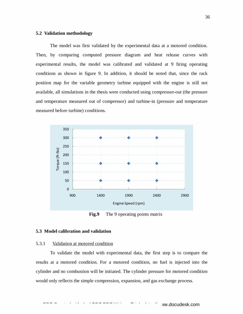
5.2 Validation methodology ................................................................................ 36
5.3 Model calibration and validation .................................................................. 36
5.3.1 Validation at motored condition ...................................................... 36
5.3.2 Model validation for firing cases ................................................... 37
5.4 Results for parametric study ......................................................................... 45
5.4.1 Injection timing variation ................................................................ 46
5.4.2 Injection pressure variation .............................................................. 50
5.4.3 Load/speed variation ......................................................................... 53
5.4.4 EGR level variation ......................................................................... 58
5.4.5 Compression ratio variation ............................................................. 60
5.5 Numerical study focusing on NOx emission ................................................ 63
5.5.1 Sensitivity of NOx prediction on major parameters .................... 63
5.5.2 Numerical study of five NOx kinetics .......................................... 64
6. CONCLUSIONS AND RECOMMENDATIONS .................................................. 68
REFERENCES .............................................................................................................. 71
APPENDIX I PROPERTIES OF BIODIESEL AND DIESEL FUEL ........................ 74
APPENDIX II DISCHARGE COEFFICIENTS WITH LIFT .................................... 79
APPENDIX III MODEL VALIDATION FOR BIODIESEL FUEL ........................... 81
VITA............... ............................................................................................................... 86

viii
LIST OF FIGURES
Page
Figure 1 Discretization of pipes in GT-Power ........................................................ 12
Figure 2 Engine cylinder modeling ........................................................................ 14
Figure 3 Intake and exhaust valve lift profile ......................................................... 15
Figure 4 Flow regions appropriate for typical bowl-in-piston
diesel engine geometries .......................................................................... 16
Figure 5 Injected mass is divided into many zones ................................................ 20
Figure 6 Numbering rule of the zones .................................................................... 21
Figure 7 Compressor maps ..................................................................................... 32
Figure 8 Turbine maps ............................................................................................ 32
Figure 9 The 9 operating points matrix .................................................................. 36
Figure 10 Model validation at the motored condition @ 1400 rpm ......................... 37
Figure 11 Engine performance comparison of simulation
and measurement ..................................................................................... 38
Figure 12 Difference of engine performance between simulation
and measurement ..................................................................................... 39
Figure 13 Pressure diagram comparison @ 1400 rpm 50 ft-lbs ............................... 40
Figure 14 Heat release curve comparison @ 1400 rpm 50 ft-lbs ............................. 40
Figure 15 Pressure diagram comparison @ 1400 rpm 150 ft-lbs ............................. 40
Figure 16 Heat release curve comparison @ 1400 rpm 150 ft-lbs ........................... 40

ix
Page
Figure 17 Pressure diagram comparison @ 1400 rpm 300 ft-lbs ............................. 41
Figure 18 Heat release curve comparison @ 1400 rpm 300 ft-lbs ........................... 41
Figure 19 Pressure diagram comparison @ 1900 rpm 50 ft-lbs ............................... 42
Figure 20 Heat release curve comparison @ 1900 rpm 50 ft-lbs ............................. 42
Figure 21 Pressure diagram comparison @ 1900 rpm 150 ft-lbs ............................. 43
Figure 22 Heat release curve comparison @ 1900 rpm 150 ft-lbs ........................... 43
Figure 23 Pressure diagram comparison @ 1900 rpm 300 ft-lbs ............................. 43
Figure 24 Heat release curve comparison @ 1900 rpm 300 ft-lbs ........................... 43
Figure 25 Pressure diagram comparison @ 2400 rpm 50 ft-lbs ............................... 44
Figure 26 Heat release curve comparison @ 2400 rpm 50 ft-lbs ............................. 44
Figure 27 Pressure diagram comparison @ 2400 rpm 150 ft-lbs ............................. 44
Figure 28 Heat release curve comparison @ 2400 rpm 150 ft-lbs ........................... 44
Figure 29 Pressure diagram comparison @ 2400 rpm 300 ft-lbs ............................. 45
Figure 30 Heat release curve comparison @ 2400 rpm 300 ft-lbs ........................... 45
Figure 31 Pressure diagram for different injection timing, diesel case .................... 47
Figure 32 Pressure diagram for different injection timing, biodiesel case ............... 48
Figure 33 Ignition delay for different injection timings ........................................... 49
Figure 34 Brake specific fuel consumption for different injection timings ............. 49
Figure 35 Indicated specific NO2 for different injection timings ............................. 49
Figure 36 Pressure diagram for different injection pressure, diesel case ................. 51

x
Page
Figure 37 Pressure diagram for different injection pressure, biodiesel case ............ 51
Figure 38 Ignition delay for different injection pressure .......................................... 52
Figure 39 bsfc for different injection pressure ......................................................... 52
Figure 40 Indicated specific NO2 for different injection pressure ........................... 53
Figure 41 Ignition delay for different load and speed .............................................. 54
Figure 42 Brake specific fuel consumption for different load and speed ................. 55
Figure 43 EGR level applied at each operating condition for
reference diesel case ................................................................................ 56
Figure 44 EGR level applied at each operating condition
for biodiesel case ...................................................................................... 56
Figure 45 Indicated specific NO2 for different load and speeds .............................. 57
Figure 46 Pressure diagram for different EGR level, diesel case............................. 58
Figure 47 Pressure diagram for different EGR level, biodiesel case ....................... 58
Figure 48 Ignition delay for different EGR level ..................................................... 59
Figure 49 Brake specific fuel consumption for different EGR level ........................ 59
Figure 50 Indicated specific NO2 for different EGR level ...................................... 59
Figure 51 Pressure diagram for different compression ratio
for diesel case ........................................................................................... 60
Figure 52 Pressure diagram for different compression ratio
for biodiesel case ...................................................................................... 61
Figure 53 Ignition delay for different compression ratio ......................................... 61
Figure 54 bsfc for different compression ratio ......................................................... 61

xi
Page
Figure 55 Indicated specific NO2 for different compression ratio ........................... 62
Figure 56 The approximation of M&B kinetics in GT-Power ................................. 66
Figure 57 The approximations of H&B and D&B kinetics in GT-Power ................ 66
Figure 58 Comparison of NO calculation with different
NO kinetics, diesel case ........................................................................... 66
Figure 59 Comparison of NO calculation with different
NO kinetics, biodiesel case ...................................................................... 67
Figure 60 Discharge coefficients against L/D ratio
for intake and exhaust valves ................................................................... 80
Figure 61 Pressure diagram comparison @ 1400 rpm 50 ft-lbs
for biodiesel case ...................................................................................... 81
Figure 62 Heat release curve comparison @ 1400 rpm 50 ft-lbs
for biodiesel case ...................................................................................... 81
Figure 63 Pressure diagram comparison @ 1400 rpm 150 ft-lbs
for biodiesel case ...................................................................................... 81
Figure 64 Heat release curve comparison @ 1400 rpm 150 ft-lbs
for biodiesel case ...................................................................................... 81
Figure 65 Pressure diagram comparison @ 1400 rpm 300 ft-lbs
for biodiesel case ...................................................................................... 82
Figure 66 Heat release curve comparison @ 1400 rpm 300 ft-lbs
for biodiesel case ...................................................................................... 82
Figure 67 Pressure diagram comparison @ 1900 rpm 50 ft-lbs
for biodiesel case ...................................................................................... 82
Figure 68 Heat release curve comparison @ 1900 rpm 50 ft-lbs
for biodiesel case ...................................................................................... 82

xii
Page
Figure 69 Pressure diagram comparison @ 1900 rpm 150 ft-lbs
for biodiesel case ...................................................................................... 83
Figure 70 Heat release curve comparison @ 1900 rpm 150 ft-lbs
for biodiesel case ...................................................................................... 83
Figure 71 Pressure diagram comparison @ 1900 rpm 300 ft-lbs
for biodiesel case ...................................................................................... 83
Figure 72 Heat release curve comparison @ 1900 rpm 300 ft-lbs
for biodiesel case ...................................................................................... 83
Figure 73 Pressure diagram comparison @ 2400 rpm 50 ft-lbs
for biodiesel case ...................................................................................... 84
Figure 74 Heat release curve comparison @ 2400 rpm 50 ft-lbs
for biodiesel case ...................................................................................... 84
Figure 75 Pressure diagram comparison @ 2400 rpm 150 ft-lbs
for biodiesel case ...................................................................................... 84
Figure 76 Heat release curve comparison @ 2400 rpm 150 ft-lbs
for biodiesel case ...................................................................................... 84
Figure 77 Pressure diagram comparison @ 2400 rpm 300 ft-lbs
for biodiesel case ...................................................................................... 85
Figure 78 Heat release curve comparison @ 2400 rpm 300 ft-lbs
for biodiesel case ...................................................................................... 85

xiii
LIST OF TABLES
Page
Table 1 Summary of alternative fuels candidates ................................................. 2
Table 2 Soot kinetics and the corresponding rate constants ................................. 31
Table 3 Effectiveness of the intercooler................................................................ 34
Table 4 Engine specification ................................................................................. 35
Table 5 Structure of the parametric studies .......................................................... 46
Table 6 How adjustable parameters affect the NOx calculation ........................... 64
Table 7 The NOx kinetics studied and their realization in GT-Power .................. 65
Table 8 Properties comparison between diesel 2 and biodiesel ............................ 74
Table 9 Enthalpy constants for vapor diesel and biodiesel ................................... 75
Table 10 Viscosities and thermal conductivities of diesel vapor ............................ 75
Table 11 Viscosities and thermal conductivities of biodiesel vapor ....................... 75
Table 12 Enthalpy constants for liquid diesel and biodiesel ................................... 76
Table 13 Viscosities and thermal conductivities of liquid diesel ............................ 77
Table 14 Viscosities and thermal conductivities of liquid biodiesel ....................... 77
Table 15 Intake valve flow coefficients .................................................................. 79
Table 16 Exhaust valve flow coefficients ............................................................... 79

1
1. INTRODUCTION
Compression ignition, direct injection engines (e.g. diesel engine) have dominated
the field of heavy-duty vehicles and marine transportations for a long time, and are
increasingly being applied in light-duty vehicles in the past 30 years. Compared to the
spark ignition engine (e.g. gasoline engine), the diesel engine has considerably higher
thermal efficiency due to its lean combustion, with a higher compression ratio, and lack of
throttle. However, the major fuel source for diesel engine, the petroleum based fuel, is
depleting at a very rapid rate. Of the 102 quadrillion Btu’s energy consumed in 2007 in
the United States, 39% was from petroleum based fuels and 69% of that was consumed in
transportation sector [1]. The depletion of petroleum fuel and its increasing cost have
raised much interest in looking for the alternate fuel for diesel engines.
Tremendous effort to search for alternative fuels has been made in the past several
decades, numerous alternative fuels have been studied and tested, including hydrogen,
coal, dimethyl ether (DME), biodiesel, etc. However, due to several certain established
end-use requirements, such as availability, supply, safety, cost-efficiency, etc., only a few
candidates remain active for testing and research. Major candidates and their main
advantages and disadvantages are summarized in table 1 (see next page).
Equation Chapter 1 Section 1
____________
This thesis follows the style of Journal of Automobile Engineering.

2
Table 1 Summary of alternative fuels candidates
Candidates Advantages Disadvantages
Hydrogen
High lower heating value.
“Zero” pollutant by emission.
Potentially renewable energy
source.
Refilling problem.
Safety issue due to high pressure
tank.
DME Less PM & NOx emission.
High cetane number.
Worse lubrication than diesel.
Safety issue due to high pressure
tank.
Coal Large accessible reserve. Injection problem.
Lubrication contamination.
Biodiesel
Low HC and CO emission.
Potentially renewable energy
source.
Low energy content.
Uncertain effect on NOx.
1.1 Biodiesel as an alternative fuel
In the past several decades, it has been found that biodiesel (esters derived from
vegetable oils) is a very promising one. The most common blend is a mix of 20% biodiesel
and 80% petroleum diesel, called “B20”. The widespread use of biodiesel is based on the
following advantages [2]:
Biodiesel is potentially renewable and non-petroleum-based
Biodiesel combustion produce less greenhouse gases
Biodiesel is less toxic and biodegradable
Biodiesel can reduce tailpipe emissions of PM, CO, HC, air toxics, etc
Little modifications are needed for the traditional CI engine to burn biodiesel
Biodiesel also has some negative attributes [2]:
Lower heating value, higher viscosity
Lower storage stability, material compatibility issue
Slightly higher NOx emission

3
Among the above attributes of biodiesel, the higher NOx emissions from biodiesel
fueled engines are a major concern due to more and restrict regulations, and therefore it
serves as the major motivation of this work.
1.2 Use of the engine cycle simulation to study a biodiesel fueled engine
In modern engine research and study, using hardware experiments alone would be
very expensive and time-consuming, and many cause and effect relationships implicit in
the test results are often hard to interpret. On the other hand, modeling and simulation
approaches, although less precise in predicting the outcome of a specific test, could
effectively isolate one variable at a time and conduct parametric studies on it. Therefore
simulation could point out cause-effect relationships more clearly, and a validated model
could be a very useful tool to study new type of engines or engines running with new type
of fuels. Since people still don’t have a very clear understanding on the effect of using
biodiesel on a diesel engine, together with experimental study, a simulation study of the
biodiesel engine is necessary.
Engine cycle simulation models could be divided into three major categories:
zero-dimensional models, quasi-dimensional, multi-zone models and multi-dimensional
models. Zero-dimensional models have been successfully used to predict engine
performance and fuel economy, but they are too simplified to predict the engine emission
accurately. On the other hand, though multi-dimensional models could provide the most
accurate prediction due to more detailed geometry modeling, the significantly increased
computation time becomes a major limiting factor of applying multi-dimensional models.
Among them, quasi-dimensional, multi-zone models could be effectively used as an engine
development tool because they combine some of the advantages of zero-dimensional and
multi-dimensional models. Therefore, quasi-dimensional, multi-zone model would be a
good choice for this biodiesel engine study.

4
2. OBJECTIVES AND MOTIVATIONS
The major objective of this project is to use an engine cycle simulation to study a
biodiesel fueled engine focusing on the engine overall performance and emission
characteristics. To achieve this objective, several specific tasks need to be done:
Equation Section (Next)
1. First of all, by using the engine simulation software ‘GT-Power’, build a biodiesel fueled
engine model which is corresponding to the real engine. The model should have submodels
which reflect all the features in the real engine, including direct injection, EGR,
turbocharging, charged air intercooling, EGR intercooling, and etc. The model would be
quasi-dimensional and multi-zonal, and be able to predict engine performance and
emissions (e.g. NOx concentration, PM) at different operating conditions.
2. After constructing the model, the second task is to calibrate the model with experimental
data at several typical operating conditions (e.g. low speed low load, high speed high load).
The major calibration objective is to match the computed pressure diagram and heat release
rate diagram with the experimental ones. Before calibration, parametric studies on major
adjustable parameters are needed to determine their sensitivity on pressure diagram and
other major parameters such as ignition delay, fuel consumption, and etc.. After
calibration, the difference between simulation and measurement for main parameters
should be lower than 10%.
3. Using the calibrated model, study the effect of various parameters on engine
performance and emission for both biodiesel and reference diesel case. By comparing and
analyzing the results, look for the cause of changes in performance and emission due to
biodiesel combustion in diesel engine.

5
3. LITERATURE REVIEW
A review of recent biodiesel fueled engine research activities is presented here.
Activities can be roughly divided into two aspects: engine experimental studies and
numerical studies. Both of these types of studies focus on the performance and emission
characteristics of biodiesel fueled engines and comparison to the conventional diesel
engine.
Equation Section (Next)
3.1 Previous experiment studies
3.1.1 Effect of injection timings
In many papers reviewed, the start of injection(SOI) for biodiesel is advanced
than those for conventional diesel engine. As an example, for the experiment done by [3],
an earlier start of injection for neat biodiesel fuels was found. The biodiesel fuel injected
about 2.3º earlier than diesel no.2, and the B20 (blend of 20% biodiesel and 80% diesel)
were 0.25º-0.75º earlier than diesel no.2. According to [4, 5], the SOI are majorly affected
by changes in three physical properties: density, bulk modulus of compressibility, and
speed of sound. Because of the higher bulk modulus of compressibility and speed of
sound for biodiesel, there is a more rapid transfer of the fuel pump pressure wave to the
injector needle, resulting in earlier needle lift and effectively a little advance in injection
timing. However, this effect only exists in rotary/distributor-style fuel injection pumps,
and not in common-rail fuel injection systems.
In terms of NOx emission, advanced injection timing is considered by many
authors as a major reason for change in NOx emission for biodiesel engine [3, 5, 6]. In
the experimental study conducted by [7], tests were done with a Yanmar L70 EE
air-cooled, four-stroke, single cylinder DI diesel engine with a maximum power output of
5.8 horsepower, operating at high load and low load. The fuels include BP325 (baseline

6
petroleum diesel fuel with 325 ppm sulfur), B20, B40, B100, Fischer-Tropsch (FT) diesel
and its blend with BP325. The results showed that brake specific NOx emissions decrease
with retarded injection timing at all loads. At high load, all the fuels demonstrate roughly
the same NOx emissions as a function of fuel injection timing. This observation indicates
that for these fuels the engine-out NOx emission differences are related to shifts in SOI
timings.
3.1.2 Effect of ignition delay
Most of the studies observed that ignition delay for biodiesel is shorter than that
of conventional diesel [8, 9, 10, 11]. Eckerle [8] did experiments with a Cummins ISB
6.7L six cylinder engine with Bosch CRIN 3.0 HPCR fuel system. In these studies only
one of the six cylinders is active and the others are unfired. The study investigated four
fuels: Low Cetane Diesel, Low Cetane B20 Blend, High Cetane Diesel, and High Cetane
B20 Blend. Results showed that at 1700 rpm low load condition, ignition delay for High
and Low Cetane B20 are shorter than High and Low Cetane Diesel, respectively. The
difference is 3º for Low Cetane case and 0.5º for High Cetane case.
The decrease of ignition delay varies with different biodiesel feedstock. Some
studies [12] found that ignition delay of CME (coconut oil methyl ester) is shorter than
RME (rapeseed oil methyl ester) but longer than PME (palm oil methyl ester). The
decrease of ignition delay also varies with engine operating conditions, i.e. engine speed
and load. Experiments done by [5] indicated that compared with diesel fuel, ignition
delay at 1300 rpm with B20 decreased by 5% at low load and 10% at high load , and at
75% load B20 decreased by 6.9% at load speed and 17.2% at high speed condition.
Higher cetane number of biodiesel is generally considered as indication of its shorter
ignition delay. Analysis in [8] indicated that ignition delay is affected by aromatic
hydrocarbon content and is generally characterized by cetane number.

7
In terms of NOx emissions, ignition delay is also considered by some
investigators [5, 7, 8] to be an important part of the NOx emission difference between
diesel and biodiesel. According to [8], at light load, the relatively longer ignition delay
for diesel fuel allow most or all of the fuel to be injected before combustion begins. This
pre-mixing results in a more dilute combustion zone and in lower peak combustion
temperatures. This in turn results in lower NOx formation in diesel engine compared with
biodiesel engine. But [8] also indicated that at high load conditions where the combustion
is dominated by a diffusion flame, the ignition delay effect is weak and there is only a
small net combustion impact associated with burning biodiesel. The difference in NOx
between either diesel fuel and its B20 blend is considerably less than the difference in
NOx between the two commercial diesel fuels.
3.1.3 Effect of flame temperature and soot radiation
A lot of investigators [8, 9, 13, 14] hold that engines fueled with biodiesel have
higher flame temperature than conventional diesel engines and the higher flame
temperature is one of the major reasons for increased NOx emission from biodiesel
engine. Results from [8] shows that the higher aromatic content in biodiesel produces
higher flame temperatures and therefore higher NOx emissions. The author also indicated
that this effect is most significant for modes of combustion dominated by diffusion
burning, as is characteristic of higher load engine operation. In addition, the methyl ester
compounds in the biodiesel have more double bonds than the base diesel fuel and these
double bonds have the effect of increasing the flame temperature [13]. From a
macroscopic point of view, advanced injection timing and shorter ignition delay produce
a higher flame temperature during the diffusion burning period [9]. Also, for improved
combustion the temperature in the combustion chamber can be expected to be higher
[14].

8
Recent studies have shown that radiative heat transfer from soot could
significantly affect the NOx formation during combustion [15, 16]. Some investigators
have reported that the “cooling effect” of soot radiation may reduce NOx emission by
approximately 25% [15]. Radiation from soot produced in the flame zone is a major
source of heat transfer away from the flame, and can lower bulk flame temperature by 25
K to 125 K, depending on the amount of soot produced at the engine operating conditions.
Such reductions in the flame temperature would accordingly decrease the NOx by the
thermal mechanism by 12% to 50%. Thus, an in-cylinder soot-NOx tradeoff exists in
diesel engines and this tradeoff appears to fit biodiesel emission data well [13]. As stated
previously, biodiesel fuels in general produce less soot than petroleum diesel fuel, which
is likely a consequence of the fuel bound oxygen. This reduction in soot would
theoretically reduce the “cooling effect” via soot radiative heat transfer, and thus leave
NOx formation unsuppressed. Also, soot radiation may explain the variation in NOx
emissions between the different esters of which biodiesel consists [13].
3.2 Previous simulation studies
Due to the subtlety and complexity of comparing biodiesel and diesel combustion
in direct injection engines, numerical studies (engine simulations) have been applied in
addition to experimental studies.
The numerical study in [13] applied a so-called well-mixed balloon model to
investigate the flame temperature and NOx formation of biodiesel combustion.
Calculation were made using Cantera in a MATLAB environment. The well-mixed
balloon is a model that simulates the time history of a jet of fuel into a combustion
chamber containing oxidizer. In the well-mixed balloon, the mass output is zero and thus
the balloon grows as mass flows in. In time the balloon grows and the fuel-air mixture in
the balloon reaches the ignition conditions and then ignites. This leads to a sudden
increase in temperature [13]. Two fuels, methyl butanoate and methyl trans-2-butenoate,
9
were simulated, and the results showed that the double bonded methyl trans-2-butaneoate
gave a 14 K higher flame temperature than the other fuel. The investigator believed that
this change in temperature caused an increase in NOx emissions of 159 ppm [13]. Also,
the author did the model sensitivity analysis on the influence of the various NOx
mechanisms. Results revealed that the thermal NOx mechanism had the most visible
contribution to the NOx formation (92%), comparing to other mechanisms such as N2O
mechanism (1%) and Fenimore mechanism (13%) [13].
Due to the over-simplicity of zero-dimensional model, and the long computational
time of three-dimensional model, quasi-dimensional multi-zone models are increasingly
applied by many investigators [17, 18, 19, 20]. The study in [17] developed a
quasi-dimensional, multi-zone, direct injection (DI) diesel combustion model. The model
was implemented in a full cycle simulation of a turbocharged engine. The combustion
model accounted for transient fuel spray evolution, fuel-air mixing, ignition, combustion
and NO and soot pollutant formation. The results demonstrated that the model can predict
the rate of heat release and engine performance with high fidelity, while more effort is
needed to enhance the fidelity of emission prediction. Arsie et al. [18] reported that the
model they developed successfully predicted engine performance and emissions. In
addition, the constants in their submodels remained the same throughout the engine
operating range, which enabled this quasi-dimensional multi-zone model to be used for
prediction purposes. By using the GT-Power software, [20] also developed a multi-zone
model to analyze the performance and emissions of different types of diesel and biodiesel
fuels. The model was calibrated at a default case using normalized burn rate and it was
then used to predict pressure diagram, heat release and NOx emissions for soybean based
biodiesel, rapeseed based biodiesel and reference diesel. The results showed that three
fuels gave almost the same pressure diagram, while the two biodiesel cases gave slightly
higher heat release rate than that of diesel case. At two load conditions, results showed 60%
higher NOx concentration from the two biodiesels fuel than that of diesel fuel. Since the

10
model has not been well calibrated at all engine operating conditions, these results could
be very preliminary.
To obtain more detailed combustion insight, 3D simulation is still applied by
some investigators. In [8], a KIVA model was developed and calibrated using the engine
data for diesel no.2 and B100 biodiesel. Good agreement between measured and
predicted heat release is obtained with some discrepancies associated with the start of
combustion. In terms of emissions, the author compared soot vs. NOx tradeoff between
measurement and prediction and the agreement is also quite good. After completing the
KIVA model validation, a detailed examination of the impact of engine controls settings
on NOx formation due to the lower energy content of the B20 blends was conducted. Two
test cycles (UDDS6K and HWY55) were conducted by the KIVA model. Final results
showed that at higher speeds and loads, the change in engine control settings due to the
lower energy content of the blended fuel led to a NOx increase on the order of 3-4%. The
author believed that this accounts for the majority of the NOx difference between a B20
blend and its base diesel fuel.

11
4. MODELING DI ENGINE IN GT-POWER
4.1 Overview
GT-Power is a popular engine simulation tool which is designed for steady-state
and transient simulations. It is applicable to many types of internal combustion engines and
provides the user with many components to model any advanced concept.
GT-Power is based on one-dimensional gas dynamics, representing the flow and
heat transfer in pipes and other components of an engine system. In addition, many other
specialized models (e.g. emission production model, T/C model) can be applied for many
kinds of system analysis. The detailed model information related to the present work is
described in the following sections.
Equation Section (Next)
4.2 Modeling fluid properties
In GT-Power, a gas reference object is commonly described by its C:H:O:N
composition, lower heat value, critical temperature and pressure, enthalpy, and transport
properties which includes viscosity and thermal conductivity.
For liquids, information about enthalpy, density, and transport properties are the
necessary input to GT-Power. In addition, typically every liquid reference object must be
associated with a gas reference object so that the properties of the liquid will be known if
the fluid evaporates.
The detailed properties of the biodiesel and reference diesel that are used in the
simulation is listed in Appendix I.

12
4.3 Modeling fluid flow in pipes
4.3.1 General governing equations
In GT-Power, the fluid flow in pipes is simplified as a transient, one-dimensional
problem, which involves the simultaneous solution of continuity, momentum and energy
equations only in flow direction. All quantities are averages across the flow direction since
it’s a one-dimensional problem.
The whole system is discretized into many volumes, where each flowsplit is
represented by a single volume, and every pipe is divided into one or more volumes, see
figure 1 [21].
Fig.1 Discretization of pipes in GT-Power
The continuity, momentum and energy equations being solved are [21],
boundries
dmm
dt (4-1)
( )( ) ( )s fluid wall
boundries
d me dVp mH hA T T
dt dt (4-2)
1( ) 4
2 2f p
boundries
u u dxAdpA mu C C u u A
dm D
dt dx
(4-3)

13
4.3.2 Friction loss and surface roughness effect
Pressure loss in pipes due to friction is obtained from by several common
correlations, using the Reynolds number and the surface roughness.
For smooth surface [21],
D
D0.25
16 in laminar region, Re 2000
Re
0.08 in turbulent region, Re >4000
Re
f
D
f
D
C
C
(4-4)
For rough surface and turbulent flow [21],
, 20.25
0.08 0.25max ,
Re2log 1.74
2
f rough
D
CD
h
(4-5)
4.3.3 Heat loss and surface roughness effect
The heat transfer from the fluid to the pipe wall is calculated by correlated heat
transfer coefficient. For smooth pipes [21],
2/31
Pr2
g f eff ph C U C (4-6)
For rough surface [21],
,
,
n
f rough
g rough g
f
Ch h
C
(4-7)
where 0.2150.68 Prn
,g roughh = heat transfer coefficient of rough pipe
,f roughC = friction coefficient of rough pipe

14
4.4 Modeling cylinder, cylinder valves and ports
To model the cylinder geometry, the bore, stroke, connecting rod length, wrist pin
to crank offset, compression ratio, and TDC clearance height are inputted into the program,
as shown in figure 2 [21]. The detailed values for the cylinder geometry are consistent with
the engine specifications from the engine manufacturer. The one exception was the
compression ratio which was determined from manual measurement of the clearance
volume and the displacement volume. Values used in the simulation are listed in the engine
specifications which is described in the next section.
Fig.2 Engine cylinder modeling [21]
For valves, the simulation uses a valve lift profile, nominal flow area, and discharge
coefficient to describe the cylinder valves. The flow rate is calculated by the following
equations [21]:
1/
0eff is is D R r ism A U C A P U
(4-8)
In the equation, DC refers to the discharge coefficient which is provided by the

15
engine manufacturer, and RA refers to the reference area of the cylinder valves, which is
calculated by the relation:
R refA D L (4-9)
where refD is the reference diameter of the valve and L is the valve lift for a certain
valve lift position. RA and DC are unique for each lift position. Figure 3 shows the
intake/exhaust valve lift profile, and the detailed discharge coefficients with valve lift can
be found in Appendix II.
Fig.3 Intake and exhaust valve lift profile
The intake and exhaust ports into an engine’s cylinder are modeled geometrically
with pipes. According to the simulation, the flow coefficients of the valves include the flow
losses caused by the port, so the friction and pressure loss for the intake and exhaust ports
are set to zero in the model. For convenience, the wall temperature for the intake and
exhaust ports are approximated to as 450 K and 550 K, respectively.
0
2
4
6
8
10
12
0 90 180 270 360 450 540 630 720
Val
ve L
ift
(mm
)
Crank Angle (deg)
Exhaust Valve Intake Valve
TDC

16
4.5 Modeling in-cylinder flow and heat transfer
4.5.1 In-cylinder flow model
The in-cylinder flow model breaks the cylinder into four regions: the squish region
(I), head region (II), center region (III), and piston cup region (IV), as shown in figure 4
below.
Fig.4 Flow regions appropriate for typical bowl-in-piston diesel engine geometries
At each time step in each region, the mean radial velocity, axial velocity, and swirl
velocity are calculated taking into account the cylinder geometry, the piston motion, and
flow rate/swirl/tumble of the incoming and exiting gases through valves. The flow model
also includes single zone turbulence model which solves the turbulence kinetic energy
equation and the turbulence dissipation rate equation. The resultant turbulence intensity
and in-cylinder velocity are used in the combustion simulation and heat transfer
calculation.
According to the data from engine manufacturer, swirl and tumble coefficients for
the intake valves are specified versus L/D (lift over diameter), and these values are used to
determine the swirl and tumble torque by the following equation. Swirl and tumble torque
will be applied to the in-cylinder gases and therefore affect the in-cylinder flow solution.
squish region center region
piston cup region
head region

17
2 s
is
TSwirl Coefficient
m U D
(4-10)
t
is
TTumble Coefficient
m U D
(4-11)
121
0
21
1is rU RT P
(4-12)
where: sT = swirl torque
tT = tumble torque
m = mass flow rate
isU = isentropic valve velocity
D = cylinder bore
rP = absolute pressure ratio
R = gas constant
0T = upstream stagnation temperature
= specific heat ratio
4.5.2 In-cylinder heat transfer model
(1) Woschni model
The in-cylinder heat transfer applied in the engine model is basically the Woschni
model [22] which is described as follows.
Re
m
p mcv Bh B
Nu C Ck
(4-13)
where 0.75 0.62, , , , and 0.035p
pk T T v w C
RT

18
1 0.75 1.62m m m m
ch CB p w T (4-14)
where the local average gas velocity w is correlated as follows,
1 2
d rp m
r r
V Tw C v C p p
p V
(4-15)
where Vd is the displaced volume;
p is the instantaneous cylinder pressure;
pr, Vr, Tr are the pressure, volume and temperature at the reference state;
pm is the motored cylinder pressure at the same crank angle as P.
For the gas exchange period: C1=6.18, C2=0
For the compression period: C1=2.28, C2=0
For the combustion and expansion period: C1=2.28, C2=3.24×10⁻³
Woschni’s correlation, with the exponent m equal to 0.8, can be summarized as:
0.2 0.8 0.8 0.553.26c convh C B p w T
(4-16)
where Cconv is the multiplier for convection heat transfer (def = 1.0)
(2) Hohenberg model
Based on the basic form of Woschni equation,
0.2 0.8 0.8 0.553.26c convh C B p w T
(4-17)
An attempt was made to give improved definitions of the individual terms used in
the above equation for the heat transfer coefficient by Hohenberg in 1979 [23].
The term, 0.2D , makes allowance for the cylinder bore effect on the flow near
the wall. However, since the cylinder volume VC in IC engine changes periodically,
Hohenberg applied the diameter D of a ball as a characteristic quantity where its volume
corresponds to the momentary cylinder volume VC:

19
3
6C
DV
(4-18)
0.33
CD C V (4-19)
Hence,
0.20.2 0.066
CD D C V
(4-20)
In order to compensate the variations in radiation which is known to increase with
increasing diameters, the final form of this term become,
0.2 0.06
CD C V (4-21)
The term, 0.8 0.53p T , indicates that the heat transfer coefficient increases with
rising 0.5T pressure and decreases with rising temperatures. After systematic tests with
either varying pressure or varying temperature, it has been found out that the effect of
temperature and pressure alone can be suitably defined by the following,
0.6 0.5p T
(4-22)
The term, 0.8v , describes the effect of flow velocity on heat transfer. However,
the velocity is subjected to periodical changes so that the customary use of the mean piston
speed only supplies information on the rise in the velocity level with increasing speed but
not on the variations with crankshaft angle. The following points are relevant for the
formulation of an equation to describe actual conditions: the intake swirl, turbulence
caused by intake swirl, super-imposed flow, and turbulence caused by combustion. To
approximate the above effect, the original term has been modified as follows,
0.8
0.8 0.2 0.1
2pv p T v C (4-23)
The time-relation is described by 0.2 0.1p T , the mean piston speed pv makes
compensation for the rise in the velocity with increasing engine speed, and the constant 2C

20
for combustion turbulence and the relatively small radiation portion.
By summarizing the above equations, the heat transfer coefficient can be defined
by the following expression (4-24):
0.8
0.06 0.8 0.4
1 2pCh C V p T v C (4-24)
where
h - heat transfer coefficient [W/m2-K]
VC - cylinder volume [m3]
p - in-cylinder pressure [bar]
T - in-cylinder temperature [K]
pv - mean piston speed [m/s]
C1, C2 - constants (typical values are C1=130 and C2=1.4)
4.6 Modeling combustion and emission formation
The combustion model (DI-Jet Model) is a quasi-dimensional multi-zone
combustion model for direct injection compression ignition engine. It is primarily used to
predict burn rate and NOx emissions. Soot is also predicted, but the predicted
concentrations are not particularly meaningful and should be used to study only trends in
the results.
Fig.5 Injected mass is divided into many zones

21
Fig.6 Numbering rule of the zones
As shown in figure 5, the total injected mass is divided into zones: 5 radial zones
and a maximum of 80 axial zones (depending on the value specified in the
'EngCylCombDIJet' model) [21]. Figure 6 shows how the zones are numbered. At each
timestep taken by the code during the injection period, an axial “slice” (five radial zones) is
injected into the cylinder (if the time steps are very small, the fuel may be injected at only
every other timestep). The total mass of fuel in all of the zones will be equal to the specified
injection rate (mg/stroke) divided by the specified number of nozzle holes. (The DI-Jet
model really models the plume from only one nozzle hole.) The mass of fuel in each axial
“slice” is determined by the injection pressure at that timestep and the elapsed time since
the last zones were injected. This mass injected at each timestep is divided equally between
the five radial zones. The instantaneous injection pressure is also used to calculate the
injection velocity of each axial slice.
Each zone additionally contains subzones for liquid fuel, unburned vapor fuel and
entrained air, and burned gas. Immediately after a zone is injected, the zone is 100% liquid
fuel. As the zone moves into the cylinder, it “entrains” air and the fuel begins to evaporate,
thus forming the unburned subzone. The mass of the entrained air causes the velocity of the
zone to decrease because momentum of the zone is conserved. The outer zones entrain air
more quickly than the inner zones, thus decreasing their velocity more quickly and
resulting in less penetration distance as can be seen in figure 5.
From the mass of vapor fuel and entrained air in each unburned subzone, the zonal
fuel to air ratio is known. The zonal temperature is calculated taking into account the

22
temperature of the injected fuel, entrained air temperature, and the effects of the fuel
evaporation. When the combination of cylinder pressure, zonal temperature, and fuel-to-air
ratio becomes combustible, the fuel in the zone ignites, further changing the temperature
and composition. All products of combustion will be moved to the burned subzone. NOx
and soot are calculated independently in each burned subzone taking into account the
fuel/air ratio and temperature. The total cylinder NOx and soot are the integrated total of all
of the individual burned subzones.
4.6.1 Injection submodel
In the injection submodel, assume the flow through each nozzle is quasi-steady and
one-dimensional, the instantaneous fuel flow rate through the nozzle, 𝑚𝑖 , is given by the
following equation [21]:
2
fc
i n n fi i c
fi
m C A P P
(4-25)
where 𝐶𝑛 is the discharge coefficient;
𝐴𝑛 is the nozzle hole area;
𝜌𝑓𝑖 is the density of the fuel in the injector;
𝜌𝑓𝑐 is the density of the fuel in the cylinder;
𝑃𝑖 is the instantaneous injection pressure;
𝑃𝑐 is the instantaneous pressure in cylinder;
Since 𝑚𝑖 = 𝜌𝑓𝑖𝐴𝑛𝑈𝑖 the fuel injection velocity at the nozzle tip 𝑈𝑖 can be
calculated as:
2fc i c
i n
fi fi
P PU C
(4-26)
Also, the total injected fuel per event can be related by the following equation [21]:
_
_
inj end
total iinj start
tm m dt
t (4-27)

23
In the program, the injected mass of fuel per event, 𝑚𝑡𝑜𝑡𝑎𝑙 , and the injection
pressure profile are needed to be specified in the “injector” object. From the pressure
profile 𝑚𝑖 can be calculated by equation (4-25) left 𝐶𝑛 unknown. Then from equation
(4-27) and the specified 𝑚𝑡𝑜𝑡𝑎𝑙 , 𝐶𝑛 can be calculated. The reasonable range for 𝐶𝑛 is 0.6
to 0.8 and if the calculated 𝐶𝑛 is out of this range, there might be something wrong with
the pressure profile or specified 𝑚𝑡𝑜𝑡𝑎𝑙 value.
4.6.2 Fuel spray dynamics
(1) Fuel jet penetration
The fuel enters the combustion chamber with a nominal centerline velocity equal
to:
2fc i c
i n
fi fi
P PU C
(4-28)
where 𝐶𝑛 is the discharge coefficient of the nozzle;
𝜌𝑓𝑖 is the density of the fuel in the injector;
𝜌𝑓𝑐 is the density of the fuel in the cylinder;
𝑃𝑖 is the instantaneous injection pressure;
𝑃𝑐 is the instantaneous pressure in cylinder;
The breakup time and the penetration distance at the centerline are given by [21]:
7
br
0.5
br
1 0.06 for t<t
0.06 for t>t
i
br
i br br
tS U t
t
S U t t t
(4-29)
0.29 3
fc nnbr br
na i
DLt C
D U
(4-30)
where Ln/Dn is the aspect ratio of the nozzle;
Cbr is the breakup time multiplier (def = 1.0)
24
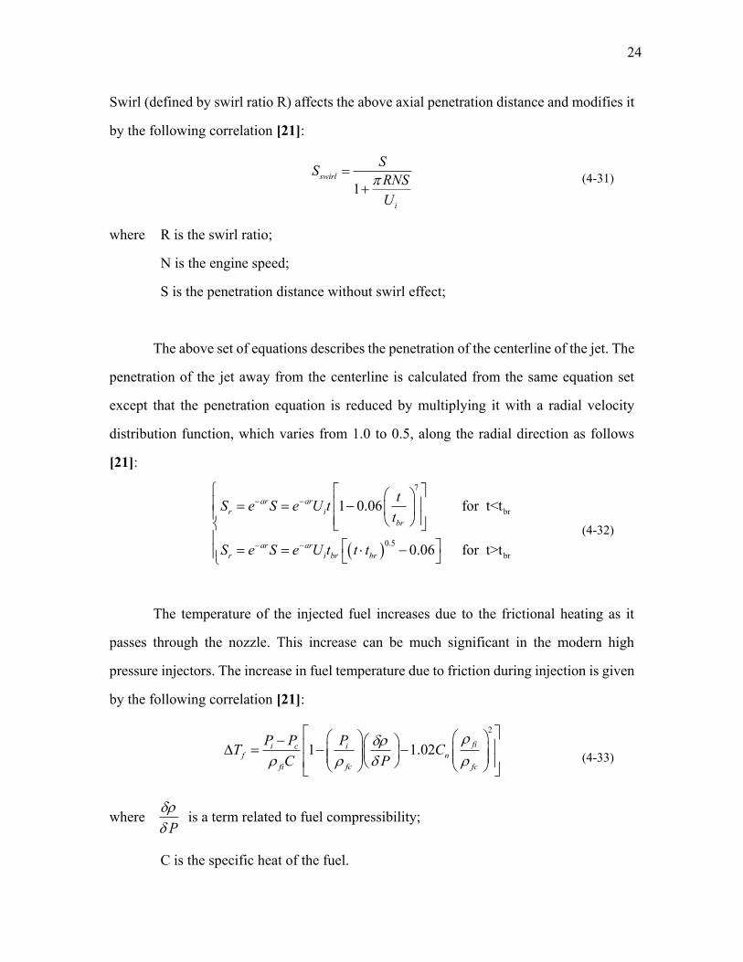
Swirl (defined by swirl ratio R) affects the above axial penetration distance and modifies it
by the following correlation [21]:
1
swirl
i
SS
RNS
U
(4-31)
where R is the swirl ratio;
N is the engine speed;
S is the penetration distance without swirl effect;
The above set of equations describes the penetration of the centerline of the jet. The
penetration of the jet away from the centerline is calculated from the same equation set
except that the penetration equation is reduced by multiplying it with a radial velocity
distribution function, which varies from 1.0 to 0.5, along the radial direction as follows
[21]:
7
br
0.5
br
1 0.06 for t<t
0.06 for t>t
ar ar
r i
br
ar ar
r i br br
tS e S e U t
t
S e S e U t t t
(4-32)
The temperature of the injected fuel increases due to the frictional heating as it
passes through the nozzle. This increase can be much significant in the modern high
pressure injectors. The increase in fuel temperature due to friction during injection is given
by the following correlation [21]:
2
1 1.02fii c i
f n
fi fc fc
P P PT C
C P
(4-33)
where P
is a term related to fuel compressibility;
C is the specific heat of the fuel.
25
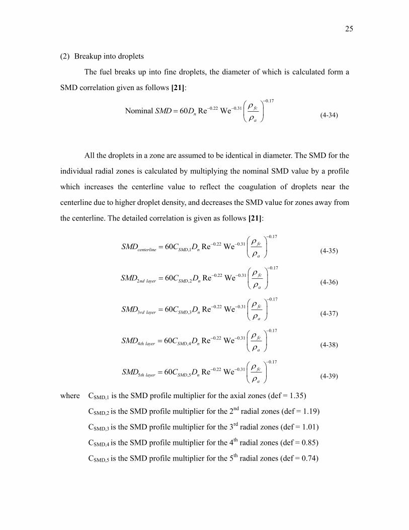
(2) Breakup into droplets
The fuel breaks up into fine droplets, the diameter of which is calculated form a
SMD correlation given as follows [21]:
0.17
0.22 0.31Nominal 60 Re Wefc
n
a
SMD D
(4-34)
All the droplets in a zone are assumed to be identical in diameter. The SMD for the
individual radial zones is calculated by multiplying the nominal SMD value by a profile
which increases the centerline value to reflect the coagulation of droplets near the
centerline due to higher droplet density, and decreases the SMD value for zones away from
the centerline. The detailed correlation is given as follows [21]:
0.17
0.22 0.31
,160 Re Wefc
centerline SMD n
a
SMD C D
(4-35)
0.17
0.22 0.31
2 ,260 Re Wefc
nd layer SMD n
a
SMD C D
(4-36)
0.17
0.22 0.31
3 ,360 Re Wefc
rd layer SMD n
a
SMD C D
(4-37)
0.17
0.22 0.31
4 ,460 Re Wefc
th layer SMD n
a
SMD C D
(4-38)
0.17
0.22 0.31
5 ,560 Re Wefc
th layer SMD n
a
SMD C D
(4-39)
where CSMD,1 is the SMD profile multiplier for the axial zones (def = 1.35)
CSMD,2 is the SMD profile multiplier for the 2nd
radial zones (def = 1.19)
CSMD,3 is the SMD profile multiplier for the 3rd
radial zones (def = 1.01)
CSMD,4 is the SMD profile multiplier for the 4th
radial zones (def = 0.85)
CSMD,5 is the SMD profile multiplier for the 5th
radial zones (def = 0.74)

26
(3) Air entrainment
As the jet develops, it entrains air and residuals from the initial charge of the
cylinder. The entrainment is nominally calculated from the conservation of the initial jet
momentum. The initial momentum of zone is calculated from the injection velocity (Ui)
and fuel mass (mf). The fuel zone decelerates according to the prescribed expression given
above. Using the principle of conservation of momentum, the total amount of air it
entrained (ma) at any instant can be calculated and conveniently expressed as a multiple of
the fuel mass in that zone [21]:
1i
a f
Um m
dSdt
(4-40)
The rate of air entrainment in any given time step can be calculated s a derivative of
the above expression. Before and after ignition, the rate of entrainment is respectively set
to:
1before ignition: a a
b
dm dmC
dt dt
(4-41)
1after ignition: a a
a
dm dmC
dt dt
(4-42)
where Cb is the entrainment multiplier before combustion (def = 1.2)
Where Ca is the entrainment multiplier after combustion (def = 0.5)
After jet impingement on the bowl surface, a wall jet is formed along the bowl
sidewall. The entrainment rate is further modified to account for the development of the
wall jet along the bowl surface:
2 1a a
w
dm dmC
dt dt
(4-43)
where Cw is the entrainment multiplier after wall impingement (def = 1.2)

27
(4) Evaporation of the droplets
Once the droplets have been injected, they begin to evaporate and their diameters
reduces gradually. The evaporation rate is strongly dependent on the relative velocity of the
droplet. It is assumed that the drag acting on the droplets reduces their speed rapidly
according to the following differential equation based on the Stokes drag law:
2
18 3d d d d
d d
U U U D
t D D t
(4-44)
The solution of the above equation yields an exponential decay function, with a
time constant proportional to Dd2/υ. Once the droplets have slowed down to the velocity of
the surrounding gas, the Sherwood number for evaporation rate and the Nusselt number for
convective heat transfer go to 2. The evaporation of the droplet can be diffusion-limited or
boiling-limited. In the diffusion-limited case, the evaporation rate per droplet is given by
[21]:
2vd
dmG D
dt
(4-45)
where 1
lnd
G ShD
1/3 1/2
d
1
Sh 2 0.57Sc Re
Re
Sc
is the mass diffusivity
D is the diameter of a droplet
o
d
Y Y
Y
UD
28
4.6.3 Ignition and combustion model
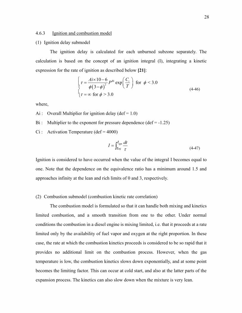
(1) Ignition delay submodel
The ignition delay is calculated for each unburned subzone separately. The
calculation is based on the concept of an ignition integral (I), integrating a kinetic
expression for the rate of ignition as described below [21]:
2
10 6exp for < 3.0
3
for > 3.0
Bi iCAiP
T
(4-46)
where,
Ai : Overall Multiplier for ignition delay (def = 1.0)
Bi : Multiplier to the exponent for pressure dependence (def = -1.25)
Ci : Activation Temperature (def = 4000)
ign
inj
t dtI
t (4-47)
Ignition is considered to have occurred when the value of the integral I becomes equal to
one. Note that the dependence on the equivalence ratio has a minimum around 1.5 and
approaches infinity at the lean and rich limits of 0 and 3, respectively.
(2) Combustion submodel (combustion kinetic rate correlation)
The combustion model is formulated so that it can handle both mixing and kinetics
limited combustion, and a smooth transition from one to the other. Under normal
conditions the combustion in a diesel engine is mixing limited, i.e. that it proceeds at a rate
limited only by the availability of fuel vapor and oxygen at the right proportion. In these
case, the rate at which the combustion kinetics proceeds is considered to be so rapid that it
provides no additional limit on the combustion process. However, when the gas
temperature is low, the combustion kinetics slows down exponentially, and at some point
becomes the limiting factor. This can occur at cold start, and also at the latter parts of the
expansion process. The kinetics can also slow down when the mixture is very lean.

29
For each zone, the kinetic rate of combustion in term of fuel consumption is
determined by equation (4-48) [21]:
2
3 . 0 e x p f o r 3 . 0
0 for 3.0
cBk cc
k
dm CA P
dt T
dm
dt
(4-48)
where mk is the burned mass of fuel in a specific zone
Ac is the overall combustion rate multiplier (def = 1.0)
Bc is the multiplier to the exponent for pressure dependence
Cc is the activation temperature for combustion kinetics
If the combustion is kinetically limited, the fuel is consumed at the rate dictated by
the above equation. In such a case, the mass of fuel calculated by equation (D-3) plus mass
of air proportional to the air/fuel ratio of the unburned subzone are transferred from a
unburned subzone to the corresponding burned subzone. If the combustion is mixing
controlled, i.e. the amount fuel available in the unburned subzone is less than the one
prescribed by equation (D-3), only the available fuel is burned. In both cases, however,
care is taken such that the burned subzone equivalence ratio never exceeds the carbon limit.
It should be noted that once the unburned zone is fully consumed, fuel energy may
continue to be released due to oxidation of burned subzone species as the burned subzone is
further diluted by the entrained air.
4.6.4 Submodels for emission formation
(1) Submodel for NOx prediction
As mentioned above, NOx is calculated independently in each burned subzone and
the total NOx emission is the summation of the NOx of each individual burned subzone. In
each burned subzone, NOx calculation is primarily based on the extended Zeldovich
mechanism. k1, k2, and k3 are the rate constants (from [24]) that are used to calculation the

30
reaction rates of the three equations below, respectively.
1
2 2N oxidation rate equation: O + N NO + Nk
(4-49)
2
2N oxidation rate equation: N + O NO + Ok
(4-50)
3OH reduction rate equation: N + OH NO + H
k
(4-51)
act-38000 C
10
1k = 7.60 10 eTb
(4-52)
-3150
6
2k = 6.40 10 eb
TbT (4-53)
10
3k = 4.10 10 (4-54)
where Tb is the temperature for burned subzone, and Cact is the multiplier for activation
temperature.
(2) Submodel for soot prediction
The submodel for soot prediction is based on two-step empirical soot model which
was established by Hiroyasu et al. in 1985 [25]. It considers the soot formation process as
involving two reaction steps: one is the formation step, in which soot is linked directly to
molecular fuel vapor; and the other is the oxidation step, which describes the destruction of
soot particles by molecular oxygen. Details are shown in table 2 (see next page).

31
Table 2 Soot kinetics and the corresponding rate constants
Step Chemical Reaction Reaction Rate
1 formR
sootFuel C
40.5 8 10
expform f fuelR A M pRT
2
2
/
2
2
2
A
A Z
B
T
k
site
k k
site
k
site site
k
site site
A O SurfaceOxide
SurfaceOxide CO A
B O CO A
A B
22
2
1
2
3
5
(1 )1
(1 / )
20exp( 15100 / )
4.46 10 exp( 7640 / )
1.51 10 exp( 48800 / )
21.3exp(2060 / )
A Ooxid A B O A
Z O
A T B O
A
B
T
Z
k pR x k p x
k P
x k k p
k T
k T
k T
k T
4.7 Modeling turbocharging system
4.7.1 Modeling the compressor and turbocharger
Turbine and compressor performance are modeled in GT-Power using
performance maps that are provided by the user. Both compressor and turbine maps can
be summarized as a series of performance data points, each which describes the operating
condition by speed, pressure ratio, mass flow rate, and thermodynamic efficiency. The
maps are configured so that if the speed and pressure ratio (or mass flow rate) is known,
efficiency and mass flow rate (or pressure ratio) can be looked up in the maps. The
compressor and turbine maps applied in this project are shown in figure 7 and 8.

32
Fig.7 Compressor maps
Fig.8 Turbine maps
At each timestep, speed and pressure ratio for both compressor and turbine are
predicted by the code, and then the mass flow rate and efficiency are looked up in the
table and imposed in the solution.
The imposed outlet temperature is calculated using the change in enthalpy across
the turbine and compressor. The enthalpy change, and consequently, the power
produced/consumed by turbine/compressor is calculated from the efficiency. The
equations are shown as follows [21]:
0
0.05
0.1
0.15
0.2
0.25
0.3
0 1 2 3 4 5
Mas
s Fl
ow
Rat
e (k
g/s)
Pressure Ratio
0
0.005
0.01
0.015
0.02
0.025
0.03
0.035
0 1 2 3 4 5 6
Mas
s Fl
ow
Rat
e (k
g/s)
Pressure Ratio
100% openvane
80%
60%
40%
30%

33
Compressor: s
out in
s
hh h
(4-55)
1
, 1s p tot inh c T PR
(4-56)
in outP m h h (4-57)
Turbine: out in s sh h h (4-58)
1
, 1s p tot inh c T PR
(4-59)
in outP m h h (4-60)
where the total temperature is defined as 2
,2
intot in in
p
uT T
c .
4.7.2 Modeling the intercooler
The air-to-air intercooler model applied here is a so-called semi-predictive model.
The model does not solve the flow equation and energy equation in the intercooler.
Instead, based on the inlet temperature, ambient temperature, and the empirical
effectiveness of the intercooler, the outlet temperature of the intercooler could be
calculated by the following expression:
( )out in ic in ambientT T T T
(4-61)
Since this is an air-to-air intercooler for the charged air, the effectiveness is a
function of vehicle speed and the flow rate through the intercooler. The effectiveness
table are shown in table 3.

34
Table 3 Effectiveness of the intercooler
Flow Rate (kg/s)
Vehicle speed (mile/hr) 0.01 0.05 0.1 0.15 0.2
0 0.6 0.58 0.56 0.54 0.35
10 0.65 0.63 0.61 0.58 0.55
20 0.66 0.64 0.63 0.62 0.6
40 0.7 0.67 0.65 0.64 0.61
60 0.7 0.69 0.67 0.66 0.63
80 0.71 0.7 0.69 0.68 0.66
100 0.71 0.7 0.7 0.69 0.68

35
5. RESULTS AND DISCUSSION
5.1 Engine specification
A 4.5 liter, inline 4 cylinder John Deere engine was selected for the present study.
Engine specifications are listed in Table 4.
Table 4 Engine specification
Item Unit Value
Engine Type 4-stroke
No. of Cylinders 4 inline
Firing Order 1-3-4-2
Displacement Liter 4.5
Compression Ratio 16.6
Bore mm 106
Stroke mm 127
Connecting Rod Length mm 200
Wrist Pin to Crank Offset mm 0
TDC Clearance Height mm 1.3
Valve Configuration 4 valves/cylinder, OHV, Roller Lifter
Injection System Common rail system
EGR System Intercooled, high pressure EGR
Turbocharging System Variable geometry turbine, compressor
with air-to-air intercooler
36
5.2 Validation methodology
The model was first validated by the experimental data at a motored condition.
Then, by comparing computed pressure diagram and heat release curves with
experimental results, the model was calibrated and validated at 9 firing operating
conditions as shown in figure 9. In addition, it should be noted that, since the rack
position map for the variable geometry turbine equipped with the engine is still not
available, all simulations in the thesis were conducted using compressor-out (the pressure
and temperature measured out of compressor) and turbine-in (pressure and temperature
measured before turbine) conditions.
Fig.9 The 9 operating points matrix
5.3 Model calibration and validation
5.3.1 Validation at motored condition
To validate the model with experimental data, the first step is to compare the
results at a motored condition. For a motored condition, no fuel is injected into the
cylinder and no combustion will be initiated. The cylinder pressure for motored condition
would only reflects the simple compression, expansion, and gas exchange process.
0
50
100
150
200
250
300
350
900 1400 1900 2400 2900
To
rqu
e (
ft-l
bs)
Engine Speed (rpm)
PDF Created with deskPDF PDF Writer - Trial :: http://www.docudesk.com
Junnian
Rectangle

37
Figure 10 shows the cylinder pressures from the measurements and simulation.
The good agreement between the two indicates that the cylinder geometry and heat
transfer are accurately modeled in the simulation. Since the intake manifold pressure and
temperature also have good agreement, the pressure drop between air inlet and intake
manifold is also accurately modeled.
Fig.10 Model validation at the motored condition @ 1400 rpm
5.3.2 Model validation for firing cases
Based on the trial and error method, model was validated by matching the
predicted pressure diagram and heat release rate with experimental results at each
operating condition described earlier. Combustion rate multiplier and breakup length
multiplier are adjusted to match the simulations with the experiments, and therefore these
two parameters change with operating conditions; and all other model constants remain
the same with respect to operating conditions.
0
5
10
15
20
25
30
35
40
45
-60 -50 -40 -30 -20 -10 0 10 20 30 40 50 60
Pre
ssu
re (
ba
r)
Crank Angle (deg)
TDC
Experiment
Simulation
PDF Created with deskPDF PDF Writer - Trial :: http://www.docudesk.com
Junnian
Rectangle

38
First, engine performance (torque) of 9 points are compared in the following two
figures. Figure 11 shows good agreement between predicted torque and the measured
ones from experiment. Figure 12 shows the percent difference between the simulation
and the experiment, and it has shown that the biggest difference (about 20%) occurs at
1900 rpm and 150 ft-lbs. At the low and medium load conditions, the simulation
over-predicted the torque a little bit, while at the high load conditions, the simulation
under-predicted the torque by about 10% in average. In general, the performance of the
engine is predicted well enough.
Fig.11 Engine performance comparison of simulation and measurement
0
50
100
150
200
250
300
350
1400 1900 2400
To
rqu
e (
ft-l
bs)
Engine Speed (rpm)
50 ft-lbs,Exp
150 ft-lbs,Exp
300 ft-lbs,Exp
50 ft-lbs,Sim
150 ft-lbs,Sim
300 ft-lbs,Sim
PDF Created with deskPDF PDF Writer - Trial :: http://www.docudesk.com
Junnian
Rectangle

39
Fig.12 Difference of engine performance between simulation and measurement
The following figures compare pressure and heat release at each operating
condition, which reveals more in-cylinder information and is very important in validating
the model. Figures 13 and 14 show the pressure and heat release comparison at 1400 rpm
50 ft-lbs. These results show that the computed pressure match the measurement, while
the predicted heat release misses the first peak (due to the pilot injection) and matches the
main one.
-100.00%
-80.00%
-60.00%
-40.00%
-20.00%
0.00%
20.00%
40.00%
60.00%
80.00%
100.00%
1400 1900 2400
Per
cent
Err
or
Engine Speed (rpm)
50 ft-lbs,err%
150 ft-lbs,err%
300 ft-lbs,err%
PDF Created with deskPDF PDF Writer - Trial :: http://www.docudesk.com
Junnian
Rectangle

40
Fig.13 Pressure diagram comparison @ 1400 rpm 50 ft-lbs
Fig.14 Heat release curve comparison @ 1400 rpm 50 ft-lbs
Fig.15 Pressure diagram comparison @ 1400 rpm 150 ft-lbs
Fig.16 Heat release curve comparison @ 1400 rpm 150 ft-lbs
Figures 15 and 16 compare pressure and heat release at 1400 rpm and 150 ft-lbs.
Similar to the previous condition, the pressure diagram matches except for an
over-predicted first peak. For the heat release, the experiment has very high peak while
the simulation has a lower peak but a longer heat release period. This discrepancy might
0
10
20
30
40
50
60
70
-180 -120 -60 0 60 120 180
Pre
ssu
re (
ba
r)
Crank Angle (deg)
Pressure Diagram @ 1400 rpm 50 ft-lb
(ref)
Exp
Sim
-0.01
0
0.01
0.02
0.03
0.04
0.05
0.06
0.07
0.08
-180 -120 -60 0 60 120 180
RO
HR
(1
/de
g)
Crank Angle (deg)
Heat Release Comparison @1400 rpm
50 ft-lb (ref)
"Experiment"
Simulation
0
10
20
30
40
50
60
70
80
-180 -120 -60 0 60 120 180
Pre
ssu
re (
ba
r)
Crank Angle (deg)
Pressure Diagram @ 1400 rpm 150 ft-
lb (ref)
Exp
Sim
-0.02
0
0.02
0.04
0.06
0.08
0.1
0.12
0.14
0.16
-180 -120 -60 0 60 120 180
RO
HR
(1
/de
g)
Crank Angle (deg)
Heat Release Comparison @1400 rpm
150 ft-lb (ref)
"Experiment"
Simulation
PDF Created with deskPDF PDF Writer - Trial :: http://www.docudesk.com
Junnian
Rectangle

41
come from an approximated injection pressure which is taken as input for the simulation.
Generally, high injection pressure would lead to high heat release peak.
Fig.17 Pressure diagram comparison @ 1400 rpm 300 ft-lbs
Fig.18 Heat release curve comparison @ 1400 rpm 300 ft-lbs
Figures 17 and 18 compares pressure and heat release at 1400 rpm and 300 ft-lbs.
This case is very similar to the 1400 rpm and 150 ft-lbs case. The simulation predicted
the pressure pretty well, but somewhat under-predicted the heat release peak by about
25%. However, in general, for the three cases at low engine speed (1400 rpm), the model
accurately predicted several important parameters and is validated by the measurement
from experiments.
The following 6 figures (see figures 19, 20, 21, 22, 23, and 24) show the model
validation at 1900 rpm with 50 ft-lbs, 150 ft-lbs, and 300 ft-lbs load. For all the three
cases, the code over-predicts the peak of the in-cylinder pressure by 5%-10%, while the
compression and expansion processes match the measurements well. Many engine
operating factors could affect the pressure trace prediction, such as compression ratio,
injection timing, injection profile. Also many calibration factors affect the pressure
diagram significantly, such as combustion rate multiplier, breakup length multiplier, and
0
20
40
60
80
100
-180 -120 -60 0 60 120 180
Pre
ssu
re (
ba
r)
Crank Angle (deg)
Pressure Diagram @ 1400 rpm 300 ft-
lb (ref)
Exp
Sim
-0.01
0
0.01
0.02
0.03
0.04
0.05
0.06
0.07
-180 -120 -60 0 60 120 180
RO
HR
(1
/de
g)
Crank Angle (deg)
Heat Release Comparison @1400 rpm
300 ft-lb (ref)
"Experiment"
Simulation
PDF Created with deskPDF PDF Writer - Trial :: http://www.docudesk.com
Junnian
Rectangle

42
wall temperature. For this work, the compression ratio and injection timing have been
determined by measurement, but the injection profile was not known. The approximated
injection pressure might not reflect the real case correctly which leads to different heat
release rate, combustion rate, and finally pressure trace. But in general, the difference
between prediction and measurement is still in an acceptable range, considering the
existence of the uncertainty of the experiments.
Fig.19 Pressure diagram comparison @ 1900 rpm 50 ft-lbs
Fig.20 Heat release curve comparison @ 1900 rpm 50 ft-lbs
0
10
20
30
40
50
60
70
80
-180 -120 -60 0 60 120 180
Pre
ssu
re (
ba
r)
Crank Angle (deg)
Pressure Diagram @ 1900 rpm 50 ft-lb
(ref)
Exp
Sim
-0.02
0
0.02
0.04
0.06
0.08
0.1
-180 -120 -60 0 60 120 180
RO
HR
(1
/de
g)
Crank Angle (deg)
Heat Release Comparison @1900 rpm
50 ft-lb (ref)
"Experiment"
Simulation
PDF Created with deskPDF PDF Writer - Trial :: http://www.docudesk.com
Junnian
Rectangle

43
Fig.21 Pressure diagram comparison @ 1900 rpm 150 ft-lbs
Fig.22 Heat release curve comparison @ 1900 rpm 150 ft-lbs
Fig.23 Pressure diagram comparison @ 1900 rpm 300 ft-lbs
Fig.24 Heat release curve comparison @ 1900 rpm 300 ft-lbs
In the above three cases, the simulation predicts the single injection cases better
than the multiple injection cases. For the 1900 rpm 50 ft-lbs case and the earlier 1400
rpm 50 ft-lbs case, both of the predicted heat release curves miss the first peak which was
a results of pilot injection.
0
20
40
60
80
100
-180 -120 -60 0 60 120 180
Pre
ssu
re (
ba
r)
Crank Angle (deg)
Pressure Diagram @ 1900 rpm 150 ft-
lb (ref)
Exp
Sim
-0.02
0
0.02
0.04
0.06
0.08
0.1
0.12
-180 -120 -60 0 60 120 180
RO
HR
(1
/de
g)
Crank Angle (deg)
Heat Release Comparison @1900 rpm
150 ft-lb (ref)
"Experiment"
Simulation
0
20
40
60
80
100
120
140
-180 -120 -60 0 60 120 180
Pre
ssu
re (
ba
r)
Crank Angle (deg)
Pressure Diagram @ 1900 rpm 300 ft-
lb (ref)
Exp
Sim
-0.01
0
0.01
0.02
0.03
0.04
0.05
0.06
-180 -120 -60 0 60 120 180
RO
HR
(1
/de
g)
Crank Angle (deg)
Heat Release Comparison @1900 rpm
300 ft-lb (ref)
"Experiment"
Simulation
PDF Created with deskPDF PDF Writer - Trial :: http://www.docudesk.com
Junnian
Rectangle

44
Fig.25 Pressure diagram comparison @ 2400 rpm 50 ft-lbs
Fig.26 Heat release curve comparison @ 2400 rpm 50 ft-lbs
Fig.27 Pressure diagram comparison @ 2400 rpm 150 ft-lbs
Fig.28 Heat release curve comparison @ 2400 rpm 150 ft-lbs
The validation of the last three operating conditions at 2400 rpm are shown from
figures 25, 26, 27, 28, 29, and 30. Very similar to the cases at 1900 rpm, peak pressure is
somewhat over-predicted comparing to the measurement from experiment. Combustion
rate and injection pressure profile are still the two major reason for the discrepancy.
0
10
20
30
40
50
60
70
80
90
100
-180 -120 -60 0 60 120 180
Pre
ssu
re (
ba
r)
Crank Angle (deg)
Pressure Diagram @ 2400 rpm 50 ft-lb
(ref)
Exp
Sim
-0.01
0
0.01
0.02
0.03
0.04
0.05
0.06
0.07
0.08
-180 -120 -60 0 60 120 180
RO
HR
(1
/de
g)
Crank Angle (deg)
Heat Release Comparison @2400 rpm
50 ft-lb (ref)
"Experiment
"
0
20
40
60
80
100
120
140
-180 -120 -60 0 60 120 180
Pre
ssu
re (
ba
r)
Crank Angle (deg)
Pressure Diagram @ 2400 rpm 150 ft-
lb (ref)
Exp
Sim
-0.01
0
0.01
0.02
0.03
0.04
0.05
0.06
0.07
-180 -120 -60 0 60 120 180
RO
HR
(1
/de
g)
Crank Angle (deg)
Heat Release Comparison @2400 rpm
150 ft-lb (ref)
"Experiment
"
PDF Created with deskPDF PDF Writer - Trial :: http://www.docudesk.com
Junnian
Rectangle

45
Fig.29 Pressure diagram comparison @ 2400 rpm 300 ft-lbs
Fig.30 Heat release curve comparison @ 2400 rpm 300 ft-lbs
In this section, model is validated at the all 9 operating conditions. All of this
work are based on diesel fueled engine results, since diesel fuel is better studied and has
more accurate fuel properties available. For completeness, the simulations have also been
used for the biodiesel cases. The detailed biodiesel validations are shown in Appendix III.
5.4 Results for parametric study
Parametric studies are most useful if the engine speed and load are held constant
at some selected values which are representative of the typical operating modes. For the
present study, an engine speed of 1900 rpm and a load of 150 ft-lbs were chosen as the
reference point for the following parametric studies. Additional computations were
completed at 1400 rpm and 2400 rpm, and the load of these speeds range from 50 ft-lbs
to 300 ft-lbs.
Besides the load/speed variation, the engine variables selected for the parametric
analysis were: injection timing, injection pressure, EGR percentage, and compression
ratio. Table 5 lists the structure of the parametric study. In each part of the study all
0
20
40
60
80
100
120
140
160
-180 -120 -60 0 60 120 180
Pre
ssu
re (
ba
r)
Crank Angle (deg)
Pressure Diagram @ 2400 rpm 300 ft-
lb (ref)
Exp
Sim
-0.01
0
0.01
0.02
0.03
0.04
0.05
-180 -120 -60 0 60 120 180
RO
HR
(1
/de
g)
Crank Angle (deg)
Heat Release Comparison @2400 rpm
300 ft-lb (ref)
"Experiment
"
PDF Created with deskPDF PDF Writer - Trial :: http://www.docudesk.com
Junnian
Rectangle
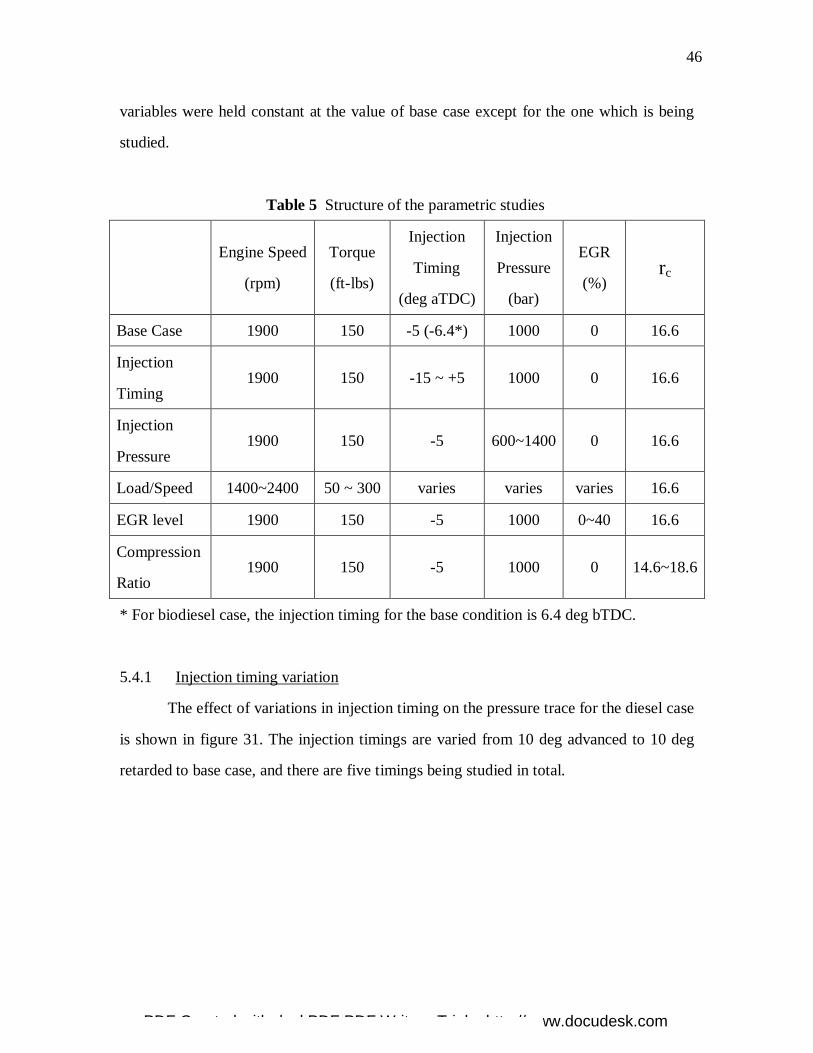
46
variables were held constant at the value of base case except for the one which is being
studied.
Table 5 Structure of the parametric studies
Engine Speed
(rpm)
Torque
(ft-lbs)
Injection
Timing
(deg aTDC)
Injection
Pressure
(bar)
EGR
(%) rc
Base Case 1900 150 -5 (-6.4*) 1000 0 16.6
Injection
Timing 1900 150 -15 ~ +5 1000 0 16.6
Injection
Pressure 1900 150 -5 600~1400 0 16.6
Load/Speed 1400~2400 50 ~ 300 varies varies varies 16.6
EGR level 1900 150 -5 1000 0~40 16.6
Compression
Ratio 1900 150 -5 1000 0 14.6~18.6
* For biodiesel case, the injection timing for the base condition is 6.4 deg bTDC.
5.4.1 Injection timing variation
The effect of variations in injection timing on the pressure trace for the diesel case
is shown in figure 31. The injection timings are varied from 10 deg advanced to 10 deg
retarded to base case, and there are five timings being studied in total.
PDF Created with deskPDF PDF Writer - Trial :: http://www.docudesk.com
Junnian
Rectangle

47
Fig.31 Pressure diagram for different injection timing, diesel case
Advanced injection timing leads to higher in-cylinder pressure while retarded
injection timing lowers the pressure. This effect can be attributed to the start of
combustion in the cylinder. If fuel is injected into the cylinder early, the combustion starts
during the compression stroke, and thereafter gas pressure and temperature increase
rapidly due to combustion. In the mean time, the piston continues going up which cause
the gas pressure and temperature to increase more rapidly. These two effects combine
together and then create a high peak in gas pressure. On the other hand, if the combustion
start is after TDC (top dead center), the pressure decreases due to expansion offset the
pressure rises due to combustion, which leads to a relatively lower gas pressure. If the
injection is retarded too much, as can be seen in the “10 deg retarded” case, the pressure
trace in-cylinder would show two peaks rather than one peak as for the other cases. The
first peak is mostly due to the compression stroke and the second peak is due to the heat
release (combustion).
0
20
40
60
80
100
120
-180 -120 -60 0 60 120 180
Pre
ssu
re (
ba
r)
Crank Angle (deg)
Results for diesel case 10 deg advanced
5 deg advanced
Base Case
5 deg retarded
10 deg retarded
PDF Created with deskPDF PDF Writer - Trial :: http://www.docudesk.com
Junnian
Rectangle

48
Fig.32 Pressure diagram for different injection timing, biodiesel case
For biodiesel case, figure 32 shows the effect of injection timing variation on the
pressure diagram. The effect of injection timing for the biodiesel case is very similar to
that of diesel case, except that the absolute values may not be the same. The 10 deg
advanced injection timing approximately increases the peak of gas pressure by 30%,
while the 10 deg retarded injection timing lowers the peak pressure by about 20% (and
creates an additional peak). As documented earlier, the timing of combustion start is the
major factor affecting the pressure diagram.
The effect of injection timing on ignition delay is showed in figure 33 and results
for diesel and biodiesel case are compared. From the plot, ignition delay increases when
retarding the injection timing from the base timing, and ignition delay also increases
when advancing the injection timing from the base case. This is a very typical plot in
engine operation and there is a “best” timing (at which the engine has the shortest
ignition delay). Too advanced injection timing leads to longer mixing time due to low
temperature and low pressure in the cylinder, and therefore leads to longer ignition delay.
0
20
40
60
80
100
120
-180 -120 -60 0 60 120 180
Pre
ssu
re (
ba
r)
Crank Angle (deg)
Results for biodiesel case 10 deg advanced
5 deg advanced
Base Case
5 deg retarded
10 deg retarded
PDF Created with deskPDF PDF Writer - Trial :: http://www.docudesk.com
Junnian
Rectangle

49
For the similar reason, when injection timing is retarded to very late, ignition delay will
also increase due to decreasing pressure and temperature in the cylinder. Comparing the
biodiesel results with the diesel results, shows that the trends of ignition delay change are
pretty similar to each other, while the biodiesel fueled cases have relatively longer
ignition delay than those of diesel fueled cases.
Fig.33 Ignition delay for different injection timings
Fig.34 Brake specific fuel consumption for different injection
timings
Figure 34 shows the brake specific fuel consumption (bsfc) as a function of
injection timing. bsfc indicates the fuel economy of an engine at specific operating
condition. Usually bsfc is minimized at MBT (maximum brake torque) timing, and if
injection timing is retarded or advanced to MBT timing the bsfc increase. The trend can
be clearly found in the plot above.
Figure 35 shows the ISNO2 (indicated specific nitrogen dioxide) with respect to
injection timings for both biodiesel fueled and diesel fueled cases. In direct injection
compression ignition engines, nitric oxides formation largely depends on how high the
gas temperature (combustion temperature) is and how long the temperature maintains. As
4
4.5
5
5.5
6
6.5
7
7.5
10 adv 5 adv Base 5 retard 10 retard
Igni
tion
Del
ay
Ref Diesel
Biodiesel
200
220
240
260
280
300
320
340
360
10 adv 5 adv Base 5 retard 10 retard
BS
fc (g
/kW
-h)
Ref Diesel
Biodiesel
PDF Created with deskPDF PDF Writer - Trial :: http://www.docudesk.com
Junnian
Rectangle
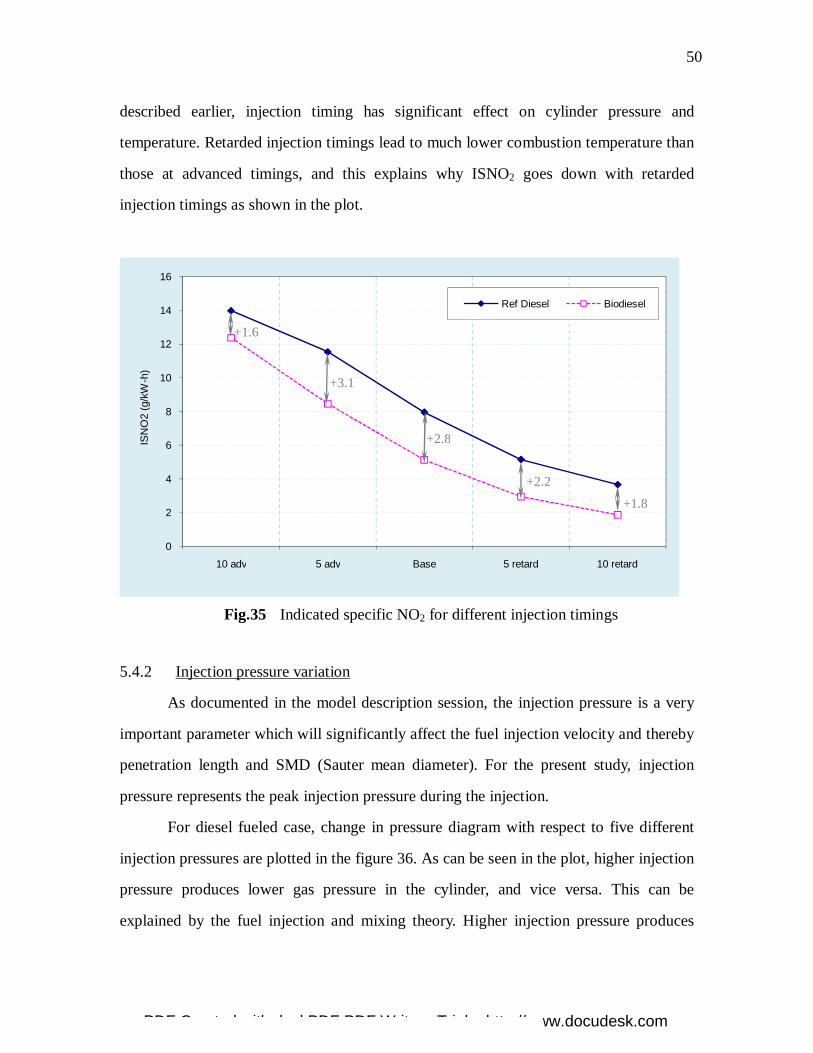
50
described earlier, injection timing has significant effect on cylinder pressure and
temperature. Retarded injection timings lead to much lower combustion temperature than
those at advanced timings, and this explains why ISNO2 goes down with retarded
injection timings as shown in the plot.
Fig.35 Indicated specific NO2 for different injection timings
5.4.2 Injection pressure variation
As documented in the model description session, the injection pressure is a very
important parameter which will significantly affect the fuel injection velocity and thereby
penetration length and SMD (Sauter mean diameter). For the present study, injection
pressure represents the peak injection pressure during the injection.
For diesel fueled case, change in pressure diagram with respect to five different
injection pressures are plotted in the figure 36. As can be seen in the plot, higher injection
pressure produces lower gas pressure in the cylinder, and vice versa. This can be
explained by the fuel injection and mixing theory. Higher injection pressure produces
0
2
4
6
8
10
12
14
16
10 adv 5 adv Base 5 retard 10 retard
ISN
O2
(g/k
W-h
)
Ref Diesel Biodiesel
+1.6
+3.1
+2.8
+2.2
+1.8
PDF Created with deskPDF PDF Writer - Trial :: http://www.docudesk.com
Junnian
Rectangle

51
higher injection velocity, small SMD, and longer penetration length. These factors make
the mixing process quicker which means the combustible air/fuel mixture is prepared
more quickly, and finally ignition delay becomes shorter. In addition, shorter ignition
delay will lower the gas temperature and pressure.
Fig.36 Pressure diagram for different injection pressure, diesel case
Fig.37 Pressure diagram for different injection pressure, biodiesel case
0
20
40
60
80
100
120
-180 -120 -60 0 60 120 180
Pre
ssu
re (
ba
r)
Crank Angle (deg)
Results for diesel case 600 bar
800 bar
Base Case
1200 bar
1400 bar
0
10
20
30
40
50
60
70
80
90
100
-180 -120 -60 0 60 120 180
Pre
ssu
re (
ba
r)
Crank Angle (deg)
Results for biodiesel case 600 bar
800 bar
Base Case
1200 bar
1400 bar
PDF Created with deskPDF PDF Writer - Trial :: http://www.docudesk.com
Junnian
Rectangle

52
Very similar trends can be found for biodiesel fueled case as shown in figure 37.
Figures 38 and 39 show the change in ignition delay and bsfc with respect to injection
pressure, and trend has been discussed in the previous paragraph.
Fig.38 Ignition delay for different injection pressure
Fig.39 bsfc for different injection pressure
4
4.5
5
5.5
6
6.5
600 bar 800 bar Base 1200 bar 1400 bar
Igni
tion
Del
ay (
deg)
Ref Diesel
Biodiesel
200
220
240
260
280
300
320
340
360
600 bar 800 bar Base 1200 bar 1400 bar
BS
fc (g
/kW
-h)
Ref Diesel
Biodiesel
PDF Created with deskPDF PDF Writer - Trial :: http://www.docudesk.com
Junnian
Rectangle

53
Figure 40 shows the ISNO2 with respect to injection pressure. As documented
before, higher injection pressure makes the combustion temperature lower, and
combustion temperature is a key factor in nitric oxides formation. So, the ISNO2 value
decreases with the increase of injection pressure as seen in the plot. The trend is similar
for both biodiesel case and reference diesel cases; and the diesel cases always produce
higher ISNO2 than the biodiesel case. More discussion on this topic is included in the
next section regarding the emission formation.
Fig.40 Indicated specific NO2 for different injection pressure
5.4.3 Load/speed variation
The effect of engine speed on ignition delay at three different load conditions of
50 ft-lbs, 150 ft-lbs, and 300 ft-lbs for both diesel and biodiesel fueled case are plotted in
figure 41. The ignition delay increases with the corresponding increase in speed as well
as increase in load. In terms of absolute time of ignition delay rather than degree crank
0
2
4
6
8
10
12
600 bar 800 bar Base 1200 bar 1400 bar
ISN
O2
(g/k
W-h
)
Ref Diesel Biodiesel
+3.4
+3.0
+2.8 +2.7
+2.3
PDF Created with deskPDF PDF Writer - Trial :: http://www.docudesk.com
Junnian
Rectangle
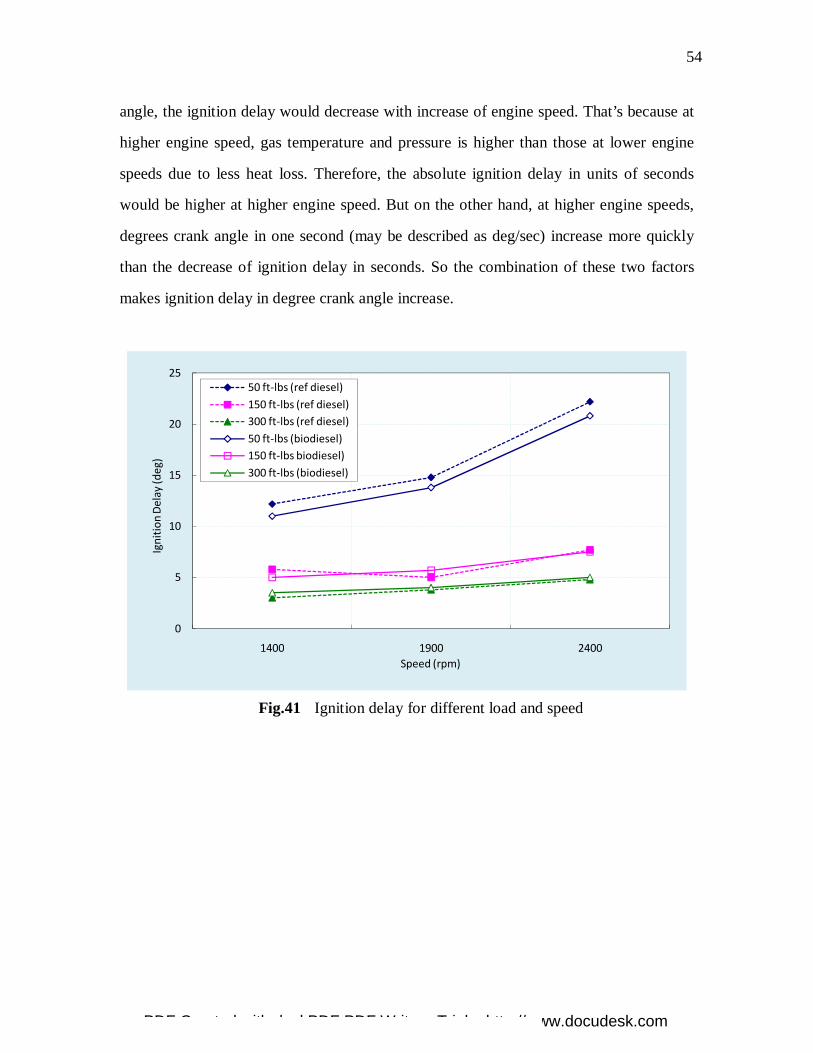
54
angle, the ignition delay would decrease with increase of engine speed. That’s because at
higher engine speed, gas temperature and pressure is higher than those at lower engine
speeds due to less heat loss. Therefore, the absolute ignition delay in units of seconds
would be higher at higher engine speed. But on the other hand, at higher engine speeds,
degrees crank angle in one second (may be described as deg/sec) increase more quickly
than the decrease of ignition delay in seconds. So the combination of these two factors
makes ignition delay in degree crank angle increase.
Fig.41 Ignition delay for different load and speed
0
5
10
15
20
25
1400 1900 2400
Ign
itio
n D
ela
y (
de
g)
Speed (rpm)
50 ft-lbs (ref diesel)
150 ft-lbs (ref diesel)
300 ft-lbs (ref diesel)
50 ft-lbs (biodiesel)
150 ft-lbs biodiesel)
300 ft-lbs (biodiesel)
PDF Created with deskPDF PDF Writer - Trial :: http://www.docudesk.com
Junnian
Rectangle
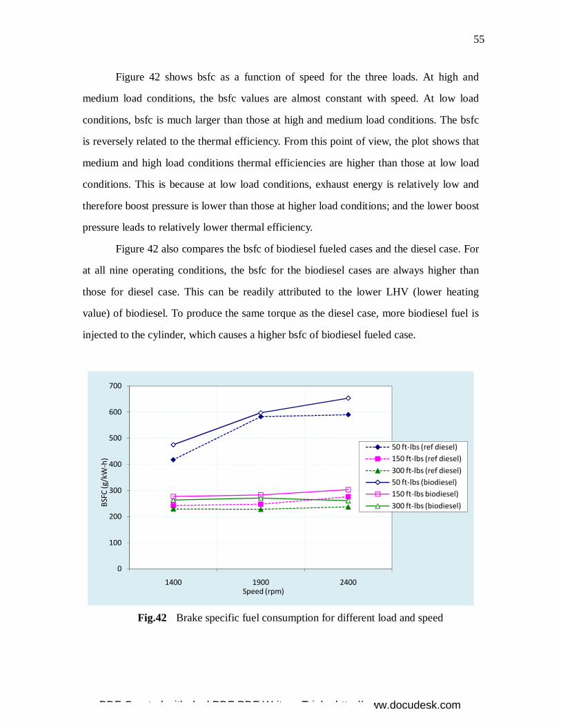
55
Figure 42 shows bsfc as a function of speed for the three loads. At high and
medium load conditions, the bsfc values are almost constant with speed. At low load
conditions, bsfc is much larger than those at high and medium load conditions. The bsfc
is reversely related to the thermal efficiency. From this point of view, the plot shows that
medium and high load conditions thermal efficiencies are higher than those at low load
conditions. This is because at low load conditions, exhaust energy is relatively low and
therefore boost pressure is lower than those at higher load conditions; and the lower boost
pressure leads to relatively lower thermal efficiency.
Figure 42 also compares the bsfc of biodiesel fueled cases and the diesel case. For
at all nine operating conditions, the bsfc for the biodiesel cases are always higher than
those for diesel case. This can be readily attributed to the lower LHV (lower heating
value) of biodiesel. To produce the same torque as the diesel case, more biodiesel fuel is
injected to the cylinder, which causes a higher bsfc of biodiesel fueled case.
Fig.42 Brake specific fuel consumption for different load and speed
0
100
200
300
400
500
600
700
1400 1900 2400
BSF
C (
g/k
W-h
)
Speed (rpm)
50 ft-lbs (ref diesel)
150 ft-lbs (ref diesel)
300 ft-lbs (ref diesel)
50 ft-lbs (biodiesel)
150 ft-lbs biodiesel)
300 ft-lbs (biodiesel)
PDF Created with deskPDF PDF Writer - Trial :: http://www.docudesk.com
Junnian
Rectangle

56
The EGR level applied at each operating conditions for diesel and biodiesel case
are shown in figures 43 and 44. For both the diesel and biodiesel cases, no EGR is
applied at low and medium load conditions, while 15%~25% EGR is used at high load
conditions. According to the plots, large amount of EGR are used at 6 high load
conditions (3 for diesel case and other 3 for biodiesel case), while at other conditions
almost no EGR is applied.
Fig.43 EGR level applied at each operating condition for reference diesel
case
Fig.44 EGR level applied at each operating condition for biodiesel case
0.00
5.00
10.00
15.00
20.00
25.00
30.00
50 150 300
EG
R (
%)
Torque (lb-ft)
1400 rpm
1900 rpm
2400 rpm
0.00
5.00
10.00
15.00
20.00
25.00
30.00
50 150 300
EG
R P
erce
ntag
e
Torque (ft-lbs)
1400
1900
2400
PDF Created with deskPDF PDF Writer - Trial :: http://www.docudesk.com
Junnian
Rectangle

57
Figure 45 shows ISNO2 as functions of engine speed for the three loads for diesel
and biodiesel fuels. The ISNO2 at medium load conditions are higher than those at low
and high load conditions. In general, all cases using diesel fuel produced higher NOx than
the biodiesel cases. Since the prediction of nitric oxides formation, even the measurement
of NOx at current stage of this study are still very preliminary, the simulation results has
a different trend with studies in most literatures, in which higher NOx emission for
biodiesel case is found.
Since EGR are only applied at high load conditions, ISNO2 values at 6 high load
conditions (three for diesel cases and three for biodiesel cases) are typically lower than
other cases due to EGR effect
Fig.45 Indicated specific NO2 for different load and speeds
0
1
2
3
4
5
6
7
8
9
1400 1900 2400
ISN
O2
(g
/kW
-h)
Speed (rpm)
50 ft-lbs (ref diesel)
150 ft-lbs (ref diesel)
300 ft-lbs (ref diesel)
50 ft-lbs (biodiesel)
150 ft-lbs biodiesel)
300 ft-lbs (biodiesel)
PDF Created with deskPDF PDF Writer - Trial :: http://www.docudesk.com
Junnian
Rectangle
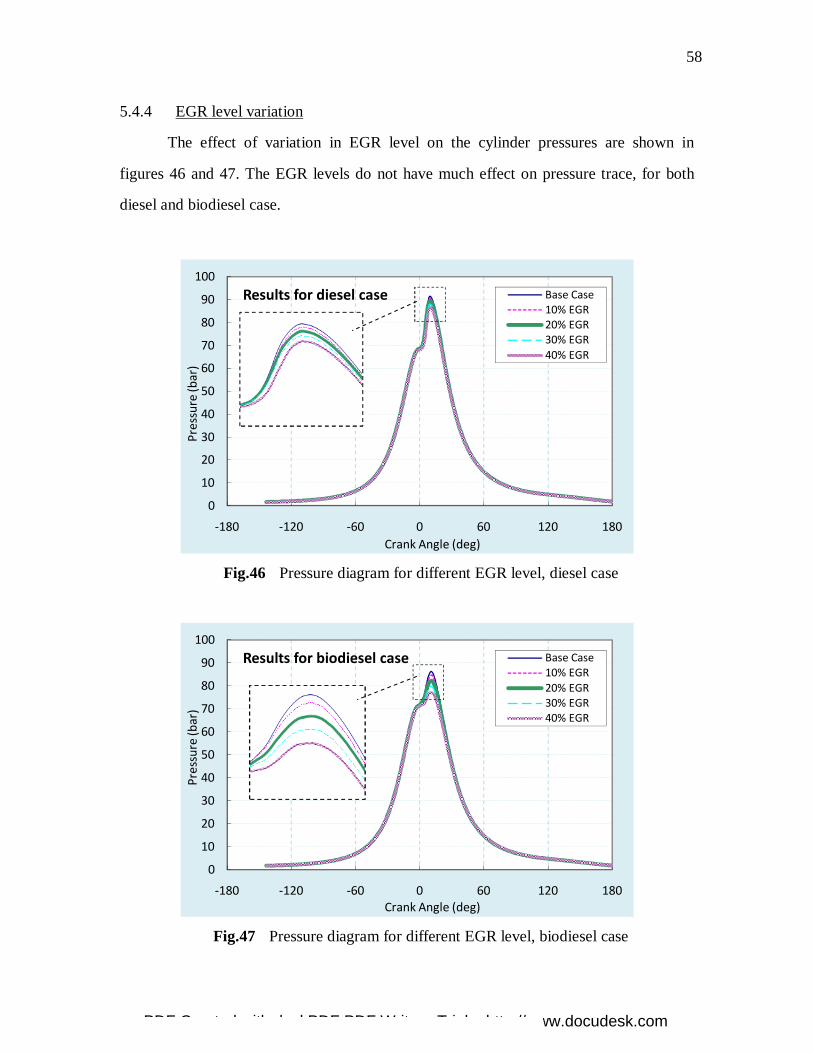
58
5.4.4 EGR level variation
The effect of variation in EGR level on the cylinder pressures are shown in
figures 46 and 47. The EGR levels do not have much effect on pressure trace, for both
diesel and biodiesel case.
Fig.46 Pressure diagram for different EGR level, diesel case
Fig.47 Pressure diagram for different EGR level, biodiesel case
0
10
20
30
40
50
60
70
80
90
100
-180 -120 -60 0 60 120 180
Pre
ssu
re (
ba
r)
Crank Angle (deg)
Results for diesel case Base Case
10% EGR
20% EGR
30% EGR
40% EGR
0
10
20
30
40
50
60
70
80
90
100
-180 -120 -60 0 60 120 180
Pre
ssu
re (
ba
r)
Crank Angle (deg)
Results for biodiesel case Base Case
10% EGR
20% EGR
30% EGR
40% EGR
PDF Created with deskPDF PDF Writer - Trial :: http://www.docudesk.com
Junnian
Rectangle

59
Fig.48 Ignition delay for different EGR level
Fig.49 Brake specific fuel consumption for different EGR level
Fig.50 Indicated specific NO2 for different EGR level
Figures 48 and 49 show the effect of EGR level on ignition delay and bsfc.
Similar to the previous two plots, no significant effect caused by EGR level are noted.
Hot EGR gases causes some difference in ignition delay but the effect is small. Similarly,
4
4.4
4.8
5.2
5.6
6
0 5 10 15 20 25
Ign
itio
n D
ela
y (
de
g)
EGR Percentage
Ref Diesel
Biodiesel
200
220
240
260
280
300
320
340
360
0 5 10 15 20 25
BSf
c (g
/kW
-h)
EGR Percentage
Ref Diesel
Biodiesel
0
1
2
3
4
5
6
7
8
9
0 5 10 15 20 25
ISN
O2
(g
/kW
-h)
EGR Percentage
Ref Diesel Biodiesel
+2.8
+3.1
+2.7
+1.9 +1.2
PDF Created with deskPDF PDF Writer - Trial :: http://www.docudesk.com
Junnian
Rectangle

60
increasing EGR level leads to slightly increase of bsfc. Figure 50 shows effect of EGR
level on NOx. As known by all, EGR is designed to depress the formation of NOx. This
can be seen in the plot for diesel and biodiesel case.
5.4.5 Compression ratio variation
The parametric study for compression ratio variation is more conceptual than the
above ones, since for a real engine, compression ratio of the engine is fixed unless there
is a variable compression ratio feature.
Figures 51 and 52 show the effect of compression ratio on the cylinder pressures
for diesel and biodiesel cases. Clearly, the pressures increase with the increase of
compression ratio. This can be easily attributed to the ideal gas law which states pressure
is reversely proportional to volume. Very similar trend is found both in diesel and
biodiesel case.
Fig.51 Pressure diagram for different compression ratio, diesel case
0
20
40
60
80
100
120
-180 -120 -60 0 60 120 180
Pre
ssu
re (
ba
r)
Crank Angle (deg)
Results for diesel case rc=14.6
rc=15.6
Base Case
rc=17.6
rc=18.6
PDF Created with deskPDF PDF Writer - Trial :: http://www.docudesk.com
Junnian
Rectangle

61
Fig.52 Pressure diagram for different compression ratio, biodiesel case
As documented earlier, higher compression ratio produces higher pressure and
temperature by the end of compression. Then, the higher pressures and temperatures
make the mixing of fuel and air more rapid and more combustible, and finally leads to
low ignition delay. This is showed in figure 53.
Fig.53 Ignition delay for different compression ratio
Fig.54 bsfc for different compression ratio
0
20
40
60
80
100
120
-180 -120 -60 0 60 120 180
Pre
ssu
re (
ba
r)
Crank Angle (deg)
Results for biodiesel case rc=14.6
rc=15.6
Base Case
rc=17.6
rc=18.6
4
4.5
5
5.5
6
6.5
7
14 15 16 17 18 19
Ign
itio
n D
ela
y (
de
g)
Compression Ratio
Ref Diesel
Biodiesel
200
220
240
260
280
300
320
14 15 16 17 18 19
BSf
c (g
/kW
-h)
Compression Ratio
Ref Diesel
Biodiesel
PDF Created with deskPDF PDF Writer - Trial :: http://www.docudesk.com
Junnian
Rectangle

62
Figure 54 on the previous page shows the change in bsfc with respect to
compression ratio. The increase of compression ratio produces higher pressure as shown
previously which means higher power is generated with the same amount of fuel. Since
bsfc is defined as fuel consumption divided by brake power, the bsfc decreases with the
increase of compression ratio.
Effect of compression ratio on nitric oxides emission is also investigated, as
shown in figure 55 higher gas temperature due to higher compression ratio is the main
reason why ISNO2 increases with the rise of compression ratio.
Fig.55 Indicated specific NO2 for different compression ratio
4
5
6
7
8
9
10
14 15 16 17 18 19
ISN
O2
(g
/kW
-h)
Compression Ratio
Ref Diesel Biodiesel
+2.2 +2.5
+2.8
+3.2
+3.4
PDF Created with deskPDF PDF Writer - Trial :: http://www.docudesk.com
Junnian
Rectangle

63
5.5 Numerical study focusing on NOx emission
As documented earlier, biodiesel characteristically has lower particulate matter
(PM) emissions, suggesting that characteristics of NOx emission from biodiesel would be
very crucial for the use of biodiesel fueled direct injection compression ignition engines.
In present study, though one-dimensional engine model cannot accurate predict the NOx
emission, it would be very useful to study how individual mechanism or parameter affect
nitric oxides emission.
5.5.1 Sensitivity of NOx prediction on major parameters
Based on a reference condition (1900 rpm 150 ft-lb), effect of change in several
major parameters on NOx emission has been studied. The results are listed in the table 6
in the next page.
Among the six parameters that have been studied, radiation multiplier, wall
temperature, and compression ratio are more conceptual ones. Radiation multiplier
adjusts the amount of radiation heat transfer from high temperature gas in the cylinder to
the cylinder wall. Less radiation heat transfer increases the NOx emission by 10 to 15
percent. This result is of interest because it is believed by some investigators that
biodiesel combustion has less radiative heat transfer due to its lower PM emission.
Similar to the radiation multiplier, wall temperature and compression ratio are also not
very sensitive to NOx emission. These two parameters, to some extent, affect the gas
temperature in the cylinder and finally affect the nitric oxides formation. In the above
studied six parameters, both EGR level and injection timing has greatest effect on the
NOx produced. A little adjustment could result in over 50% change in specific nitric
oxides.
PDF Created with deskPDF PDF Writer - Trial :: http://www.docudesk.com
Junnian
Rectangle

64
Table 6 How adjustable parameters affect the NOx calculation
Items Change in ISNO2 (g/kW-h)
Diesel Biodiesel
Radiation Multiplier (from 1 to 0) + 13.8% + 15.6%
Radiation Multiplier (from 1 to 2) -12.2% - 14.3%
Start of Injection (5 deg advance) + 45.16% + 65.04%
Start of Injection (5 deg retard) - 35.22% - 42.58%
Injection Pressure (from 1000 bar to 800 bar) + 15.35% + 20.22%
Injection Pressure (from 1000 bar to 1200 bar) - 10.57% - 14.06%
Wall Temperature (from 450 K to 400 K) -11.1% - 12.0%
Wall Temperature (from 450 K to 500 K) + 12.1% + 12.9%
Compression Ratio (from 16.6 to 15.6) - 9.06% - 10.57%
Compression Ratio (from 16.6 to 17.6) + 8.20% + 8.79%
EGR Level (from 10% to 0%) + 41.21% + 100.00%
EGR Level (from 10% to 20%) - 34.28% - 58.98%
5.5.2 Numerical study of five NOx kinetics
As discussed earlier, in the present study the calculation of NOx is based on the
extended Zeldovich mechanism which includes three NO formation reactions. The rate
constant of each reaction, have been determined by many investigators [24, 26, 27, 28,
29]. Here five most widely-used kinetics (rate constants set) recommended by different
investigators are applied to calculate NOx in the GT-Power simulation. The following
table shows the details of each kinetics and its realization in GT-Power.
PDF Created with deskPDF PDF Writer - Trial :: http://www.docudesk.com
Junnian
Rectangle

65
Table 7 The NOx kinetics studied and their realization in GT-Power
Kinetics Realization in GT-Power
Number Reaction Rate Constant F A Approximation
Heywood
[24]
No.1 O+N2=NO+N 7.6*1013exp(-38000/T) 1 1
No.2 N+O2=NO+O 6.4*1009Texp(-3150/T) 1 1
No.3 N+OH=NO+H 4.1*1013 1 N/A
Baulch
[26]
No.1 O+N2=NO+N 7.6*1013exp(-38000/T) 1 1
No.2 N+O2=NO+O 6.4*1009Texp(-3150/T) 1 1
No.3 N+OH=NO+H N/A 0 N/A
H&S
[27]
No.1 O+N2=NO+N 1.82*1014exp(-38350/T) 2.39 1.01
No.2 N+O2=NO+O 1.80*1010Texp(-4680/T) 2.81 1.49
No.3 N+OH=NO+H 1.10*1014exp(-1260/T) 0.47 N/A Yes
M&B
[28]
No.1 O+N2=NO+N 1.55*1013T0.3exp(-37945/T) 2.3 1 Yes
No.2 N+O2=NO+O 6.4*1009Texp(-3160/T) 1 1
No.3 N+OH=NO+H 3.8*1013 0.93 N/A
D&B
[29]
No.1 O+N2=NO+N 1.95*1014exp(-38660/T) 2.57 1.02
No.2 N+O2=NO+O 9.0*1009exp(-3270/T) 1.41 1.04
No.3 N+OH=NO+H 1.10*1014exp(-565/T) 0.62 N/A Yes
Since the NO model in GT-Power offers only 5 adjustable rate constants in the
kinetics, while some of the kinetics needs six of them, some approximation for H&S,
M&B, and D&B kinetics are made, as shown in the figures 56 and 57. For the first rate
constant of M&B kinetics, an exponential function is used to approximate the product of
a polynomial and an exponential function (figure 56). For the third rate constants of H&S
and D&B kinetics, two constants are used to approximate the corresponding exponential
functions.
PDF Created with deskPDF PDF Writer - Trial :: http://www.docudesk.com
Junnian
Rectangle

66
Fig.56 The approximation of M&B kinetics in GT-Power
Fig.57 The approximations of H&B and D&B kinetics in GT-Power
Figure 58 shows the comparison between five nitric oxides kinetics for the
reference diesel case at the base case described earlier. It clearly shows that the shape of
NO concentration history in the cylinder are very similar to each other for different
kinetics. Among the five kinetics, “M&B” predicted the highest “frozen concentration” of
NO, while “Baulch” gave the lowest NO concentration.
Fig.58 Comparison of NO calculation with different NO kinetics, diesel case
1.E+05
1.E+06
1.E+07
1.E+08
1.E+09
2000 2200 2400 2600 2800 3000
Ra
te C
on
sta
nt
Temperature (K)
M&B_RateConst_1
GT_F1=2.3_A1=1.0
5E+13
6E+13
7E+13
8E+13
9E+13
1E+14
2000 2200 2400 2600 2800 3000
Ra
te C
on
sta
nt
Temperature (K)
H&S_RateConst
_No.3
D&B_RateCons
t_No.3
GT_F3=0.4688
GT_F3=0.6208
0
100
200
300
400
500
-180 -120 -60 0 60 120 180
NO
Co
nce
ntr
ati
on
(p
pm
)
Crank Angle (deg)
Results for diesel case
Heywood Kinetics
Baulch Kinetics
H&S Kinetics
M&B Kinetics
D&B Kinetics
PDF Created with deskPDF PDF Writer - Trial :: http://www.docudesk.com
Junnian
Rectangle

67
For the biodiesel case in figure 59, very similar results were obtained for the same
five NO kinetics. The study of nitric kinetics indicates that at same operating conditions,
different kinetics which means different rate constants could results in large difference in
NO calculation. The highest value calculated by M&B kinetics is almost twice as the
value calculated by Baulch kinetics.
Fig.59 Comparison of NO calculation with different NO kinetics, biodiesel case
0
100
200
300
400
500
-180 -120 -60 0 60 120 180
NO
co
nce
ntr
ati
on
(p
pm
)
Crank Angle (deg)
Results for biodiesel case
Heywood Kinetics
Baulch Kinetics
H&S Kinetics
M&B Kinetics
D&B Kinetics
PDF Created with deskPDF PDF Writer - Trial :: http://www.docudesk.com
Junnian
Rectangle

68
6. CONCLUSIONS AND RECOMMENDATIONS
A quasi-dimensional, multi-zone engine model of a four stroke
compression-ignition engine was developed and applied to study the engine performance
and emission characteristics with both reference diesel fuel and biodiesel fuel. At nine
typical operating conditions, the engine model was calibrated for both diesel and
biodiesel fuels. Pressure diagram and heat release curves at these operating conditions
were compared between simulation and experiments. In addition, variations in pressure
trace, ignition delay, brake specific fuel consumption, indicated specific nitrogen dioxide
with respect to injection timing, injection pressure, load and speed, compression ratio,
and percentage of exhaust gas recirculation were determined from both simulations with
diesel and biodiesel fuel. Furthermore, focusing nitric oxides, the sensitivity studies and
NO kinetics studies were made for both diesel and biodiesel case, and the results were
compared between each other. Major results and conclusions can be summarized as
follows:
1. The calibrated quasi-dimensional multi-zone model successfully predicted engine
performance for both diesel and biodiesel fueled engine. Simulated pressure diagram and
heat release curve at nine operating conditions showed good agreement with
experimentally determined results.
2. Injection timing and compression ratio has the most significant effect on pressure
diagram for both diesel and biodiesel fueled engine. Advanced injection timing and
higher compression ratio leads to higher in-cylinder pressure, while retarded injection
timing and small compression ratio lowers the pressure diagram. Comparing between
diesel and biodiesel case, pressure diagram with biodiesel has lower peak pressure than
that with reference diesel fuel for all the operating conditions and the parameters
PDF Created with deskPDF PDF Writer - Trial :: http://www.docudesk.com
Junnian
Rectangle

69
considered for investigation. This observation might be attributed to the lower calorific
value of biodiesel relative to diesel fuel.
3. The ignition delays for biodiesel fueled case were higher (3% ~ 10%) than the
corresponding values for the diesel fueled case for medium load and high load conditions.
In addition, variations in injection timing, injection pressure, and compression ratio
would have certain effects (0.5~1.5 degree crank angle) on ignition delay for both
biodiesel and diesel case.
4. The brake specific fuel consumption (bsfc) values for the biodiesel fueled engine were
consistently higher (2%~12%) than the corresponding values for the diesel fueled case
for all operating conditions and parameters studied. This results can be attributed to lower
LHV of biodiesel. To achieve the same power output, more biodiesel fuel is required.
5. Results from sensitivity study shows injection timing and EGR percentage has the
most significant effect on nitric oxides calculation (50%~100%) among the six
parameters that is studied. In addition, changes in most of the parameters has greater
effect on biodiesel fueled engine than the corresponding effect on diesel case. The NO
kinetics study indicates that at the same base case, M&B kinetics predicted highest NO
value while Baulch kinetics gave the lowest value.
PDF Created with deskPDF PDF Writer - Trial :: http://www.docudesk.com
Junnian
Rectangle
70
Due to the unknown characteristics of the biodiesel fuel, some observations from
both the simulation and the experiment still cannot be well explained. With more accurate
experimental data, recommendations for future work are,
1. Calibrate the model to match the emission data from experiment, especially the nitric
oxides emission. Together with burned zone temperature profile, compare the results with
diesel and biodiesel fueled engine and find out the cause of the difference if there is any.
2. After getting the map for rack position of the VGT, include the compressor and turbine
in the simulation rather than using compressor-out condition and turbine-in condition as
inputs.
3. To get better understanding of biodiesel combustion in the cylinder, it would be useful
to integrate the 3D computational fluid mechanics and detailed chemical kinetics into the
current one-dimensional engine model. The simulation of intake/exhaust system could
still be one-dimensional and the combustion in the cylinder could be simulated by 3D
CFD and detailed chemical kinetics.
PDF Created with deskPDF PDF Writer - Trial :: http://www.docudesk.com
Junnian
Rectangle

71
REFERENCES
1 US Department of Energy, Energy Information Administration, Available: http://www.eia.doe.gov/emeu/aer/pdf/pages/sec1.pdf, Accessed: 01/08/2009.
2 Smaling, R. Biodiesel and air quality: HARC Brownbag Presentation, Available: files.harc.edu/Documents/Announcements/2006/BiodieselAndAirQuality.pdf, Accessed: 03/22/2009.
3 Monyem, A., Van Gerpen, J. H., and Canakci, M. The effect of timing and oxidation on emissions from biodiesel--fueled engines. Trans. of the ASAE, 2001, 44 (1), 35–42.
4 Tat, M. E., Van Gerpen, J. H., and Wang, P. S. Fuel property effects on injection timing, ignition timing, and oxides of nitrogen emissions from biodiesel--fueled engines. Transactions of the ASAE, 2007, 50 (4), 1123-1128.
5 Lu, X. M., Ge, Y. S., Wu, S. J., and Han, X. K. An experimental investigation on combustion and emissions characteristics of turbocharged DI engines fueled with blends of biodiesel. SAE paper 2005-01-2199, 2005.
6 Yuan, W. Q., Hansen, C. A., and Zhang, Q. Computational modeling of NOx emissions from biodiesel combustion. International Journal of Vehicle Design, 2007, 45 (1/2), 12-32.
7 Szybist, P. J., Kirby, R. S., and Boehman, L. A. NOx emissions of alternative diesel fuels: a comparative analysis of biodiesel and FT diesel. Energy & Fuels, 2005, 19, 1484-1492.
8 Wayne, A. E. Effects of methyl ester biodiesel blends on NOx emissions. SAE paper 2008-01-0078, 2008.
9 Chang, Y. Z., and Van Gerpen, J. H. Fuel properties and engine performance for biodiesel prepared from modified feedstock. SAE paper 971684, 1997.
10 Senatore, A., Cardone, M., Rocco, V., and Prati, V. M. A comparative analysis of combustion process in DI diesel engine fueled with biodiesel and diesel fuel. SAE paper 2000-01-0691, 2000.
PDF Created with deskPDF PDF Writer - Trial :: http://www.docudesk.com
Junnian
Rectangle

72
11 Parvate-Patil, G., Vasquez, M., and Payne, M. Effects of Different Biodiesel Blends on Heat Release and its Related Parameters. ASME Internal Combustion Engine Division 2006 Fall Technical Conference, November 5-8, 2006, Sacramento, California, USA.
12 Kinoshita, E., Myo, T., Hamasaki, K., Tajima, H., and Zhang, R. K. Diesel combustion characteristics of coconut oil and palm oil biodiesels. SAE paper 2006-01-3251, 2006.
13 Ban-Weiss, G. A., Chen, J. Y., Buchholz, B. A., and Dibble, R. W. A numerical investigation into the anomalous slight NOx increase when burning biodiesel, a new theory. Fuel Processing Technology, 2007, 88(7), 659-667.
14 Agarwal, A. Biofuels (alcohols and biodiesel) applications as fuels for internal combustion engines. Progress in Energy and Combustion Science, 2007, 33, 233–271.
15 Musculus, M. Measurements of the influence of soot radiation on in-cylinder temperatures and exhaust NOx in a heavy-duty DI diesel engine. SAE paper 2005-01-0925, 2005.
16 Yamane, K. Influence of physical and chemical properties of biodiesel fuels on injection, combustin and exhaust emission characteristics in a direct injection compression ignition engine. International Journal of Engine Research, 2001, 2(4), 249-261
17 Jung, D., and Assanis, D. Multi-zone DI diesel spray combustion model for cycle simulation studies of engine performance and emissions. SAE paper 2001-01-1246, 2001.
18 Arsie, I., Di Genova, F., Mogavero, A., Pianese, C., and Rizzo, G. Multi-zone predictive modeling of common rail multi-injection diesel engine. SAE paper 2006-01-1384, 2006.
19 Kouremenos, D., Rakopoulos, C., and Hountalas, D. Multi-zone combustion modeling for the prediction of pollutants emissions and performance of DI diesel engines. SAE paper 970635, 1997.
20 McCrady, J., Hansen, A., and Lee, C. Modeling biodiesel combustion using GT-Power. ASABE Meeting Presentation, Paper Number 076095.
PDF Created with deskPDF PDF Writer - Trial :: http://www.docudesk.com
Junnian
Rectangle

73
21 GT-Power User Manual, Version 6.2, Gamma Technology, Inc, September 2006.
22 Woschni, G. A universally applicable equation for the instantaneous heat transfer coefficient in the internal combustion engine. SAE Trans., 1967, 76, 3065.
23 Hohenberg, G. Advanced approaches for heat transfer calculations. SAE paper 790825, 1979.
24 Heywood, J. Internal Combustion Engine Fundamentals, 1988 (McGraw-Hill, New York).
25 Yoshizaki, T., Nishida, K., and Hiroyasu, H. Approach to low NOx and smoke emission engines by using phenomenological simulation. SAE Paper 930612, 1993.
26 Baluch, D. L., Drysdale, D. D., Horne, D. G., and Lloyd, A. C. Evaluated Kinetic Data for High Temperature Reactions, Vol. 2 – Homogeneous Gas Phase Reactions of the H2-N2-O2 System, 1973 (Butterworths & Co. Ltd, London).
27 Hanson, R. K. and Salimian, S. Survey of Rate Constants in the N/H/O System, in Combustion Chemistry, ed. W. C. Gardiner, Jr., 1984 (Springer-Verlag, New York).
28 Miller, J. A. and Bowman, C. T. Mechanism and modeling of nitrogen chemistry in combustion. Progress in Energy and Combustion Science, 1989, 15, 287-338.
29 Dean, A. M. and Bozzelli, J. W. Combustion Chemistry of Nitrogen, in Gas-Phase Combustion Chemistry, ed. W. C. Gardiner, Jr., 2000 (Springer-Verlag, New York).
PDF Created with deskPDF PDF Writer - Trial :: http://www.docudesk.com
Junnian
Rectangle

74
APPENDIX I
PROPERTIES OF BIODIESEL AND DIESEL FUEL
Table 8 Properties comparison between diesel 2 and biodiesel
State Item Unit Diesel No.2 Biodiesel
Vapor
C Atoms per Molecule 13.5 18.82
H Atoms per Molecule 23.6 34.39
O Atoms per Molecule 0 2
N Atoms per Molecule 0 0
Lower Heating Value kJ/kg 43250 37150
Critical Temperature K 569.4 785.87
Critical Pressure bar 24.6 12.07
Enthalpy kJ/kg See Table 9 See Table 9
Viscosity Pa-s See Table 10 See Table 11
Thermal Conductivity W/m-K See Table 10 See Table 11
Liquid
Heat of Vaporization kJ/kg 250 357
Density kg/m^3 830 890.7
Enthalpy kJ/kg See Table 12 See Table 12
Viscosity kg/m-s See Table 13 See Table 14
Thermal Conductivity W/m-K See Table 13 See Table 14
PDF Created with deskPDF PDF Writer - Trial :: http://www.docudesk.com
Junnian
Rectangle

75
Table 9 Enthalpy constants for vapor diesel and biodiesel
Enthalpy Constants Diesel No.2 Biodiesel
a1 1634.3 1675
a2 1.8191 1
a3 0 0
a4 0 0
a5 0 0
Note: The enthalpy of the vapor in J/kg is determined from the following curve-fit equation where href is the enthalpy at the reference temperature, Tref, of 298 K.
2 3 4 51 2 3 4 5( ) ( ) ( ) ( ) ( )ref ref ref ref ref refh h a T T a T T a T T a T T a T T− = − + − + − + − + −
Table 10 Viscosities and thermal conductivities of diesel vapor
Temperature Dynamic Viscosity Thermal Conductivity
[K] [Pa-s] [W/m-K]
303.15 8.02e-006 0.00829904
373.55 6.75e-006 0.00829904
475.35 475.35 475.35
Table 11 Viscosities and thermal conductivities of biodiesel vapor
Temperature Dynamic Viscosity Thermal Conductivity
[K] [Pa-s] [W/m-K]
617 8.05715E-05 0.023996841
620 8.09543E-05 0.024174589
640 8.34962E-05 0.025364339
660 8.60214E-05 0.026562371
PDF Created with deskPDF PDF Writer - Trial :: http://www.docudesk.com
Junnian
Rectangle

76
Table 11 Continued
680 8.85297E-05 0.027768685
700 9.10212E-05 0.02898328
720 9.34959E-05 0.030206157
740 9.59537E-05 0.031437315
760 9.83948E-05 0.032676755
780 0.000100819 0.033924477
800 0.000103226 0.03518048
820 0.000105617 0.036444765
840 0.000107991 0.037717331
860 0.000110348 0.038998179
880 0.000112688 0.040287309
900 0.000115011 0.04158472
920 0.000117318 0.042890413
940 0.000119608 0.044204387
960 0.000121881 0.045526643
980 0.000124137 0.046857181
1000 0.000126376 0.048196
Table 12 Enthalpy constants for liquid diesel and biodiesel
Enthalpy Constants Diesel No.2 Biodiesel
a1 2050 2050
a2 0 0
a3 0 0
Note: The enthalpy of the liquid in J/kg at pressure=1 bar is determined from the following curve-fit equation, where the reference enthalpy is defined as: href = (href)vapor - hvaporization and Tref = 298 K
2 31 2 3( ) ( ) ( )ref ref ref refh h a T T a T T a T T− = − + − + −
PDF Created with deskPDF PDF Writer - Trial :: http://www.docudesk.com
Junnian
Rectangle

77
Table 13 Viscosities and thermal conductivities of liquid diesel
Temperature Dynamic Viscosity Thermal Conductivity
[K] [Pa-s] [W/m-K]
273.15 0.00219 0.116645
290.15 0.00171 0.113925
310.15 0.00133 0.110725
330.15 0.0011 0.107525
350.15 0.00096 0.104325
373.15 0.00088 0.100645
400.15 0.00087 0.096325
450.15 0.00112 0.088325
Table 14 Viscosities and thermal conductivities of liquid biodiesel
Temperature Dynamic Viscosity Thermal Conductivity
[K] [Pa-s] [W/m-K]
300 0.000045993 0.17887
310 0.000036646 0.17719
320 0.00002994 0.17549
330 0.000024982 0.17377
340 0.000021223 0.17205
350 0.000018309 0.17031
360 0.000016007 0.16855
370 0.000014157 0.16678
380 0.000012649 0.165
390 0.000011402 0.1632
400 0.00001036 0.16139
410 0.00000948 0.15955
PDF Created with deskPDF PDF Writer - Trial :: http://www.docudesk.com
Junnian
Rectangle

78
Table 14 Continued
420 0.000008729 0.1577
430 0.000008083 0.15584
440 0.000007523 0.15395
450 0.000007034 0.15204
460 0.000006604 0.15011
470 0.000006224 0.14816
480 0.000005886 0.14618
490 0.000005584 0.14418
500 0.000005313 0.14216
510 0.000005069 0.14011
520 0.000004848 0.13803
530 0.000004647 0.13591
540 0.000004463 0.13377
550 0.000004296 0.13159
560 0.000004142 0.12937
570 0.000004 0.12711
580 0.000003869 0.12481
590 0.000003748 0.12247
600 0.000003636 0.12007
610 0.000003531 0.11762
620 0.000003434 0.11511
630 0.000003343 0.11253
640 0.000003259 0.10988
PDF Created with deskPDF PDF Writer - Trial :: http://www.docudesk.com
Junnian
Rectangle

79
APPENDIX II
DISCHARGE COEFFICIENTS WITH LIFT
Table 15 Intake valve flow coefficients
L/D Ratio Forward Flow Coefficient Reverse Flow Coefficient
0 0 0
0.0304053 0.1071826 0.1071826
0.0608812 0.2031018 0.2031018
0.0911371 0.2788924 0.2788924
0.1215096 0.3513742 0.3513742
0.1519005 0.4214792 0.4214792
0.1823885 0.4814215 0.4814215
0.2128395 0.5291767 0.5291767
0.243119 0.5648113 0.5648113
0.2734641 0.5883421 0.5883421
0.3038992 0.6019374 0.6019374
0.3344928 0.6113458 0.6113458
0.3646257 0.6184707 0.6184707
0.3952485 0.6262355 0.6262355
Table 16 Exhaust valve flow coefficients
L/D Ratio Forward Flow Coefficient Reverse Flow Coefficient
0 0 0
0.0309989 0.1052954 0.1052954
0.0620698 0.2117053 0.2117053
PDF Created with deskPDF PDF Writer - Trial :: http://www.docudesk.com
Junnian
Rectangle

80
Table 16 Continued
0.0929163 0.3008259 0.3008259
0.1238818 0.385439 0.385439
0.154866 0.4794244 0.4794244
0.1859492 0.5483239 0.5483239
0.2169947 0.5985104 0.5985104
0.2478653 0.6431867 0.6431867
0.2788029 0.6792136 0.6792136
0.3098321 0.7080437 0.7080437
0.341023 0.733009 0.733009
0.3717443 0.7526495 0.7526495
0.4029648 0.7682453 0.7682453
Fig.60 Discharge coefficients against L/D ratio for intake and exhaust valves
0
0.1
0.2
0.3
0.4
0.5
0.6
0.7
0.8
0.9
0 0.05 0.1 0.15 0.2 0.25 0.3 0.35 0.4 0.45
Dis
cha
rge
Co
eff
icie
nt
L/D Ratio
Exhaust Valve
Intake Valve
PDF Created with deskPDF PDF Writer - Trial :: http://www.docudesk.com
Junnian
Rectangle

81
APPENDIX III
MODEL VALIDATION FOR BIODIESEL FUEL
Fig.61 Pressure diagram comparison @ 1400 rpm 50 ft-lbs for biodiesel
Fig.62 Heat release curve comparison @ 1400 rpm 50 ft-lbs for biodiesel
Fig.63 Pressure diagram comparison @ 1400 rpm 150 ft-lbs for biodiesel case
Fig.64 Heat release curve comparison @ 1400 rpm 150 ft-lbs for biodiesel
case
0
10
20
30
40
50
60
70
-180 -120 -60 0 60 120 180
Pre
ssu
re (
ba
r)
Crank Angle (deg)
Pressure Diagram @ 1400 rpm 50 ft-lb
(bio)
Exp
Sim
-0.01
0
0.01
0.02
0.03
0.04
0.05
0.06
0.07
0.08
-180 -120 -60 0 60 120 180R
OH
R (
1/d
eg
)Crank Angle (deg)
Heat Release Comparison @1400 rpm
50 ft-lb (bio)
"Experiment"
Simulation
0
10
20
30
40
50
60
70
80
90
-180 -120 -60 0 60 120 180
Pre
ssu
re (
ba
r)
Crank Angle (deg)
Pressure Diagram @ 1400 rpm 150 ft-
lb (bio)
Exp
Sim
-0.02
0
0.02
0.04
0.06
0.08
0.1
-180 -120 -60 0 60 120 180
RO
HR
(1
/de
g)
Crank Angle (deg)
Heat Release Comparison @1400 rpm
150 ft-lb (bio)
"Experiment"
Simulation
PDF Created with deskPDF PDF Writer - Trial :: http://www.docudesk.com
Junnian
Rectangle

82
Fig.65 Pressure diagram comparison @ 1400 rpm 300 ft-lbs for biodiesel case
Fig.66 Heat release curve comparison @ 1400 rpm 300 ft-lbs for biodiesel
case
Fig.67 Pressure diagram comparison @ 1900 rpm 50 ft-lbs for biodiesel case
Fig.68 Heat release curve comparison @ 1900 rpm 50 ft-lbs for biodiesel case
0
20
40
60
80
100
-180 -120 -60 0 60 120 180
Pre
ssu
re (
ba
r)
Crank Angle (deg)
Pressure Diagram @ 1400 rpm 300 ft-
lb (bio)
Exp
Sim
-0.01
0
0.01
0.02
0.03
0.04
0.05
0.06
-180 -120 -60 0 60 120 180
RO
HR
(1
/de
g)
Crank Angle (deg)
Heat Release Comparison @1400 rpm
300 ft-lb (bio)
"Experiment"
Simulation
0
10
20
30
40
50
60
70
80
-180 -120 -60 0 60 120 180
Pre
ssu
re (
ba
r)
Crank Angle (deg)
Pressure Diagram @ 1900 rpm 50 ft-lb
(bio)
Exp
Sim
-0.01
0
0.01
0.02
0.03
0.04
0.05
0.06
0.07
0.08
0.09
-180 -120 -60 0 60 120 180
RO
HR
(1
/de
g)
Crank Angle (deg)
Heat Release Comparison @1900 rpm
50 ft-lb (bio)
"Experiment"
Simulation
PDF Created with deskPDF PDF Writer - Trial :: http://www.docudesk.com
Junnian
Rectangle

83
Fig.69 Pressure diagram comparison @ 1900 rpm 150 ft-lbs for biodiesel case
Fig.70 Heat release curve comparison @ 1900 rpm 150 ft-lbs for biodiesel
case
Fig.71 Pressure diagram comparison @ 1900 rpm 300 ft-lbs for biodiesel case
Fig.72 Heat release curve comparison @ 1900 rpm 300 ft-lbs for biodiesel
case
0
20
40
60
80
100
-180 -120 -60 0 60 120 180
Pre
ssu
re (
ba
r)
Crank Angle (deg)
Pressure Diagram @ 1900 rpm 150 ft-
lb (bio)
Exp
Sim
-0.01
0
0.01
0.02
0.03
0.04
0.05
0.06
0.07
0.08
-180 -120 -60 0 60 120 180
RO
HR
(1
/de
g)
Crank Angle (deg)
Heat Release Comparison @1900 rpm
150 ft-lb (bio)
"Experiment"
Simulation
0
20
40
60
80
100
120
140
-180 -120 -60 0 60 120 180
Pre
ssu
re (
ba
r)
Crank Angle (deg)
Pressure Diagram @ 1900 rpm 300 ft-
lb (bio)
Exp
Sim
-0.01
0
0.01
0.02
0.03
0.04
0.05
-180 -120 -60 0 60 120 180
RO
HR
(1
/de
g)
Crank Angle (deg)
Heat Release Comparison @1900 rpm
300 ft-lb (bio)
"Experiment"
Simulation
PDF Created with deskPDF PDF Writer - Trial :: http://www.docudesk.com
Junnian
Rectangle

84
Fig.73 Pressure diagram comparison @ 2400 rpm 50 ft-lbs for biodiesel case
Fig.74 Heat release curve comparison @ 2400 rpm 50 ft-lbs for biodiesel case
Fig.75 Pressure diagram comparison @ 2400 rpm 150 ft-lbs for biodiesel case
Fig.76 Heat release curve comparison @ 2400 rpm 150 ft-lbs for biodiesel
case
0
10
20
30
40
50
60
70
80
90
-180 -120 -60 0 60 120 180
Pre
ssu
re (
ba
r)
Crank Angle (deg)
Pressure Diagram @ 2400 rpm 50 ft-lb
(bio)
Exp
Sim
-0.01
0
0.01
0.02
0.03
0.04
0.05
0.06
0.07
0.08
-180 -120 -60 0 60 120 180
RO
HR
(1
/de
g)
Crank Angle (deg)
Heat Release Comparison @2400 rpm
50 ft-lb (bio)
"Experiment
"
0
20
40
60
80
100
120
-180 -120 -60 0 60 120 180
Pre
ssu
re (
ba
r)
Crank Angle (deg)
Pressure Diagram @ 2400 rpm 150 ft-
lb (bio)
Exp
Sim
-0.01
0
0.01
0.02
0.03
0.04
0.05
0.06
0.07
-180 -120 -60 0 60 120 180
RO
HR
(1
/de
g)
Crank Angle (deg)
Heat Release Comparison @2400 rpm
150 ft-lb (bio)
"Experiment
"
PDF Created with deskPDF PDF Writer - Trial :: http://www.docudesk.com
Junnian
Rectangle

85
Fig.77 Pressure diagram comparison @ 2400 rpm 300 ft-lbs for biodiesel case
Fig.78 Heat release curve comparison @ 2400 rpm 300 ft-lbs for biodiesel
case
0
20
40
60
80
100
120
140
-180 -120 -60 0 60 120 180
Pre
ssu
re (
ba
r)
Crank Angle (deg)
Pressure Diagram @ 2400 rpm 300 ft-
lb (bio)
Exp
Sim
-0.005
0
0.005
0.01
0.015
0.02
0.025
0.03
0.035
0.04
0.045
-180 -120 -60 0 60 120 180
RO
HR
(1
/de
g)
Crank Angle (deg)
Heat Release Comparison @2400 rpm
300 ft-lb (bio)
"Experiment"
Simulation
PDF Created with deskPDF PDF Writer - Trial :: http://www.docudesk.com
Junnian
Rectangle

86
VITA
Name: Junnian Zheng
Address: Texas A&M University
Department of Mechanical Engineering
3123 TAMU
College Station TX 77843-3123
Email Address: [email protected]
Education: B.A., Mechanical Engineering, Shanghai Jiaotong University, 2007
M.S., Mechanical Engineering, Texas A&M University, 2009
Junnian
Rectangle