1

U.S. WATER RESOURCE SYSTEM UNDER

CLIMATE CHANGE Elodie Blanc,1 Kenneth Strzepek,1 Adam Schlosser,1 Henry Jacoby,1 Arthur Gueneau,12

Charles Fant,1 Sebastian Rausch13, and John Reilly1

1Joint Program on the Science and Policy of Global Change, Massachusetts Institute of

Technology, Cambridge, MA, USA 2International Food Policy Research Institute, Washington DC, USA 3ETH Zurich, Department of Management, Technology, and Economics, Zurich, Switzerland

Abstract

The MIT Integrated Global System Model framework, extended to include a Water Resource

System component, is used for an integrated assessment of the effects of alternative climate

policy scenarios on U.S. water systems. Climate patterns that are relatively wet and dry over the

US are explored. Climate results are downscaled to yield estimates of surface runoff for 99 river

basins in the continental U.S., which are combined with estimated groundwater supplies. An 11-

region economic model sets conditions driving water requirements estimates for five sectors,

with detailed sub-models employed for analysis of irrigation and thermoelectric power

generation. The water system of interconnected basins is operated to minimize water stress.

Results suggest that, with or without climate change, U.S. average annual water stress is

expected to increase over the period 2041 to 2050, primarily because of an increase in water

requirements. The largest water stresses are projected in the Southwest. Policy to lower

atmospheric greenhouse gas concentrations has a beneficial effect, reducing water stress intensity

and variability in the concerned basins.

2

1. Introduction

Water availability is a growing global concern [UN, 2012], and many rivers are affected by

water scarcity and quality issues. Troubling examples include the Ganges and Indus in India; the

Amu Dar’ya and Syr Dar’ya in Central Asia; the Murray and Darling in Australia; and the

Yellow and Yangtze in China [Postel, 2000]. The U.S. is no exception, with the Colorado and

the Rio Grande rivers so severely exploited that they often do not reach the oceans. Heavy

exploitation of many U.S. water resources is the consequence of growing population and

economic activity, and lack of conservation measures. Under the threat of climate change, and

consequently a change in surface hydrology, the water issue is even more pressing.

To investigate the issue of water allocation and scarcity for the U.S., we develop a specially

tailored version of the Integrated Global System Model–Water Resource System (IGSM-WRS)

model [Strzepek et al., 2012b], which draws on the water system module (WSM) developed by

the International Food Policy Research Institute [Rosegrant et al., 2008]. WRS allows the

linkage of WSM with the IGSM [Sokolov et al., 2005] as presented in . Henceforth, we refer to

this version of the IGSM-WRS framework as the WRS-US model.

Taking advantage of data available for the U.S., we incorporate a number of changes in the

model documented in Strzepek et al. [2012b]: (i) U.S. waters are modeled at a 99-basin level,

instead of the 14-basin U.S. aggregation when the model is applied at global scale; (ii) Economic

inputs to the analysis are supplied by an 11-region model of the U.S., replacing the single-nation

representation in the global application; (iii) Inter-basin transfers, which are not handled in the

global application, are included; (iv) More complete representations of the systems supplying

irrigation water and of management practices at the crop level are included; (v) A better

estimation of energy demand is incorporated, allowing a better estimation of water requirements

3

for mining and thermoelectric power generation; (vi) Detailed estimations of water requirements

for public supply and self-supply sectors are added.

Figure 1. Schematic of the IGSM-WRS model illustrating the connections between the economic and climate components of the IGSM framework and the Water Resource System (WRS) component

Notes: The solid arrows represent linkages between modules developed in this study. The dashed arrows represent future developments. The economic component of the IGSM—applying the Emissions Prediction and Policy Analysis (EPPA) model in a global setting, or USREP in a U.S. setting—drives municipal and industrial water requirements. The geophysical component of the IGSM (the Earth System Model) simulates hydro-climatic conditions determining water resources and irrigation requirements. Water requirements, water resources and environmental regulations are the main components of the Water System Management routing which computes water balance and water stress at the basin scale.

Description of this application of the model is organized as follows. First, in Section 2, we

provide a brief summary of the structure of the model. Section 3 describes the estimation of

water resources, and Section 4 presents the estimation of the various water uses. Section 5

explains the handling of environmental requirements. Then, in Section 6, we show the results of

the U.S. application. In these simulations, water requirements and availability are explored along

4

with estimation of water deficits, taking account of six sets of modeled climate conditions by

2050: two scenarios of greenhouse gas (GHG) policy, and three patterns of distribution of

climate over latitude bands. Section 7 concludes.

2. Material and methods

2.1 Model structure

The 99 WRS-US river basins follow the Assessment Sub-Region (ASR) delineation set out by

the U.S. Water Resources Council [USWRC, 1978]. These ASRs are presented in Figure 2. The

color scheme from dark green to red represents distance of the ASR from its outlet to the ocean,

Great Lakes, Canada or Mexico. The purple ASRs are closed and do not flow outside the basin.

Figure 2. River basins in the continental U.S. and river flow structure

WRS-US models water resources and requirements and allocates the available water to

different users each month while minimizing annual water deficits (i.e., water requirements that

are not met). To do so, the model solves the allocation of water for each ASR simultaneously for

the months of each year. Upstream basins are solved first, and the calculation proceeds

5

downstream following the structure of river flows. Water spilled from upstream basins becomes

the inflow for downstream basins. Closed basins are solved last.

A schematic of reservoir operation is presented in Figure 3. All water storage in the ASR is

aggregated into a single virtual reservoir (STO). Total water supply (TWS) is comprised of this

surface water storage plus groundwater supply (GWS). In this application we do not consider

water from desalination (DSL) or groundwater recharge (two model modifications represented

by the red arrows). STO receives the river basin runoff (RUN) and inflows from upstream basins

(INF). This version of WRS also accounts for inter-basin transfers (IBT). Part of the STO is lost

through evaporation (EVP).

Releases from surface storage (REL) and GWS constitute the total water supply (TWS),

which is used to fulfill the water requirements of the different sectors (SWR). In WRS-US, we

identify five sectors: thermoelectric plant cooling (TH), irrigation (IR), public supply (PS), self-

supply (SS) and mining (MI). For all sectors, except irrigation, those water requirements are

represented by consumptive use on the assumption that any return flow (withdrawal in excess of

consumption) is small and likely returned to the ASR storage within the month. This assumption

is not appropriate for irrigation, because return flow, which may be substantial, may not be

returned to the ASR storage immediately. Instead, the water lost in conveyance and field

inefficiency is accounted as a return flow (RTFIR) which will contribute to the outflow of the

basin (OUT) in the next month.

6

Figure 3. Schematic of the Water System Management (WSM) module at ASR scale in the WRS-US

Notes: The total water requirement (TWR) is calculated by summing municipal (SWRMUN), industrial (SWRIND), livestock (SWRLVS), and irrigation (SWRIRR) requirements. Surface water supply comes from inflow from upstream basins (INF), and local basin natural runoff (RUN) and it goes into the virtual reservoir storage (STO) where evaporation loss (EVP) is deducted. The reservoir operating rules attempt to balance the water requirements (TWR), with the total available water (TAW). Non-surface supplies: groundwater supply (GRW) and desalination supply (DSL), are used first and any remaining requirements are met by a release from the virtual reservoir (REL). Additional releases (SPL) are made to meet environmental flow requirements (EFR).

The degree to which total water requirements (TWR) are met is determined by the total water

supplied (TWS). This water is allocated proportionally among all sectors, except irrigation.

Water is only available for irrigation if there is sufficient water to meet the requirements of all

other sectors. This assumption is based on the relative economic value of water in these different

uses. If total water supplied is insufficient to meet the non-irrigation requirements, those sectors

take an equal proportional cut.

After accounting for water supply to the different sectors and evaporation from surface

storage, excess water in each ASR is spilled onto its downstream basin (SPL) while respecting a

7

minimum environmental flow (EFR) to constitute the outflow, which is the inflow of the

downstream ASR.

2.2 Water resources

Surface water resources are influenced by local climate, which in turn is influenced by GHG

concentrations in the atmosphere. We project future climatic conditions using global GHG

emissions scenarios from the Emissions Prediction and Policy Analysis (EPPA) model [Paltsev

et al., 2005]. These emissions serve as inputs into the Earth System component of the IGSM, as

illustrated in [Sokolov et al., 2005]. To provide meteorological variables at the relevant scales of

the WRS, we then downscale the climate results from the IGSM using the Hybridized Frequency

Distribution (HFD) approach [Schlosser et al., 2012]. The projected regional variables are used

to determine runoff. The estimated total basin runoff, accounting for upstream basin inflows and

inter-basin transfers, constitute the surface water resources, which are then combined with

groundwater supply. Each of these components is estimated at the ASR level following the

methodology outlined below.

2.2.1 Runoff

Runoff represents the water flowing over the surface and immediately below the surface of

the ground and is caused by rainfall or snow melt. In this study, runoff is estimated using the

Community Land Model (CLM) version 3.5, developed at the National Center for Atmospheric

Research [NCAR, 2012]. CLM models soil-plant-canopy processes of the surface and subsurface

that include key fluxes to the hydro-climate system. The hydrologic component of CLM

estimates runoff taking explicit account of infiltration controls, canopy interception, root-active

and deep-layer soil hydro-thermal processes, soil evaporation, evapotranspiration, snowpack, and

8

melt. CLM provides gridded runoff data to the ASRs and the management of the runoff routing

is endogenously determined by WRS-US–inflows from upstream basins are sequentially

estimated starting by the further upstream basins.

Recent studies show that CLM simulates mean annual cycles of runoff over continental-scale

basins rather well [e.g., Lawrence et al., 2011]. Yet at the scale of the 99 U.S. ASRs employed

herein, both the mean and variability of CLM’s runoff estimates require further refinement.

Following Strzepek et al. [2012b], CLM’s monthly runoff at each basin is adjusted using the

MOVE12 technique. MOVE12 requires estimates of the first two moments (mean and standard

deviation) of runoff for every ASR. However, observed data on natural flow at the ASR basins

(which most closely represents runoff generated by CLM) are not available due to human

interference via river management (e.g., dams). We therefore use the USWRC [1978] dataset,

which produces statistical estimates of monthly natural flow for the 99 ASRs using observed

gauged flow, withdrawal, storage and consumption from 1954 to 1977. The procedure

successfully adjusts CLM runoff to match that of the USWRC estimates [Blanc et al., 2013].

Accordingly, these adjusted runoff values (at a monthly timescale) are then provided as runoff

(RUN) within the WSM module presented in Figure 3.

2.2.2 Inter-Basin Water Transfers

Water is transferred from water-abundant basins to water-limited ones via conveyance

systems such as canals and aqueducts. These transfers are most common in the Western U.S. We

model them by assuming that a fixed amount of water is transferred annually based on past

observations. In this application, we account for transfers (i) from the Colorado River to the

Metropolitan Water District, the Imperial Irrigation District and the Coachella valley in

9

California through the All American Canal [U.S. Bureau of Reclamation, 2009]; (ii) from the

Colorado River to Southern California via the Colorado River aqueduct [Zetland, 2011]; (iii)

from the Sacramento Valley to the San Joaquin valley and from the Tulare region to Southern

California via the California State Water Project [Connell-Buck et al., 2011].

2.2.3 Groundwater

Groundwater reservoirs (aquifers) represent an important source of fresh water as they store

25% of global freshwater [USGS, 2012]. The depletion and recharge of these reserves is a

controversial issue globally [van der Gun, 2012]. Numerous methods have been devised to

estimate groundwater recharge, but they are prone to uncertainties and errors [Scanlon et al.,

2002]. In this study, groundwater supply (GWS) is assumed to be limited to the 2005

groundwater uses estimated by USGS [2011]. Groundwater recharge modeling is a topic of

future research.

2.3 Sectoral water requirements

As presented in the Figure 4a, fresh water in the U.S. is mainly withdrawn for thermoelectric

cooling and irrigation, which represented 42% and 36% of total fresh water respectively in 2005

[USGS, 2011]. In terms of consumption (Figure 4b), however, thermoelectric cooling is a small

sector. Irrigation, on the other hand, consumes 60% of the water withdrawn. As explained in

Section 2, to measure water requirement, we use withdrawal for irrigation and consumption for

the other sectors. This combination of estimates leads to Figure 4c, which shows that the largest

user in the U.S. is irrigation, with 87% of total water requirements measured at the ASR level.

10

Figure 4. U.S. water withdrawal, consumption and requirement by sector in 2005

Notes: Pie charts constructed using withdrawal and consumption data estimated by USGS [2011]. Water requirements for irrigation correspond to irrigation withdrawal. Requirement for the other sectors correspond to consumption.

These requirements are projected based on population and GDP growth estimated by the U.S.

Regional Economic and Environmental Policy (USREP) model [Rausch et al., 2010]. USREP is

a recursive–dynamic multiregion, multicommodity general equilibrium model of the U.S.

economy. Population growth is exogenous in USREP, and projections by state are taken from the

U.S. Census Bureau [2000]. USREP has a two year time step and divides the continental U.S.

into 11 regions. The regional population and GDP growth rates estimated by USREP are

extended to annual figures for the corresponding ASRs. Future water requirements for irrigation

are projected indirectly from USREP projections via the effect of projected emissions on climate.

USREP is run with external conditions (prices, trade) set to be consistent with the global

simulations of the EPPA model [Paltsev et al., 2005] that are input to the climate simulations.

The remainder of this section presents the methods used to estimate water requirements at the

ASR level for each sector.

11

2.3.1 Thermoelectric Cooling

Water withdrawn for power plant cooling either goes through cooling towers or ponds before

being reused (recirculating or recycle systems) or is returned to the stream (once-through

systems). The share of withdrawn water that is consumed depends on the cooling system

employed [Templin et al., 1997]. In recirculating/recycling systems, water goes through cooling

towers or ponds and is then reused so that a large share of the water withdrawn from the stream

is consumed. In once-through systems, the water is used once and returned to the stream so that a

relatively small share of the withdrawn water is consumed. U.S. power systems requiring

thermoelectric cooling are represented using the Regional Energy Deployment System (ReEDS)

model [Short et al., 2009], a recursive-dynamic linear programming model that simulates the

least-cost expansion of electricity generation capacity and transmission, with detailed treatment

of renewable electric options. ReEDS is composed of 134 power control areas (PCAs) and

models electricity generation by fuel type (fossil fuel, nuclear) and cooling system (once-

through, recycle). The ReEDS model is fully integrated in USREP. This allows us to include

general equilibrium economy-wide effects while capturing important electricity-sector detail

with respect to technology innovation and investments in transmission capacity. The integrated

USREP–ReEDS model and the methodology used to linked the two models is presented in

Rausch and Mowers [2012]. Based on the electricity system demand provided by the ReEDS

model, monthly withdrawal and consumption in thermoelectric cooling is estimated using the

Withdrawal and Consumption for Thermo-electric Systems (WiCTS) model [Strzepek et al.,

2012a]. In this version of the model, we estimate water requirements for thermoelectric cooling

(SWRTH) considering consumption only, assuming that non-consumed withdrawals are returned

to the ASR within the same period.

12

2.3.2 Irrigation

To estimate water use for irrigation, we need to consider various aspects of the irrigation

system. As represented in Figure 5, water withdrawn from the stream or reservoir is delivered to

the cropping field via a conveyance system (e.g., canal, pipes). Depending on the type of

conveyance system, part of the water withdrawn is lost through seepage and/or evaporation. This

fraction of water reaching the field (i.e., delivery at the field) is represented by conveyance

efficiency. The water delivered at the field is either applied to crops directly or used for

irrigation-related activities (e.g., frost prevention, leaching) or lost in the field distribution

system. The fraction of water reaching the plant is called field efficiency and depends on the

irrigation system used (e.g., sprinkler, drip).

Figure 5. Schematic of Irrigation System Model in WRS-US

Notes: Irrigation requirements at the root are estimated by the biophysical model CliCrop and adjusted by management practices. Ultimate withdrawals to meet the requirements take account of losses in the field and in conveyance from the source to the field.

To estimate the water requirement at the crop level, we use the CliCrop model [Fant et al.,

2011], which estimates crop water required at the root to eliminate all water stress. As actual

irrigation practices may not correspond to optimal amounts of water estimated by CliCrop, we

13

develop a crop-specific management factor and a region-specific calibration that allows us to

adjust modeled irrigation water use to observed use. As a benchmark for estimating this factor,

we use water consumption data extracted from the Farm and Ranch Irrigation Survey (FRIS),

which provides detailed information on farm irrigation practices in 2003 [USDA, 2003]. FRIS

reports, for each crop and each state, the amount of irrigation water consumption at the field and

the irrigated area. Each of these steps is explained in greater detail in Blanc et al. [2013].

2.3.3 Other Sectors

Other water requirements are classified into three groups: public supply, self-supply, and

mining as defined by USGS [2011]. Water withdrawal for each of these sectors is estimated

econometrically using water data collected at the county level by USGS [2011]. Details of the

econometric analysis are provided in Blanc et al. [2013]. Future water requirements for these

sectors are projected by estimating consumption. Sectoral consumption is assumed to be a

constant share of sectoral withdrawals, which is obtained by applying the population and GDP

growth estimates from the USREP model to the corresponding variables in the regression for

each sector.

2.4 Environmental water requirements

In the U.S., water is regulated by national legislations such as the 1969 National

Environmental Policy Act and the 1972 Clean Water Act. In addition, water resource

management is decentralized by state and region, which has led to a variety of additional

regional water policies [Hirji and Davis, 2009]. These policies usually protect water ecosystems

through the regulation of water levels and flows.

14

To model these environmental requirements, we apply two constraints on surface water in the

model. First, releases from surface storage are limited to a proportion of the storage capacity in

order to respect an environmental minimum storage threshold. Minimum lake levels are usually

determined as an elevation below which the water body should not fall, and they vary by district.

We assume a minimum surface water storage of 10% of the surface water storage capacity.

Second, the spill from each basin must meet a minimum environmental flow requirement (EFR).

The determination of the volume and timing of these flows should also be determined locally.

According to Smakhtin et al. [2004], flows that are exceeded 90% of the time (Q90 flows) are

sufficient to maintain riparian zones in ‘fair’ condition. The Q90 method provides therefore a

reasonable measure of EFRs. In this application, we set an EFR equivalent to 10% of mean

monthly flow for each ASR.

3 Results

Water uses and resources are modeled to 2050, considering both alternative emission

scenarios and potential regional shifts in climate patterns. Starting at 2010, two emission

scenarios are considered: (i) an unconstrained emissions scenario (UCE) assumes that no specific

effort is made to abate GHG emissions; and (ii) a ‘Level 1 stabilization’ (L1S) scenario assumes

that GHG emissions are restricted to limit the atmospheric concentration of CO2 equivalent

GHGs to 450ppm [Clarke et al., 2007]. These scenarios serve as inputs into the IGSM 2-D

model using median parameter values of climate sensitivity, rate of ocean heat uptake, and

aerosol forcing [e.g., Forest et al., 2008]. To provide meteorological variables at the relevant

scale for WRS, we then downscale the results using the HFD approach using two representative

shifts in the regional climate patterns, or ‘climate-change kernels’—as determined from climate

model projections from the Coupled Model Intercomparison Project Phase 3 (CMIP3)[Meehl et

15

al., 2007]—to explore a plausible range of relatively dry and wet trending conditions over the

majority of U.S. ASRs. The Geophysical Fluid Dynamics Laboratory (GFDL) version 2.1

[Delworth and Coauthors, 2006] and the NCAR Community Climate System Model (CCSM)

version 3 [Collins et al., 2006] provide representative ‘dry’ and ‘wet’ projections, respectively.

Hereafter, we refer to these climate model outcomes as U.S.-DRY and U.S.-WET. Generally

speaking, the U.S.-DRY pattern is characterized by substantially drier conditions (particularly in

the summer) throughout most of the U.S. The widespread relative decreases in precipitation will

coincide with strong relative warming – as global temperature increases. The U.S.-WET case

replaces the drying conditions in many regions with relatively wetter and cooler trends as

precipitation increases and the warming over the continent is substantially reduced (relatively to

their U.S.-DRY conditions). Results from the WRS scheme forced by these two climate-change

kernels, then provide insight into the impact of uncertain regional climate change on water-

management risks.

To explore the relative influence of the economic effect of policy (L1S and UCE) vs. the

climatic effect, we also consider a scenario of no climate change. For this case, labeled ‘NoCC’,

we assume that the climate is similar to the 20th century. We use data from a run of the IGSM

driven by historical GHG concentrations.

3.1 Water Requirements

Water requirements for each sector are projected following the methodology described in

Section 4. To calculate requirements for the thermoelectric cooling, public supply, self-supply

and mining sectors, WRS-US requires predictions of population, total GDP and value added of

the mining sector. These inputs are predicted by the USREP model under the two emission

16

scenarios described above. Population is projected to increase steadily over the period 2005 to

2050 with no difference between the UCE and L1S scenarios. Differences between scenarios are

predicted for total GDP, with larger increases under the UCE scenario than under L1S, especially

in Texas. Predictions for value added in the mining sector differ, especially under the L1S

scenario, where it is expected to decrease by 2050. Reduced mining activities (especially coal

mining) under the constrained GHG emissions scenario explains this trend. Irrigation water

requirements are projected using the CliCrop model. In this study, we assume that there will be

no change in the location and amount of irrigated cropland. This condition can be relaxed in

subsequent model development as farmers will likely increase production to meet increasing

food demand.

As shown in Figure 6, U.S. water requirements are projected to increase for all sectors under

the UCE scenario. Under the L1S scenario, however, water requirements decrease overall for

thermal cooling and mining, which reflects a change in energy production due to a slower pace

of economic growth and a transition to cleaner energy. Beyond 2030, significant shares of

electricity are predicted to be generated from renewables, and as a result, electricity from coal is

gradually reduced and disappears beyond 2030. Water requirements for irrigation are driven

indirectly through the effect of the different policy scenarios on climate. Figure 6 shows some

increases in irrigation water requirements over time, especially under the UCE scenario. Under

the scenario of no climate change, irrigation requirements are expected to decrease. Water

requirements for self-service are expected to grow steadily. For public supply, however, we

observe a non-linear trend reflecting the fact that the effect of a higher requirement is offset by

greater water use efficiency as GDP per capita increases. In total, water requirements are

17

projected to increase with the largest increases in water requirements being projected under the

UCE scenario.

Figure 6. U.S water requirements (in MCM), from 2005 to 2050

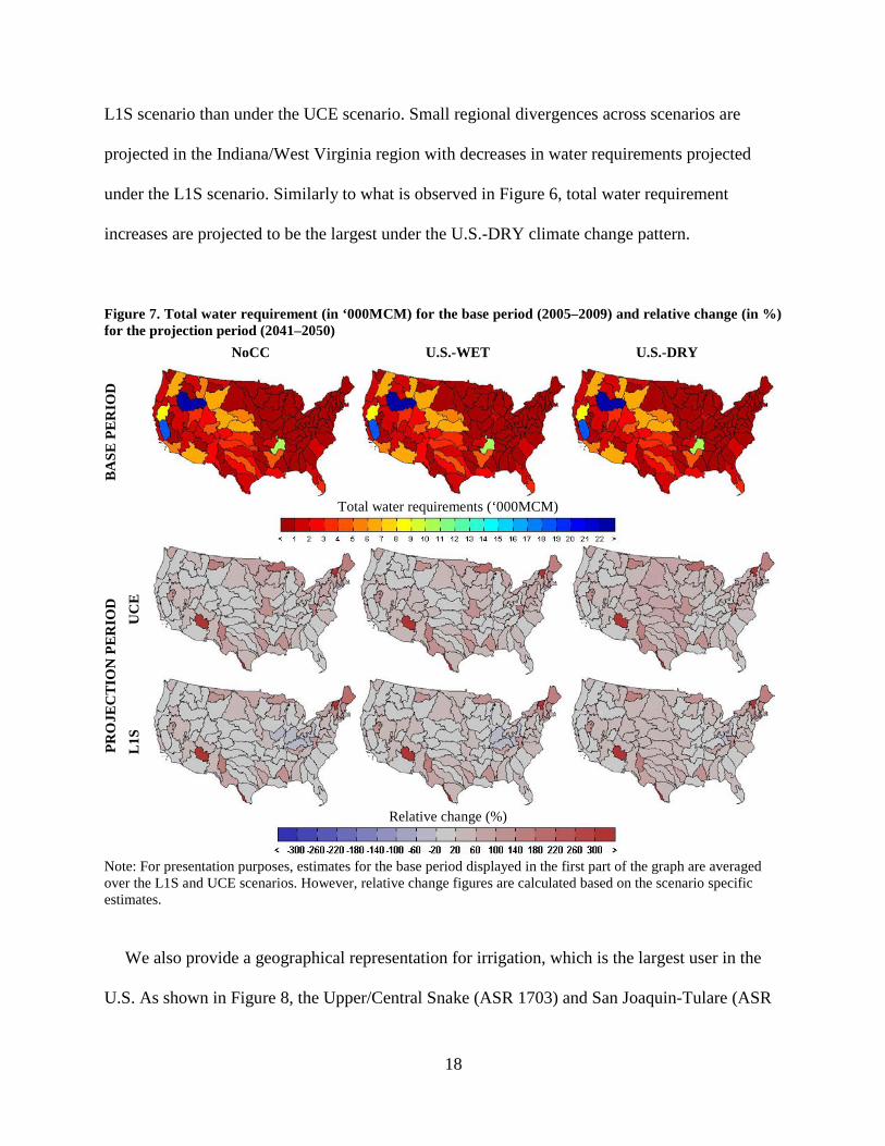
Water requirements at the ASR level are provided in Figure 7 and Figure 8. In these figures,

we first present water requirements in quantitative terms for the base period (2005–2009) and

then show for the projection period (2041–2050) the changes relative to the base period (in %)

under the two scenarios and three climate patterns. Figure 7 shows that the largest water

requirements in the base period originate from the Upper/Central Snake (ASR 1703) and San

Joaquin-Tulare (ASR 1803) basins. In the period 2041 to 2050 total water requirements are

projected to increase by more than 300% in the Little Colorado (ASR 1501), Lower Rio Grande

(ASR 1305) and Richelieu (ASR 106) basins. Increases are generally slightly lower under the

18

L1S scenario than under the UCE scenario. Small regional divergences across scenarios are

projected in the Indiana/West Virginia region with decreases in water requirements projected

under the L1S scenario. Similarly to what is observed in Figure 6, total water requirement

increases are projected to be the largest under the U.S.-DRY climate change pattern.

Figure 7. Total water requirement (in ‘000MCM) for the base period (2005–2009) and relative change (in %) for the projection period (2041–2050)

NoCC U.S.-WET U.S.-DRY

BA

SE P

ER

IOD

Total water requirements (‘000MCM)

PRO

JEC

TIO

N P

ER

IOD

U

CE

L1S

Relative change (%)

Note: For presentation purposes, estimates for the base period displayed in the first part of the graph are averaged over the L1S and UCE scenarios. However, relative change figures are calculated based on the scenario specific estimates.

We also provide a geographical representation for irrigation, which is the largest user in the

U.S. As shown in Figure 8, the Upper/Central Snake (ASR 1703) and San Joaquin-Tulare (ASR

19

1803) basins have the largest irrigation requirements. Very little water is used for irrigation in the

East due to high precipitation and relatively low evaporative demand. Water requirements for

irrigation purposes are expected to increase in the West under both climate change patterns.

Depending on the climate pattern considered, however, irrigation water requirements differ in the

North-Central part of the U.S., with decreases projected under the U.S.-WET climate pattern and

increases under the U.S.-DRY climate pattern. The NoCC climate pattern projects water

requirement increases along the Canadian border. All climate patterns show a decrease in

irrigation water requirements in the Northeast.

Figure 8. Irrigation water requirement (in ‘000MCM) for the base period (2005-2009) and relative change (in %) for the projection period (2041-2050)

NoCC U.S.-WET U.S.-DRY

BA

SE P

ER

IOD

Irrigation water requirements (‘000MCM)

PRO

JEC

TIO

N P

ER

IOD

U

CE

L1S

Relative change (%)

Note: See Note of Figure 7

20

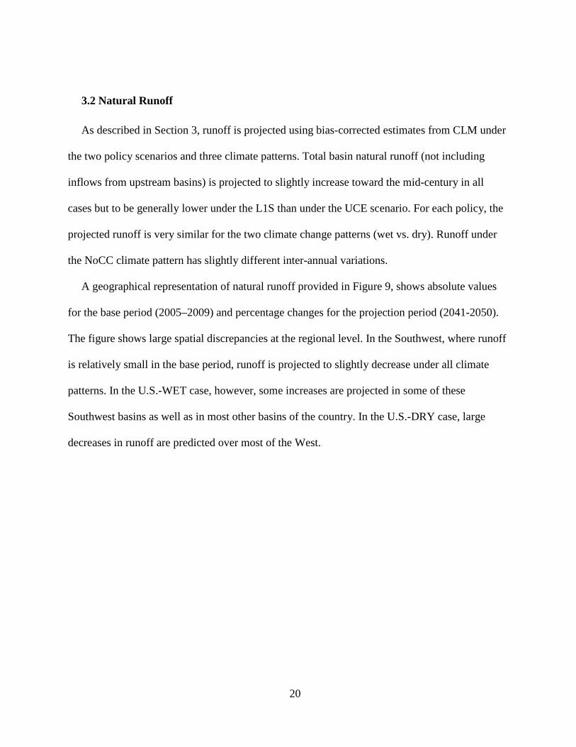
3.2 Natural Runoff

As described in Section 3, runoff is projected using bias-corrected estimates from CLM under

the two policy scenarios and three climate patterns. Total basin natural runoff (not including

inflows from upstream basins) is projected to slightly increase toward the mid-century in all

cases but to be generally lower under the L1S than under the UCE scenario. For each policy, the

projected runoff is very similar for the two climate change patterns (wet vs. dry). Runoff under

the NoCC climate pattern has slightly different inter-annual variations.

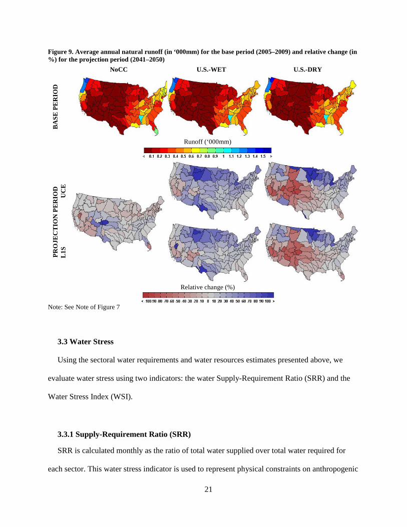
A geographical representation of natural runoff provided in Figure 9, shows absolute values

for the base period (2005–2009) and percentage changes for the projection period (2041-2050).

The figure shows large spatial discrepancies at the regional level. In the Southwest, where runoff

is relatively small in the base period, runoff is projected to slightly decrease under all climate

patterns. In the U.S.-WET case, however, some increases are projected in some of these

Southwest basins as well as in most other basins of the country. In the U.S.-DRY case, large

decreases in runoff are predicted over most of the West.

21

Figure 9. Average annual natural runoff (in ‘000mm) for the base period (2005–2009) and relative change (in %) for the projection period (2041–2050)

NoCC U.S.-WET U.S.-DRY

BA

SE P

ER

IOD

Runoff (‘000mm)

PRO

JEC

TIO

N P

ER

IOD

U

CE

L1S

Relative change (%)

Note: See Note of Figure 7

3.3 Water Stress

Using the sectoral water requirements and water resources estimates presented above, we

evaluate water stress using two indicators: the water Supply-Requirement Ratio (SRR) and the

Water Stress Index (WSI).

3.3.1 Supply-Requirement Ratio (SRR)

SRR is calculated monthly as the ratio of total water supplied over total water required for

each sector. This water stress indicator is used to represent physical constraints on anthropogenic

22

water use. Projections of SRR from 2005 to 2050 are presented in Figure 10 as an annual average

for all ASRs weighted by their sectoral water requirements. The figure shows that water stress is

generally increasing (as the average SRR decreases) under all climate patterns, and especially

under the U.S.-DRY climate pattern. The water stress is slightly smaller under stringent GHG

controls.

Figure 10. Weighted average over all ARS of the mean annual Depletion-Requirements Ratio (SRR) from 2005 to 2050

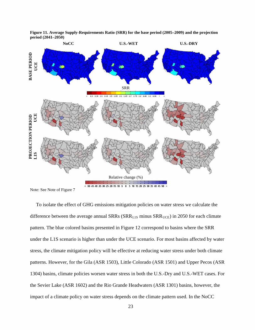
The representation of SRR by ASR provided in Figure 11 indicates that most water

requirements are met in the base period. Water stress is observed in only four basins: Gila (ASR

1503), Sevier Lake (ASR 1602), Rio Grande Headwaters (ASR 1301) and Upper Arkansas (ASR

1102). The SRR is projected to decrease (or remain constant) in all cases, except in the Rio

Grande Headwaters (ASR 1301) basin under the NoCC climate pattern. The largest decreases in

SRR (i.e. increases in water scarcity) are projected in the Little Colorado (ASR 1501) basin

where water requirements are mainly self-supplied. In the U.S.-DRY case, the decrease in SRR

spread further to the North and shows larger reductions overall.

23

Figure 11. Average Supply-Requirements Ratio (SRR) for the base period (2005–2009) and the projection period (2041–2050)

NoCC U.S.-WET U.S.-DRY

BA

SE P

ER

IOD

U

CE

SRR

PRO

JEC

TIO

N P

ER

IOD

U

CE

L1S

Relative change (%)

Note: See Note of Figure 7

To isolate the effect of GHG emissions mitigation policies on water stress we calculate the

difference between the average annual SRRs (SRRL1S minus SRRUCE) in 2050 for each climate

pattern. The blue colored basins presented in Figure 12 correspond to basins where the SRR

under the L1S scenario is higher than under the UCE scenario. For most basins affected by water

stress, the climate mitigation policy will be effective at reducing water stress under both climate

patterns. However, for the Gila (ASR 1503), Little Colorado (ASR 1501) and Upper Pecos (ASR

1304) basins, climate policies worsen water stress in both the U.S.-Dry and U.S.-WET cases. For

the Sevier Lake (ASR 1602) and the Rio Grande Headwaters (ASR 1301) basins, however, the

impact of a climate policy on water stress depends on the climate pattern used. In the NoCC

24

case, where policy scenarios affect water requirements but not water resources, the graph shows

a unanimous beneficial effect of a reduction in water requirements driven by the L1S scenario.

Figure 12. Difference between the average Depletion-Requirements Ratio (SRR) under the L1S and UCE scenarios for each climate pattern in the projection period (2041–2050)

NoCC U.S.-WET U.S.-DRY

SRRL1S - SRRUCE

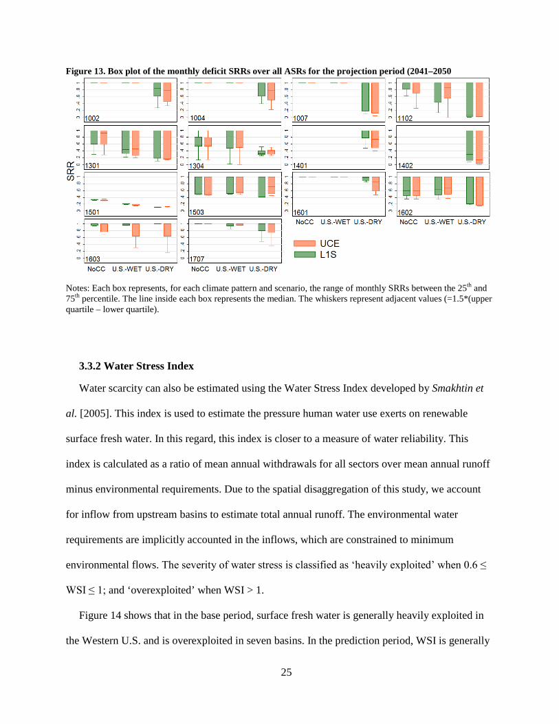
The average number of ASRs affected by monthly water stress (i.e. ASRs where monthly

SRR<1) rises from around 5 (with on average 6 months of water stress per year) in the base

period, to around 7 to 15 (with on average 7 months of water stress per year) in the projection

period. To focus on the effect of water stress within the year, we provide in Figure 13 a series of

box plots of monthly SRRs for the basins significantly affected by water stress in the prediction

period. The figure shows that the spread of the SRRs (i.e. water stress variability) is larger under

the U.S.-DRY case for all basins except the Upper Pecos (ASR 1304) basin. For this basin, the

plot shows that the water stress is consistently more important under the U.S.-DRY case than

under the U.S.-WET case. The boxes for the L1S scenario are generally smaller and closer to one

than those for the UCE scenario, which shows that the climate policy is effective at reducing

water stress severity and variability.

25

Figure 13. Box plot of the monthly deficit SRRs over all ASRs for the projection period (2041–2050

Notes: Each box represents, for each climate pattern and scenario, the range of monthly SRRs between the 25th and 75th percentile. The line inside each box represents the median. The whiskers represent adjacent values (=1.5*(upper quartile – lower quartile).

3.3.2 Water Stress Index

Water scarcity can also be estimated using the Water Stress Index developed by Smakhtin et

al. [2005]. This index is used to estimate the pressure human water use exerts on renewable

surface fresh water. In this regard, this index is closer to a measure of water reliability. This

index is calculated as a ratio of mean annual withdrawals for all sectors over mean annual runoff

minus environmental requirements. Due to the spatial disaggregation of this study, we account

for inflow from upstream basins to estimate total annual runoff. The environmental water

requirements are implicitly accounted in the inflows, which are constrained to minimum

environmental flows. The severity of water stress is classified as ‘heavily exploited’ when 0.6 ≤

WSI ≤ 1; and ‘overexploited’ when WSI > 1.

Figure 14 shows that in the base period, surface fresh water is generally heavily exploited in

the Western U.S. and is overexploited in seven basins. In the prediction period, WSI is generally

26

increasing in the Central and Western U.S. under the U.S.-DRY climate pattern and decreasing

in the Northeast. In the U.S.-WET case, the WSI is projected to decrease generally, except on the

coasts. The WSI is projected to increase more uniformly under the NoCC climate pattern.

This index shows that although most basins will not be affected by unmet water requirements

as shown by the SRR ratio, a large number of basins in the West will experience increasing

pressure on water resources. This will be especially the case under the U.S.-DRY climate pattern,

where over exploited basins are more prone to water shortages.

Figure 14. Average Water Stress Index (WSI) for the base period (2005–2009) and the projection period (2041–2050)

NoCC U.S.-WET U.S.-DRY

BA

SE P

ER

IOD

U

CE

WSI

PRO

JEC

TIO

N P

ER

IOD

U

CE

L1S

Relative change (%)

Note: See Note of Figure 7

27

4 Conclusions

This paper presents WRS-US, a model of U.S. water resource systems. For this exercise, we

downscale the IGSM-WRS model to the 99 ASR level for the continental U.S. We also produce

new estimates of water resources and water requirements for five sectors. WRS-US is used to

allocate these water resources among the different sectors to minimize water stress, which

measures the degree to which water requirements that cannot be met. As an illustration, the

model is used to project water stress through 2050 under two climate policies.

We estimate that, with or without climate change, average annual water stress is predicted to

increase most in the Southwest. This increase is mostly attributable to increases in water

requirements. The study reveals that the choice of climate pattern considered for projections

greatly influences the outcome of the model. On average, larger water stresses are projected

under the U.S.-DRY climate pattern, than under the U.S.-WET pattern. The impact of a

constrained GHG emission policy (L1S scenario) will generally lessen the increase of mean

annual water stress, especially in the U.S.-DRY case. However, in some basins water stress will

be lower under an unconstrained emission policy (UCE scenario) than under a climate policy. A

more detailed analysis of water stress at the monthly level reveals that the extent and intensity of

monthly water stress is less under the L1S scenario than under the UCE scenario in most basins.

The WSI index, representing the reliability of water resources, shows that, although most basins

will not be affected by unmet water requirements in the future (as shown by the SRR ratio), a

large number of basins in the West will see increased pressure on water resources, especially

under the U.S.-DRY climate pattern.

In developing an integrated model of changes in water supply, climate change, and water use,

some simplifications are necessary. The most important of these simulations is the assumption

that irrigated areas remain unchanged in the future. In principle, we may see adjustments in areas

28

that are regularly short of water for irrigation because maintenance of irrigation infrastructure

may become uneconomic. On the other hand, irrigation may expand in areas where water

supplies are ample but crop yields are reduced because of increased droughts. We identify those

areas where water stress increases, and where it therefore may become uneconomic to maintain

irrigation infrastructure at its current level. Whether losses of food production in these regions

would be replaced through dryland or irrigated cropland elsewhere in the U.S. or abroad requires

further investigation and modeling. We also assume that current rates of groundwater withdrawal

are sustainable. If they are not, either because withdrawal currently exceeds recharge or climate

changes in such a way as to reduce recharge, then irrigation dependent on groundwater may

cease in these areas with possible increased pressure on surface water flows.

Notwithstanding these simplifications, WRS-US is an important tool for water resource

planning and management. It has the substantial advantages over other water models to be part of

the IGSM which allows integrated assessments of water resources and uses in the context of

climate and economic effects. The current estimation of climate change also allows the

estimation of climate change uncertainty on water resources and ultimately on water stress. The

framework will also support the development of feedbacks to assess the implications of water

stress on the economy. This model also represents a significant improvement compared to global

water models. First, by focusing on the U.S. we take advantage of water-use data detailed at the

county level to estimate and project detailed sectoral water requirements. The spatial

disaggregation allows the detection of local water issues, such as the water deficit in the West.

Future applications could focus on the impact of such water stress on economic activities, such

as food production or naval transportation. This downscaled model also lays the foundations for

29

further investigation of water allocation strategies, which are not possible at wide river basin

delineations.

Acknowledgments

The Joint Program on the Science and Policy of Global Change is funded by the U.S.

Department of Energy, Office of Science under grants DE-FG02-94ER61937, DE-FG02-

93ER61677, DEFG02-08ER64597, and DE-FG02-06ER64320; the U.S. Environmental

Protection Agency under grants XA-83344601-0, XA-83240101, XA-83042801-0, PI-83412601-

0, RD-83096001, and RD-83427901-0; the U.S. National Science Foundation under grants SES-

0825915, EFRI-0835414, ATM-0120468, BCS-0410344, ATM-0329759, and DMS-0426845;

the U.S. National Aeronautics and Space Administration under grants NNX07AI49G,

NNX08AY59A, NNX06AC30A, NNX09AK26G, NNX08AL73G, NNX09AI26G,

NNG04GJ80G, NNG04GP30G, and NNA06CN09A; the U.S. National Oceanic and

Atmospheric Administration under grants DG1330-05-CN-1308, NA070AR4310050, and

NA16GP2290; the U.S. Federal Aviation Administration under grant 06-C-NE-MIT; the Electric

Power Research Institute under grant EPP32616/C15124; and a consortium of 40 industrial and

foundation sponsors (for the complete list see http://globalchange.mit.edu/sponsors/current.html)

References

Blanc, E., K. Strzepek, C. A. Schlosser, H. D. Jacoby, A. Gueneau, C. Fant, S. Rausch, and J. M.

Reilly (2013), Analysis of u.S. Water resources under climate changeRep.

Clarke, L., J. Edmonds, H. Jacoby, H. Pitcher, J. Reilly, and R. Richels (2007), Scenarios of

greenhouse gas emissions and atmospheric concentrations, sub-report 2.1a of synthesis and

assessment product 2.1 Rep., 106 pp, U.S. Climate Change Science Program and the

Subcommittee on Global Change Research, Department of Energy, Office of Biological and

Environmental Research, Washington, DC., USA.

Collins, W. D., et al. (2006), The community climate system model version 3 (CCSM3), Journal

of Climate, 19, 2122-2143.

Connell-Buck, C. R., J. Medellín-Azuara, J. R. Lund, and K. Madani (2011), Adapting

california’s water system to warm vs. Dry climates, Climatic Change, 109(Suppl 1), 133-149.

30

Delworth, T. L., and Coauthors (2006), GFDL's cm2 global coupled climate models. Part i:

Formulation and simulation characteristics, Journal of Climate, 19, 643-674.

Fant, C., K. Strzepek, A. Gueneau, S. Awadalla, E. Blanc, W. Farmer, and C. A. Schlosser

(2011), Clicrop: A crop water-stress and irrigation demand model for an integrated global

assessment modeling approachRep.

Forest, C. E., P. H. Stone, and A. P. Sokolov (2008), Constraining climate model parameters

from observed 20th century changes, Tellus, 60(5), 911-920.

Hirji, R., and R. Davis (2009), Environmental flows in water resources policies, plans, and

projects: Case studiesRep., The World Bank Environment Department.

Lawrence, D., et al. (2011), Parameterization, improvements and functional and structural

advances in version 4 of the community land model, Journal of Advances in Modeling Earth

Systems, 3(1).

Meehl, G. A., C. Covey, T. Delworth, M. Latif, B. McAvaney, J. F. B. Mitchell, R. J. Stouffer,

and K. E. Taylor (2007), The WCRP CMIP3 multi-model dataset: A new era in climate

change research, Bulletin of the American Meteorological Society, 88, 1383-1394.

NCAR (2012), Community land model Rep., National Center for Atmospheric Research.

Paltsev, S., J. M. Reilly, H. D. Jacoby, R. S. Eckaus, J. McFarland, M. Sarofim, M. Asadoorian,

and M. Babiker (2005), The MIT emissions prediction and policy analysis (EPPA) model:

Version 4Rep.

Postel, S. (2000), Entering an era of water scarcity: The challenges ahead, Ecological

applications, 10, 941-948.

Rausch, S., and M. Mowers (2012), Distributional and efficiency impacts of clean and renewable

energy standards for electricityRep.

Rausch, S., G. E. Metcalf, J. M. Reilly, and S. Paltsev (2010), Distributional impacts of a u.S.

Greenhouse gas policy: A general equilibrium analysis of carbon pricing, in U.S. Energy tax

policy, edited.

Rosegrant, M. W., C. Ringler, S. Msangi, T. B. Sulser, T. Zhu, and S. A. Cline (2008),

International model for policy analysis of agricultural commodities and trade (impact): Model

descriptionRep., International Food Policy Research Institute, Washington, D.C.

Scanlon, B., R. Healy, and P. Cook (2002), Choosing appropriate techniques for quantifying

groundwater recharge, Hydrogeology Journal, 10(1), 18-39.

31

Schlosser, C. A., X. Gao, K. Strzepek, A. Sokolov, C. E. Forest, S. Awadalla, and W. Farmer

(2012), Quantifying the likelihood of regional climate change: A hybridized approach,

Journal of Climate.

Short, W., N. Blair, P. Sullivan, and T. Mai (2009), Reeds model documentation: Base case data

and model descriptionRep., National Renewable Energy Laboratory.

Smakhtin, V., C. Revenga, and P. Döll (2004), A pilot global assessment of environmental water

requirements and scarcity, Water International, 29, 307-317.

Smakhtin, V., C. Revanga, and P. Doll (2005), Taking into account environmental water

requirements in globalscale water resources assessmentsRep.

Sokolov, A. P., et al. (2005), The MIT integrated global system model (IGSM) version 2: Model

description and baseline evaluationRep., MIT Joint Program on the Science and Policy of

Global Change.

Strzepek, K., J. Baker, W. Farmer, and C. A. Schlosser (2012a), Modeling water withdrawal and

consumption for electricity generation in the united statesRep.

Strzepek, K., C. A. Schlosser, A. Gueneau, X. Gao, É. Blanc, C. Fant, B. Rasheed, and H. D.

Jacoby (2012b), Modeling water resource systems under climate change: IGSM-WRSRep.

Templin, W. E., R. A. Herbert, C. B. Stainaker, M. Horn, and W. B. Solley (1997), Chapter 11 -

water use, in National handbook of recommended methods for water data acquisition, edited,

US Geological Survey.

U.S. Bureau of Reclamation (2009), Colorado river accounting and water use reportRep., U.S.

Bureau of Reclamation.

U.S. Census Bureau (2000), U.S. Population projections: State interim population projections by

age and sex: 2004-2030Rep.

UN (2012), The millennium development goals report 2012Rep.

USDA (2003), 2003 farm and ranch irrigation surveyRep., United States Department of

Agriculture.

USGS (2011), Water use in the united states, http://water.usgs.gov/watuse/data/.

USGS (2012), General facts and concepts about ground

water http://pubs.usgs.gov/circ/circ1186/html/gen_facts.html.

USWRC (1978), The nation's water resources 1975-2000, U.S. Government Printing Office,

Washington, D.C.

32

van der Gun, J. (2012), Groundwater and global change: Trends, opportunities and

challengesRep., UNESCO, Paris.

Zetland, D. (2011), Colorado river aqueduc, in Encyclopedia of water politics and policy in the

united states, edited by B. J. Danver SL, CQ Press/SAGE, Washington, DC.